Parameter Estimation Guidelines for Risk-Based Corrective Action ...

Groundwater Services, Inc. 

Parameter Estimation Guidelines for 

Risk-Based Corrective Action (RBCA) Modeling 

John A. Connor, P.E. Charles J. Newell, Ph.D., P.E. Mark W. Malander, CPG 

Groundwater Services, Inc. Groundwater Services, Inc. Mobil Oil Corporation 

Abstract 

For use in risk-based corrective action (RBCA) analyses, simple analytical fate-and-transport 

models can provide a cost-effective means of estimating exposure concentrations and developing 

risk-based soil and groundwater remediation standards. Under ASTM E-1739 "Standard Guide for 

Risk-Based Corrective Action Applied at Petroleum Release Sites," such models are recommended 

as a conservative first step under Tiers 1 and 2 of the site evaluation process, prior to use of more 

complex numerical modeling methods under Tier 3. However, the reliability of an analytical model 

as a conservative predictor of chronic exposure levels depends upon proper characterization of key 

physical and chemical parameters. 

This paper reviews a system of analytical fate-and-transport models compiled expressly for use 

with the ASTM RBCA Standard and provides practical guidelines for measurement and/or 

estimation of key input parameters for each model. Contaminant transport pathways addressed in 

this paper include soil-to-air volatilization, soil-to-groundwater leaching, lateral air transport, and 

lateral groundwater transport. Parameter selection guidelines discussed in this paper relate 

specifically to the analytical expressions listed in Appendix X.2 of ASTM E-1739. However, these 

guidelines are generally applicable to a broad range of soil, air, and groundwater transport models. 

RBCA Spreadsheet System 

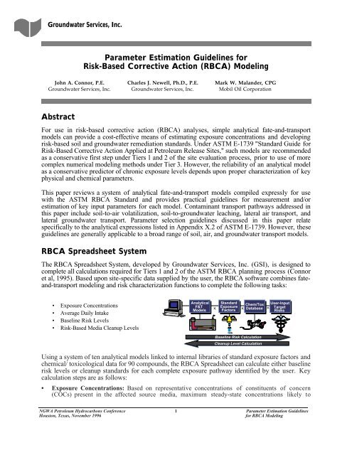
The RBCA Spreadsheet System, developed by Groundwater Services, Inc. (GSI), is designed to 

complete all calculations required for Tiers 1 and 2 of the ASTM RBCA planning process (Connor 

et al, 1995). Based upon site-specific data supplied by the user, the RBCA software combines fateand-transport 

modeling and risk characterization functions to complete the following tasks: 

• Exposure Concentrations 

• Average Daily Intake 

• Baseline Risk Levels 

• Risk-Based Media Cleanup Levels 

Analytical 

F&T 

Models 

Standard 

Chem/Tox 

x Exposure x 

= 

Factors 

Database 

, 

, 

Baseline Risk Calculation 

Cleanup Level Calculation 

User-Input 

Target 

Risks 

Using a system of ten analytical models linked to internal libraries of standard exposure factors and 

chemical/ toxicological data for 90 compounds, the RBCA Spreadsheet can calculate either baseline 

risk levels or cleanup standards for each complete exposure pathway identified by the user. Key 

calculation steps are as follows: 

• Exposure Concentrations: Based on representative concentrations of constituents of concern 

(COCs) present in the affected source media, maximum steady-state concentrations likely to 

NGWA Petroleum Hydrocarbons Conference 1 Parameter Estimation Guidelines 

Houston, Texas, November 1996 

for RBCA Modeling


occur at the point of exposure (POE) are calculated using the steady-state analytical fate-andtransport 

models identified in Appendix X.2 of ASTM E-1739. To perform these calculations, 

the system evaluates cross-media partitioning (e.g., volatilization from soil to air) and lateral 

transport from the source to the POE (e.g., contaminant transport via air or groundwater flow). 

The source media and optional exposure pathways included in the software as as follows: 

SOURCE MEDIA 

Surface Soils 

Subsurface Soils 

Groundwater 

EXPOSURE PATHWAYS 

• Inhalation of Volatiles and Particulates 

• Dermal Contact with Soil 

• Ingestion of Soil and Dust 

• Leaching to Groundwater/Ingestion 

• Inhalation of Volatiles 

• Leaching to Groundwater/Ingestion 

• Ingestion of Potable Water 

• Inhalation of Volatiles 

• Average Daily Intake: Based upon the exposure factors selected by the user, the average daily 

chemical intake for each receptor along each selected pathway is calculated in accordance with 

EPA guidelines (see Connor et al, 1995). These values are used in baseline risk calculations for 

each complete pathway. 

• Baseline Risk Characterization: Human health risks associated with exposure to COCs are 

calculated by the spreadsheet on the basis of average daily intake rates and the corresponding 

toxicological parameters for carcinogenic and non-carcinogenic effects. For each complete 

pathway, the system output provides both individual and additive constituent results for 

carcinogens and non-carcinogens. 

• Media Cleanup Values: The RBCA Spreadsheet System has the ability to i) compare site data to 

Tier 1 Risk-Based Screening Levels (RBSLs), computed using default parameter values as listed in 

ASTM E-1739, or ii) calculate Tier 2 Site-Specific Target Levels (SSTLs) based on user-supplied 

site characterization information. For each source medium (i.e., affected soil and groundwater), 

the software reports target concentrations for all complete pathways and identifies the applicable 

(i.e., minimum) value for source remediation. 

Fate and Transport Modeling Methods 

The RBCA Spreadsheet System contains a series of fate and transport models for predicting COC 

concentrations at the point of exposure (POE) for each of the optional exposure pathways listed 

above. Under Tier 2 of the RBCA process, relatively simple analytical models are to be employed 

for this calculation, representing a minor incremental effort relative to Tier 1. The spreadsheet 

modeling system is consistent with Appendix X.2 of ASTM E-1739, although selected algorithms 

and default parameters have been updated to reflect advances in evaluation methods. 

The idealized schematic shown on Figure 1 illustrates the steps for predicting transport of 

contaminants from the source zone to the POE for air and groundwater exposure pathways. Each 

element in Figure 1 represents a step-specific attenuation factor, corresponding to either a crossmedia 

transfer factor (CM) or a lateral transport factor (LT). The effective natural attenuation factor 

(NAF) for each COC on each pathway is then calculated as the arithmetic product of the various 

attenuation factors occurring along the flow path from source to receptor. These steady-state NAF 

values are then used for calculation of baseline risks and back-calculation of Site-Specific Target 

Levels (SSTLs), as discussed above. Please note that fate and transport modeling is not required 

for exposure via direct contact with the source medium, such as soil ingestion or dermal contact, 





where the source and exposure concentrations are equal (i.e., NAF = 1). Analytical models used 

for conservative estimation of each transport factor per ASTM E-1739 are described below. 

INDIRECT 

EXPOSURE 

PATHWAY 

SOURCE 

MEDIUM 

CROSS-MEDIA 

TRANSFER FACTORS 

LATERAL 

TRANSPORT 

FACTORS 

EXPOSURE 

MEDIUM 

TOTAL 

PATHWAY 

NAF 

Air Exposure Pathways 

• Surface Soil: 

Volatilization 

and dust 

releases to 

ambient air 

Affected 

Surface 

Soil 

Equation CM-1 

Surface 


Factor (VF ss) 

Equation CM-2 

Particulate 

Emission 

Factor (PEF) 

Equation LT-2 

Lateral Air 

Dispersion 

Factor (ADF) 

Ambient 

Air 

at POE 

ADF 

VF ss+ PEF 

• Subsurface 

Soil: 


to ambient air 

Affected 

Subsurface 

Soils 

Equation CM-3 

Subsurface 


Factor (VF samb) 

Equation LT-2 

Lateral Air 

Dispersion 

Factor (ADF) 

Ambient 

Air 

at POE 

ADF 

VF samb 

• Subsurface 

Soil: 


to enclosed 

space 

Affected 

Subsurface 

Soils 

Equation CM-4 

Soil to 

Enclosed Space 


Factor (VF sesp ) 

Indoor 

Air 

at POE 

1 

VF sesp 

• Groundwater: 


to ambient air 

Affected 

Groundwater 

Equation CM-5 

Groundwater 


Factor (VF wamb) 

Equation LT-2 

Lateral Air 

Dispersion 

Factor (ADF) 

Ambient 

Air 

at POE 

ADF 

VF wamb 

• Groundwater: 


to enclosed 

space 

Affected 

Groundwater 

Equation CM-6 

Groundwater to 

Enclosed Space 


Factor (VF wesp) 

Indoor 

Air 

at POE 

1 

VF wesp 

Groundwater Exposure Pathways 

• Soil: Leaching 

to groundwater/ 

ingestion and 

dermal contact 

Affected 

Soils 

Equation CM-7 

Soil to 

Leachate 

Partition 

Factor (K sw) 

Equation CM-8 

Leachate- 

Groundwater 

Dilution 

Factor (LDF) 

Equation LT-1 

Lateral Groundwater 

Dilution-Attenuation 

Factor (DAF) 

Groundwater 

at POE 

LDF X DAF 

K sw 

• Dissolved 

or Free-Phase 

Groundwater 

Plume: 

Ingestion and 

dermal contact 

Affected 

Groundwater 

Equation LT-1 

Lateral Groundwater 

Dilution-Attenuation 

Factor (DAF) 

Groundwater 

at POE 

DAF 

FIGURE 1. NAF CALCULATION SCHEMATIC FOR EXPOSURE PATHWAYS IN RBCA SPREADSHEET SYSTEM 

CROSS-MEDIA TRANSFER FACTORS 

Exposure pathways involving transport of COCs from one medium to another (e.g., soil-to-air, 

soil-to-groundwater) require estimation of the corresponding cross-media transfer factor. Various 

analytical expressions are available for estimating soil-to-air volatilization factors as a function of 

site soil characteristics and the physical/chemical properties of volatile organic COCs. Leaching 

factors for organic and inorganic constituent releases from soil to groundwater can similarly be 

estimated as a function of COC characteristics, soil conditions, and annual rainfall infiltration. 

Cross-media transfer equations incorporated in the RBCA Spreadsheet System are presented in 

Figure 2. Detailed discussion of each of these cross-media factors is provided in the Tier 2 RBCA 

Guidance Document (Connor et al, 1995). 





Equation CM-1: Surface Soil Volatilization Factor (VFss) 

Uair 

breathing zone 

d affected surficial soils 

W 

δ air 

diffusing 

vapors 

CM-1a: 

VF 

ss 

( ) 

3 

⎡ 

eff 

mg / m − air ⎤ 2W 

s 

Ds 

H 

⎢ 

⎥ 

⎣⎢ 

( mg / kg − soil) 

⎦⎥ = ρ 

Uairδair 

πτ θ + k ρ + Hθ 

or CM-1b: 

VF 

whichever is less 

Equation CM-2: Soil Particulate Emission Factor (PEF) 

ss 

( ) 

3 

⎡ mg / m − air 

⎢ 

⎣⎢ 

mg / kg − soil 

( ) 

( ) × 

ws s s as 

⎤ Wρsd 

⎥ = × 10 

⎦⎥ 

Uairδairτ 

3 

10 

3 

Uair 

d 

P e 


affected surficial soils 

δ air 

diffusing 

vapors 

( ) 

3 

⎡ mg / m − air 

PEF⎢ 

⎣⎢ 

mg / kg − soil 

( ) 

⎤ PW 

e 

⎥ = × 10 

⎦⎥ 

Uairδ 

air 

3 

W 

Equation CM-3: Subsurface Soil Volatilization Factor (VFsamb) 

L s 

U air 

breathing zone δair 

vadose zone 

d i f f u s i n g v a p o r s 

affected subsurface soils 

W 

CM-3a: 

⎡ 3 

( mg / m − air) 

⎤ 

H 

VF ⎢ 

⎥ 

s 

samb 

⎢( mg / kg − soil) 

⎥ = ρ 

⎡ 

⎣ 

⎦ θws + ksρs + Hθas 

⎢1 

⎣⎢ 

or CM-3b: 


[ ] + 

( ) 

⎡ 3 

mg / m − air 

VF ⎢ 

samb 

⎢ mg / kg − soil 

⎣ 

( ) 

3 

x10 

Uairδair L ⎤ 

s 

Ds eff ⎥ 

W ⎦⎥ 

⎤ 

⎥ W sds 

3 

10 

⎥ = ρ 

Uairδairτ x 

⎦ 

Equation CM-4: Subsurface Soil to Enclosed Space Volatilization Factor (VFsesp) 

ER: air 

exchange 

rate 

L s 

enclosed-space 

foundation cracks 

,,,,,,,,,,,,,, 

d i f f u s i n g 

affected subsurface soils 

W 

v a p o r s 

L 

b 

: Vol. / Infil. Area Ratio 

L crack : Foundation 

Thickness 

vadose zone 

CM-4a: 

Hρ 

⎡ 

s Ds eff / L ⎤ 

s 

⎡ 3 

( mg / m − air) 

⎤ 

⎢ ⎥ 

ws ks s H as ER LB 

VF ⎢ 

⎥ 

[ 3 

sesp 

10 

⎢( mg / kg − soil) 

⎥ = θ + ρ + θ ] ⎣⎢ 

⎦⎥ 

x 

⎣ 

⎦ Ds eff / Ls 

Ds eff / L 

1 + ⎡ s 

ER L eff 

⎣ ⎢ ⎤ 

⎡ 

⎤ 

⎥ 

⎢ B ⎦⎥ + ⎢ 

⎥ 

( Dcrack 

/ L 

⎣⎢ 

crack ) η 

⎦⎥ 

or CM-4b: 


( ) 

⎡ 3 

mg / m − air 

VF ⎢ 

sesp 

⎢ mg / kg − soil 

⎣ 

( ) 

⎤ 

⎥ sds 

3 

10 

⎥ = ρ LBERτ x 

⎦ 

FIGURE 2. CROSS-MEDIA PARTITIONING EQUATIONS IN THE RBCA SPREADSHEET SYSTEM 

Continued 





Continued 

Equation CM-5: Groundwater Volatilization Factor (VFwamb) 

Uair 


δ air 

L gw 

h v d i f f u s i n g v a p o r s 

h 

c 

dissolved plume 

groundwater 

vadose zone 

capillary zone 

( ) 

⎡ 3 

mg / m − air ⎤ 

VF ⎢ 

⎥ 

3 

wamb 

10 

⎢ ( mg/L − H2O) 

⎥ = Η 

Uair air L 

⎣ 

⎦ 1 + ⎡ x 

GW 

eff 

⎣ ⎢ δ ⎤ 

⎥ 

⎢ WDws 

⎦⎥ 

W 

Equation CM-6: Groundwater to Enclosed Space Volatilization Factor (VFwesp) 

L 

b 

: Vol. / Infil. Area Ratio 

L crack : Foundation 

ER: air 

Thickness 

exchange 

enclosed-space 

rate 

foundation cracks 

,,,,,,,,,,,,,, 

,,,,,,,,,,,,,, 

vadose zone 

h v 

L gw 

d i f f u s i n g v a p o r s 

h c 


capillary zone 

⎡ 

H D eff 

ws / L ⎤ 

GW 

⎡ 3 

( mg / m − air) 

⎤ 

⎢ ⎥ 

ER LB 

VF ⎢ 

⎥ 

3 

wesp 

10 

⎢( mg / L − H2O) 

⎥ = 

⎣⎢ 

⎦⎥ 

x 

eff 

eff 

⎣ 

⎦ Dws 

/ LGW 

Dws 

/ LGW 

1 + ⎡ ⎤ 

⎡ 

⎤ 

⎢ ⎥ 

ER L 

eff 

⎣⎢ 

B ⎦⎥ + ⎢ 

⎥ 

( Dcrack 

/ L 

⎣⎢ 

crack ) η 

⎦⎥ 

groundwater 

W 

Equation CM-7: Soil Leachate Partition Factor(Ksw) 

Equation CM-8: Leachate-Groundwater Dilution Factor (LDF) 

I: Infiltration Rate 

affected soils 

vadose zone 

( ) 

⎡ mg / L − H2O 

⎤ ρ 

K 

s 

sw ⎢ 

⎥ = 

⎣ ( mg/kg − soil) 

⎦ θws + ksρs + Hθas 

V gw 

leachate 


groundwater 

W 

δgw 

mixing 

zone 

Vgwδgw 

LDF[ dimensionless]= 1 + 

IW 


Continued 





Continued 

Definitions for Cross-Media Transfer Equations 

D s 

eff 

eff 

D ws 

Effective diffusivity in vadose zone soils: 

eff ⎡ cm 2 ⎤ 

D s ⎢ ⎥ 

⎣⎢ 

s 

⎦⎥ = θ Dair as 

3.33 ⎡ 

+ Dwat ⎤ 

2 ⎢ ⎥ 

θ T ⎣⎢ 

H 

⎦⎥ 

⎡ 3.33 

θ ws 

⎤ 

⎢ 2 ⎥ 

⎣⎢ 

θ T ⎦⎥ 

Effective diffusivity above the water table: 

D 

eff 

ws 

⎡ 

⎢ 

cm ⎣ s 

2 

⎤ 

⎥ = hcap 

+ h 

⎦ 

⎡ h 

⎢ 

⎣⎢ 

D 

( 

cap 

v ) eff 

+ 

cap 

h 

D 

v 

eff 

s 

d Lower depth of surficial soil zone (cm) 

d s Thickness of affected subsurface soils 

D air Diffusion coefficient in air (cm 2 /s) 

D wat Diffusion coefficient in water (cm 2 /s) 

ER Enclosed-space air exchange rate (l/s) 

f oc Fraction of organic carbon in soil (g-C/g-soil) 

H Henry’s law constant (cm 3 -H 2 O)/(cm 3 -air) 

h cap Thickness of capillary fringe (cm) 

h v Thickness of vadose zone (cm) 

I Infiltration rate of water through soil (cm/year) 

k oc Carbon-water sorption coefficient (g-H 2 O/g-C) 

k s Soil-water sorption coefficient (g-H 2 O/g-soil) 

L B Enclosed space volume/infiltration area ratio (cm) 

L crack Enclosed space foundation or wall thickness (cm) 

L GW Depth to groundwater = h cap + h v (cm) 

L s Depth to subsurface soil sources (cm) 

P e Particulate emission rate (g/cm 2 -s) 

U air Wind speed above ground surface in ambient mixing 

zone (cm/s) 

V gw Groundwater Darcy velocity (cm/s) 

⎤ 

⎥ 

⎦⎥ 

−1 

eff 

D crack 

eff 

D cap 

W 

δ air 

δ gw 

η 

Effective diffusivity through foundation cracks: 

eff ⎡ cm 2 ⎤ 

D crack ⎢ ⎥ 

⎣⎢ 

s 

⎦⎥ = θ 3.33 ⎡ 

Dair acrack 

+ Dwat ⎤ ⎡ 

2 ⎢ ⎥ ⎢ 

θ T ⎣⎢ 

H 

⎦⎥ 

⎣⎢ 

Effective diffusivity in the capillary zone: 

eff ⎡ cm 2 ⎤ 

D cap ⎢ ⎥ 

⎣⎢ 

s 

⎦⎥ = θ 3.33 

Dair acap ⎡ 

+ Dwat ⎤ 

2 ⎢ ⎥ 

θ T ⎣⎢ 

H 

⎦⎥ 

3.33 

θ wcrack 

2 

θ T 

⎡ 3.33 

θ wcap 

⎤ 

⎢ ⎥ 

2 

⎢ 

⎣ 

θ T ⎥ 

⎦ 

Width of source area parallel to wind, or groundwater flow 

direction (cm) 

Ambient air mixing zone height (cm) 

Groundwater mixing zone thickness (cm) 

Areal fraction of cracks in foundations/walls 

(cm 2 -cracks/cm 2 -total area) 

θacap Volumetric air content in capillary fringe soils 

(cm 3 -air/cm 3 -soil) 

θ acrack Volumetric air content in foundation/wall cracks 

(cm 3 -air/cm 3 total volume) 

θ as 

Volumetric air content in vadose zone soils 

(cm 3 -air/cm 3 -soil) 

θ T Total soil porosity (cm 3 -pore-space/ cm 3 -soil) 

θwcap Volumetric water content in capillary fringe soils 

(cm 3 -H 2 O/cm 3 -soil) 

θ wcrack Volumetric water content in foundation/wall cracks 

(cm 3- H 2 O)/cm 3 total volume) 

θ ws Volumetric water content in vadose zone soils 

(cm 3 -H 2 O/cm 3 -soil) 

ρ s Soil bulk density (g-soil/cm 3 -soil) 

τ Averaging time for vapor flux (s) 

⎤ 

⎥ 

⎦⎥ 


LATERAL TRANSPORT FACTORS 

During lateral transport within air or groundwater, COC concentrations in the flow stream will be 

diminished due to mixing and attenuation effects (see Figure 1). Site-specific attenuation factors 

characterizing COC mass dilution or loss during lateral transport can be estimated using the air 

dispersion and groundwater transport models provided in the RBCA Spreadsheet System. Equations for 

the steady-state analytical transport models incorporated in the RBCA spreadsheet are shown on 

Figure 3. Equations LT-1 and LT-2 correspond to the Domenico 3-D groundwater solute transport model 

and the standard gaussian air dispersion model, respectively. The user must provide information 

regarding COC properties and transport parameters (flow velocities, dispersion coefficients, 

retardation factors, decay factors, etc.), as required for the selected contaminant transport model. 

Procedures for definition of the contaminant source term for the groundwater solute model (Equation LT- 

1) are illustrated on Figure 4. Key assumptions of these lateral transport models are detailed in the 

Tier 2 RBCA Guidance Manual (Connor et al, 1995). 





Equation LT- 1: Lateral Groundwater Dilution Attenuation Factor 

Groundwater 

Flow Direction 

Sd 

α x 

α z 

α y 

⎡ 

⎛ 

S 

⎞ 

Cx ( ) i 

= ( C si + BC w 

i )erf 

⎜ 4 α y x ⎟ erf 

⎛ S d 

⎞ 

⎢ 

⎢ 

⎜ ⎟ 

⎝ ⎠ ⎝ 4 α z x ⎠ 

⎣ 

Dispersivity 

C 

where: BCi 

= BCT 

x si and BCT 

= Σ 

∑ Csi 

LT-1a: Solute Transport with First-Order Decay: 

Cx ( ) ⎛ 

i x ⎡ 4λiα 

xR 

⎤⎞ 

⎛ 

i S ⎞ 

= exp − + erf w 

⎜ ⎢1 1 ⎥⎟ 

S w 

Csi ⎝ 2 α x ⎣⎢ 

⎦⎥ 

⎠ 

⎜ ⎟ 

⎝ y ⎠ 

X 

where: 

K⋅ 

i 

ν = 

θe 

LT-1b: Solute Transport with Biodegradation by Electron- 

Acceptor Superposition Method: 

Csource C (x) 

Plume Source 

Predicted 

Plume 

Migration 

Equation LT-2: Lateral Air Dispersion Factor 

x erf 

⎛ S ⎞ 

d 

ν 4 α 

⎜ 

⎝ 4 αzx 

⎟ 

⎠ 

⎤ 

⎥ 

⎥ − BC i 

⎦ 

Cea ( ) n 

UFn 

[Note: For Equations LT-1a and LT-1b, NAF = Csi/C(x)i] 

Wind 

direction 

Uair 

C s (point source) 

y 

δair 

L 

Ground surface 

Source zone 

x 

box model 

(Equations CM-1, CM-2, CM-3) 

C x 

z 

( ) 

( ) 

Cx ( ) i Q 

y z air 

z air 

= exp ⎛ 2 ⎞⎛ 

⎛ 

2 

− ⎞ ⎛ 

2 

δ 

⎜− 

⎟ exp − 

exp 

Csi U 

⎜ 

⎟ + − + δ ⎞⎞ 

x 

⎜ 

2π ⎟ 

airσyσ 2 

z ⎝ 2 y ⎠ 

⎜ 

2 

2 

σ ⎝ ⎝ 2σ 

z ⎠ ⎝ 2σ 

z ⎠ 

⎟ 

⎠ 

( )( ) 

where: Q U air δair 

= 

A 

L 

σz 

σy 

Dispersion Coefficient 

[Note: For Equation LT-2, NAF = Csi/C(x)i] 

Definitions for Lateral Transport Equations 

C(x) i 

C si 

BC i 

BC T 

C(ea) n 

UF n 

x 

α x 

α y 

α z 

θ e 

Concentration of constituent i at distance x 

downstream of source (mg/L) or (mg/m 3 ) 

Concentration of constituent i in Source Zone 

(mg/L) or (mg/m 3 ) 

Biodegradation capacity available for constituent 

i 

Total biodegradation capacity of all electron 

acceptors in groundwater 

Concentration of electron acceptor n in 

groundwater 

Utilization factor for electron acceptor n (i.e., 

mass ratio of electron acceptor to hydrocarbon 

consumed in biodegradation reaction) 

Distance downgradient of source (cm) 

Longitudinal groundwater dispersivity (cm) 

Transverse groundwater dispersivity (cm) 

Vertical groundwater dispersivity (cm) 

Effective Soil Porosity 

λ i First-Order Degradation Rate (day -1 ) for constituent i 

υ Groundwater Seepage Velocity (cm/day) 

K Hydraulic Conductivity (cm/day) 

R i Constituent retardation factor 

i Hydraulic Gradient (cm/cm) 

S w Source Width (cm) 

S d Source Depth (cm) 

δ air Ambient air mixing zone height (cm) 

Q Air volumetric flow rate through mixing zone (cm 3 /s) 

U air Wind Speed (cm/sec) 

σ y Transverse air dispersion coefficient (cm) 

σ z Vertical air dispersion coefficient (cm) 

y Lateral Distance From source zone (cm) 

z Height of Breathing Zone (assumed equal to δ air ) (cm) 

A Cross Sectional Area of Air Emissions Source (cm 2 ) 

L Length of Air Emissions source (cm) parallel to wind direction 

FIGURE 3. LATERAL TRANSPORT EQUATIONS IN THE RBCA SPREADSHEET SYSTEM 





Affected Soil Zone 

S w 

Groundwater Source 

Term Location 

Groundwater Flow 

S d 

Affected 

Groundwater Plume 

Groundwater 

Source Area: 

Constituent influent to 

groundwater system 

Groundwater 

Transport Area: 

Lateral transport / attenuation of 

constituents in groundwater system 

SELECTION OF GROUNDWATER MODEL INPUT PARAMETERS 

For use of Domenico groundwater solute transport model (see Equations LT-1a and LT-1b, Figure 3), 

select source term location, dimensions, and concentration as follows: 

1) Groundwater Source Term Location 

The source term corresponds to a vertical source plane, normal to the direction of groundwater flow, located at 

the downgradient limit of the area serving as the principal source of constituent release to groundwater (e.g., 

affected unsaturated zone soils, NAPL plume, land disposal unit, spill area, etc.). In the absence of such data, 

the source term should be located at the point of the maximum measured plume concentration(s). Distances 

to downgradient points of exposure (POEs) should then be measure from this location along the principal 

direction of groundwater flow. 

2) Groundwater Source Term Width, S w 

The width of the source term should be matched to the greater of the following dimensions: 

i) the measured groundwater plume width, (as defined by Tier 1 limits) normal to the principal 

direction of groundwater flow at the designated source term location. 

ii) the maximum width of the affected soil zone, normal to the principal groundwater flow direction. 

3) Groundwater Source Term Thickness, S d 

The thickness of the source term should be matched to either: 

i) the measured vertical extent of the affected groundwater plume, at the designated source term 

location. 

ii) in the absence of actual site measurements establishing the vertical extent of the affected 

groundwater plume, the full saturated thickness of the water-bearing unit at this location. 

4) Groundwater Source Term Concentration, C s 

To calculate baseline risk levels, the user must also provide a groundwater source concentration for each 

constituent of concern (COC). The vertical plane source functions as a constant source term, applying these 

input concentrations to all groundwater flowing through the source location. Under a Tier 2 evaluation, the 

source concentration of each COC may be defined as follows: 

i) use the maximum concentration of each COC detected at the source location or 

ii) if multiple sampling locations are available to characterize plume concentrations across the source 

term width Sw, calculate a weighted average source concentration for each constituent across this 

plume transect based on time-consistent measurements. 

FIGURE 4. DEFINITION OF SOURCE TERM FOR USE IN DOMENICO SOLUTE TRANSPORT MODEL 





Parameters Selection Guidelines 

For purpose of parameter value selection, the input parameters required for each of the fate-andtransport 

models identified above can be grouped in the following categories: 

• Site-Specific Parameter Measurements: Required for parameters which i) exhibit a wide range of 

site-specific variability (e.g., orders of magnitude) that may significantly impact model predictions 

and ii) are amenable to characterization based upon limited site-specific measurements. Examples 

include hydraulic conductivity, flow gradient, source dimensions, etc. 

• Reasonable Parameter Estimates: Suitable for parameters which i) exhibit a moderate degree of 

site-specific variability (e.g., less than 1X) and ii) may be characterized on the basis of generic 

estimates without significantly impacting model predictions. Examples include soil porosity, soil 

unit weight, and volumetric air and water content, etc. 

• Chemical-Specific Parameter Values: Physical properties of chemical constituents which must be 

characterized on the basis of published laboratory values. Examples include Henry's Law constant, 

air and water diffusion coefficients, and carbon-water sorption coefficients, etc. 

For each of the analytical fate-and-transport models identified in Appendix X.2 of ASTM E-1739 

and incorporated in the RBCA Spreadsheet System, practical guidelines for appropriate selection of 

input parameters per these general categories are outlined below. Please note that, although these 

recommendations relate to the modeling equations listed on Figures 1-3, these guidelines are 

generally applicable to various analytical models used for characterization of chronic exposure 

conditions. 

VOLATILIZATION MODELS: Equations CM-1 through CM-6 

The volatilization models provided in Equations CM-1 thorugh CM-6 (see Figure 2) define the 

steady-state ratio of the concentration in air at the POE to the source concentration in the underlying 

soil (Equations CM-1 through CM-4) or groundwater (Equations CM-5 and CM-6). Guidelines for 

selection of input parameters, grouped according to the three categories noted above, are 

summarized on Table 1. 

SOIL-TO-GROUNDWATER LEACHING MODELS: Equations CM-7 and CM-8 

Per the approach outlined in Appendix X.2 of ASTM E-1739, a soil-to-groundwater DAF value 

can be calculated as the product of: i) a leachate-groundwater dilution factor (Equation CM-8), 

divided by ii) a soil-leachate partition factor (Equation CM-7), providing a steady-state ratio 

between the concentration of a constituent on the affected soil mass to the resultant concentration in 

the underlying groundwater mixing zone. The model is applicable to both organic and inorganic 

constituents; however, as noted on Table 2, care must be taken to employ the appropriate equation 

for estimation of the soil-water sorption coefficient (k s ). Guidelines for selection of each input 

parameter required for Equations CM-7 and CM-8 are summarized on Table 2. 

LATERAL GROUNDWATER TRANSPORT MODEL: Equation LT-1 

To account for attenuation of affected groundwater concentrations between the source and POE, 

the Domenico analytical solute transport model has been incorporated into the RBCA software. 

This model uses a partially or completely penetrating vertical plane source, perpendicular to 

groundwater flow, to simulate the release of organics from the mixing zone to the moving 

groundwater (see Figure 4). Within the groundwater flow regime, the model accounts for the 

effects of advection, dispersion, sorption, and biodegradation. Given a representative source zone 

concentration for each COC, the model can predict steady-state plume concentrations at any point 

(x, y, z) in the downgradient flow system. In Equation LT-1 (see Figure 3), the model is set to 





predict centerline plume concentrations at any downgradient distance x, based on 1-D advective 

flow and 3-D dispersion. The receptor well is assumed to be located on the plume centerline, 

directly downgradient of the source zone at a location specified by the user. Note that the model 

incorporates biodegradation of organic constituents, based on use of a first-order decay function 

(LT-1a) or an electron-acceptor superposition algorithm (LT-1b). Inorganic constituents are 

assumed to be conservative (λ = 0), with no resultant sorption or bioattenuation under steady-state 

conditions. Guidelines for selection of key input parameters are outlined on Table 3. 

LATERAL AIR TRANSPORT MODEL: EQUATION LT-2 

The RBCA software includes a 3-dimensional gaussian dispersion model to account for transport 

of air-borne contaminants from the source area to a downwind POE (see Equation LT-2 on Figure 

3). The model incorporates two conservative assumptions: i) a source zone height equivalent to the 

breathing zone and ii) a receptor located directly downwind of the source at all times. As indicated 

on Figure 3, an effective pathway NAF value is calculated as the steady-state ratio between the 

source concentration in the on-site affected soil zone and the ambient organic vapor or particulate 

concentration at the downwind POE. The model requires input data for the affected soil zone 

dimensions and concentrations, wind speed, and horizontal and vertical air dispersion coefficients 

to compute the resulting COC concentrations in ambient air at the POE. Guidelines for defining key 

input parameters are provided on Table 4. 

Summary 

As demonstrated by the RBCA Spreadsheet System, a system of simple analytical fate-andtransport 

models can be used for comprehensive evaluation of chronic exposure levels associated 

with potential soil, air, and groundwater exposure pathways. However, as with all predictive 

modeling efforts, reliable results require proper characterization of the input parameters, 

particularly those requiring site-specific measurement as noted on Tables 1-4. In all cases, model 

predictions must be shown to be consistent with the actual constituent distributions observed at the 

site. Use of the Tier 1 and Tier 2 calculation methods discussed in ASTM E-1739 and incorporated 

in the RBCA Spreadsheet System can significantly reduce the time and effort required for 

estimation of baseline risk levels or calculation of site-specific, risk-based soil and groundwater 

remediation goals. However, proper scientific and/or engineering expertise is required for both 

characterization of input parameters and assessment of model results. 

References 

American Society for Testing and Materials, 1995, "Standard Guide for Risk-Based Corrective Action Applied at 

Petroleum Release Sites," ASTM E-1739-95, Philadelphia, PA. 

Bedient, P. B., H.S. Rifai, and C.J. Newell, 1994. Groundwater Contamination: Transport and Remediation , 

Prentice-Hall. 

Connor, J.A., C.J. Newell, J.P. Nevin, and H.S. Rifai, 1994. "Guidelines for Use of Groundwater Spreadsheet 

Models in Risk-Based Corrective Action Design," National Ground Water Association, Proceedings of the 

Petroleum Hydrocarbons and Organic Chemicals in Ground Water Conference, Houston, Texas, November 

1994, pp. 43-55. 

Connor, J.A., J. P. Nevin, R. T. Fisher, R. L. Bowers, and C. J. Newell, 1995a. RBCA Spreadsheet System and 

Modeling Guidelines Version 1.0 , Groundwater Services, Inc., Houston, Texas. 





References 

(Cont'd) 

Connor, J.A., J. P. Nevin, M. Malander, C. Stanley, and G. DeVaull, 1995b. Tier 2 Guidance Manual for Risk- 

Based Corrective Action , Groundwater Services, Inc., Houston, Texas. 

DeVaull, G.E., King, J.A., Lantzy, R.L., and D.J. Fontaine, 1994. "An Atmospheric Dispersion Primer. Accidental 

Releases of Gases, Vapors, Liquids, and Aerosols to the Environment," American Institute of Chemical 

Engineers, New York, p. 22. 

Domenico, P.A. 1987. An Analytical Model for Multidimensional Transport of a Decaying Contaminant Species. 

Journal of Hydrology, 91 (1987) 49-58. 

Domenico, P.A. and F. W. Schwartz, 1990. Physical and Chemical Hydrogeology , Wiley, New York, NY. 

Gelhar, L.W., Montoglou, A., Welty, C., and Rehfeldt, K.R., 1985. "A Review of Field Scale Physical Solute 

Transport Processes in Saturated and Unsaturated Porous Media," Final Proj. Report., EPRI EA-4190, Electric 

Power Research Institute, Palo Alto, Ca. 

Gelhar, L.W., C. Welty, and K.R. Rehfeldt, 1992. “A Critical Review of Data on Field-Scale Dispersion in 

Aquifers.” Water Resources Research, Vol. 28, No. 7, pg 1955-1974. 

Howard, P. H., R. S. Boethling, W. F. Jarvis, W. M. Meylan, and E. M. Michalenko, 1991. Handbook of 

Environmental Degradation Rates , Lewis Publishers, Inc., Chelsea, MI. 

LaGrega, M.D., Buckingham, P.L., and J.C. Evans, 1994. Hazardous Waste Management . McGraw Hall, Inc., New 

York, New York. 

Newell, C.J., R.K. McLeod, J.R. Gonzales, 1996. BIOSCREEN Natural Attenuation Decision Support System: 

User's Manual, Version 1.3 , Air Force Center for Environmental Excellance, Brooks AFB, San Antonio, Texas. 

Newell, C.J., J.W. Winters, H.S. Rifai, R.N. Miller, J. Gonzales, T.H. Wiedemeier, 1995. “Modeling Intrinsic 

Remediation With Multiple Electron Acceptors: Results From Seven Sites,” National Ground Water 

Association, Proceedings of the Petroleum Hydrocarbons and Organic Chemicals in Ground Water Conference, 

Houston, Texas, November 1995, pp. 33-48. 

Peck, R.B., Hanson, W.E., and T.H. Thornburn, 1974. Foundation Engineering . John Wiley and Sons, Inc., New 

York, New York. 

Pickens, J.F., and G.E. Grisak,1981. “Scale-Dependent Dispersion in a Stratified Granular Aquifer,” J. Water 

Resources Research, Vol. 17, No. 4, pp 1191-1211. 

Rifai, H. S., C. J. Newell, R. N. Miller, S. Taffinder, and M. Rounsavill, 1995. “Simulation of Natural 

Attenuation with Multiple Electron Acceptors,” Intrinsic Remediation, Edited by R. Hinchee, J. Wilson, and D. 

Downey, Battelle Press, Columbus, Ohio, p 53-65. 

Todd, D.K., 1980, Groundwater Hydrology . John Wiley and Sons, Inc., New York, New York. 

U.S. Environmental Protection Agency, 1996. "Soil Screening Guidance: Technical Background Document," 

EPA/540/R-95/128, NTIS No. PB96-963502. 

U.S. Environmental Protection Agency, 1988. "Screening Procedures for Estimating the Air Quality Impact of 

Stationary Sources," EPA-450/4-88-010, NTIS No. PB89-159396. 

U.S. Environmental Protection Agency, 1986. Background Document for the Ground-Water Screening Procedure to 

Support 40 CFR Part 269 --- Land Disposal . EPA/530-SW-86-047, January 1986. 





Walton, W.C., 1988. Practical Aspects of Groundwater Modeling: National Water Well Association, Worthington, 

Ohio. 

Xu, Moujin and Y. Eckstein, 1995. “Use of Weighted Least-Squares Method in Evaluation of the Relationship 

Between Dispersivity and Scale,” Journal of Ground Water, Vol. 33, No. 6, pp 905-908. 

Biographical Information 

▼ 

▼ 

▼ 

John A. Connor, P.E., is President of Groundwater Services, Inc. He received an M.S. in Civil 

Engineering from Stanford University and has over 16 years of professional experience in 

geotechnical and environmental engineering, with specialization in corrective action design and 

risk-based corrective action. Mr. Connor is the principal author of the "Tier 2 RBCA Guidance 

Manual", the "RBCA Spreadsheet System", and the "RBCA State Risk Policy Issues Workbook". He 

is a certified ASTM RBCA trainer. Groundwater Services, Inc., 5252 Westchester, Suite 270, 

Houston, Texas 77005. (713) 663-6600. 

Charles J. Newell, Ph.D., P.E. is Vice-President and Environmental Engineer with Groundwater 

Services, Inc., and is an Adjunct Professor of Environmental Engineering at Rice University. He is 

a co-author of the Prentice-Hall textbook Groundwater Contamination: Transport and 

Remediation and a certified ASTM RBCA trainer. Groundwater Services, Inc., 5252 Westchester, 

Suite 270, Houston, Texas 77005. (713) 663-6600. 

Mark W. Malander, CPG is an Environmental Specialist for Mobil Oil Corporation and a 

Certified Professional Geologist. He is a member of the ASTM Task Group that developed the 

RBCA E-1739 Standard and is co-author of the "Tier 2 RBCA Guidance Manual" and the "RBCA 

State Risk Policy Issues Workbook". Mobil Oil Corporation, 3225 Gallows Rd., Fairfax, VA 

22037. (703) 849-3429. 




TABLE 1. PARAMETER SELECTION GUIDELINES: VOLATILIZATION MODELS 

Input Parameter 

Symbol Description Typical Range Parameter Measurement or Estimation Guidelines Reference 

SITE-SPECIFIC PARAMETER MEASUREMENTS 

W Soil source zone dimension parallel to wind direction Site-specific Measure lateral extent of soil zone serving as source of vapor release (e.g., zone Connor et al, 1995 

(cm) 

exceeding Tier 1 limits). For on-site POE, use maximum lateral source dimension. 

For off-site POE, use dimension measured along line passing from source zone to 

nearest downwind off-site POE location. 

L GW Depth to groundwater Site-specific For unconfined unit, measure depth to static water level. For confined unit, Connor et al, 1995 

measure depth to top of water-bearing stratum. 

L s Depth to subsurface soil source (cm) Site-specific Measure depth from ground surface to top of affected source zone. Connor et al, 1995 

d or d s Thickness of affected soil zone Site-specific Measure average vertical dimension from top to base of affected soil zone over Connor et al, 1995 

lateral area corresponding to W. 

h v Thickness of vadose zone (cm) Site-specific Measure from ground surface to depth of static water level in unconfined unit. In 

confined unit, measure from ground surface to depth of soil saturation (often 

corresponding to potentiometric surface elevation). 

Connor et al, 1995 

f oc Fraction of organic carbon in soil (g-C/g-soil) 0.001 - 0.03 Conduct lab analyses on representative unaffected soil samples over depth LaGrega, 1994 

interval of vertical vapor migration or use generic value of 0.01 for vadose zone. 

REASONABLE PARAMETER ESTIMATES 

U air Windspeed above ground surface in ambient mixing 45 - 450 cm/sec Match to average annual windspeed for site area, based on published climatic Connor et al, 1995 

zone (cm/s) 

data. 

δ air Ambient air mixing zone height (cm/s) 200 cm Match to typical height of human breathing zone (6 ft or 2m). Connor et al, 1995 

k s Soil-water sorption coefficient (g-H 2 O/g-soil) ----- For organics, estimate as: k s =k oc x f oc . For ionizing organics (e.g., 

U.S. EPA, 1996 

chlorophenols), estimate k s based on published pH-dependent partitioning 

coefficients for ionized and neutral forms. 

For inorganics, estimate k s per published pH-dependent isotherms, based on 

measured groundwater pH. Detailed guidelines provided in U.S. EPA SSL 

Background Document (1996). 

ρ s Soil bulk density (g-soil/cm 3 -soil) 1.6 - 1.75 Use median soil value of 1.7 g/cm 3 . ASTM, 1995 

Θ T Total soil porosity (cm 3 -pore space/cm 3 -soil) 35 - 55% Estimate based on predominant soil type as follows: 

Uniform Sand: 40% Soft Clay: 55% 

Mixed-Grain-Sand: 35% Stiff Clay: 37% 

Silt: 50% 

Θ ws 

Volumetric water content in vadose zone soils (cm3- 

H 2 O/cm 3 -soil) 

13 - 52% Estimate based on predominant soil type as follows: 



Silt: 42% 

NOTE: Typical Θ ws values approximated as saturated water content minus 

specific yield of soil. 

Peck et al, 1974 


Todd, 1980 

Θ as Volumetric air content in vadose zone soils (cm 3 - 

3-27% Calculate as Θ as = Θ T - Θ ws , where Θ ws and Θ T estimated per predominant soil Peck et al, 1974 

air/cm 3 -soil) 

type as above. 

Todd, 1980 

NOTE: See Equation CM 1 through CM 6 on Figure 2 regarding use of the above parameters for estimation of steady-state volatilization factors for affected soils. Detailed discussion of 

these volatilization models is provided in the Tier 2 RBCA Guidance Manual (see Connor et al, 1995). 

continued 




TABLE 1. PARAMETER SELECTION GUIDELINES: VOLATILIZATION MODELS continued 



REASONABLE PARAMETER ESTIMATES (CONT'D) 

h cap Thickness of capillary fringe (cm) 2 - 200 cm Estimate based on predominant soil type, as follows: 

Medium Samd: 25 cm 

Clayey Silt: 200 cm 

Fine Sand: 43 cm 

Silt: 105 cm 

P e Particulate emission rate (g/cm 2 -s) ----- Use generic upperbound value (e.g., 6.9 x 10 -14 g/cm 2 -sec)) or estimate 

reasonable site-specific value using method outlined in U.S. EPA SSL guide. 

Todd, 1980 

ASTM, 1995 

EPA, 1996 

z Averaging time for vapor flux (s) ----- Match to assumed exposure duration (in seconds). ASTM, 1995 

ER Enclosed space air-exchange rate (L/s) ----- Use generic lowerbound value (e.g., 0.00014 L/s for residential, 0.00023 L/s ASTM, 1995 

commercial) or match to minimum allowable indoor air ventilation rate per 

local building code. 

L B Ratio of enclosed space volume to infiltration area 

----- Use generic lowerbound value (e.g., 200 cm) or develop reasonable estimates ASTM, 1995 

(cm) 

based on size (no. of floors) and area (foundation outline) of typical 

residential or commercial structures in site area. 

L crack Enclosed space foundation or wall thickness (cm) ----- Use generic upperbound value (e.g., 15 cm) or match to local building code ASTM, 1995 

specifications for residential or commercial structures. 

Ζ Areal fraction of cracks in foundations /walls (cm 2 - 

----- Use generic upperbound value (e.g., 1%) or estimate based on observed site ASTM, 1995 

cracks/cm 2 conditions. 

-total area) 

CHEMICAL-SPECIFIC PARAMETER VALUES 

Η Henry's Law Constant (cm3-H 2 O/cm 3 -air) ----- Use median value reported for each constituent of concern in published 

chemical reference. 

Connor et al, 1995 a 

k oc Carbon-water sorption coefficient (g-H 2 O/g-C) ----- Use median value reported for each constituent of concern in published Connor et al, 1995 a 


D air Diffusion coefficient in air (cm 2 /s) ----- Use median value reported for each constituent of concern in published 



D wat Diffusion coefficient in water (cm 2 /s) ----- Use median value reported for each constituent of concern in published 



D 

eff s Effective diffusivity in vadose zone soils (cm 2 /s) ----- Estimate as shown on Figure 2. ----- 

D 

eff ws Effective diffusivity above the water table (cm 2 /s) ----- Estimate as shown on Figure 2. ----- 

NOTE: See Equation CM 1 through CM 6 on Figure 2 regarding use of the above parameters for estimation of steady-state volatilization factors for affected soils. Detailed discussion of these 

volatilization models is provided in the Tier 2 RBCA Guidance Manual (see Connor et al, 1995). 




TABLE 2. PARAMETER SELECTION GUIDELINES: SOIL-TO-GROUNDWATER LEACHATE MODELS (EQUATIONS CM-7 AND CM-8) 




W 

Soil source zone dimension parallel to groundwater 

flow direction (cm) 

Site-specific 

Measure lateral extent of soil zone serving as source of leachate release to 

underlying groundwater (e.g., exceeding Tier 1 limits) along line parallel to 

natural groundwater flow. 

f oc Fraction of organic carbon in soil (g-C/g-soil) 0.001 - 0.03 Measure on representative unaffected soil samples over vertical depth 

interval of vapor migration or use generic lowerbound value of 0.01 for 

vadose zone. 

V gw Groundwater Darcy velocity (cm/w) Site-specific Estimate as follows: 

V gw = K • i 

where K and i are defined as noted below. 

K Hydraulic conductivity of water-bearing unit (cm/sec) Site-specific Measure K values vased upon either i) rising-head slug tests or ii) constantrate 

aquifer pumping tests conducted on wells properly installed and 

developed in water-bearing unit. Re-evaluate test results if measured values 

fall outside typical range for predominant soil type, as follows: 

Clays: 1 cm.s 

i 

Lateral hydraulic flow gradient of water-bearing unit 0.001 - 0.1 Measure lateral flow gradient in area beneath soil source zone based on 

(cm/cm) 

triangulation among 3 or more monitoring wells or piezometers screened 

within water-bearing unit. 

δ gw Groundwater mixing zone thickness (cm) Site-specific Measure vertical extent of affected groundwater zone within water-bearing 

unit in area underlying soil source zone. If vertical plume extent 

undetermined at this location, use lowerbound estimate (e.g., 200 cm). 


I Infiltration rate of water through soil (cm/year) ------ Estimate I as function of annual rainfall (P) in site area, depending on 

predominant surface soil type, as follows: 

Clayey Soils: I = (1 - 2%) x P 

Sandy Soils: I = (5 - 10%) x P 

Paved Site: I = (0.1 - 1%) x P 


La Grega, 1994 

Bedient et al, 1994 


Newell et al, 1996 

ASTM, 1995 

(NOTE: Values are 

preliminary. Supporting 

guidelines under 

development.) 

P s Soil bulk density (g-soil/cm 3 -soil) Use median soil value of 1.7 g/cm 3 . ASTM, 1995 

Θ ws 

Volumetric water content in vadose zone soils (cm3- 

H 2 O/cm 3 -soil) 

Θ as Volumetric air content in vadose zone soils (cm 3 - 

air/cm 3 -soil) 

NOTE: 

Estimate based on predominant soil type as follows: 



Silt: 42% 

NOTE: Typical Θ ws values approximated as saturated water content minus 

specific yield of soil. 

Calculate as Θ as = Θ T - Θ ws , where Θ ws and Θ T estimated per predominant 

soil type as above. 

NOTE: Values correspond to drained conditions. Dry weather may increase 

Θ as in near-surface silts and clays (< 6 ft depth). 

See Equations CM-7 and CM-8 on Figure 2 regarding use of the above parameters for estimation of soil-to-groundwater leaching factor for affected soils. 

Detailed discussion of this soil leachate model is provided in the Tier 2 RBCA Guidance Manual (Connor et al, 1995). 


Todd, 1980 


Todd, 1980 

continued 




TABLE 2. PARAMETER SELECTION GUIDELINES: SOIL-TO-GROUNDWATER LEACHATE MODELS (EQUATIONS CM-7 AND CM-8) continued 




k s Soil-water sorption coefficient (g-H 2 O/g-soil) ----- For organics, estimate as: k s =k oc x f oc . For ionizing organics (e.g., 

chlorophenols), estimate k s based on published pH dependent 

partitioning coefficients for ionized and neutral forms. For inorganics, 

estimate k s as published pH-dependent isotherms, based on measured 

groundwater pH. 

CHEMICAL-SPECIFIC PARAMETERS 

Η Henry's Law Constant (cm3-H 2 O/cm 3 -air) ----- Use median value reported for each constituent of concern in 

published chemical reference. 

k oc Carbon-water sorption coefficient (g-H 2 O/g-c) ----- Use median value reported for each constituent of concern in 

published chemical reference. 

NOTE: 

U.S. EPA, 1996 

Connor et al, 1995a 

Connor et al, 1995a 

See Equations CM-7 and CM-8 on Figure 2 regarding use of the above parameters for estimation of soil-to-groundwater leaching factor for affected soils. 

Detailed discussion of this soil leachate model is provided in the Tier 2 RBCA Guidance Manual (Connor et al, 1995). 

TABLE 3. PARAMETER SELECTION GUIDELINES: LATERAL GROUNDWATER TRANSPORT MODEL (EQUATION LT-1) 




υ Groundwater seepage velocity (cm./sec) Site-specific Calculate site-specific value based on the following equation: 


K• 

i 

υ = 

θe 

where K, i, and θ e are determined as specified 

below.. 

K Hydraulic conductivity of water-bearing unit (cm/sec) Site-specific Measure K values based upon either i) rising-head slug tests or ii) 

constant-rate aquifer pumping tests conducted on wells properly 

installed and developed in water-bearing unit. Re-evaluate test results 

if measured values fall outside typical range for predominant soil type, 

as follows: 


Clays: 1 cm.s 

i 

Lateral hydraulic flow gradient of water-bearing unit 

(cm/cm) 

0.001 - 0.1 Measure lateral flow gradient in area beneath soil source zone based 

on triangulation among 3 or more monitoring wells or piezometers 

screened within water-bearing unit. 

R i Constituent retardation factor Site-specific Calculate site-specific values based on the following equation: 

R 1 k s•ρ 

= + s where k s, ρ s, and θ e are determined as specified 

θe 

below. 



continued 




TABLE 3. PARAMETER SELECTION GUIDELINES: LATERAL GROUNDWATER TRANSPORT MODEL (EQUATION LT-1) continued 



SITE-SPECIFIC PARAMETER MEASUREMENTS (CONT'D) 

k s Soil-water sorption coefficient (g-H 2 O/g-soil) For organics, estimate as: k s =k oc x f oc . For ionizing organics (e.g., 

chlorophenols), estimate k s based on published pH dependent 

partitioning coefficients for ionized and neutral forms. For inorganics, 

estimate k s as published pH-dependent isotherms, based on measured 

groundwater pH. See EPA SSL Guidance for detailed information. 

f oc Fraction of organic carbon in soil (g-C/g-soil) 0.001 - 0.03 Measure depth from ground surface to top of affected source zone. 

Measure average vertical dimension from top to base of affected soil 

zone over area corresponding to W. Generic lowerbound value of 

0.001. 

BC i Biodegradation capacity for constituent i Site-specific If using electron-acceptor superposition form of Domenico model 

(Equation LT-1b), calculate BC i value as indicated on Figure 3. 

Detailed instructions for BC i and BC T estimation are provided in 

BIOSCREEN user's manual (Newell et al, 1996). Calculation must be 

based on site-specific measurement of principal electron acceptor 

concentrations in site groundwater. 

X Distance from source to downgradient POE (cm) Site-specific Measure from source term location to downgradient POE location 

along line of groundwater flow. 

S w Groundwater source term width (cm) Site-specific See Figure 4 for guidelines regarding site-specific determination of 

source width of water-bearing unit. 

S d Groundwater source term thickness (cm) Site-specific See Figure 4 for guidelines regarding site-specific determination of 

source thickness in water-bearing unit. 


θ e Effective porosity of water-bearing unit (cm 3 - 

pore/cm 3 -soil) 

0.001 - 0.1 Match to representative value for predominant soil type in waterbearing 

unit, as follows: 

Clay = 0.01 - 0.20 Silt = 0.01 - 0.30 

Fine Sand = 0.10 - 0.30 Med. Sand = 0.15 - .30 

Coarse Sand = 0.20 - 0.33 Gravel = 0.10 - 0.35 

U.S. EPA, 1996 

La Grega, 1994 






Domenico et al, 1990 

Walton, 1988 




TABLE 3. PARAMETER SELECTION GUIDELINES: LATERAL GROUNDWATER TRANSPORT MODEL (EQUATION LT-1) continued 




α x 

α y 

α z 

Groundwater dispersivity coefficients in longitudinal 

(x), transverse (y), and vertical (z) dimensions 

----- For use with biodegradation functions in Domenico model (LT-1a or 

LT-1b), reasonable dispersivity estimates may be derived as follows: 

Longitudinal Dispersivity: 

−2. 

414 

⎡ ⎛ X ⎞⎤ 

α x = 3.28• 0.83• 

⎢log 10 ⎜ ⎟ 

⎣ ⎝ 3.28⎠ 

⎥ 

⎦ 

Transverse Dispersivity: α y = 0.10 alpha x 

(based on high reliability points from Geihar et al, 1992) 

Vertical Dispersivity: α z = very low (i.e., 1 x 10 -99 ft) 

(based on conservative estimate) 

Xu and Eckstein, 1995 

Gelhar et al, 1992 


Other commonly used relationships include: 

Pickens and Grisak, 1981 

ASTM, 1995 

α x = 0.1 • X 

EPA, 1986 

α y = 0.33 • α x 

α z = 0.025 to 0.1 • α x 

[Note: If used with electron-acceptor superposition version of 

Domenico model (Equation LT-1b), these later relationshipos may 

result in overestimation of biodegradation effects.] 

λ e First-order degradation rate for constituent i (sec -1 ) ------ Optional methods for selection of appropriate decay coefficients for Newell et al, 1996 

each constituent of concern are as follows: 


Calibrate to Existing Plume Data: If the plume is in a steady-state or Connor et al, 1994 

diminishing condition, the BIOSCREEN or FATE II models can be used 

to determine first-order decay coefficients that best match the 

observed site concentrations. This site-specific calibration effort will 

require representative measurements of each constituent along the 

centerline of the groundwater plume. Detailed instructions are 

provided in the BIOSCREEN and FATE II User's Guides. 

Literature Values: If the plume is in an expanding condition or if a 

preliminary estimate of biodegradation effects is desired, decay halflife 

values for hydrolysis and biodegradation from published 

references (e.g., see Howard et al, 1991). Note that many references 

report the half-lives; these values can be converted to the first-order 

decay coefficients using k = 0.693/t 1/2 (see dissolved plume half-life). 

In the absence of site-specific calibration data, minimum values 

(maximum half-life values) should be used. The selected values should 

correspond to the half-life for full constituent decay to non-hazardous 

progeney. For inorganics, λ = 0. 

NOTE: See Equation LT-1 on Figure 3 regarding use of the above parameters for estimation of steady-state groundwater dilution attenuation factor for dissolved groundwater plume. Detailed 

discussion of this groundwater solute transport model is provided in the Tier 2 RBCA Guidance Manual (see Connor et al, 1995). 




TABLE 4. PARAMETER SELECTION GUIDELINES: LATERAL AIR TRANSPORT MODEL (EQUATION LT-2) 




L 

Length of affected soil zone parallel to wind direction 

(cm) 

Site-specific 

Determine lateral extent of affected soil zone serving as source of 

vapor release (e.g., zone exceeding Tier 1 limits) measured along line 

passing from source zone to downwind off-site POE. 


A Lateral area of affected soil zone (cm 2 ) Site-specific Measure areal extent of affected soils serving as source of vapor 

release (e.g., zone exceeding Tier 1 limits). 


X Lateral distance downwind of source zone (cm) Site-specific For most conservative evaluation, measure as distance from edge of 

affected soil zone to nearest off-site POE location (in some direction as 

L above). For typical case, measure this distance along line of 

predominant annual wind direction. 



U air Windspeed above ground surface in ambient mixing 45 - 450 cm/sec Match to average annual windspeed for site area, based on published Connor et al, 1995 

zone (cm/s) 

climatic data. 

δ air Ambient air mixing zone height (cm/s) 200 cm Match to typical height of human breathing zone (6 ft or 2m). ASTM, 1995 

y Transverse distance off air plume centerline (cm) ----- To evaluate exposure concentrations along plume centerline, y is set Connor et al, 1995 

equal to zero. 

z height of breathing zone (cm) ----- Assume equal to δ air above. Connor et al, 1995 

σ y , σ z 

C si 

NOTE: 

Air dispersion coefficients (cm) in the transverse (y) 

and vertical (z) directions 

Concentration of constituent i in ambient air at point 

source 

----- For average annual climatic conditions, characterize σ y , σ z based on 

Stability Class C (slightly unstable) using the following relationships: 

σ y = 10 (Log (x)• 0.941 - 0.861) 

σ z = 10 (Log (x)• 0.927 - 1.01) 

If Stability Class C determined to be inapplicable, estimate air 

dispersion coefficient values using Pasquill-Gifford system as discussed 

in DeVaull et al, 1994. 

----- Estimate based on appropriate soil-to-air volatilization model (see 

Equations CM-1 through CM-3 on Figure 2) or conduct site-specific 

measurements in breathing zone air overlying affected soil source 

area. 


Devaull et al, 1994 

U.S. EPA, 1988 


See Equation LT-2 on Figure 3 regarding use of the above parameters for estimation of lateral air dispersion factor for wind-borne contaminant transport to downwind receptor. 

Detailed discussion of this air dispersion model is provided in the Tier 2 RBCA Guidance Manual (see Connor et al, 1995).

Parameter Estimation Guidelines for Risk-Based Corrective Action ...

Create successful ePaper yourself

Delete template?

Save as template?