Malicious Code Detection Using Active Learning - Index of
Malicious Code Detection Using Active Learning - Index of
Malicious Code Detection Using Active Learning - Index of

Create successful ePaper yourself
Turn your PDF publications into a flip-book with our unique Google optimized e-Paper software.
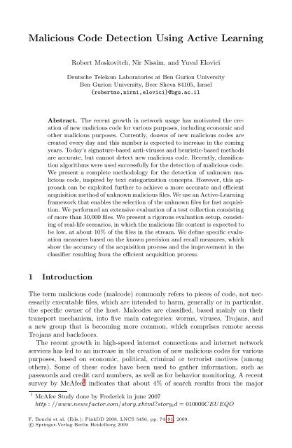
<strong>Malicious</strong> <strong>Code</strong> <strong>Detection</strong> <strong>Using</strong> <strong>Active</strong> <strong>Learning</strong><br />
Robert Moskovitch, Nir Nissim, and Yuval Elovici<br />
Deutsche Telekom Laboratories at Ben Gurion University<br />
Ben Gurion University, Beer Sheva 84105, Israel<br />
{robertmo,nirni,elovici}@bgu.ac.il<br />
Abstract. The recent growth in network usage has motivated the creation<br />
<strong>of</strong> new malicious code for various purposes, including economic and<br />
other malicious purposes. Currently, dozens <strong>of</strong> new malicious codes are<br />
created every day and this number is expected to increase in the coming<br />
years. Today’s signature-based anti-viruses and heuristic-based methods<br />
are accurate, but cannot detect new malicious code. Recently, classification<br />
algorithms were used successfully for the detection <strong>of</strong> malicious code.<br />
We present a complete methodology for the detection <strong>of</strong> unknown malicious<br />
code, inspired by text categorization concepts. However, this approach<br />
can be exploited further to achieve a more accurate and efficient<br />
acquisition method <strong>of</strong> unknown malicious files. We use an <strong>Active</strong>-<strong>Learning</strong><br />
framework that enables the selection <strong>of</strong> the unknown files for fast acquisition.<br />
We performed an extensive evaluation <strong>of</strong> a test collection consisting<br />
<strong>of</strong> more than 30,000 files. We present a rigorous evaluation setup, consisting<br />
<strong>of</strong> real-life scenarios, in which the malicious file content is expected to<br />
be low, at about 10% <strong>of</strong> the files in the stream. We define specific evaluation<br />
measures based on the known precision and recall measures, which<br />
show the accuracy <strong>of</strong> the acquisition process and the improvement in the<br />
classifier resulting from the efficient acquisition process.<br />
1 Introduction<br />
The term malicious code (malcode) commonly refers to pieces <strong>of</strong> code, not necessarily<br />
executable files, which are intended to harm, generally or in particular,<br />
the specific owner <strong>of</strong> the host. Malcodes are classified, based mainly on their<br />
transport mechanism, into five main categories: worms, viruses, Trojans, and<br />
a new group that is becoming more common, which comprises remote access<br />
Trojans and backdoors.<br />
The recent growth in high-speed internet connections and internet network<br />
services has led to an increase in the creation <strong>of</strong> new malicious codes for various<br />
purposes, based on economic, political, criminal or terrorist motives (among<br />
others). Some <strong>of</strong> these codes have been used to gather information, such as<br />
passwords and credit card numbers, as well as for behavior monitoring. A recent<br />
survey by McAfee 1 indicates that about 4% <strong>of</strong> search results from the major<br />
1 McAfee Study done by Frederick in june 2007<br />
http : //www.newsfactor.com/story.xhtmlstory id = 010000CEUEQO<br />
F. Bonchi et al. (Eds.): PinkDD 2008, LNCS 5456, pp. 74–91, 2009.<br />
c○ Springer-Verlag Berlin Heidelberg 2009
<strong>Malicious</strong> <strong>Code</strong> <strong>Detection</strong> <strong>Using</strong> <strong>Active</strong> <strong>Learning</strong> 75<br />
search engines on the web contain malicious code. Additionally, Shin et al. [1]<br />
found that above 15% <strong>of</strong> the files in the KaZaA network contained malicious<br />
code. Thus, we assume that the proportion <strong>of</strong> malicious files in real life is about<br />
or less than 10%, but we also consider other options <strong>of</strong> malicious files proportions<br />
through the imbalanced problem that will be briefly explain in the next section.<br />
Current anti-virus technology is primarily based on two approaches. Signaturebased<br />
methods, which rely on the identification <strong>of</strong> unique strings in the binary<br />
code, while being very precise, are useless against unknown malicious code. The<br />
second approach involves heuristic-based methods, which are based on rules<br />
defined by experts, which define a malicious behavior, or a benign behavior, in<br />
order to enable the detection <strong>of</strong> unknown malcodes [2]. Other proposed methods<br />
include behavior blockers, which attempt to detect sequences <strong>of</strong> events in<br />
operating systems, and integrity checkers, which periodically check for changes<br />
in files and disks. However, besides the fact that these methods can be bypassed<br />
by viruses, their main drawback is that, by definition, they can only detect the<br />
presence <strong>of</strong> a malcode after the infected program has been executed, unlike the<br />
signature-based methods, including the heuristic-based methods, which are very<br />
time-consuming and have a relatively high false alarm rate.<br />
Recently, classification algorithms were employed to automate and extend the<br />
idea <strong>of</strong> heuristic-based methods. As we will describe in more detail shortly, the<br />
binary code <strong>of</strong> a file is represented by n-grams, and classifiers are applied to<br />
learn patterns in the code and classify large amounts <strong>of</strong> data. A classifier is a<br />
rule set which is learnt from a given training-set, including examples <strong>of</strong> classes,<br />
both malicious and benign files in our case. Recent studies, which we survey in<br />
the next section, have shown that this is a very successful strategy.<br />
Another problem which is troubling the anti virus community is the acquisition<br />
<strong>of</strong> new malicious files, which is very important to detect as quickly as possible.<br />
This is <strong>of</strong>ten done by using honey-pots. Another option is to scan the traffic at<br />
the internet service provider, if accessible, to increase the probability <strong>of</strong> detection<br />
<strong>of</strong> a new malcode. However, the main challenge in both options is to scan all the<br />
files efficiently, especially when scanning internet node (router) traffic.<br />
We present a methodology for malcode categorization based on concepts from<br />
text categorization. We present an extensive and rigorous evaluation <strong>of</strong> many<br />
factors in the methodology, based on SVM classifiers using three types <strong>of</strong> kernels.<br />
The evaluation is based on a test collection containing more than 30,000 files.<br />
In this study we focus on the problem <strong>of</strong> efficiently scanning and acquiring new<br />
malicious code in a stream <strong>of</strong> executable files using <strong>Active</strong> Learners. We have<br />
shown that by using an inteligent acquisition <strong>of</strong> executables it is possible to<br />
acquire only small part <strong>of</strong> the files in the stream and still achieve significant<br />
improvement in the detection performance, an improvement that contributes to<br />
the learner’s updatability in light <strong>of</strong> the new files over the net. while also saves<br />
time and money as will be explained later.<br />
We start with a survey <strong>of</strong> previous relevant studies. We describe the methods<br />
we used to represent the executable files. We present our approach <strong>of</strong> acquiring
76 R. Moskovitch, N. Nissim, and Y. Elovici<br />
new malcodes using <strong>Active</strong> <strong>Learning</strong> and perform a rigorous evaluation. Finally,<br />
we present our results and discuss them.<br />
2 Background<br />
2.1 Detecting Malcodes via Data Mining<br />
Over the past five years, several studies have investigated the option <strong>of</strong> detecting<br />
unknown malcode based on its binary code. Schultz et al. [3] were the first to<br />
introduce the idea <strong>of</strong> applying machine learning (ML) methods for the detection<br />
<strong>of</strong> different malcodes based on their respective binary codes. They used three<br />
different feature extraction (FE) approaches – program header, string features,<br />
and byte sequence features – in which they applied four classifiers – a signaturebased<br />
method (anti-virus), Ripper, a rule-based learner, Naive Bayes, and Multi-<br />
Naive Bayes. This study found that all the ML methods were more accurate<br />
than the signature-based algorithm. The ML methods were more than twice as<br />
accurate, with the out-performing method being Naive Bayes, using strings, or<br />
Multi-Naive Bayes using byte sequences.<br />
Abou-Assaleh et al. [4] introduced a framework that used the common n-gram<br />
(CNG) method and the k nearest neighbor (KNN) classifier for the detection <strong>of</strong><br />
malcodes. For each class, malicious and benign, a representative pr<strong>of</strong>ile was constructed<br />
and assigned a new executable file. This executable file was compared<br />
with the pr<strong>of</strong>iles and matched to the most similar. Two different datasets were<br />
used: the I-worm collection, which consisted <strong>of</strong> 292 Windows internet worms, and<br />
the win32 collection, which consisted <strong>of</strong> 493 Windows viruses. The best results<br />
were achieved using 3-6 n-grams and a pr<strong>of</strong>ile <strong>of</strong> 500-5000 features.<br />
Kolter and Malo<strong>of</strong> [5] presented a collection that included 1971 benign and<br />
1651 malicious executables files. N-grams were extracted and 500 were selected<br />
using the information gain measure [6]. The vector <strong>of</strong> n-gram features was binary,<br />
presenting the presence or absence <strong>of</strong> a feature in the file and ignoring the<br />
frequency <strong>of</strong> feature appearances. In their experiment, they trained several classifiers:<br />
IBK (KNN), a similarity based classifier called TFIDF classifier, Naive<br />
Bayes, SVM (SMO), and Decision tree (J48), the last three <strong>of</strong> which were also<br />
boosted. Two main experiments were conducted on two different datasets, a<br />
small collection and a large collection. The small collection consisted <strong>of</strong> 476 malicious<br />
and 561 benign executables and the larger collection <strong>of</strong> 1651 malicious<br />
and 1971 benign executables. In both experiments, the four best-performing<br />
classifiers were Boosted J48, SVM, boosted SVM, and IBK. Boosted J48 outperformed<br />
the others, The authors indicated that the results <strong>of</strong> their n-gram<br />
study were better than those presented by Schultz and Eskin [3].<br />
Recently, Kolter and Malo<strong>of</strong> [7] reported an extension <strong>of</strong> their work, in which<br />
they classified malcodes into families (classes) based on the functions in their respective<br />
payloads. In the categorization task <strong>of</strong> multiple classifications, the best<br />
results were achieved for the classes: mass mailer, backdoor, and virus (no benign<br />
classes). In attempts to estimate their ability to detect malicious codes based on<br />
their issue dates, these classifiers were trained on files issued before July 2003,
<strong>Malicious</strong> <strong>Code</strong> <strong>Detection</strong> <strong>Using</strong> <strong>Active</strong> <strong>Learning</strong> 77<br />
and then tested on 291 files issued from that point in time through August<br />
2004. The results were, as expected, not as good as those <strong>of</strong> previous experiments.<br />
These results indicate the importance <strong>of</strong> maintaining such a training set<br />
through the acquisition <strong>of</strong> new executables, in order to cope with unknown new<br />
executables.<br />
Henchiri and Japkowicz [8] presented a hierarchical feature selection approach<br />
which makes possible the selection <strong>of</strong> n-gram features that appear at rates above<br />
a specified threshold in a specific virus family, as well as in more than a minimal<br />
amount <strong>of</strong> virus classes (families). They applied several classifiers, ID3, J48 Naive<br />
Bayes, SVM- and SMO, to the dataset used by Schultz et al. [3] and obtained<br />
results that were better than those obtained using a traditional feature selection,<br />
as presented in [3], which focused mainly on 5-grams. However, it is not clear<br />
whether these results are reflective more <strong>of</strong> the feature selection method or <strong>of</strong><br />
the number <strong>of</strong> features that were used.<br />
Moskovitch et al [9] presented a test collection consisting <strong>of</strong> more than 30,000<br />
executable files, which is the largest known to us. They performed a wide evaluation<br />
consisting <strong>of</strong> five types <strong>of</strong> classifiers and focused on the imbalance problem<br />
in real life conditions, in which the percentage <strong>of</strong> malicious files is less than 10%,<br />
based on recent surveys. After evaluating the classifiers on varying percentages<br />
<strong>of</strong> malicious files in the training set and test sets, it was shown to achieve the<br />
optimal results when having similar proportions in the training set as expected<br />
in the test set.<br />
2.2 <strong>Active</strong> <strong>Learning</strong> and Selective Sampling<br />
A major challenge in supervised learning is labeling the examples in the dataset.<br />
Often the labeling is expensive since it is done manually by human experts.<br />
Labeled examples are crucial in order to train a classifier, and we would therefore<br />
like to reduce the number <strong>of</strong> labeling requirements. The <strong>Active</strong> <strong>Learning</strong> (AL)<br />
approach proposes a method which asks actively for labeling <strong>of</strong> specific examples,<br />
based on their potential contribution to the learning process.<br />
AL is roughly divided into two major approaches: the membership queries [10]<br />
and the selective-sampling approach [11]. In the membership queries approach<br />
the learner constructs artificial examples from the problem space, then asks for<br />
its label from the expert, and finally learns from it and so forth, in an attempt<br />
to cover the problem space and to have a minimal number <strong>of</strong> examples that<br />
represent most <strong>of</strong> the types among the existing examples. However, a potential<br />
practical problem in this approach is requesting a label for a nonsense example.<br />
The selective-sampling approach usually comprises a pool-based sampling, in<br />
which the learner is given a large set <strong>of</strong> unlabeled data (pool) from which it<br />
iteratively selects the most informative and contributive examples for labeling<br />
and learning, based on which it is carefully selects the next examples, until it<br />
meets stopping criteria.<br />
Studies in several domains successfully applied active learning in order to<br />
reduce the effort <strong>of</strong> labeling examples. Unlike in random learning, in which a<br />
classifier is trained on a pool <strong>of</strong> labeled examples, the classifier actively indicates
78 R. Moskovitch, N. Nissim, and Y. Elovici<br />
the specific examples that should be labeled, which are commonly the most<br />
informative examples for the training task. Two AL methods were considered in<br />
our experiments: Simple-Margin Tong and Koller [12] Error-Reduction Roy and<br />
McCallum [13].<br />
2.3 Acquisition <strong>of</strong> New <strong>Malicious</strong> <strong>Code</strong> <strong>Using</strong> <strong>Active</strong> <strong>Learning</strong><br />
As we presented briefly earlier the option <strong>of</strong> acquiring new malicious files from<br />
the web and internet services providers is essential for fast detection and updating<br />
<strong>of</strong> the anti-viruses, as well as updating <strong>of</strong> the classifiers. However, manually<br />
inspecting each potentially malicious file is time-consuming, and <strong>of</strong>ten done by<br />
human experts. We propose using <strong>Active</strong> <strong>Learning</strong> as a selective sampling approach<br />
based on a static analysis <strong>of</strong> malicious code, in which the active learner<br />
identifies new examples which are expected to be unknown. Moreover, the active<br />
learner is expected to present a ranked list <strong>of</strong> the most informative examples,<br />
which are probably the most different from what currently is known.<br />
3 Methods<br />
3.1 Text Categorization<br />
To detect and acquire unknown malicious code, we suggest implementing wellstudied<br />
concepts from the information retrieval (IR) and more specific text categorization<br />
domain. In execution <strong>of</strong> our task, binary files (executables) are parsed<br />
and n-gram terms are extracted. Each n-gram term in our task is analogous to<br />
words in the textual domain. Here are descriptions <strong>of</strong> the IR concepts used in<br />
this study. Salton and Weng [14] presented the vector space model to represent a<br />
textual file as a bag-<strong>of</strong>-words. After parsing the text and extracting the words, a<br />
vocabulary <strong>of</strong> the entire collection <strong>of</strong> words is constructed. Each <strong>of</strong> these words<br />
may appear zero to multiple times in a document. A vector <strong>of</strong> terms is created,<br />
such that each index in the vector represents the term frequency (TF) in<br />
the document. Equation (1) shows the definition <strong>of</strong> a normalized TF, in which<br />
the term frequency is divided by the maximal appearing term in the document<br />
with values in the range <strong>of</strong> [0-1]. Another common representation is the TF Inverse<br />
Document Frequency (TFIDF), which combines the frequency <strong>of</strong> a term<br />
in the document (TF) and its frequency in the documents collection, as shown<br />
in Equation (2), in which the term’s (normalized) TF value is multiplied by the<br />
IDF = log( N n<br />
), where N is the number <strong>of</strong> documents in the entire file collection<br />
and n is the number <strong>of</strong> documents in which the term appears.<br />
TF =<br />
term frequency<br />
max(term frequency in document)<br />
(1)<br />
TFIDF = TF ∗ log(DF),<br />
Where DF = N n<br />
(2)
3.2 Data Set Creation<br />
<strong>Malicious</strong> <strong>Code</strong> <strong>Detection</strong> <strong>Using</strong> <strong>Active</strong> <strong>Learning</strong> 79<br />
We created a dataset <strong>of</strong> malicious and benign executables for the Windows operating<br />
system, which is the most commonly used and attacked. To the best <strong>of</strong><br />
our knowledge, this collection is the largest ever assembled. We acquired the malicious<br />
files from the VX Heaven website 2 , having 7688 malicious files. To identify<br />
the files, we used the Kaspersky anti-virus and the Windows version <strong>of</strong> the<br />
Unix ’file’ command for file type identification. The files in the benign set, including<br />
executable and Dynamic Linked Library (DLL) files, were gathered from machines<br />
running the Windows XP operating system, which is currently considered<br />
the most used, on our campus. The benign set contained 22,735 files, which were<br />
reported by the Kaspersky anti-virus 3 program as being completely virus-free.<br />
3.3 Data Preparation and Feature Selection<br />
We parsed the binary code <strong>of</strong> the executable files using several n-gram lengths<br />
moving windows, denoted by n. Vocabularies <strong>of</strong> 16,777,216, 1,084,793,035,<br />
1,575,804,954, and 1,936,342,220, for 3-gram, 4-gram, 5-gram and 6-gram, respectively,<br />
were extracted. Later the TF and TFIDF representation were calculated<br />
for each n-gram in each file.<br />
In machine learning applications, the large number <strong>of</strong> features (many <strong>of</strong> which<br />
do not contribute to the accuracy and may even decrease it) in many domains<br />
presents a huge problem. Moreover, in our task a reduction in the amount <strong>of</strong><br />
features is crucial for practical reasons, but must be performed while simultaneously<br />
maintaining a high level <strong>of</strong> accuracy. This is due to the fact that, as shown<br />
earlier, the vocabulary size may exceed billions <strong>of</strong> features, far more than can<br />
be processed by any feature selection tool within a reasonable period <strong>of</strong> time.<br />
Additionally, it is important to identify those terms that appear in most <strong>of</strong> the<br />
files, in order to avoid zeroed representation vectors. Thus, initially the features<br />
having the highest DF value Equation (2) were extracted.<br />
Based on the DF measure, two sets were selected, the top 5,500 terms and the<br />
top 1,000-6,500 terms. The set <strong>of</strong> top 1000 to 6,500 set <strong>of</strong> features was inspired<br />
by the removal <strong>of</strong> stop-words, as <strong>of</strong>ten done in information retrieval for common<br />
words. Later, feature selection methods were applied to each <strong>of</strong> these two sets.<br />
Since it is not the focus <strong>of</strong> this paper, we will describe the feature selection<br />
preprocessing very briefly. We used a filters approach, in which the measure<br />
was independent <strong>of</strong> any classification algorithm, to compare the performances<br />
<strong>of</strong> the different classification algorithms. In a filters approach, a measure is used<br />
to quantify the correlation <strong>of</strong> each feature to the class (malicious or benign)<br />
and estimate its expected contribution to the classification task. Three feature<br />
selection measures were used: as a baseline we used the document frequency<br />
measure DF (Equation 2), and additionally the Gain Ratio (GR) [6] and Fisher<br />
Score [15]. Eventually the top 50, 100, 200 300, 1000, 1500 and 2000 were selected<br />
from each feature selection.<br />
2 http://vx.netlux.org<br />
3 http://www.kaspersky.com
80 R. Moskovitch, N. Nissim, and Y. Elovici<br />
3.4 Support Vector Machines<br />
We employed the SVM classification algorithm using three different kernel functions,<br />
in a supervised learning approach. We briefly introduce the SVM classification<br />
algorithm and the principles and implementation <strong>of</strong> <strong>Active</strong> <strong>Learning</strong><br />
that we used in this study. SVM is a binary classifier which finds a linear hyperplane<br />
that separates the given examples into the two given classes. Later an<br />
extension that enables handling multiclass classification was developed. SVM is<br />
widely known for its capacity to handle a large amount <strong>of</strong> features, such as text,<br />
as was shown by Joachims [16]. We used the Lib-SVM implementation <strong>of</strong> Chang<br />
[17] that also handles multiclass classification.<br />
Given a training set, in which an example is a vector x i =,<br />
where f i is a feature, and labeled by y i = -1,+1, the SVM attempts to specify<br />
a linear hyperplane that has the maximal margin, defined by the maximal (perpendicular)<br />
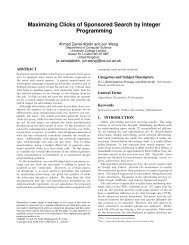
distance between the examples <strong>of</strong> the two classes. Fig. 1 illustrates<br />
a two dimensional space, in which the examples are located according to their<br />
features and the hyperplane splits them according to their label.<br />
Fig. 1. An SVM that separates the training set into two classes, having maximal margin<br />
in a two dimensional space<br />
The examples lying closest to the hyperplane are the ”supporting vectors” W,<br />
the Normal <strong>of</strong> the hyperplane, is a linear combination <strong>of</strong> the most important examples<br />
(supporting vectors), multiplied by LaGrange multipliers (alphas). Since<br />
the dataset in the original space <strong>of</strong>ten cannot be linearly separated, a kernel
<strong>Malicious</strong> <strong>Code</strong> <strong>Detection</strong> <strong>Using</strong> <strong>Active</strong> <strong>Learning</strong> 81<br />
function K is used. SVM actually projects the examples into a higher dimensional<br />
space in order to create linear separation <strong>of</strong> the examples. Note that when<br />
the kernel function satisfies Mercer’s condition, as was explained by Burges [18],<br />
K can be written as shown in Equation (3), where φ is a function that maps the<br />
example from the original feature space into a higher dimensional space, while<br />
K relies on ”inner product” between the mappings <strong>of</strong> examples x 1 ,x 2 .Forthe<br />
general case, the SVM classifier will be in the form shown in Equation (4), while<br />
n is the number <strong>of</strong> examples in training set, and w is defined in Equation (5).<br />
K(x 1 ,x 2 )=φ(x 1 ) · φ(x 2 ) (3)<br />
F (x) =sign(W · φ(x)) = sign(<br />
W =<br />
n∑<br />
α i y i K(x i ,x)) (4)<br />
1<br />
n∑<br />
α i y i φ(x i ) (5)<br />
1<br />
Two commonly used kernel functions were used: Polynomial kernel, as shown<br />
in Equation (6), creates polynomial values <strong>of</strong> degree p, where the output depends<br />
on the direction <strong>of</strong> the two vectors, examples x 1 ,x 2 , in the original problem<br />
space. Note that a private case <strong>of</strong> a polynomial kernel, having p=1, is actually<br />
the Linear kernel. Radial Basis Function (RBF), as shown in Equation (7), in<br />
which a Gaussian is used as the RBF and the output <strong>of</strong> the kernel depends on<br />
the Euclidean distance <strong>of</strong> examples x 1 ,x 2 .<br />
K(x 1 ,x 2 )=(x 1 · x 2 ) p (6)<br />
K(x 1 ,x 2 )=e( − |x 1 − x 2 | 2<br />
2σ 2 ) (7)<br />
3.5 <strong>Active</strong> <strong>Learning</strong><br />
In this study we implemented two selective sampling (pool-based) AL methods:<br />
the Simple Margin presented by Tong and Koller [12] ,and Error Reduction<br />
presented by Roy and McCallum [13].<br />
Simple-Margin. This method is directly oriented to the SVM classifier. As<br />
was explained in the section 3.4, by using a kernel function, the SVM implicitly<br />
projects the training examples into a different (usually higher dimensional)<br />
feature space, denoted by F. In this space there is a set <strong>of</strong> hypotheses that are<br />
consistent with the training-set, meaning that they create linear separation <strong>of</strong><br />
the training-set. This set <strong>of</strong> consistent hypotheses is called Version-Space (VS).
82 R. Moskovitch, N. Nissim, and Y. Elovici<br />
From among the consistent hypotheses, the SVM then identifies the best hypothesis<br />
that has the maximal margin. Thus, the motivation <strong>of</strong> the Simple-<br />
Margin AL method is to select those examples from the pool, so that these will<br />
reduce the number <strong>of</strong> hypotheses in the VS, in an attempt to achieve a situation<br />
where VS contains the most accurate and consistent hypotheses. Calculating the<br />
VS is complex and impractical when large datasets are considered, and therefore<br />
this method is oriented through simple heuristics that are based on the relation<br />
between the VS and the SVM with the maximal margin. Practically, examples<br />
that lie closest to the separating hyperplane (inside the margin) are more likely<br />
to be informative and new to the classifier, and thus will be selected for labeling<br />
and acquisition.<br />
Error-Reduction. The Error Reduction method is more general and can be<br />
applied to any classifier that can provide probabilistic values for its classification<br />
decision. Based on the estimation <strong>of</strong> the expected error, which is achieved<br />
through adding an example into the training-set with each label, the example<br />
that is expected to lead to the minimal expected error will be selected and<br />
labeled. Since the real future error rates are unknown, the learner utilizes its<br />
current classifier in order to estimate those errors.<br />
In the beginning <strong>of</strong> an AL trial, an initial classifier P ˆ D (y|x) is trained over a<br />
randomly selected initial set D. For every optional label yɛY (<strong>of</strong> every example<br />
x in the pool P) the algorithm induces a new classifier Pˆ<br />
D ′(y|x) trainedon<br />
the extended training set D ′ = D +(x, y) Thus (in our binary case, malicious<br />
and benign are the only optional labels) for every example x there are two<br />
classifiers, each one for each label. Then for each one <strong>of</strong> the example’s classifiers<br />
the future expected generalization error is estimated using a log-loss function,<br />
shown in Equation 8. The log-loss function measures the error degree <strong>of</strong> the<br />
current classifier over all the examples in the pool, where this classifier represents<br />
the induced classifier as a result <strong>of</strong> selecting a specific example from the pool and<br />
adding it to the training set, having a specific label. Thus, for every example xɛP<br />
we actually have two future generalization errors (one for each optional label as<br />
was calculated in Equation (8)). Finally, an average is calculated for the two<br />
errors, which is called the self-estimated average error, based on Equation (9).<br />
It can be understood that it is built <strong>of</strong> the weighted average so that the<br />
weight <strong>of</strong> each error <strong>of</strong> example x with label y is given by the prior probability<br />
<strong>of</strong> the initial classifier to classify correctly example x with label y. Finally, the<br />
example x with the lowest expected self-estimated error is chosen and added to<br />
the training set. In a nutshell, an example will be chosen from the pool only if it<br />
dramatically improves the confidence <strong>of</strong> the current classifier more than all the<br />
examples in the pool (means lower estimated error).<br />
EP ˆ = 1 ∑ ∑<br />
Pˆ<br />
D ′ D ′(y|x) ·|log( P<br />
|P |<br />
ˆ D ′(y|x))| (8)<br />
xɛX yɛY<br />
∑<br />
Pˆ<br />
D (y|x) · EP ˆ D<br />
(9)<br />
′<br />
yɛY
<strong>Malicious</strong> <strong>Code</strong> <strong>Detection</strong> <strong>Using</strong> <strong>Active</strong> <strong>Learning</strong> 83<br />
4 Evaluation<br />
To evaluate the use <strong>of</strong> AL in the task <strong>of</strong> efficient acquisition <strong>of</strong> new files, we<br />
defined specific measures derived from the experimental objectives. The first<br />
experimental objective was to determine the optimal settings <strong>of</strong> the term representation<br />
(TF or TFIDF), n-grams representation (3, 4, 5 or 6), the best global<br />
range (top 5500 or top 1000-6500) and feature selection method (DF, FS or GR),<br />
and the top selection (50, 100, 200, 300, 1000, 1500 or 2000). After determining<br />
the optimal settings, we performed a second experiment to evaluate our proposed<br />
acquisition process using the two AL methods.<br />
4.1 Evaluation Measures<br />
For evaluation purposes, we measured the True Positive Rate (TPR) measure,<br />
which is the number <strong>of</strong> positive instances classified correctly, as shown in Equation<br />
(10), False Positive Rate (FPR), which is the number <strong>of</strong> negative instances<br />
misclassified Equation (10), and the Total Accuracy, which measures the number<br />
<strong>of</strong> absolutely correctly classified instances, either positive or negative, divided<br />
by the entire number <strong>of</strong> instances, shown in Equation (11).<br />
TPR =<br />
|TP|<br />
|TP + FN|<br />
,FPR=<br />
|FP|<br />
|FP + TN|<br />
(10)<br />
Total Accuracy =<br />
|TP + TN|<br />
|TP + FP + TN + FN|<br />
(11)<br />
4.2 Evaluation Measures for the Acquisition Process<br />
In this study we wanted to evaluate the acquisition performance <strong>of</strong> the <strong>Active</strong>-<br />
Learner from a stream <strong>of</strong> files presented by the test set, containing benign and<br />
malicious executables, including new (unknown) and not-new files. Actually, the<br />
task here is to evaluate the capability <strong>of</strong> the module to acquire the new files in<br />
the test set, which cannot be evaluated only by the common measures evaluated<br />
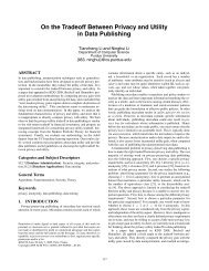
earlier. Figure 2 illustrates the evaluation scheme describing the varying<br />
contents <strong>of</strong> the test set and Acquisition set that will be explained shortly. The<br />
datasets contain two types <strong>of</strong> files: <strong>Malicious</strong> (M) and Benign (B). While the<br />
<strong>Malicious</strong> region is presented as a bit smaller, it is actually significantly smaller.<br />
These datasets contain varying files partially known to the classifier, from the<br />
training set, and a larger portion <strong>of</strong> New (N) files, which are expected to be acquired<br />
by the <strong>Active</strong> Learner, illustrated by a circle. The active learner acquires<br />
from the stream part <strong>of</strong> the files, illustrated by the Acquired (A) circle. Ideally<br />
the Acquired circle will be identical to the New circle.
84 R. Moskovitch, N. Nissim, and Y. Elovici<br />
To define the evaluation measures, we define the resultant regions in the evaluation<br />
scheme by:<br />
– A ∩ M\N - The <strong>Malicious</strong> files Acquired, but not New.<br />
– A ∩ M ∩ N - The <strong>Malicious</strong> files Acquired and New.<br />
– M ∩ N\A- The New <strong>Malicious</strong> files, but not Acquired.<br />
– A ∩ B\N - The Benign files Acquired, but not New.<br />
– A ∩ B ∩ N - The Benign files Acquired and New.<br />
Fig. 2. An illustration <strong>of</strong> the evaluation scheme, including the <strong>Malicious</strong> (M) and Benign<br />
(B) Files, the New files to acquire (N) and the actual Acquired (A) files<br />
For the evaluation <strong>of</strong> the said scheme we used the known Precision and Recall<br />
measures, <strong>of</strong>ten used in information retrieval and text categorization. We first<br />
define the traditional precision and recall measures. Equation (12) represents the<br />
Precision, which is the proportion <strong>of</strong> the accurately classified examples among<br />
the classified examples. Equation (13) represents the Recall measure, which is<br />
the proportion <strong>of</strong> the classified examples from a specific class in the entire class<br />
examples.<br />
P recision =<br />
|{Relevant examples}| ∩ |{Classified examples}|<br />
|{Classified examples}|<br />
(12)<br />
Recall =<br />
|{Relevant examples}| ∩ |{Classified examples}|<br />
|{Relevant examples}|<br />
(13)
<strong>Malicious</strong> <strong>Code</strong> <strong>Detection</strong> <strong>Using</strong> <strong>Active</strong> <strong>Learning</strong> 85<br />
As we will elaborate later, the acquisition evaluation set will contain both<br />
malicious and benign files, partially new (were not in the training set) and partially<br />
not-new (appeared in the training set), and thus unknown to the classifier.<br />
To evaluate the selective method we define here the precision and recall measures<br />
in the context <strong>of</strong> our problem. Corresponding to the evaluation scheme<br />
presented in Figure 2, the precision new benign is defined in Equation (14) by<br />
the proportion among the new benign files which were acquired and the acquired<br />
benign files. Similarly the precision new malicious is defined in Equation (15).<br />
The recall new benign is defined in Equation (16) by how many new benign<br />
files in the stream were acquired from the entire set <strong>of</strong> new benign in the stream.<br />
T herecall new malicious is defined similarly in Equation (17).<br />
P recision new benign = A ∩ B ∩ N<br />
A ∩ B<br />
P recision new malicious = A ∩ M ∩ N<br />
A ∩ M<br />
Recall new benign = A ∩ B ∩ N<br />
N ∩ B<br />
(14)<br />
(15)<br />
(16)<br />
Recall new malicious = A ∩ M ∩ N<br />
(17)<br />
N ∩ M<br />
The acquired examples are important for the incremental improvement <strong>of</strong><br />
theclassifier;The<strong>Active</strong>Learneracquires the new examples which are mostly<br />
important for the improvement <strong>of</strong> the classifier, but not all the new examples are<br />
acquired, especially these which the classifier is certain on their classification.<br />
However, we would like to be aware <strong>of</strong> any new files (especially malicious) in<br />
order to examine them and add them to the repository. This set <strong>of</strong> files are<br />
the New and not Acquired (N\A), thus, we would like to measure the accuracy<br />
<strong>of</strong> the classification <strong>of</strong> these files to make sure that the classifier classified them<br />
correctly. This is done using the Accuracy measure as presented in Equation (11)<br />
on the subset defined by (N\A), where for example |TP(N\A)| is the number<br />
<strong>of</strong> malicious executables that were labeled correctly as malicious, out <strong>of</strong> the unacquired<br />
new examples. In addition we measured the classification accuracy <strong>of</strong><br />
the classifier in classifying examples which were not new and not acquired. Thus,<br />
using again the Accuracy measure (Equation (11)) for the ¬(N ∪ A) defines our<br />
evaluation measure.<br />
5 Experiments and Results<br />
5.1 Experiment 1<br />
To determine the best settings <strong>of</strong> the file representation and the feature selection<br />
we performed a wide and comprehensive set <strong>of</strong> evaluation runs, including all<br />
the combinations <strong>of</strong> the optional settings for each <strong>of</strong> the aspects, amounting to
86 R. Moskovitch, N. Nissim, and Y. Elovici<br />
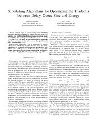
Fig. 3. The results <strong>of</strong> the global selection, term representation, and n-grams, in which<br />
the Top 5500 global selection having the TF representation is outperforming, especially<br />
with 5-grams<br />
1536 runs in a 5-fold cross validation format for all the three kernels. Note that<br />
the files in the test-set were not in the training-set presenting unknown files to<br />
the classifier.<br />
Global Feature Selection vs n-grams. Figure 3 presents the mean accuracy<br />
<strong>of</strong> the combinations <strong>of</strong> the term representations and n-grams. The top 5,500<br />
features outperformed with the TF representation and the 5-gram in general. The<br />
out-performing <strong>of</strong> the TF has meaningful computational advantages, on which<br />
we will elaborate in the Discussion. In general, mostly the 5-grams outperformed<br />
the others.<br />
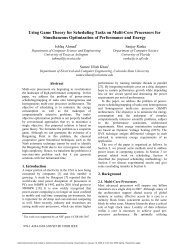
Feature Selections and Top Selections. Figure 4 presents the mean accuracy<br />
<strong>of</strong> the three feature selection methods and the seven top selections. For<br />
fewer features, the FS outperforms, while above the Top 300 there was not much<br />
difference. However, in general the FS outperformed the other methods. For all<br />
the three feature selection methods there is a decrease in the accuracy when<br />
using above Top 1000 features.<br />
Classifiers. After determining the best configuration <strong>of</strong> 5-Grams, Global top<br />
5500, TF representation, Fischer score, and Top300, we present in Table 1 the<br />
results <strong>of</strong> each SVM kernel. The RBF kernel out-performed the others and had<br />
a low false positive rate, while the other kernels also perform very well.
<strong>Malicious</strong> <strong>Code</strong> <strong>Detection</strong> <strong>Using</strong> <strong>Active</strong> <strong>Learning</strong> 87<br />
Fig. 4. The accuracy increased as more features were used, while in general the FS<br />
outperformed the other measures<br />
Table 1. The RBF kernel outperformed while maintaining a low level <strong>of</strong> false positive<br />
Kernel Accuracy FP FN<br />
SVM-LIN 0.921 0.033 0.214<br />
SVM-POL 0.852 0.014 0.544<br />
SVM-RBF 0.939 0.029 0.154<br />
5.2 Experiment 2. Files Acquisition<br />
In the second experiment we used the optimal settings from experiment 1, applying<br />
only the RBF kernel which outperformed (Table 1). In this set <strong>of</strong> experiments,<br />
we set an imbalanced representation <strong>of</strong> malicious-benign proportions in the testset<br />
to reflect real life conditions <strong>of</strong> 10% malicious files in the stream, based on the<br />
information provided in the Introduction. In a previous study [9] we found that<br />
the optimal proportions in such scenario are similar settings in the training set.<br />
The Dataset includes 25000 executables (22,500 benign, 2500 malicious), having<br />
10% malicious and: 90% benign contents as in real life conditions. The evaluation<br />
test collection included several components: Training-Set, Acquisition-Set<br />
(Stream), and Test-set. The Acquisition-set consisted <strong>of</strong> benign and malicious<br />
examples, including known executables (that appeared in the training set) and
88 R. Moskovitch, N. Nissim, and Y. Elovici<br />
unknown executables (which did not appear in the training set) and the Test-set<br />
included the entire Data-set. These sets were used in the following steps <strong>of</strong> the<br />
experiment:<br />
1. A Learner is trained on the Training-Set.<br />
2. The model is tested on the Test-Set to measure the initial accuracy.<br />
3. A stream <strong>of</strong> files is introduced to the <strong>Active</strong> Learner, which asks selectively<br />
for labeling <strong>of</strong> specific files, which are acquired.<br />
4. After acquiring all the new informative examples, the Learner is trained<br />
on the new Training-Set.<br />
5. The Learner is tested on the Test-Set.<br />
We applied the learners in each step using 2 different variation <strong>of</strong> cross validation<br />
for each AL method. For the Simple-Margin we used variation <strong>of</strong> 10-fold<br />
cross validation. Thus, the Acquisition Set (stream) contained part <strong>of</strong> the folds<br />
in the Training Set and the Test Set, which was used for evaluation prior to the<br />
Acquisition phase and after, contained all the folds.<br />
Simple-Margin AL method - We applied the Simple Margin <strong>Active</strong> Learner<br />
in the experimental setup presented earlier. Table 2 presents the mean results<br />
<strong>of</strong> the cross validation experiment. Both the Benign and the <strong>Malicious</strong> Precision<br />
were very high, above 99%, which means that most <strong>of</strong> the acquired files were<br />
indeed new. The Recall measures were quite low, especially the Benign Recall.<br />
This can be explained by the need <strong>of</strong> the <strong>Active</strong> Learner to improve the accuracy.<br />
An interesting fact is the difference in the Recall <strong>of</strong> the <strong>Malicious</strong> and the<br />
Benign, which can be explained by the varying proportions in the training set,<br />
which was 10% malicious. The classification accuracy <strong>of</strong> the new examples that<br />
were not acquired was very high as well, being close to 99%, which was also the<br />
classification accuracy <strong>of</strong> the not new, which was 100%. However, the improvement<br />
between the Initial and Final accuracy was significant, which shows the<br />
importance and the efficiency in the acquisition process.<br />
Table 2. The Simple-Margin acquisition performance<br />
Measure Simple Margin Performance<br />
Precision Benign 99.81%<br />
Precision <strong>Malicious</strong> 99.22%<br />
Recall Benign 33.63%<br />
Recall <strong>Malicious</strong> 82.82%<br />
Accuracy(N\A) 98.90%<br />
Accuracy¬(N ∩ A) 100%<br />
Initial Accuracy on Test-Set 86.63%<br />
Final Accuracy on Test-Set 92.13%<br />
Number Examples in Stream 10250<br />
Number <strong>of</strong> New Examples 7750<br />
Number Examples Acquired 2931
<strong>Malicious</strong> <strong>Code</strong> <strong>Detection</strong> <strong>Using</strong> <strong>Active</strong> <strong>Learning</strong> 89<br />
Table 3. The Error-reduction acquisition performance<br />
Measure Error-reduction Performance<br />
Precision Benign 97.563%<br />
Precision <strong>Malicious</strong> 72.617%<br />
Recall Benign 29.050%<br />
Recall <strong>Malicious</strong> 75.676%<br />
Accuracy(N\A) 98.90%<br />
Accuracy¬(N ∩ A) 100%<br />
Initial Accuracy on Test-Set 85.803%<br />
Final Accuracy on Test-Set 89.045%<br />
Number Examples in Stream 3010<br />
Number <strong>of</strong> New Examples 2016<br />
Number Examples Acquired 761<br />
Error-Reduction AL method - We performed the experiment using the<br />
Error Reduction method. Table 3 presents the mean results <strong>of</strong> the cross validation<br />
experiment. In the acquisition phase, the Benign Precision was high, while<br />
the <strong>Malicious</strong> Precision was relatively low, which means that almost 30% <strong>of</strong> the<br />
examples that were acquired were not actually new. The Recall measures were<br />
similar to those for the Simple-Margin, in which the Benign Recall was significantly<br />
lower than the <strong>Malicious</strong> Recall. The classification accuracy <strong>of</strong> the not<br />
acquired files was high both for the new and for the not new examples.<br />
6 Discussion and Conclusion<br />
We introduced the task <strong>of</strong> efficient acquisition <strong>of</strong> unknown malicious files in a<br />
stream <strong>of</strong> executable files. We proposed using <strong>Active</strong> <strong>Learning</strong> as a selective<br />
method for the acquisition <strong>of</strong> the most important files in the stream to improve<br />
the classifier’s performance. This approach can be applied at a network communication<br />
node (router) at a network service provider to increase the probability<br />
<strong>of</strong> acquiring new malicious files. A methodology for the representation <strong>of</strong> malicious<br />
and benign executables for the task <strong>of</strong> unknown malicious code detection<br />
was presented, adopting ideas from Text Categorization.<br />
In the first experiment, we found that the TFIDF representation has no added<br />
value over the TF, which is not the case in IR. This is very important, since<br />
using the TFIDF representation introduces some computational challenges in<br />
the maintenance <strong>of</strong> the measurements whenever the collection is updated. To<br />
reduce the number <strong>of</strong> n-gram features, which ranges from millions to billions,<br />
we used the DF threshold. We examined the concept <strong>of</strong> stop-words in IR in our<br />
domain and found that the top features have to be taken (e.g., top 5500 in our<br />
case), and not those <strong>of</strong> an intermediate level. Having the top features enables<br />
vectors which are less zeroed, since the selected features appear in most <strong>of</strong> the<br />
files. The Fisher Score feature selection outperformed the other methods, and<br />
using the top 300 features resulted in the best performance.
90 R. Moskovitch, N. Nissim, and Y. Elovici<br />
In the second experiment, we evaluated the proposed method <strong>of</strong> applying<br />
<strong>Active</strong> <strong>Learning</strong> for the acquisition <strong>of</strong> new malicious files. We examined two AL<br />
methods, Simple Margin and Error Reduction, and evaluated them rigorously<br />
using cross validation. The evaluation consisted <strong>of</strong> three main phases: training on<br />
the initial Training-set and testing on a Test-set, acquisition phase on a dataset<br />
including known files (which were presented in the training set) and new files,<br />
and eventually evaluating the classifier after the acquisition on the Test-set to<br />
demonstrate the improvement in the classifier performance.<br />
For the acquisition phase evaluation we presented a set <strong>of</strong> measures based on<br />
the Precision and Recall measures dedicated for the said task, which refer to each<br />
portion <strong>of</strong> the dataset, the acquired benign and malicious, separately. For the not<br />
acquired files we evaluated the performance <strong>of</strong> the classifier in classifying them<br />
accurately to justify that indeed they did not need to be acquired. In general,<br />
both methods performed very well, with the Simple Margin performing better<br />
than the Error Reduction. In the acquisition phase, the benign and malicious<br />
Precision was <strong>of</strong>ten very high; however, the malicious Precision for the Error<br />
Reduction was relatively low. The benign and malicious Recalls were relatively<br />
low and reflected the classifier’s needs.<br />
An interesting phenomenon was that a significantly higher percentage <strong>of</strong> new<br />
malicious files, relatively to the benign files, were acquired. This can be explained<br />
by the imbalanced proportions <strong>of</strong> the malicious-benign files in the initial training<br />
set. The classification accuracy <strong>of</strong> the not acquired files, unknown and known,<br />
was extremely high in both experimental methods. The evaluation <strong>of</strong> the classifier<br />
before the acquisition (initial training set) and after showed an improvement<br />
in accuracy which justifies the process. However, the relatively low accuracy,<br />
unlike in the first experiment, can be explained by the small training set which<br />
resulted from the cross validation setup.<br />
When applying such a method for practical purposes we propose that a human<br />
first examine the malicious acquired examples. However, note that there might<br />
be unknown files which were not acquired, since the classifier didn’t consider<br />
them as informative enough and <strong>of</strong>ten had a good level <strong>of</strong> classification accuracy.<br />
However, these files should be acquired. In order to identify these files, one can<br />
apply an anti-virus on the files which were not acquired and were classified as<br />
malicious. The files which were not recognized by the anti-virus are suspected<br />
as unknown malicious files and should be examined and acquired.<br />
Acknowledgments. We would like to thank Clint Feher, who created the<br />
dataset and Yuval Fledel for meaningful discussions and comments in the efficient<br />
implementation aspects.<br />
References<br />
1. Shin, S., Jung, J., Balakrishnan, H.: Malware Prevalence in the KaZaA File-Sharing<br />
Network. In: Internet Measurement Conference (IMC), Brazil (October 2006)<br />
2. Gryaznov, D.: Scanners <strong>of</strong> the Year 2000: Heuristics. In: Proceedings <strong>of</strong> the 5th<br />
International Virus Bulletin (1999)
<strong>Malicious</strong> <strong>Code</strong> <strong>Detection</strong> <strong>Using</strong> <strong>Active</strong> <strong>Learning</strong> 91<br />
3. Schultz, M., Eskin, E., Zadok, E., Stolfo, S.: Data mining methods for detection<br />
<strong>of</strong> new malicious executables. In: Proceedings <strong>of</strong> the IEEE Symposium on Security<br />
and Privacy, pp. 178–184 (2001)<br />
4. Abou-Assaleh, T., Cercone, N., Keselj, V., Sweidan, R.: N-gram Based <strong>Detection</strong> <strong>of</strong><br />
New <strong>Malicious</strong> <strong>Code</strong>. In: Proceedings <strong>of</strong> the 28th Annual International Computer<br />
S<strong>of</strong>tware and Applications Conference, COMPSAC 2004 (2004)<br />
5. Kolter, J.Z., Malo<strong>of</strong>, M.A.: <strong>Learning</strong> to detect malicious executables in the wild. In:<br />
Proceedings <strong>of</strong> the Tenth ACM SIGKDD International Conference on Knowledge<br />
Discovery and Data Mining, pp. 470–478. ACM, New York (2004)<br />
6. Mitchell, T.: Machine <strong>Learning</strong>. McGraw-Hill, New York (1997)<br />
7. Kolter, J., Malo<strong>of</strong>, M.: <strong>Learning</strong> to Detect and Classify <strong>Malicious</strong> Executables in<br />
the Wild. Journal <strong>of</strong> Machine <strong>Learning</strong> Research 7, 2721–2744 (2006)<br />
8. Henchiri, O., Japkowicz, N.: A Feature Selection and Evaluation Scheme for Computer<br />
Virus <strong>Detection</strong>. In: Proceedings <strong>of</strong> ICDM 2006, pp. 891–895 (2006)<br />
9. Moskovitch, R., Stopel, D., Feher, C., Nissim, N., Elovici, Y.: Unknown Malcode<br />
<strong>Detection</strong> via Text Categorization and the Imbalance Problem. In: IEEE Intelligence<br />
and Security Informatics (ISI 2008), Taiwan (2008)<br />
10. Angluin, D.: Queries and concept learning. Machine <strong>Learning</strong> 2, 319–342 (1988)<br />
11. Lewis, D., Gale, W.: A sequential algorithm for training text classifiers. In: Proceedings<strong>of</strong><br />
the Seventeenth Annual International ACM-SIGIR Conference on Research<br />
and Development in Information Retrieval, pp. 3–12. Springer, Heidelberg (1994)<br />
12. Tong, S., Koller, D.: Support vector machine active learning with applications to<br />
text classification. Journal <strong>of</strong> Machine <strong>Learning</strong> Research 2, 45–66 (2000-2001)<br />
13. Roy, N., McCallum, A.: Toward Optimal <strong>Active</strong> <strong>Learning</strong> through Sampling Estimation<br />
<strong>of</strong> Error Reduction. In: ICML (2001)<br />
14. Salton, G., Wong, A., Yang, C.S.: A vector space model for automatic indexing.<br />
Communications <strong>of</strong> the ACM 18, 613–620 (1975)<br />
15. Golub, T., Slonim, D., Tamaya, P., Huard, C., Gaasenbeek, M., Mesirov, J., Coller,<br />
H., Loh, M., Downing, J., Caligiuri, M., Bloomfield, C., Lander, E.: Molecular<br />
classification <strong>of</strong> cancer: Class discovery and class prediction by gene expression<br />
monitoring. Science 286, 531–537 (1999)<br />
16. Joachims, T.: Making large-scale support vector machine learning practical. In:<br />
Scholkopf, B., Burges, C., Smola, A.J. (eds.) Advances in Kernel Methods: Support<br />
Vector Machines. MIT Press, Cambridge (1998)<br />
17. Chang, C.C., Lin, C.-J.: LIBSVM: a library for support vector machines (2001),<br />
http://www.csie.ntu.edu.tw/~cjlin/libsvm<br />
18. Burges, C.J.C.: A tutorial on support vector machines for pattern recognition. Data<br />
Mining and Knowledge Discovery 2, 121–167 (1988)