Quantile Regression: A Gentle Introduction

Quantile Regression: A Gentle Introduction 

Roger Koenker 

University of Illinois, Urbana-Champaign 

5th RMetrics Workshop, Meielisalp: 28 June 2011 

Roger Koenker (UIUC) Introduction Meielisalp: 28.6.2011 1 / 58

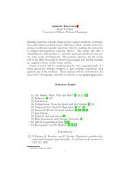
Overview of the Course 

Some Basics: What, Why and How 

Inference and Quantile Treatment Effects 

Nonparametric Quantile Regression 

Quantile Autoregression 

Risk Assessment and Choquet Portfolios 

Course outline, lecture slides, an R FAQ, and even some proposed exercises 

can all be found at: 

http://www.econ.uiuc.edu/~roger/courses/RMetrics. 

A somewhat more extensive set of lecture slides can be found at: 

http://www.econ.uiuc.edu/~roger/courses/LSE. 


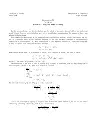
Boxplots of CEO Pay 

annual compensation in millions 

0.1 1 10 100 

* 

+ 

* 

* * 

* * 

* 

+ + + + + + 

* 

+ 

* 

+ 

* 

+ 

● 

● 

● 

● 

0.1 1 10 100 

firm market value in billions 


Motivation 

What the regression curve does is give a grand summary for the 

averages of the distributions corresponding to the set of of x’s. 

We could go further and compute several different regression 

curves corresponding to the various percentage points of the 

distributions and thus get a more complete picture of the set. 


Motivation 






Ordinarily this is not done, and so regression often gives a rather 

incomplete picture. 


Motivation 






Ordinarily this is not done, and so regression often gives a rather 

incomplete picture. Just as the mean gives an incomplete picture 

of a single distribution, so the regression curve gives a 

correspondingly incomplete picture for a set of distributions. 

Mosteller and Tukey (1977) 


Motivation 

Francis Galton in a famous passage defending the “charms of statistics” 

against its many detractors, chided his statistical colleagues 

[who] limited their inquiries to Averages, and do not seem to 

revel in more comprehensive views. Their souls seem as dull to 

the charm of variety as that of a native of one of our flat English 

counties, whose retrospect of Switzerland was that, if the 

mountains could be thrown into its lakes, two nuisances would 

be got rid of at once. Natural Inheritance, 1889 


Univariate Quantiles 

Given a real-valued random variable, X, with distribution function F, we 

define the τth quantile of X as 

Q X (τ) = F −1 

X 

(τ) = inf{x | F(x) τ}. 

This definition follows the usual convention that F is CADLAG, and Q is 

CAGLAD as illustrated in the following pair of pictures. 

F(x) 

0.0 0.2 0.4 0.6 0.8 1.0 

Q(τ) 

0.0 1.0 2.0 3.0 

0.0 1.0 2.0 3.0 

x 

0.0 0.2 0.4 0.6 0.8 1.0 

τ 



Given a real-valued random variable, X, with distribution function F, we 

will define the τth quantile of X as 

Q X (τ) = F −1 

X 

(τ) = inf{x | F(x) τ}. 

This definition follows the usual convention that F is CADLAG, and Q is 

CAGLAD as illustrated in the following pair of pictures. 

F's are CADLAG 

Q's are CAGLAD 

F(x) 

0.0 0.2 0.4 0.6 0.8 1.0 

● 

● 

● 

● 

Q(τ) 

0.0 0.2 0.4 0.6 0.8 1.0 

● 

● 

0.0 0.2 0.4 0.6 0.8 1.0 

x 

0.0 0.2 0.4 0.6 0.8 1.0 

τ 



Viewed from the perspective of densities, the τth quantile splits the area 

under the density into two parts: one with area τ below the τth quantile 

and the other with area 1 − τ above it: 

f(x) 

0.0 0.4 0.8 

τ 

1 − τ 

0.0 0.5 1.0 1.5 2.0 2.5 3.0 

x 


Two Bits Worth of Convex Analysis 

A convex function ρ and its subgradient ψ: 

ρ τ (u) 

τ 

ψ τ (u) 

τ − 1 

τ 

τ − 1 

The subgradient of a convex function f(u) at a point u consists of all the 

possible “tangents.” Sums of convex functions are convex. 


Population Quantiles as Optimizers 

Quantiles solve a simple optimization problem: 

ˆα(τ) = argmin E ρ τ (Y − α) 

Proof: Let ψ τ (u) = ρ ′ τ(u), so differentiating wrt to α: 

0 = 

∫ ∞ 

−∞ 

ψ τ (y − α)dF(y) 

= (τ − 1) 

∫ α 

dF(y) + τ 

−∞ 

∫ ∞ 

α 

dF(y) 

= (τ − 1)F(α) + τ(1 − F(α)) 

implying τ = F(α) and thus ˆα = F −1 (τ). 


● 

● 

● 

● 

● 

● 

● 

● 

● 

● 

● 

● 

● 

● 

● 

● 

● 

● 

● 

● 

● 

● 

● 

● 

● 

● 

● 

● 

● 

● 

● 

● 

● 

● 

● 

● 

● 

● 

● 

● 

● 

● 

Sample Quantiles as Optimizers 

For sample quantiles replace F by ˆF, the empirical distribution function. 

The objective function becomes a polyhedral convex function whose 

derivative is monotone decreasing, in effect the gradient simply counts 

observations above and below and weights the sums by τ and 1 − τ. 

R(x) 

20 30 40 50 60 70 80 

● ●● 

● ● 

●●●● ●● 

● ● 

R'(x) 

−15 −10 −5 0 5 10 15 

−2 0 2 4 

x 

−2 0 2 4 

x 


Conditional Quantiles: The Least Squares Meta-Model 

The unconditional mean solves 

µ = argmin m E(Y − m) 2 





The conditional mean µ(x) = E(Y|X = x) solves 

µ(x) = argmin m E Y|X=x (Y − m(X)) 2 . 







Similarly, the unconditional τth quantile solves 

α τ = argmin a Eρ τ (Y − a) 







Similarly, the unconditional τth quantile solves 

α τ = argmin a Eρ τ (Y − a) 

and the conditional τth quantile solves 

α τ (x) = argmin a E Y|X=x ρ τ (Y − a(X)) 


Computation of Linear Regression Quantiles 

Primal Formulation as a linear program, split the residual vector into 

positive and negative parts and sum with appropriate weights: 

min{τ1 ⊤ u + (1 − τ)1 ⊤ v|y = Xb + u − v, (b, u, v) ∈ |R p × |R 2n 

+ } 

Dual Formulation as a Linear Program 

max{y ′ d|X ⊤ d = (1 − τ)X ⊤ 1, d ∈ [0, 1] n } 

Solutions are characterized by an exact fit to p observations. 

Let h ∈ H index p-element subsets of {1, 2, ..., n} then primal solutions 

take the form: 

ˆβ = ˆβ(h) = X(h) −1 y(h) 


Least Squares from the Quantile Regression Perspective 

Exact fits to p observations: 

ˆβ = ˆβ(h) = X(h) −1 y(h) 

OLS is a weighted average of these ˆβ(h)’s: 

ˆβ OLS = (X ⊤ X) −1 X ⊤ y = ∑ h∈H 

w(h)ˆβ(h), 

w(h) = |X(h)| 2 / ∑ h∈H 

|X(h)| 2 


Least Squares from the Quantile Regression Perspective 

Exact fits to p observations: 

ˆβ = ˆβ(h) = X(h) −1 y(h) 

OLS is a weighted average of these ˆβ(h)’s: 

ˆβ OLS = (X ⊤ X) −1 X ⊤ y = ∑ h∈H 

w(h)ˆβ(h), 

w(h) = |X(h)| 2 / ∑ h∈H 

|X(h)| 2 

The determinants |X(h)| are the (signed) volumes of the parallelipipeds 

formed by the columns of the the matrices X(h). In the simplest bivariate 

case, we have, 

|X(h)| 2 = 

∣ 1 x ∣ 

i ∣∣∣ 

2 

= (x 

1 x j − x i ) 2 

j 

so pairs of observations that are far apart are given more weight. 


Quantile Regression: The Movie 

Bivariate linear model with iid Student t errors 

Conditional quantile functions are parallel in blue 

100 observations indicated in blue 

Fitted quantile regression lines in red. 

Intervals for τ ∈ (0, 1) for which the solution is optimal. 


Quantile Regression in the iid Error Model 

y 

−2 0 2 4 6 8 10 12 

[ 0.069 , 0.096 ] 

● 

● 

● 

● 

● 

● 

● ● ● ● 

● ● ● 

● 

●● 

● 

● 

● 

● 

● 

● ● 

● 

● 

● 

● 

● 

● 

● 

● 

● ●● 

● 

● 

● 

● 

● 

● 

● 

● 

● ● 

● ● 

● 

● 

● ● 

● 

● 

● 

● 

● 

● 

0 2 4 6 8 10 

x 



y 

−2 0 2 4 6 8 10 12 

[ 0.138 , 0.151 ] 

● 

● 

● 

● 

● 

● 

● ● ● ● 

● ● ● 

● 

●● 

● 

● 

● 

● 

● 

● ● 

● 

● 

● 

● 

● 

● 

● 

● 

● ●● 

● 

● 

● 

● 

● 

● 

● 

● 

● ● 

● ● 

● 

● 

● ● 

● 

● 

● 

● 

● 

● 

0 2 4 6 8 10 

x 



y 

−2 0 2 4 6 8 10 12 

[ 0.231 , 0.24 ] 

● 

● 

● 

● 

● 

● 

● ● ● ● 

● ● ● 

● 

●● 

● 

● 

● 

● 

● 

● ● 

● 

● 

● 

● 

● 

● 

● 

● 

● ●● 

● 

● 

● 

● 

● 

● 

● 

● 

● ● 

● ● 

● 

● 

● ● 

● 

● 

● 

● 

● 

● 

0 2 4 6 8 10 

x 



y 

−2 0 2 4 6 8 10 12 

[ 0.3 , 0.3 ] 

● 

● 

● 

● 

● 

● 

● ● ● ● 

● ● ● 

● 

●● 

● 

● 

● 

● 

● 

● ● 

● 

● 

● 

● 

● 

● 

● 

● 

● ●● 

● 

● 

● 

● 

● 

● 

● 

● 

● ● 

● ● 

● 

● 

● ● 

● 

● 

● 

● 

● 

● 

0 2 4 6 8 10 

x 



y 

−2 0 2 4 6 8 10 12 

[ 0.374 , 0.391 ] 

● 

● 

● 

● 

● 

● 

● ● ● ● 

● ● ● 

● 

●● 

● 

● 

● 

● 

● 

● ● 

● 

● 

● 

● 

● 

● 

● 

● 

● ●● 

● 

● 

● 

● 

● 

● 

● 

● 

● ● 

● ● 

● 

● 

● ● 

● 

● 

● 

● 

● 

● 

0 2 4 6 8 10 

x 



y 

−2 0 2 4 6 8 10 12 

[ 0.462 , 0.476 ] 

● 

● 

● 

● 

● 

● 

● ● ● ● 

● ● ● 

● 

●● 

● 

● 

● 

● 

● 

● ● 

● 

● 

● 

● 

● 

● 

● 

● 

● ●● 

● 

● 

● 

● 

● 

● 

● 

● 

● ● 

● ● 

● 

● 

● ● 

● 

● 

● 

● 

● 

● 

0 2 4 6 8 10 

x 



y 

−2 0 2 4 6 8 10 12 

[ 0.549 , 0.551 ] 

● 

● 

● 

● 

● 

● 

● ● ● ● 

● ● ● 

● 

●● 

● 

● 

● 

● 

● 

● ● 

● 

● 

● 

● 

● 

● 

● 

● 

● ●● 

● 

● 

● 

● 

● 

● 

● 

● 

● ● 

● ● 

● 

● 

● ● 

● 

● 

● 

● 

● 

● 

0 2 4 6 8 10 

x 



y 

−2 0 2 4 6 8 10 12 

[ 0.619 , 0.636 ] 

● 

● 

● 

● 

● 

● 

● ● ● ● 

● ● ● 

● 

●● 

● 

● 

● 

● 

● 

● ● 

● 

● 

● 

● 

● 

● 

● 

● 

● ●● 

● 

● 

● 

● 

● 

● 

● 

● 

● ● 

● ● 

● 

● 

● ● 

● 

● 

● 

● 

● 

● 

0 2 4 6 8 10 

x 



y 

−2 0 2 4 6 8 10 12 

[ 0.704 , 0.729 ] 

● 

● 

● 

● 

● 

● 

● ● ● ● 

● ● ● 

● 

●● 

● 

● 

● 

● 

● 

● ● 

● 

● 

● 

● 

● 

● 

● 

● 

● ●● 

● 

● 

● 

● 

● 

● 

● 

● 

● ● 

● ● 

● 

● 

● ● 

● 

● 

● 

● 

● 

● 

0 2 4 6 8 10 

x 



y 

−2 0 2 4 6 8 10 12 

[ 0.768 , 0.798 ] 

● 

● 

● 

● 

● 

● 

● ● ● ● 

● ● ● 

● 

●● 

● 

● 

● 

● 

● 

● ● 

● 

● 

● 

● 

● 

● 

● 

● 

● ●● 

● 

● 

● 

● 

● 

● 

● 

● 

● ● 

● ● 

● 

● 

● ● 

● 

● 

● 

● 

● 

● 

0 2 4 6 8 10 

x 



y 

−2 0 2 4 6 8 10 12 

[ 0.919 , 0.944 ] 

● 

● 

● 

● 

● 

● 

● ● ● ● 

● ● ● 

● 

●● 

● 

● 

● 

● 

● 

● ● 

● 

● 

● 

● 

● 

● 

● 

● 

● ●● 

● 

● 

● 

● 

● 

● 

● 

● 

● ● 

● ● 

● 

● 

● ● 

● 

● 

● 

● 

● 

● 

0 2 4 6 8 10 

x 


Virtual Quantile Regression II 

Bivariate quadratic model with Heteroscedastic χ 2 errors 

Conditional quantile functions drawn in blue 

100 observations indicated in blue 

Fitted quadratic quantile regression lines in red 

Intervals of optimality for τ ∈ (0, 1). 


Quantile Regression in the Heteroscedastic Error Model 

y 

0 20 40 60 80 100 

● 

●● 

● ● 

● 

● ● 

● 

● 

● 

● 

● 

● 

● 

● 

● 

● 

● 

● 

● 

● 

● 

● 

● 

● 

● 

● 

● 

● 

● 

● ● ● ● 

● 

●● 

● 

● 

● ● 

● ● ● 

● ● ● 

●● 

● 

● ● ● 

[ 0.048 , 0.062 ] 

● 

0 2 4 6 8 10 

x 



y 

0 20 40 60 80 100 

● 

●● 

● ● 

● 

● ● 

● 

● 

● 

● 

● 

● 

● 

● 

● 

● 

● 

● 

● 

● 

● 

● 

● 

● 

● 

● 

● 

● 

● 

● ● ● ● 

● 

●● 

● 

● 

● ● 

● ● ● 

● ● ● 

●● 

● 

● ● ● 

[ 0.179 , 0.204 ] 

● 

0 2 4 6 8 10 

x 



y 

0 20 40 60 80 100 

● 

●● 

● ● 

● 

● ● 

● 

● 

● 

● 

● 

● 

● 

● 

● 

● 

● 

● 

● 

● 

● 

● 

● 

● 

● 

● 

● 

● 

● 

● ● ● ● 

● 

●● 

● 

● 

● ● 

● ● ● 

● ● ● 

●● 

● 

● ● ● 

[ 0.261 , 0.261 ] 

● 

0 2 4 6 8 10 

x 



y 

0 20 40 60 80 100 

● 

●● 

● ● 

● 

● ● 

● 

● 

● 

● 

● 

● 

● 

● 

● 

● 

● 

● 

● 

● 

● 

● 

● 

● 

● 

● 

● 

● 

● 

● ● ● ● 

● 

●● 

● 

● 

● ● 

● ● ● 

● ● ● 

●● 

● 

● ● ● 

[ 0.304 , 0.319 ] 

● 

0 2 4 6 8 10 

x 



y 

0 20 40 60 80 100 

● 

●● 

● ● 

● 

● ● 

● 

● 

● 

● 

● 

● 

● 

● 

● 

● 

● 

● 

● 

● 

● 

● 

● 

● 

● 

● 

● 

● 

● 

● ● ● ● 

● 

●● 

● 

● 

● ● 

● ● ● 

● ● ● 

●● 

● 

● ● ● 

[ 0.414 , 0.417 ] 

● 

0 2 4 6 8 10 

x 



y 

0 20 40 60 80 100 

● 

●● 

● ● 

● 

● ● 

● 

● 

● 

● 

● 

● 

● 

● 

● 

● 

● 

● 

● 

● 

● 

● 

● 

● 

● 

● 

● 

● 

● 

● ● ● ● 

● 

●● 

● 

● 

● ● 

● ● ● 

● ● ● 

●● 

● 

● ● ● 

[ 0.499 , 0.507 ] 

● 

0 2 4 6 8 10 

x 



y 

0 20 40 60 80 100 

● 

●● 

● ● 

● 

● ● 

● 

● 

● 

● 

● 

● 

● 

● 

● 

● 

● 

● 

● 

● 

● 

● 

● 

● 

● 

● 

● 

● 

● 

● ● ● ● 

● 

●● 

● 

● 

● ● 

● ● ● 

● ● ● 

●● 

● 

● ● ● 

[ 0.581 , 0.582 ] 

● 

0 2 4 6 8 10 

x 



y 

0 20 40 60 80 100 

● 

●● 

● ● 

● 

● ● 

● 

● 

● 

● 

● 

● 

● 

● 

● 

● 

● 

● 

● 

● 

● 

● 

● 

● 

● 

● 

● 

● 

● 

● ● ● ● 

● 

●● 

● 

● 

● ● 

● ● ● 

● ● ● 

●● 

● 

● ● ● 

[ 0.633 , 0.635 ] 

● 

0 2 4 6 8 10 

x 



y 

0 20 40 60 80 100 

● 

●● 

● ● 

● 

● ● 

● 

● 

● 

● 

● 

● 

● 

● 

● 

● 

● 

● 

● 

● 

● 

● 

● 

● 

● 

● 

● 

● 

● 

● ● ● ● 

● 

●● 

● 

● 

● ● 

● ● ● 

● ● ● 

●● 

● 

● ● ● 

[ 0.685 , 0.685 ] 

● 

0 2 4 6 8 10 

x 



y 

0 20 40 60 80 100 

● 

●● 

● ● 

● 

● ● 

● 

● 

● 

● 

● 

● 

● 

● 

● 

● 

● 

● 

● 

● 

● 

● 

● 

● 

● 

● 

● 

● 

● 

● ● ● ● 

● 

●● 

● 

● 

● ● 

● ● ● 

● ● ● 

●● 

● 

● ● ● 

[ 0.73 , 0.733 ] 

● 

0 2 4 6 8 10 

x 



y 

0 20 40 60 80 100 

● 

●● 

● ● 

● 

● ● 

● 

● 

● 

● 

● 

● 

● 

● 

● 

● 

● 

● 

● 

● 

● 

● 

● 

● 

● 

● 

● 

● 

● 

● ● ● ● 

● 

●● 

● 

● 

● ● 

● ● ● 

● ● ● 

●● 

● 

● ● ● 

[ 0.916 , 0.925 ] 

● 

0 2 4 6 8 10 

x 


Conditional Means vs. Medians 

● 

y 

0 10 20 30 40 

● 

● ● 

● 

mean 

median 

● 

● 

● 

● 

● 

● 

● 

● 

● 

● 

● 

● 

● 

● 

● 

● 

● 

● 

● 

● 

● 

● 

● 

0 2 4 6 8 10 

x 

Minimizing absolute errors for median regression can yield something quite 

different from the least squares fit for mean regression. 


Equivariance of Regression Quantiles 

Scale Equivariance: For any a > 0, ˆβ(τ; ay, X) = aˆβ(τ; y, X) and 

ˆβ(τ; −ay, X) = aˆβ(1 − τ; y, X) 




ˆβ(τ; −ay, X) = aˆβ(1 − τ; y, X) 

Regression Shift: For any γ ∈ |R p ˆβ(τ; y + Xγ, X) = ˆβ(τ; y, X) + γ 




ˆβ(τ; −ay, X) = aˆβ(1 − τ; y, X) 


Reparameterization of Design: For any |A| ≠ 0, 

ˆβ(τ; y, AX) = A −1 ˆβ(τ; yX) 




ˆβ(τ; −ay, X) = aˆβ(1 − τ; y, X) 


Reparameterization of Design: For any |A| ≠ 0, 

ˆβ(τ; y, AX) = A −1 ˆβ(τ; yX) 

Robustness: For any diagonal matrix D with nonnegative elements. 

ˆβ(τ; y, X) = ˆβ(τ, y + Dû, X) 


Equivariance to Monotone Transformations 

For any monotone function h, conditional quantile functions Q Y (τ|x) are 

equivariant in the sense that 

Q h(Y)|X (τ|x) = h(Q Y|X (τ|x)) 

In contrast to conditional mean functions for which, generally, 

E(h(Y)|X) ≠ h(EY|X) 

Examples: 

h(y) = min{0, y}, Powell’s (1985) censored regression estimator. 

h(y) = sgn{y} Rosenblatt’s (1957) perceptron, Manski’s (1975) maximum 

score estimator. estimator. 


Beyond Average Treatment Effects 

Lehmann (1974) proposed the following general model of treatment 

response: 

“Suppose the treatment adds the amount ∆(x) when the 

response of the untreated subject would be x. Then the 

distribution G of the treatment responses is that of the random 

variable X + ∆(X) where X is distributed according to F.” 


Lehmann QTE as a QQ-Plot 

Doksum (1974) defines ∆(x) as the “horizontal distance” between F and 

G at x, i.e. 

F(x) = G(x + ∆(x)). 

Then ∆(x) is uniquely defined as 

∆(x) = G −1 (F(x)) − x. 

This is the essence of the conventional QQ-plot. Changing variables so 

τ = F(x) we have the quantile treatment effect (QTE): 

δ(τ) = ∆(F −1 (τ)) = G −1 (τ) − F −1 (τ). 


Lehmann-Doksum QTE 

P 

0.0 0.2 0.4 0.6 0.8 1.0 

F 

G 

−4 −2 0 2 4 

x 


Lehmann-Doksum QTE 

0.0 0.2 0.4 0.6 0.8 1.0 

P 

Location Shift 

−6 −4 −2 0 2 4 6 

x 

density 

0.0 0.1 0.2 0.3 0.4 

−6 −4 −2 0 2 4 6 

x 

QTE 

0.990 1.000 1.010 

0.0 0.2 0.4 0.6 0.8 1.0 

P 

Scale Shift 

−6 −4 −2 0 2 4 6 

x 

0.0 0.1 0.2 0.3 0.4 

−6 −4 −2 0 2 4 6 

x 

QTE 

−2 −1 0 1 2 

density 

0.0 0.2 0.4 0.6 0.8 1.0 

P 

Location and Scale Shift 

−6 −4 −2 0 2 4 6 

x 

0.0 0.1 0.2 0.3 0.4 

−6 −4 −2 0 2 4 6 

x 

QTE 

−1 0 1 2 3 

density 

0.0 0.2 0.4 0.6 0.8 1.0 

0.0 0.2 0.4 0.6 0.8 1.0 

0.0 0.2 0.4 0.6 0.8 1.0 

u 

u 

u 


An Asymmetric Example 

P 

0.0 0.2 0.4 0.6 0.8 1.0 

density 

0.0 0.1 0.2 0.3 0.4 0.5 0.6 

QTE 

−10 −5 0 5 10 

0 2 4 6 8 10 12 

x 

0 2 4 6 8 10 12 

x 

0.0 0.2 0.4 0.6 0.8 1.0 

u 

Treatment shifts the distribution from right skewed to left skewed making 

the QTE U-shaped. 


QTE via Quantile Regression 

The Lehmann QTE is naturally estimable by 

ˆδ(τ) = Ĝ −1 

n (τ) − ˆF −1 

m (τ) 

where Ĝ n and ˆF m denote the empirical distribution functions of the 

treatment and control observations, Consider the quantile regression model 

Q Yi (τ|D i ) = α(τ) + δ(τ)D i 

where D i denotes the treatment indicator, and Y i = h(T i ), e.g. 

Y i = log T i , which can be estimated by solving, 

min 

n∑ 

ρ τ (y i − α − δD i ) 

i=1 


● 

● 

● 

● 

● 

● ● ● 

● 

● ● ● 

● 

● 

● ● ● ● 

● 

● 

● 

● ● 

● 

● 

● 

● 

● 

● 

● 

● 

● ● ● 

● ● 

● 

● 

● 

● 

● 

● ● 

● 

● 

● 

●● 

● 

● 

● 

● ● 

● 

● 

●● 

● 

● 

● ● 

● ● 

● 

● 

● 

● 

● 

● 

● 

● ● 

● 

● 

● ● 

● ● 

● ● 

● 

● ● 

● 

● 

● ● 

● 

● 

● 

● 

● 

● ● 

● 

● 

● 

● 

● 

● 

● 

● 

● 

● 

● 

● 

● 

●● ● 

●● 

● 

● 

● 

● 

● 

● 

● 

● 

● 

● 

● 

● 

● 

● 

● 

● 

● 

● 

● 

● 

● 

● 

● 

Engel’s Food Expenditure Data 

Food Expenditure 

500 1000 1500 2000 

● ● 

● ● 

● ● 

1000 2000 3000 4000 5000 

Household Income 

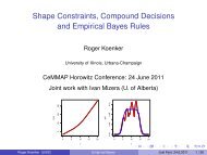
Engel Curves for Food: This figure plots data taken from Engel’s (1857) study of the dependence 

of households’ food expenditure on household income. Seven estimated quantile 

regression lines for τ ∈ {.05, .1, .25, .5, .75, .9, .95} are superimposed on the scatterplot. 

The median τ = .5 fit is indicated by the blue solid line; the least squares estimate of the 

conditional mean function is indicated by the red dashed line. 


● 

● 

● 

● 

● 

● 

● 

● 

● 

● 

● 

● 

● 

● 

● 

● 

● 

● 

● 

● 

● 

● 

● 

● 

● 

● 

● 

●● 

● 

● 

● 

● 

● 

● 

● 

● 

● 

●● 

● 

● 

● 

● 

● 

● 

● 

● 

● 

● 

● 

● 

●● 

● 

● 

● 

● 

● 

● 

● 

● 

● 

● 

● 

● 

● 

● 

● 

● 

● 

● 

● 

● 

● 

● 

● ● 

● 

● 

● 

● 

● 

● 

● 

● 

● 

● 

● 

● 

● 

● 

● 

● 

● 

● 

● 

● ● 

● 

● 

● 

● 

● 

● 

● 

● 

● 

● 

●● 

● 

● 

● 

● 

● 

● 

● 

● 

● 

● 

● 

● 

● 

● 

● 

● 

● 

● 

● 

● 

● 

● 

● 

● 

● 

● 

● 

● 

● 

Engel’s Food Expenditure Data 

Food Expenditure 

300 400 500 600 700 800 

● ● 

400 500 600 700 800 900 1000 

Household Income 

Engel Curves for Food: This figure plots data taken from Engel’s (1857) study of the dependence 

of households’ food expenditure on household income. Seven estimated quantile 

regression lines for τ ∈ {.05, .1, .25, .5, .75, .9, .95} are superimposed on the scatterplot. 

The median τ = .5 fit is indicated by the blue solid line; the least squares estimate of the 

conditional mean function is indicated by the red dashed line. 


A Model of Infant Birthweight 

Reference: Abrevaya (2001), Koenker and Hallock (2001) 

Data: June, 1997, Detailed Natality Data of the US. Live, singleton 

births, with mothers recorded as either black or white, between 18-45, 

and residing in the U.S. Sample size: 198,377. 

Response: Infant Birthweight (in grams) 

Covariates: 

◮ Mother’s Education 

◮ Mother’s Prenatal Care 

◮ Mother’s Smoking 

◮ Mother’s Age 

◮ Mother’s Weight Gain 


Quantile Regression Birthweight Model I 

Intercept 

Boy 

Married 

Black 

2500 3000 3500 4000 

• 

• 

• 

• 

• 

• 

• 

• 

• 

• 

• 

• 

• 

• 

• 

• 

0.0 0.2 0.4 0.6 0.8 1.0 

• 

• 

• 

40 60 80 100 120 140 

• 

• 

• 

• 

• 

• 

• 

• 

• 

• • 

• 

• 

• 

• 

• 

• 

• 

• 

0.0 0.2 0.4 0.6 0.8 1.0 

40 60 80 100 

• 

• 

• 

• 

• 

• • 

• 

• 

• 

• • • 

• • 

• 

• 

0.0 0.2 0.4 0.6 0.8 1.0 

• 

• 

-350 -300 -250 -200 -150 

• 

• 

• 

• 

• 

• • 

• • • 

• 

• 

• • • 

• • 

• • 

0.0 0.2 0.4 0.6 0.8 1.0 

Mother’s Age 

Mother’s Age^2 

High School 

Some College 

30 40 50 60 

• 

• 

• 

• 

• 

• • 

• • 

• 

• 

• • 

• 

• 

• • 

• 

• 

-1.0 -0.8 -0.6 -0.4 

• 

• 

• 

• 

• • 

• 

• • • • 

• • • 

• 

• 

• 

• • 

0 10 20 30 

• 

• • 

• 

• 

• • • 

• 

• 

• 

• 

• 

• 

• 

• 

• 

• 

• 

10 20 30 40 50 

• 

• 

• 

• 

• 

• • • 

• 

• 

• 

• • 

• 

• 

• 

• 

• • 

0.0 0.2 0.4 0.6 0.8 1.0 

0.0 0.2 0.4 0.6 0.8 1.0 

0.0 0.2 0.4 0.6 0.8 1.0 

0.0 0.2 0.4 0.6 0.8 1.0 


Quantile Regression Birthweight Model II 

College 

No Prenatal 

Prenatal Second 

Prenatal Third 

-20 0 20 40 60 80 100 

• 

• 

• 

• • 

• 

• 

• 

• 

• • 

• 

• 

• 

• 

• 

• 

• 

• 

-500 -400 -300 -200 -100 0 

• 

• 

• 

• 

• • 

• 

• • 

• 

• 

• • • 

• • • 

• 

• 

0 20 40 60 

• 

• 

• 

• 

• 

• 

• 

• • • 

• • 

• 

• 

• 

• 

• 

• 

• 

-50 0 50 100 150 

• 

• 

• 

• 

• • • 

• • 

• • • 

• • 

• • • 

• 

• 

0.0 0.2 0.4 0.6 0.8 1.0 

0.0 0.2 0.4 0.6 0.8 1.0 

0.0 0.2 0.4 0.6 0.8 1.0 

0.0 0.2 0.4 0.6 0.8 1.0 

Smoker 

Cigarette’s/Day 

Mother’s Weight Gain 

Mother’s Weight Gain^2 

-200 -180 -160 -140 

• 

• 

• • 

• 

• 

• 

• 

• 

• 

• 

• 

• 

• 

• • 

• • 

• 

-6 -5 -4 -3 -2 

• 

• 

• 

• 

• 

• 

• 

• 

• • • 

• 

• 

• 

• 

• 

• 

• • 

0 10 20 30 40 

• 

• 

• 

• 

• 

• 

• 

• 

• 

• 

• • 

• 

• 

• 

• • 

• 

• 

-0.3 -0.2 -0.1 0.0 0.1 

• 

• 

• 

• 

• 

• • 

• 

• 

• 

• 

• 

• 

• 

• 

• 

• 

• 

• 

0.0 0.2 0.4 0.6 0.8 1.0 

0.0 0.2 0.4 0.6 0.8 1.0 

0.0 0.2 0.4 0.6 0.8 1.0 

0.0 0.2 0.4 0.6 0.8 1.0 


Marginal Effect of Mother’s Age 

Weight Gain Effect 

0.01 0.03 0.05 

● ● 

● 

● 

● 

● 


0.01 0.02 0.03 0.04 

● 

● 

● 

● 

● 

● 

● ● ● ● ● ● ● ● ● ● ● ● ● ● ● ● ● 

● ● ● ● ● ● ● ● ● ● ● ● ● ● ● ● ● 

0.0 0.2 0.4 0.6 0.8 

0.0 0.2 0.4 0.6 0.8 

Quantile 


● 

● 


0.010 0.015 0.020 

● 

● 

● 

● 

● 

● ● ● ● ● ● ● ● ● ● ● ● ● ● ● ● ● 


0.007 0.009 0.011 

● ● 

● 

● 

● 

● ● ● ● 

● ● ● ● ● ● ● ● ● ● ● 

● 0.0 0.2 0.4 0.6 0.8 

0.0 0.2 0.4 0.6 0.8 




Marginal Effect of Mother’s Weight Gain 


0.4 0.5 0.6 0.7 


0.45 0.55 0.65 

20 25 30 35 40 45 

20 25 30 35 40 45 

Mother's Age 

Mother's Age 


0.44 0.48 0.52 0.56 


0.45 0.50 0.55 0.60 

20 25 30 35 40 45 

20 25 30 35 40 45 

Mother's Age 

Mother's Age 


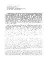
Daily Temperature in Melbourne: AR(1) Scatterplot 

today's max temperature 

10 20 30 40 

10 15 20 25 30 35 40 

yesterday's max temperature 


Daily Temperature in Melbourne: Nonlinear QAR(1) Fit 


10 20 30 40 

10 15 20 25 30 35 40 

yesterday's max temperature 


Conditional Densities of Melbourne Daily Temperature 

Yesterday's Temp 11 



density 

0.05 0.15 

density 

0.00 0.05 0.10 0.15 

density 

0.02 0.06 0.10 

10 12 14 16 18 

12 16 20 24 

15 20 25 30 







density 

0.01 0.03 0.05 0.07 

density 

0.01 0.03 0.05 0.07 

density 

0.01 0.03 0.05 0.07 

15 20 25 30 35 

20 25 30 35 

20 25 30 35 40 





Review 

Least squares methods of estimating conditional mean functions 

were developed for, and 

promote the view that, 

Response = Signal + iid (Gaussian Measurement Error 

In fact the world is rarely this simple. Quantile regression is intended to 

expand the regression window allowing us to see a wider vista.

Quantile Regression: A Gentle Introduction

Create successful ePaper yourself

Delete template?

Save as template?