The Polynom Package
The Polynom Package
The Polynom Package

You also want an ePaper? Increase the reach of your titles
YUMPU automatically turns print PDFs into web optimized ePapers that Google loves.
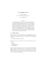
<strong>The</strong> <strong>Polynom</strong> <strong>Package</strong><br />
Copyright 2000–2004<br />
Carsten Heinz < cheinz@gmx.de ><br />
2004/08/12 Version 0.16<br />
Abstract<br />
<strong>The</strong> polynom package implements macros for manipulating polynomials.<br />
For example, it can typeset polynomial long divisions and synthetic divisions<br />
(Horner’s scheme), which can be shown step by step. <strong>The</strong> main test case<br />
and application is the polynomial ring in one variable with rational coefficients.<br />
Please note that this is work in progress. Multivariate polynomials<br />
are currently not supported.<br />
1 Introduction<br />
Donald Arseneau has contributed a lot of packages to the TEX community. In<br />
particular, he posted macros for long division on comp.text.tex, which were also<br />
published in the TUGboat [1] and eventually as longdiv.tex on CTAN. <strong>The</strong><br />
polynom package allows to do the job with polynomials, see figure 1. <strong>The</strong>re you<br />
can also see an example of Horner’s scheme for synthetic division.<br />
X 2 + 2X + 2<br />
X − 1 ) X 3 + X 2 − 1<br />
− X 3 + X 2<br />
2X 2<br />
− 2X 2 + 2X<br />
2X − 1<br />
− 2X + 2<br />
1<br />
\polylongdiv{X^3+X^2-1}{X-1}<br />
1 1 0 − 1<br />
1 1 2 2<br />
1 2 2 1<br />
\polyhornerscheme[x=1]{x^3+x^2-1}<br />
Figure 1: <strong>Polynom</strong>ial long division and synthetic division. <strong>The</strong> commands both<br />
are able to generate partial output, see polydemo.pdf in fullscreen mode.<br />
Figures 2 and 3 show applications of polynomial division. On the one hand the<br />
Euclidean algorithm to determine a greatest common divisor of two polynomials,<br />
1
X 4 − 2X 3 + 2X 2 − 2X + 1 = ( X 3 + X 2 − X − 1 ) · (X<br />
− 3 ) + ( 6X 2 − 4X − 2 )<br />
X 3 + X 2 − X − 1 = ( 6X 2 − 4X − 2 ) · ( 1<br />
6 X + (<br />
18) 5 + 4<br />
9 X − )<br />
4<br />
9<br />
6X 2 − 4X − 2 = ( 4<br />
9 X − ) ( 4<br />
9<br />
· 27<br />
2 X + )<br />
9<br />
2<br />
+ 0<br />
\polylonggcd {(X-1)(X-1)(X^2+1)} {(X-1)(X+1)(X+1)}<br />
Figure 2: Euclidean algorithm with polynomials; the last nonzero remainder is a<br />
greatest common divisor. In the case here, it is uniquely determined up to a scalar<br />
factor, so X − 1 and 4 9 X − 4 9<br />
are both greatest common divisors<br />
\polyfactorize {(X-1)(X-1)(X^2+1)}<br />
(<br />
X 2 + 1 ) ( X − 1 ) 2<br />
\polyfactorize {2X^3+X^2-7X+3}<br />
2 ( X − 1 2) ( X + 1 2 + √ 13<br />
2<br />
) (<br />
X + 1 2 − √ 13<br />
2<br />
\polyfactorize {120X^5-274X^4+225X^3-85X^2+15X-1}<br />
120 ( X − 1 ) ( (<br />
X − 2) 1 X −<br />
1<br />
3<br />
) (<br />
X −<br />
1<br />
4<br />
Figure 3: Factorizations of some polynomials<br />
)<br />
) ( )<br />
X −<br />
1<br />
5<br />
and on the other the factorization of a polynomial with at most two nonrational<br />
zeros. This should suffice for many teaching aids.<br />
2 Hints<br />
As the examples show, the commands get their data through mandatory and<br />
optional arguments. <strong>Polynom</strong>ials are entered as you would type them in math<br />
mode: 1 you may use +, -, *, \cdot, /, \frac, (, ), natural numbers, symbols like<br />
e, \pi, \chi, \lambda, and variables; the power operator ^ with integer exponents<br />
can be used on symbols, variables, and parenthesized expressions. Never use<br />
variables in a nominator, denominator or divisor.<br />
<strong>The</strong> support of symbols is very limited and there is neither support of functions<br />
√<br />
like sin(x) or exp(x), nor of roots or exponents other than integers, for example<br />
π or e x . For teaching purposes this shouldn’t be a major drawback. Particularly<br />
because there is a simple workaround in some cases: the package doesn’t look at<br />
symbols closely, so define a function like e x or ‘composed symbol’ like √ π as a<br />
symbol. Take a look at figure 4 for an example.<br />
Optional arguments are used to specify more general options (and also for the<br />
evaluation point for Horner’s scheme). <strong>The</strong> options are entered in key=value fashion<br />
using the keyval package [3]. <strong>The</strong> available options are listed in the respective<br />
1 <strong>The</strong> scanner is based on the scanner of the calc package [2]. Read its documentation and<br />
the implementation part here if you want to know more.<br />
2
(<br />
e x x 3 − e x x 2 + e x x − e ) x / ( x − 1 ) = e x x 2 + e x<br />
− e x x 3 + e x x 2<br />
e x x − e x<br />
− e x x + e x 0<br />
\newcommand\epowerx{e^x}<br />
\[\polylongdiv{\epowerx x^3-\epowerx x^2+\epowerx x-\epowerx}{x-1}\]<br />
Figure 4: Avoiding problems with e x . Be particularly careful in such cases. You<br />
have to take care of the correct result since the package does the computation.<br />
And by the way, it’s always good to keep an eye on plausibility of the results<br />
sections below.<br />
3 Commands<br />
3.1 \polyset{〈key=value list〉}<br />
Keys and values in optional arguments affect only that particular operation.<br />
\polyset changes the settings for the rest of the current environment or group.<br />
This could be a single figure or the whole document. Almost every key described<br />
in this manual is allowed — just try it and you’ll see. Table 5 lists all keys, which<br />
are not connected to a particular command. An example is<br />
\polyset{vars=XYZ\xi, % make X, Y, Z, and \xi into variables<br />
delims={[}{]}}% nongrowing brackets<br />
Note that is essential to use vars-declared variables only. <strong>The</strong> package can’t guess<br />
your intention and \polylongdiv{\zeta^3+\zeta^2-1}{\zeta-1} would divide<br />
a constant by a constant without the information ζ being a variable.<br />
vars=〈token string〉<br />
delims={〈left〉}{〈right〉}<br />
make each token a variable<br />
define delimiters used for printing<br />
parenthesized expressions<br />
Table 5: General keys. Default for vars is Xx. <strong>The</strong> key delims has in fact an<br />
optional argument which takes invisible versions of the left and right delimiter.<br />
<strong>The</strong> default is delims=[{\left.}{\right.}]{\left(}{\right)}<br />
3
3.2 \polylongdiv[〈key=value list〉]〈polynomial a〉〈polynomial b〉<br />
<strong>The</strong> command prints the polynomial long division of a/b. Applicable keys are<br />
listed in table 6. Of course, vars and delims can be used, too.<br />
stage=〈number〉<br />
style=A|B|C<br />
div=〈token〉<br />
print long division up to stage 〈number〉<br />
(starting with 1)<br />
define output scheme for long division,<br />
refer polydemo.pdf<br />
define division sign for style=C, default<br />
is ÷<br />
Table 6: Keys and values for polynomial long division. style=A requires stage=3×<br />
(#quotient’s summands) + 1 to be carried out fully. <strong>The</strong> other styles B and C need<br />
one more stage if the remainder is nonzero<br />
3.3 \polyhornerscheme[〈key=value list〉]〈polynomial〉<br />
<strong>The</strong> command prints Horner’s scheme for the given polynomial with respect to<br />
the specified evaluation point. Note that the latter one is entered as a key=value<br />
pair in the form 〈variable〉=〈value〉. Table 7 lists other keys and their respective<br />
values.<br />
3.4 \polylonggcd[〈key=value list〉]〈polynomial a〉〈polynomial b〉<br />
<strong>The</strong> command prints equations of the Euclidean algorithm used to determine the<br />
greatest common divisor of the polynomials a and b, refer figure 2.<br />
3.5 \polyfactorize[〈key=value list〉]〈polynomial〉<br />
<strong>The</strong> command prints a factorization of the polynomial as long as all except two<br />
roots are rational, see figure 3.<br />
3.6 Low-level commands<br />
To tell the whole truth, the commands above don’t need the polynomials typed in<br />
verbatim. <strong>The</strong> internal representation of polynomials can be stored as replacement<br />
texts of control sequences and such control sequences can take the role of verbatim<br />
polynomials. This is also the case for 〈a〉 and 〈b〉 in table 8, but each 〈cs ... 〉 must<br />
be a control sequence, in which the result is saved.<br />
<strong>The</strong> command in table 8 can be used for low level calculations, and in particular<br />
to store polynomials for later use with the high-level commands. For example one<br />
could write the following.<br />
4
〈variable〉=〈value〉<br />
<strong>The</strong> definition of the evaluation point is<br />
mandatory!<br />
stage=〈number〉 print Horner’s scheme up to stage<br />
〈number〉 (starting with 1)<br />
tutor=true|false<br />
tutorlimit=〈number〉<br />
tutorstyle=〈font selection〉<br />
resultstyle=〈font selection〉<br />
resultleftrule=true|false<br />
resultrightrule=true|false<br />
resultbottomrule=true|false<br />
showbase=false|<br />
top|middle|bottom<br />
showvar=true|false<br />
showbasesep=true|false<br />
equalcolwidth=true|false<br />
arraycolsep=〈dimension〉<br />
arrayrowsep=〈dimension〉<br />
showmiddlerow=true|false<br />
turn on and off tutorial comments<br />
illustrate the recent 〈number〉 steps<br />
define appearance of tutorial comments<br />
define appearance of the result<br />
control rules left to, right to, and at the<br />
bottom of the result<br />
define whether and in which row the base<br />
(the value) is printed<br />
print or suppress the variable name (additionally<br />
to the base)<br />
print or suppress the vertical rule<br />
use the same width for all columns or use<br />
their individual widths<br />
space between columns<br />
space between rows<br />
print or suppress the middle row<br />
Table 7: Keys and values for Horner’s scheme. Don’t use showmiddlerow=false<br />
with tutor=true.<br />
5
\polyadd\polya {(X^2+X+1)(X-1)-\frac\pi2}{0}% trick<br />
\polymul\polyb {X-1}{1}<br />
% another trick<br />
Let’s see how to divide \polyprint\polya{} by \polyprint\polyb.<br />
\[\polylongdiv\polya\polyb\]<br />
〈cs a+b 〉 ← a + b<br />
〈cs a−b 〉 ← a − b<br />
〈cs ab 〉 ← a · b<br />
〈cs a/b 〉 ← ⌊a/b⌋<br />
\polyremainder ← a mod b<br />
〈cs gcd 〉 ← gcd(a, b)<br />
print polynomial a<br />
\polyadd〈cs a+b 〉〈a〉〈b〉<br />
\polysub〈cs a−b 〉〈a〉〈b〉<br />
\polymul〈cs ab 〉〈a〉〈b〉<br />
\polydiv〈cs a/b 〉〈a〉〈b〉<br />
\polygcd〈cs gcd 〉〈a〉〈b〉<br />
\polyprint〈a〉<br />
Table 8: Low-level user commands<br />
4 Acknowledgments<br />
I wish to thank Ludger Humbert, Karl Heinz Marbaise, and Elke Niedermair for<br />
their tests and error reports.<br />
References<br />
[1] Barbara Beeton and Donald Arseneau.<br />
Long division.<br />
In Jeremy Gibbons’ Hey — it works!, TUGboat 18(2), June 1997, p. 75.<br />
[2] Kresten Krab Thorup, Frank Jensen, and Chris Rowley.<br />
<strong>The</strong> calc package, Infix notation arithmetic in L A TEX, 1998/07/07.<br />
Available from CTAN: macros/latex/required/tools.<br />
[3] David Carlisle.<br />
<strong>The</strong> keyval package, 1999/03/16.<br />
Available from CTAN: macros/latex/required/graphics.<br />
6