(x) is
(x) is
(x) is

You also want an ePaper? Increase the reach of your titles
YUMPU automatically turns print PDFs into web optimized ePapers that Google loves.
Nonlinear Equations<br />
The scient<strong>is</strong>t described what <strong>is</strong>: the engineer creates what never was.<br />
Fall 2010<br />
Theodor von Karman<br />
The father of supersonic flight<br />
1
Problem Description<br />
•Given a non-linear equation f(x)=0, ) find a x*<br />
such that f(x*) = 0. Thus, x* <strong>is</strong> a root of f(x)=0.<br />
•Galo<strong>is</strong> theory in math tells us that only<br />
polynomials l of fdegree ≤ 4 can be solved with<br />
close forms using +, −, ×, ÷ and taking roots.<br />
•General non-linear equations can be solved with<br />
iterative methods.<br />
•Basically, we try to guess the location of a root,<br />
and approximate it iteratively.<br />
•Unfortunately, th<strong>is</strong> process can go wrong, leading<br />
to another root or even diverge.<br />
2
Methods Will Be D<strong>is</strong>cussed<br />
•There are two types of methods, bracketing and<br />
open. The bracketing methods require an<br />
interval that <strong>is</strong> known to contain a root, while<br />
the open method does not.<br />
•Commonly seen bracketing methods include<br />
the b<strong>is</strong>ection method and the regula falsi<br />
method, and the open methods are Newton’s<br />
method, the secant method, and the fixed-point<br />
iteration.<br />
3
B<strong>is</strong>ection Method: 1/6<br />
•Idea: The key <strong>is</strong> the intermediate value theorem.<br />
•If y = f(x) <strong>is</strong> a continuous function on [a,b] and r<br />
<strong>is</strong> between f(a) and f(b), then there <strong>is</strong> a x* such<br />
that r = f(x*).<br />
•Therefore, f if f(a)×f(b)
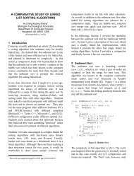
B<strong>is</strong>ection Method: 2/6<br />
•Note that f(a)×f(b) ) ) < 0 guarantees a root in [a,b].<br />
•Compute c = (a+b)/2 and f(c).<br />
•If f(c) = 0, we have found a root.<br />
•Otherw<strong>is</strong>e, either f(a)×f(c) < 0 or f(b)×f(c) < 0 but<br />
not both. Use [a,c] for the former and [c,b] for<br />
the latter until |f(c)| < ε .<br />
1 2<br />
y=f(x) 3<br />
f(a)<br />
4<br />
a<br />
x*<br />
b<br />
f(b)<br />
X<br />
5
B<strong>is</strong>ection Method: 3/6<br />
•Convergence: g Since the first iteration reduces<br />
the interval length to |b-a|/2, the second to |b-a|/2 2 ,<br />
the third to |b-a|/2 3 , etc, after the k-th iteration,<br />
the interval length <strong>is</strong> |b-a|/2 k .<br />
•If ε > 0 <strong>is</strong> a given tolerance value, we have |b-a|/2 k<br />
< ε or |b-a|/ε < 2 k for some k.<br />
•Taking base 2 logarithm, we have the value of k,<br />
the expected number of iterations with accuracy ε:<br />
k = ⎡ ⎢ log 2<br />
b<br />
− a<br />
⎤<br />
ε<br />
⎥<br />
•Convergence g <strong>is</strong> not fast but guaranteed and steady.<br />
6
B<strong>is</strong>ection Method: 4/6<br />
• Algorithm:<br />
• If ABS(b-a) < ε,<br />
then stop.<br />
• Note the red framed<br />
IF statement.<br />
Without th<strong>is</strong>, an<br />
infinite loop can<br />
occur if |b-a| <strong>is</strong> very<br />
small and c can be a<br />
or b due to<br />
rounding.<br />
Fa = f(a)<br />
Fb = f(b) ! Fa*Fb must be < 0<br />
DO<br />
IF (ABS(b-a) < ε) EXIT<br />
c = (a+b)/2<br />
IF (c ==a .OR. c == b) EXIT<br />
Fc = f(c)<br />
IF (Fc == 0) EXIT<br />
IF (Fa*Fc < 0) THEN<br />
b = c<br />
Fb = Fc<br />
ELSE<br />
a = c<br />
Fa = Fc<br />
END IF<br />
END DO<br />
7
B<strong>is</strong>ection Method: 5/6<br />
•However,,<br />
there <strong>is</strong> a catch. ABS(b-a)
B<strong>is</strong>ection Method: 6/6<br />
•The ABS(b-a) < ε may be changed to<br />
ABS(b-a)/MIN(ABS(a),ABS(b)) < ε<br />
•Th<strong>is</strong> test t has a potential ti problem: if the initial<br />
iti bracket contains 0, MIN(ABS(a),ABS(b))<br />
can approach h0 which hwould cause a div<strong>is</strong>ion i i by<br />
zero!<br />
•Nothing <strong>is</strong> perfect!<br />
9
B<strong>is</strong>ection Method Example: 1/3<br />
•Suppose we w<strong>is</strong>h to find the root closest to 6 of<br />
the following equation:<br />
f ( x)<br />
=<br />
sin( i( x<br />
+ cos( x<br />
))<br />
1+<br />
•Plotting the equation f(x) = 0 around x = 6 <strong>is</strong><br />
very helpful.<br />
•You may use gnuplot for plotting. Gnuplot<br />
<strong>is</strong> available free on many platforms such as<br />
Windows, MacOS and Unix/Linux.<br />
x<br />
2<br />
10
B<strong>is</strong>ection Method Example: 2/3<br />
•Function f(x) has a root in [4,6], and f(4) < 0<br />
and f(6) > 0. We may use [4,6] with the<br />
B<strong>is</strong>ection method.<br />
f ( x)<br />
=<br />
sin( x+<br />
cos( x))<br />
2<br />
1+<br />
x<br />
11
B<strong>is</strong>ection Method Example: 3/3<br />
• 19 iterations, x * ≈ 5.5441017… f(x * ) ≈ 0.863277×10 -7 .<br />
[5.5,5.5625]<br />
f ( x<br />
)<br />
=<br />
sin( x + cos( x<br />
))<br />
2<br />
1+ x<br />
[555625] [5.5,5.625]<br />
[5.5,5.75]<br />
[5.5,6]<br />
[4,6]<br />
[5,6]<br />
12
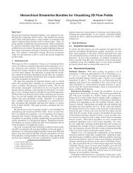
Newton’s Method: 1/13<br />
•Idea:Ifa If a <strong>is</strong> very close to a root of y = f(x) ,the<br />
tangent line though (a, f(a)) intersects the X-ax<strong>is</strong><br />
at a point b that <strong>is</strong> hopefully closer to the root.<br />
•The line through (a, f(a)) with slope f’(a) <strong>is</strong>:<br />
y −<br />
f ( a<br />
) '<br />
= f ( a)<br />
x−<br />
a<br />
y=f(x)<br />
(a,f(a))<br />
a<br />
x*<br />
b<br />
y - f(a) = f ’ (a)×(x-a)<br />
13
Newton’s Method: 2/13<br />
•The line through (a, f(a)) with slope f’(a) <strong>is</strong><br />
y<br />
− f ( a)<br />
x −<br />
a<br />
=<br />
f<br />
'<br />
( a)<br />
•Its intersection point b with the X-ax<strong>is</strong> can be<br />
found by setting y to zero and solving for x:<br />
b<br />
= a<br />
−<br />
f ( a)<br />
'<br />
f ( a)<br />
y=f(x)<br />
(a,f(a))<br />
a<br />
x*<br />
b<br />
14
Newton’s Method: 3/13<br />
•Starting with a x 0 that <strong>is</strong> close to a root x*,<br />
,<br />
Newton’s method uses the following to compute<br />
x 1 , x 2 , … until some x k converges to x*.<br />
.<br />
x<br />
i<br />
+11<br />
= x<br />
i<br />
−<br />
f ( xi<br />
)<br />
'<br />
f ( x )<br />
i<br />
x 0 x 1 x 2 x 3<br />
x*<br />
y=f(x)<br />
15
Newton’s Method: 4/13<br />
•Convergence g 1/2:<br />
•If there <strong>is</strong> a constant ρ, 0 < ρ < 1, such that<br />
x *<br />
− x<br />
lim | |<br />
k + 1<br />
=<br />
ρ<br />
k→∞<br />
*<br />
| xk<br />
− x |<br />
the sequence x 0, x 1, …, <strong>is</strong> said to converge<br />
linearly with ratio (or rate) ρ.<br />
•If ρ <strong>is</strong> zero, the convergence <strong>is</strong> superlinear.<br />
•If x k+1 and x k are close to x*, the above<br />
expression means<br />
|x k+1 – x*| ≈ ρ|x k – x*|<br />
•The error at x k+1 <strong>is</strong> proportional to (i.e.,<br />
linear) and smaller than the error at x k since<br />
ρ < 1.<br />
16
Newton’s Method: 5/13<br />
•Convergence 2/2:<br />
•If there <strong>is</strong> a p > 1 and a C > 0 such that<br />
*<br />
lim | x |<br />
k + 1<br />
− x<br />
= C<br />
k →∞<br />
* p<br />
| x − x |<br />
k<br />
the sequence <strong>is</strong> said to converge with order p.<br />
•If x k+1 and x k are close to x*, , the above<br />
expression yields |x k+1 - x * | ≈ C|x k - x*| p .<br />
•Since |x k - x*| | <strong>is</strong>closeto0andp p >1 1, |x k+1 -x*|<br />
<strong>is</strong> even smaller, and has p more 0 digits.<br />
17
Newton’s Method: 6/13<br />
•The right shows a<br />
possible algorithm that<br />
implements Newton’s<br />
method.<br />
•Newton’smethod<br />
s converges with order 2.<br />
•However, it may not<br />
converge at all, and a<br />
maximum number of<br />
iterations may be needed<br />
to stop early.<br />
x = initial value<br />
Fx = f(x)<br />
Dx = f’(x)<br />
DO<br />
IF (ABS(Fx) < ε) EXIT<br />
New_X = x – Fx/Dx<br />
Fx = f(New_X)<br />
Dx = f’(New_X)<br />
x = New_X<br />
END DO<br />
18
Newton’s Method: 7/13<br />
•Problem 1/6:<br />
• While Newton’s method has a fast<br />
convergence rate, it may not converge at all no<br />
matter how close the initial guess <strong>is</strong>.<br />
verify th<strong>is</strong> fact yourself<br />
y<br />
=<br />
x<br />
1/(2n+<br />
1)<br />
x 3 x 1 x 2<br />
x 4<br />
19
Newton’s Method: 8/13<br />
•Problem 2/6:<br />
• Newton’s method can oscillate.<br />
• If y=f(x)=x x 3 -3x 2 +x+3, then y’=f’(x)=3x 2 -6x+1.<br />
• If the initial value <strong>is</strong> x 0 =1, then we will have x 1<br />
= 2, x 2 = 1, x 3 = 2, …. (see textbook page 78 for<br />
a function plot).<br />
• Note that if x 0 =-1, in 3 iterations the root <strong>is</strong><br />
found at -0.76929265!<br />
• Therefore, carefully choosing an initial guess<br />
<strong>is</strong> important.<br />
20
Newton’s Method: 9/13<br />
•Problem 3/6:<br />
• Newton’s method can oscillate around a<br />
minimal point, eventually causing f’(x) to be<br />
zero.<br />
• In the following, x 1 , x 3 , x 5 , … approach the<br />
minimum i while x 2 , x 4 , …, approach hinfinity.<br />
it<br />
x*<br />
x 1 x 3 x 5 x 2 x 4<br />
21
Newton’s Method: 10/13<br />
•Problem 4/6:<br />
• Since Newton’s method uses x k+1 = x k -<br />
f(x k )/f’(x k ), it requires f’(x k ) ≠ 0.<br />
• As a result, multiple roots can be a problem<br />
because f’(x)=0 at a multiple root.<br />
• Inflection points may also cause problems.<br />
f’(x)=0at = 0 th<strong>is</strong> inflection point<br />
f’(x 2 )=0<br />
f’(x) = 0 at a multiple root<br />
x*<br />
x 2<br />
x 1<br />
22
Newton’s Method: 11/13<br />
•Problem 5/6:<br />
• Newton’s method can converge to a remote<br />
root even though the initial guess <strong>is</strong> close to the<br />
anticipated i t one.<br />
x 2<br />
x*<br />
x 4 x 3<br />
x 1<br />
4<br />
23<br />
But, we get th<strong>is</strong> one<br />
Th<strong>is</strong> <strong>is</strong> what we want!
Newton’s Method: 12/13<br />
•Problem 6/6:<br />
• Even though Newton’s method has a<br />
convergence rate of 2, it can be very slow if the<br />
initial iti guess <strong>is</strong> not right. The following solves<br />
x 10 -1=0. Note that th<strong>is</strong> x * = 1 <strong>is</strong> a multiple root!<br />
slow!<br />
Iteration ti 0 x = 0.5 f(x) = -0.99902343<br />
Iteration 1 x = 51.65 f(x) = 1.3511494E+17<br />
Iteration 2 x = 46.485 f(x) = 4.711166E+16<br />
Iteration 3 x = 41.836502 f(x) = 1.6426823E+16<br />
Iteration 4 x = 37.65285 f(x) = 5.727679E+15<br />
...... Other output ......<br />
Iteration 10 x = 20.01027 f(x) = 1.0292698E+13<br />
...... Other output t ......<br />
Iteration 20 x = 6.9771494 f(x) = 273388500.0<br />
Iteration 30 x = 2.4328012 f(x) = 7261.167<br />
Iteration 40 x = 1.002316 f(x) = 0.02340281<br />
02340281<br />
Iteration 41 x = 1.000024 f(x) = 2.3961067E-4<br />
Iteration 42 x = 1.0 f(x) = 0.0E+0<br />
24
Newton’s Method: 13/13<br />
•A few important notes:<br />
• Newton’s method <strong>is</strong> also referred to as the<br />
Newton-Raphson method.<br />
• Plot the function to find a good initial guess.<br />
• When the computation converges, plug the x*<br />
back to the original equation to make sure it<br />
<strong>is</strong> indeed a root.<br />
• Check for f’(x) = 0.<br />
• The use of a maximum number of iterations<br />
would help prevent infinite loop.<br />
25
Newton’s Method Example: 1/3<br />
•Suppose we w<strong>is</strong>h to find the root closest to 4 of<br />
the following equation:<br />
f ( x ) = sin( e − x<br />
+<br />
cos( x<br />
))<br />
•The following <strong>is</strong> a plot in [0,10]:<br />
f ( x) = sin( e − x + cos( x))<br />
26
Newton’s Method Example: 2/3<br />
•A plot in [4,6] shows that the desired root <strong>is</strong><br />
approximately 4.7, and f(x) <strong>is</strong> monotonically<br />
increasing in [4,6]:<br />
f ( x) = sin( e − x + cos( x))<br />
27
Newton’s Method Example: 3/3<br />
•The following has f(x) and f’(x):<br />
• Initial x 0 = 4.<br />
− x<br />
f ( x) = sin( e + cos( x))<br />
'<br />
−x<br />
−x<br />
f ( x) =− cos( e + cos( x))( e + sin( x))<br />
x f(x) f’(x)<br />
3 iterations<br />
0 4 -0.59344154 0.5943911<br />
x* ≈ 4.703324<br />
1 4.998402 0.2848776 0.9131543<br />
f(x*) ≈ 0.8102506×10 -7 f’(x*) ≈ 0.99089384<br />
2 4.686432 -0.016733877 0.99030494<br />
3 4.703329 0.5750917×10 -5 0.99089395<br />
4 4.703324 0.8102506×10 -7 0.99089384<br />
28
The Secant Method: 1/8<br />
•Idea :Newton’s method requires f’(x). What if<br />
f’(x) <strong>is</strong> difficult to compute or even not available<br />
•Methods that use an approximation g k of f’(x)<br />
are referred to as quasi-Newton methods. Thus,<br />
x k+11 <strong>is</strong> computed (from x k ) as follows:<br />
x<br />
k<br />
+ 1<br />
= xk<br />
−<br />
f ( x )<br />
k<br />
g k<br />
•The secant method offers a simple way for<br />
estimating g k .<br />
29
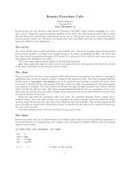
The Secant Method: 2/8<br />
•The secant method uses the slope of the chord<br />
bt between x k-1 and x k as an approximate of ff’( f’(x k ) .<br />
•Therefore, x k+1 <strong>is</strong> the intersection point of th<strong>is</strong><br />
chord and the X-ax<strong>is</strong>. i<br />
•Since the secant method uses two points, it <strong>is</strong><br />
usually referred to as a two-point method.<br />
(x k-1 ,f(x k-1 ))<br />
(x k ,f(x k ))<br />
x k+1<br />
Newton’s method<br />
x* x k x k-1<br />
30
The Secant Method: 3/8<br />
•Since the slope g k <strong>is</strong><br />
g<br />
k<br />
=<br />
f ( x ) − f ( x )<br />
k<br />
x<br />
k<br />
−<br />
x<br />
•Some algebraic manipulations yield the secant<br />
method formula:<br />
k−1<br />
k−1<br />
xk<br />
− xk<br />
1 x −<br />
k+<br />
1<br />
= xk − ×<br />
f ( xk<br />
)<br />
f( x ) − f( x )<br />
k<br />
•It <strong>is</strong> more complex than that of Newton’s method;<br />
but, it may be cheaper than evaluating f’(x k ) .<br />
k−1<br />
31
The Secant Method: 4/8<br />
•Convergence:<br />
• The secant method, in fact all two-point<br />
methods, are superlinear!<br />
• More prec<strong>is</strong>ely, one can show that the<br />
following holds with a 1< p 0<br />
| x *<br />
|<br />
k + 1<br />
− x<br />
lim<br />
k→∞<br />
|<br />
* |<br />
p<br />
x − x<br />
k<br />
• Moreover, p <strong>is</strong> the root of p 2 – p – 1 =0:<br />
=<br />
C<br />
1 = + 5<br />
p =<br />
2<br />
1618 . .....<br />
32
The Secant Method: 5/8<br />
•Algorithm: a = initial value #1<br />
b = initial value #2<br />
•The right <strong>is</strong> the secant Fa = f(a)<br />
method.<br />
Fb = f(b)<br />
DO<br />
•Note that Fb and Fa c = b – Fb*(b-a)/(Fb-Fa)<br />
may be equal, causing Fc = f(c)<br />
IF (ABS(Fc) < ε) EXIT<br />
either overflow or<br />
a = b<br />
div<strong>is</strong>ion by zero!<br />
Fa = Fb<br />
•0/0 <strong>is</strong> also possible!<br />
•Since there are three<br />
subtractions, ti rewrite<br />
the expression to avoid<br />
cancellation if possible.<br />
b = c<br />
Fb = Fc<br />
END DO<br />
33
The Secant Method: 6/8<br />
•The following shows the output of solving f(x) =<br />
x 10 -1 with initial points x 0 =2 and x 1 =1.5.<br />
•It <strong>is</strong> faster than Newton’s method (42 iterations).<br />
a f(a) b f(b)<br />
0 : 2.0 1023.0 1.5 56.66504<br />
1 : 1.5 56.66504 1.4706805 46.33511<br />
2 : 1.4706805 46.33511 1.3391671 17.550165<br />
3 : 1.3391671 17.550165 1.2589835 9.004613<br />
4 : 1.2589835 9.004613 1.1744925 1744925 3.994619<br />
5 : 1.1744925 3.994619 1.1071253 1.7667356<br />
6 : 1.1071253 1.7667356 1.0537024 0.68725025<br />
7 : 1.0537024 0.68725025 1.0196909 0.21530557<br />
8 : 1.0196909 0.21530557 1.0041745 0.04253745<br />
9 : 1.0041745 0.04253745 1.0003542 3.5473108E-3<br />
10 : 1.0003542 3.5473108E-3 1.0000066 6.556511E-5<br />
Converged after 11 iterations x* = 1.0 f(x*) = 0.0E+0<br />
34
The Secant Method: 7/8<br />
•Due to subtractions, cancellation and loss of<br />
significant digits are possible.<br />
•If we start with x 0 =0and x 1 =15 1.5, div<strong>is</strong>ion by<br />
zero can occur! We hit a flat area of the curve.<br />
explain why<br />
Initially:<br />
a = 0.0E+00 f(a) = -1.0 b = 1.5 f(b) = 56.66504<br />
c = 0.026012301 f(c) = -1.0<br />
Iteration 1 :<br />
a = 1.5 f(a) = 56.66504 b = 0.026012301 f(b) = -1.0<br />
c = 0.051573503 f(c) = -1.0<br />
Iteration 2 :<br />
a = 0.026012301 f(a) = -1.0 b = 0.051573503 f(b) = -1.0<br />
Floating exception (Oops!!!)<br />
35
The Secant Method: 8/8<br />
•AA few important notes:<br />
• The secant method evaluates the function<br />
once per iteration.<br />
• Plot the function to find a good initial guess.<br />
• Check if the computed result <strong>is</strong> indeed a root.<br />
• Check for f(x k) – f(x k-1 1) ≈ 0 (i.e., flat area) as<br />
th<strong>is</strong> can cause overflow or div<strong>is</strong>ion by zero.<br />
• The secant method shares essentially the<br />
same pitfalls with Newton’s method.<br />
• The use of a maximum number of iterations<br />
can help prevent infinite loop.<br />
36
Handling Multiple Roots: 1/2<br />
•A polynomial f(x) ) has a root x* of multiplicity ypp<br />
> 1, where p <strong>is</strong> an integer, if f(x) = (x – x*) p g(x)<br />
for some polynomial g(x) and g(x*)≠0.<br />
•Then we have<br />
f(x*) ) = f’(x*) ( ) = f”(x*) ( ) = … f [p-1] (x*) = f [p] (x*) = 0<br />
•For example, f(x) = (x-1)(x-1)(x-2)(x-3) has a<br />
double root (i.e., p = 2) and f(x)=(x-1) ) ( ) 2 g(x) ) and<br />
g(x) = (x-2)(x-3).<br />
•Newton’s method and the secant method,<br />
converge only linearly for multiple roots.<br />
37
Handling Multiple Roots: 2/2<br />
•Two modifications to Newton’s method can still<br />
maintain quadratic convergence.<br />
•If x* <strong>is</strong> a root of multiplicity p, then use the<br />
following instead of the original:<br />
x = +<br />
x − p ×<br />
k<br />
1 k<br />
'<br />
f ( x<br />
)<br />
f<br />
k<br />
( x )<br />
•Or, let g(x) = f(x)/f’(x) and use the following:<br />
x<br />
k<br />
1<br />
x<br />
k<br />
g<br />
( x k<br />
)<br />
g'( x )<br />
k<br />
k<br />
+ = − 38
The Regula Falsi Method: 1/5<br />
•Idea:TheRegula Falsi,akafalse-aka positions,<br />
method <strong>is</strong> a variation of the b<strong>is</strong>ection method.<br />
•The b<strong>is</strong>ection method does not care about the<br />
location of the root. It just cuts the interval at<br />
the mid-point, and, as a result, it <strong>is</strong> slower.<br />
•We may use the intersection point of the X-ax<strong>is</strong><br />
and dthe chord dbetween (a, f(a)) and (b, f(b)) as an<br />
approximation. Hopefully, th<strong>is</strong> would be faster.<br />
39
The Regula Falsi Method: 2/5<br />
•The intersection point c<br />
(a,f(a))<br />
may not be closer to x* than<br />
the mid-point (a+b)/2 <strong>is</strong>.<br />
•The line of (a, f(a)) and (b,<br />
(a+b)/2 x*<br />
f(b)) <strong>is</strong> a c<br />
b<br />
y<br />
− f ( a) f ( b) − f ( a)<br />
=<br />
x−<br />
a b−<br />
a<br />
•Setting y=0 and solving for<br />
x yield c as follows:<br />
c<br />
= a−<br />
b−<br />
a<br />
f ( b) − f ( a)<br />
× f ( a)<br />
= b−<br />
b−<br />
a<br />
f () b − f () a<br />
×<br />
f ( b)<br />
(b,f(b))<br />
40
The Regula Falsi Method: 3/5<br />
•The Regula Falsi<br />
method <strong>is</strong> a variation<br />
of the b<strong>is</strong>ection<br />
method.<br />
•Instead of computing<br />
the mid-point, it<br />
computes the<br />
intersection ti point of<br />
the X-ax<strong>is</strong> and the<br />
chord.<br />
•Otherw<strong>is</strong>e, they are<br />
identical.<br />
Fa = f(a)<br />
Fb = f(b) ! Fa*Fb must be < 0<br />
DO<br />
c = a-Fa*(b-a)/(Fb-Fa)<br />
Fc = f(c)<br />
IF (ABS(Fc) < ε) EXIT<br />
IF (Fa*Fc Fc < 0) THEN<br />
b = c<br />
Fb = Fc<br />
ELSE<br />
a = c<br />
Fa = Fc<br />
END IF<br />
END DO<br />
41
The Regula Falsi Method: 4/5<br />
•The Regula Falsi method can be very slow when<br />
hitting a flat area.<br />
•One of the two end points may be fixed, while<br />
the other end slowly moves the root.<br />
•Near a very flat area f(b) ) – f(a) ) ≈ 0 holds!<br />
x 1 x 2 x 3 x 4 x 5 x 0<br />
x*<br />
42
The Regula Falsi Method: 5/5<br />
•Solving x 10 -1=0 with a = 0 and b = 1.3. Very slow!<br />
a f(a) b f(b) c<br />
1 0.0E+0 -1.0 1.3 12.785842 0.094299644 -1.0<br />
2 0.094299644 -1.0 1.3 12.785842 0.18175896 -0.99999994<br />
3 0.18175896 -0.99999994 1.3 12.785842 0.26287412 -0.99999845<br />
4 0.26287412 -0.99999845 1.3 12.785842 0.33810526 -0.99998044<br />
5 0.33810526 -0.99998044 1.3 12.785842 0.4078781 -0.99987256<br />
10 0.6395442 -0.98855262 1.3 12.785842 0.6869434 -0.97660034<br />
20 0.94343614 -0.44136887 1.3 12.785842 0.95533406 -0.36678296<br />
30 0.99553364 -0.043776333 1.3 12.785842 0.9965725 -0.03375119<br />
40 0.9996887 -3.1086206E-3 1.3 12.785842 0.9997617 -2.3804306E-3<br />
50 0.99997854 -2.1457672E-4 1.3 12.785842 0.99998354 -1.6450882E-4<br />
60 0.99999856 -1.4305115E-5 5 1.3 12.785842 0.9999989 -1.0728836E-5<br />
f(c)<br />
63 0.9999995 -4.7683715E-6<br />
43
Fixed-Point Iteration: 1/19<br />
•Rewrite f(x) = 0 to a new form x = g(x).<br />
• f(x) = sin(x)-cos(x) = 0 becomes sin(x)=cos(x). Hence,<br />
x = sin -1 (cos(x)) ( or x = cos -1 (sin(x)).<br />
( • f(x) = e -x – x 2 = 0 becomes e -x = x 2 . Hence, x = -LOG(x 2 )<br />
or x = SQRT(e -x ).<br />
•The fixed-point iteration starts with an initial value<br />
x 0 and computes x i+1 = g(x i ) until x k+1 ≈ g(x k ) for<br />
some k.<br />
•We are seeking a x* such that x*=g(x*) ) holds.<br />
Th<strong>is</strong> x* <strong>is</strong> a fixed-point of g() since function g()<br />
maps x* to x* itself, and, hence, a root of f(x).<br />
44
Fixed-Point Iteration: 2/19<br />
•The fixed-point iteration x=g(x) can be<br />
considered as computing the intersection point of<br />
the curve y=g(x) and the straight line y = x.<br />
y = x<br />
x* = g(x*)<br />
y = g(x)<br />
45
Fixed-Point Iteration: 3/19<br />
•Let us rewrite x k+1= g(x k )<br />
as y = g(x k ) and x k+1 = y .<br />
•Thus,, y = g(x k ) means<br />
from x k find the y-value of<br />
g(x k ).<br />
•Then, x k+1 = y means use<br />
the y-value to find the<br />
new x-value x k+1 on y = x.<br />
•Repeat th<strong>is</strong> procedure as<br />
shown until, hopefully, it<br />
converges.<br />
Y<br />
y = x<br />
x k+2 = y y = g(x) ( )<br />
x k+1 = y<br />
y = g(x k ) y = g(x k+1 )<br />
X<br />
x k x k+1<br />
46
Fixed-Point Iteration: 4/19<br />
•Newton’s s method uses x k+1 = x k – f(x k )/f’(x k ).Let<br />
g(x) = x – f(x)/f’(x) and Newton’s method<br />
becomes the fixed-point iteration: x k+1 = g(x k ) .<br />
•The fixed-point iteration converges linearly if<br />
|g’(x)| < 1 in the neighborhood of the correct root.<br />
•Observation: if g’(x)∈(0,1) and g’(x)∈(-1,0), the<br />
convergence <strong>is</strong> asymptotic ti and oscillatory,<br />
respectively, and it <strong>is</strong> faster if g’(x) approaches 0.<br />
47
Fixed-Point Iteration: 5/19<br />
•Two convergence cases:<br />
‣ Left g’(x) ∈ (-1,0) and hence oscillatory<br />
‣ Right g’(x) ) ∈ (0,1) and asymptotic tti<br />
g’(x) ) ∈ (-1,0) 10) g’(x) ) ∈ (0,1)<br />
x 1 x 3 x 2<br />
x 1 x 2 x 3<br />
oscillatory<br />
asymptotic<br />
48
Fixed-Point Iteration: 6/19<br />
•Two divergence cases:<br />
‣ Left g’(x) < -1<br />
‣ Right g’(x) )>1<br />
g’(x) < -1<br />
g’(x) > 1<br />
x 3 x 1 x 2 x 4 x 1 x 2 x 3<br />
49
Fixed-Point Iteration: 7/19<br />
•Since f(x) = 0 has to be transformed to a form of<br />
x = g(x) in order to use the fixed-point iteration,<br />
algebraic manipulation <strong>is</strong> necessary.<br />
•Incorrect transformations can yield<br />
roots we don’t want, diverge, or<br />
cause runtime errors.<br />
•As a result, after transformation, ti it<strong>is</strong> very<br />
helpful to plot the curve of y = g(x) and the line y<br />
= x, and dinspect tthe slope g’(x) ) near the desired<br />
d<br />
fixed point to find a good initial guess.<br />
50
Fixed-Point Iteration: 8/19<br />
•Consider f(x) = cos(x) – x 1/2 .<br />
a root in the range of [0,2]<br />
f(x) = cos(x) – x 1/2 51
Fixed-Point Iteration: 9/19<br />
•Setting f(x) to zero yields<br />
cos( x) − x = 0<br />
•Rearranging i terms yields<br />
cos 2 (x) = x.<br />
•We use g(x) = cos 2 (x) for<br />
the fixed-point iteration.<br />
•From curve y = cos 2 (x)<br />
and line y = x, we see only<br />
one root at .64171…..<br />
approximately .<br />
y = cos 2 (x)<br />
y = x<br />
06 0.6 08 0.8<br />
52
Fixed-Point Iteration: 10/19<br />
•Setting g f(x) ) to zero yields<br />
cos( x) − x = 0<br />
•Rearranging terms yields<br />
cos(x) = x 1/2 .<br />
•Taking cos<br />
-1 yields g(x) =<br />
cos -1 (x 1/2 ).<br />
•From y = cos -1 (x 1/2 ) and<br />
line y = x, we see only one<br />
root at 0.64171…..<br />
approximately.<br />
y = cos -1 (x 1/2 )<br />
y = x<br />
06 0.6 08 0.8<br />
53
Fixed-Point Iteration: 11/19<br />
•One may transform f(x) in many ways, each of<br />
which could yield a different root. Some may<br />
diverge or cause runtime errors.<br />
•Again, plotting y = g(x) and y = x and inspecting<br />
the slope g’(x) can help determine the<br />
transformation that can yield the best result.<br />
•For example, the following f(x) ) has two obvious<br />
transformations:<br />
2<br />
f( x) = log( x + 1) − 1+<br />
x<br />
54
Fixed-Point Iteration: 12/19<br />
•Plotting th<strong>is</strong> function f(x) shows that there are<br />
roots in [-0.8, -0.7], [2.0, 3.0] and [70, 80].<br />
55
Fixed-Point Iteration: 13/19<br />
•If we transform f(x) in the following way:<br />
2<br />
log( x<br />
1) 1<br />
+ = +<br />
2 1 x<br />
x<br />
+<br />
1 =<br />
e<br />
+<br />
2 1 x<br />
x e +<br />
= −1<br />
x<br />
1<br />
x e +x<br />
= −1<br />
gx e +x<br />
1<br />
( ) = −1<br />
56
Fixed-Point Iteration: 14/19<br />
•The fixed-point iteration converges to x*=<br />
2.2513…… easily since 0 < g’(x) < 1; but, it <strong>is</strong><br />
difficult to get the other two roots.<br />
Th<strong>is</strong> <strong>is</strong> the asymptotic case<br />
y = x<br />
gx e +x<br />
1<br />
( ) = −1<br />
57
Fixed-Point Iteration: 15/19<br />
•If f(x) <strong>is</strong> transformed in a different way:<br />
2<br />
log( x 1) 1<br />
+ = +<br />
x<br />
(<br />
2<br />
x ) 2<br />
log( + 1) = 1+<br />
x<br />
x<br />
(<br />
2<br />
x ) 2<br />
= log( + 1) −1<br />
( ) 2<br />
x<br />
2<br />
gx ( ) = log( + 1) −1<br />
58
Fixed-Point Iteration: 16/19<br />
Th<strong>is</strong> <strong>is</strong> also the asymptotic case<br />
( ( x<br />
2<br />
)<br />
) 2<br />
gx ( ) = log + 1 −1<br />
If the initial guess <strong>is</strong> larger than x* = 2.2513…<br />
the fixed-point iteration converges to 72.309…<br />
59
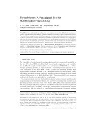
Fixed-Point Iteration: 17/19<br />
Th<strong>is</strong> <strong>is</strong> the oscillatory case<br />
If the initial iti guess <strong>is</strong> less than x* * = 2.2513…<br />
2513<br />
the fixed-point iteration converges to -0.7769…<br />
( ( x<br />
2<br />
)<br />
)<br />
2<br />
g( ( x<br />
) = log + 1 −1<br />
60
Fixed-Point Iteration: 18/19<br />
( ( x<br />
2<br />
)) 2<br />
gx ( ) = log + 1 −1<br />
no way to reach x* = 2.2513…<br />
converge to 72.309…<br />
converge to -0.7769…<br />
61
Fixed-Point Iteration: 19/19<br />
•Conclusion: The fixed-point iteration <strong>is</strong> easy to<br />
use. But, different transformations<br />
may yield different roots and<br />
sometimes may not converge.<br />
Moreover, e some transformations at o s may<br />
lead to runtime errors.<br />
•One may try different transformations to find<br />
the desired root. Only those transformations<br />
that can compute the desired root are considered<br />
correct.<br />
•Use the fixed-point i iteration ti with care.<br />
62
Fixed-Point Iteration Example: 1/9<br />
•Consider the following function f(x):<br />
f ( x) = e − x −sin( x)<br />
•The following plot shows that t f(x) ) = 0h has four<br />
roots in [0,10]. In fact, f(x) = 0 has an infinite<br />
number of roots.<br />
− x<br />
f ( x) = e − sin( x)<br />
=<br />
0<br />
63
Fixed-Point Iteration Example: 2/9<br />
•Since e -x – sin(x) = 0, we have sin(x) = e -x ,andx x =<br />
sin -1 (e -x ). Therefore, we may use g(x) = sin -1 (e -x ).<br />
•We have a problem.<br />
y = g(x) and y=x have only one<br />
intersection point around 0.5.<br />
As a result, only the root in<br />
[0,1] can be found with the<br />
fixed-point iteration.<br />
y = x<br />
−1<br />
−<br />
y = g( x) = sin ( e x )<br />
0.5885…<br />
64
Fixed-Point Iteration Example: 3/9<br />
•Since 0 ≤ e -x ≤ 1, g(x) = sin -1 (e -x ) can be<br />
computed without problems.<br />
•Since e -x decreases monotonically from 1 =<br />
e -0 to 0 as x→∞, sin -1 (e -x ) also decreases<br />
monotonically from π/2 = sin -1 (e -0 )= sin -1 (1)<br />
to 0 as x→∞.<br />
.<br />
•Therefore, g(x) = sin -1 (e -x ) and y = x has<br />
only one intersection ti point, and the fixedpoint<br />
iteration can only find one root of f(x)<br />
= 0.<br />
65
Fixed-Point Iteration Example: 4/9<br />
•Left <strong>is</strong> a plot of g(x) ) in [0,1].<br />
•g’(x) <strong>is</strong> calculated below:<br />
−1<br />
−<br />
gx ( ) = sin ( e x )<br />
−1 1<br />
(sin ( x)) ' =<br />
1−<br />
x<br />
g<br />
( x)<br />
=−<br />
'<br />
− x<br />
e<br />
1−<br />
e<br />
−2x<br />
•Since g’(0.4) = -0.90…, 090 g’(0.5)<br />
= -0.76… , g’(0.6) = -0.66…,<br />
|g’(x)|
Fixed-Point Iteration Example: 5/9<br />
x i<br />
0 0.5<br />
1 0.6516896<br />
2 0.5482148<br />
3 0.616252<br />
4 0.5703949<br />
5 0.6007996<br />
26 iterationsti<br />
x* ≈ 0.58853024<br />
x 0<br />
x 2 x 4<br />
x 5 x 3 x 1<br />
67
Fixed-Point Iteration Example: 6/9<br />
•We may transform e -x –sin(x) = 0 differently.<br />
•Since e -x –sin(x) = 0, we have e -x = sin(x).<br />
•Taking gnatural logarithm yields -x = ln(sin(x))<br />
and hence x = -ln(sin(x)) .<br />
•We may use g(x) = -ln(sin(x)).<br />
•However, th<strong>is</strong> approach has two problems:<br />
• If sin(x) = 0, ln(sin(x)) <strong>is</strong> -∞.<br />
• If sin(x) < 0, ln(sin(x)) <strong>is</strong> not defined.<br />
•Since sin(x) <strong>is</strong> periodic, ln(sin(x)) <strong>is</strong> undefined on<br />
an infinite i number of fintervals (i.e., [π,2π],<br />
[3π,4π], [5π,6π], …). In general, ln(sin(x)) <strong>is</strong><br />
undefined on [(2n-1)π, 2nπ], where n ≥ 1.<br />
68
Fixed-Point Iteration Example: 7/9<br />
y<br />
=<br />
x<br />
A plot shows y = g(x)<br />
and y = x at two<br />
points in (0,π). There<br />
are other roots not in (0,π).<br />
x = 0<br />
g( ( x<br />
) =−ln(sin( ( x<br />
))<br />
x = π<br />
Obviously, the derivative<br />
at th<strong>is</strong> larger root <strong>is</strong> larger<br />
than 1. Hence, the<br />
fixed-point iteration won’t<br />
be able to find it!<br />
Exerc<strong>is</strong>e: Plot g(x) in<br />
[0,20] to see other part.<br />
69
Fixed-Point Iteration Example: 8/9<br />
•Let us examine the smaller root in [0.4,0.6] .<br />
•Since g(x) = -ln(sin(x)), g’(x) <strong>is</strong> (use chain rule):<br />
'<br />
' cos( x<br />
)<br />
g ( x) = ( − ln(sin( x))<br />
= − = −cot( x)<br />
sin( x)<br />
•We have g’(0.4) = -2.36…, g’(0.5) = -1.83…,<br />
g’(0.6) = -1.46….<br />
•Since |g’(x)| > 1 around the root, the fixed-point<br />
iteration diverges and <strong>is</strong> not be able to find the<br />
desired root.<br />
70
Fixed-Point Iteration Example: 9/9<br />
•If we start with x 0 = 0.4, we have x 1 = 0.9431011,<br />
x 2 = 0.2114828, x 3 = 1.561077, x 4 = 0.0000472799,<br />
x 5 = 9.960947<br />
•Since sin(x 5 ) = sin(9.960947) = -0.51084643, g(x 5 )<br />
= g(9.960947) 960947) = ln(sin(-0.51084643)) <strong>is</strong> not welldefined,<br />
and the fixed-point iteration fails.<br />
•Hence, g(x) ( ) = -ln(sin(x)) <strong>is</strong> NOT a correct<br />
transformation.<br />
•You may follow th<strong>is</strong> procedure to do a simple<br />
analys<strong>is</strong> before using the fixed-point iteration.<br />
71
The End<br />
72