A Spectrum Analyzer for the Radio Amateur—Part 2

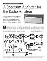
By Wes Hayward, W7ZOI, and Terry White, K7TAU
A Spectrum Analyzer for
the Radio Amateur—Part 2
In Part 1,14 we described the
design and construction of a
simple, yet useful spectrum
analyzer. This installment presents
some applications and methods that
extend the underlying concepts.
Amplifier Gain Evaluation
One use for a spectrum analyzer is amplifier
evaluation. We can illustrate this with a
small amplifier from the test-equipment
drawer—an old module that has been pressed
into service for a variety of experiments. This
circuit, shown in Figure 11, is used for illustration
only and is not presented as an optimum
design. It’s a project that grew from
available parts and may be familiar to some
readers. The circuit uses four identical
2N5179 amplifier stages. A combination of
emitter degeneration and parallel feedback
provides the negative feedback needed to
stabilize gain and impedance. (Ideally, construction
and measurement of a single stage
should precede construction of the complete
amplifier.)
We began the experiment by setting the
signal generator at a known power level,
–20 dBm. (If a good signal generator is unavailable,
you can easily build a suitable
substitute. 15 We used a surplus HP8654A for
most of these experiments.) With the generator
and spectrum analyzer connected to each
other through 50-Ω coax cable, we set the
generator to 14 MHz with 10-dB attenuation
ahead of the analyzer. The amplifier was not
yet connected. We adjusted the analyzer’s IF
GAIN control for a response at the top of
the screen. Using a resolution bandwidth of
300 kHz allows for a fast sweep without distortion.
In our case, the second harmonic was
only 26 dB below the peak response. However,
when we added a 15 MHz low-pass
filter, the second harmonic dropped to
–57 dBc. 16 The third harmonic is well into
the noise. (It is not unusual for a signal generator
to be moderately rich in harmonics.)
Next, we inserted the amplifier between
the signal generator and the analyzer, keeping
the low-pass filter in the generator output.
The on-screen signal went well above
the top as soon as the amplifier was turned
on. Decreasing the signal generator output to
–51 dBm produced the same –20 dBm ana-
14
Notes appear on page 40.
lyzer signal that we saw before the amplifier
was inserted. The gain measured 31 dB. 17 Increasing
the analyzer attenuation by 10 dB
(for a reference level of –10 dBm) and increasing
the generator output to –41 dBm
produced the same gain, but a growing harmonic
output. The second-harmonic response
was now at –43 dBc and a third harmonic
appeared out of the noise at –60 dBc.
We continued the process—moving both
step attenuators produced an amplifier output
of 0 dBm with second and third harmonics
at –28 and –36 dBc, respectively.
The next 10-dB step, however, didn’t work
as well, producing gain compression. With
a drive of –21 dBm, the output was only
+4 dBm, a gain of only 25 dB instead of the
small-signal value of 31 dB.
Amplifier Intermodulation Distortion
Next, we measured intermodulation distortion
(IMD). The setup for these experiments
is shown in Figure 12. Two crystalcontrolled
sources 18 at 14.04 and 14.32 MHz
are combined in a 6 dB hybrid combiner (return-loss
bridge), 19 applied to the 15 MHz
low-pass filter and a step attenuator having
1 dB steps. This composite signal drove the
amplifier, with its output routed to the spectrum
analyzer. For this measurement, we
dropped the resolution bandwidth to 30 kHz.
Here are
some
examples of
procedures
you can use
to become
familiar with
your new
spectrum
analyzer.
(The video filter was turned on and the sweep
rate reduced until the signal amplitude was
stable.) The analyzer’s attenuator, set for a
reference level of –10 dBm at the top of the
screen, was confirmed with a calibration signal
from the signal generator. We adjusted
the IF GAIN to compensate for changes in
analyzer bandwidth and for log-amplifier
drift.
The output of the two-tone generator system
was adjusted to produce a spectrum analyzer
response of –10 dBm per tone. The
IMD responses were readily seen, now 47 dB
below the desired output tones. The output
intercept is given by
IMDR
IP3 out = P out +
2
where P out is the output power of each desired
tone (–10 dBm) and IMDR is the
intermodulation distortion ratio, here 47 dB.
The output intercept for this amplifier measured
+13.5 dBm. This is well in line with
expectations for such a design.
When performing IMD measurements,
it’s a good idea to change the signal level
while noting the resultant performance.
Dropping the drive power by 2 dB should
cause a –2 dB response in the desired
tones, accompanied by a 6 dB drop in distortion-product
tones. The output intercept
September 1998 37

Figure 11—Sample wideband amplifier used to illustrate amplifier measurements.
should remain unchanged.
The IMD in the preceding example was
47 dB below the desired output tones, a value
that we obtained by simply reading it from
the face of the ’scope, possible because we
use a log amplifier that has moderate log fidelity.
If the log amplifier was not as accurate
as it is, we could still get good measurements.
In this example, you would note the
location of the distortion products on the display.
Then, using the step attenuator, decrease
the desired tones until they are at the
noted level. The result would be –47 dBc for
the distortion level, a measurement that depends
solely on the accuracy of the attenuator.
This illustrates the profound utility of a
good step attenuator, an instrument that can
be the cornerstone of an excellent basement
RF laboratory.
During the third-order output-intercept
determination just described, we assumed
that the distortion was a characteristic of the
amplifier under test. This may not be true. It
is important to determine the IMD characteristics
of the spectrum analyzer used for the
measurements before the amplifier measurements
are fully validated. Specifically, for
results to be valid, the input intercept of the
analyzer should be much greater than the
output intercept of the amplifier under test.
The spectrum analyzer input intercept is
easily measured with the same equipment
used to evaluate the amplifier. The two tones
are applied to the analyzer input with no attenuation
present at the analyzer front end.
Then, the input tones are adjusted for a fullscreen
response. In this condition, there
should be no trace of distortion. Although
this is generally an adequate test, it does not
establish a value for the input intercept. To
do that, we must overdrive the analyzer, using
signals that exceed the top of the screen.
The following steps were used to measure
the analyzer input intercept:
• We calibrated the analyzer for a reference
level of –30 dBm with a 30-kHz resolution.
38 September 1998
Figure 12—Equipment setup for evaluation of amplifier intermodulation distortion.
• Confirmed the lack of on-screen distortion
with two tones at the reference level.
• Increased the drive of each tone by
10 dB to provide a pair of –20 dBm tones to
the analyzer. This higher-than-referencelevel
input produced distortion products
66 dB below the reference level, or –96 dBm.
The input signals producing this were each
–20 dBm, so the IMD ratio is (–20) – (–96) =
76 dB. Following the earlier equation, the
input intercept was +18 dBm.
• A 2-dB drive increase produced the expected
6-dB distortion increase. If this had
not occurred, distortion measurements under
overdrive would be suspect. The +18-dBm
value seems to be a good number. This
analyzer generally seems happy with signals
20 dB above the top of the screen, but not
much more.
The intercept for the analyzer with attenuation
in place is the measured value with no
pad plus the attenuation. Hence, with 20 dB
of attenuation, the input intercept will be
+38 dBm, and so forth.
Return-Loss Measurements
The next amplifier characteristic that we
measured was the input impedance match, or
return loss, performed with the setup shown
in Figure 13. With the signal generator set for
a 14-MHz output of about –30 dBm, we set
Figure 13—Test setup for impedancematch
measurements with return-loss
bridge.
the analyzer for full-scale response with the
LOAD port of the return-loss bridge open circuited.
Placing a 50-Ω termination momentarily
on the LOAD port, produced a 38-dB
signal drop. This is a measure of the bridge
directivity. A 38-dB directivity is more than
adequate for casual measurements.
Then, we removed the termination from

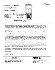
Figure 14—Output of a typical QRP transceiver
kit. The 1-W plus output at 7 MHz is
the dominant signal; all others are
spurious outputs more than 40 dB down,
currently meeting FCC specifications.
Figure 15—Output of a simple homemade
QRP rig. The desired signal is the large
pip at the center of the trace. Two
measurable spurious responses exist, one
to the left and one to the right of the main
signal. The response to the left is 3.5 MHz
feedthrough from the VFO at –64 dBc; the
response to the right of the desired signal
is a second harmonic at –44 dBc.
the bridge and placed it on the amplifier output.
A short length of cable connected the
bridge load port to the amplifier input with
power applied to the amplifier. The result
was a response 20 dB below the top of the
display; 20 dB is the return loss for the amplifier
input, an excellent match for a general-purpose
amplifier. 20 The match improved
slightly when the output load was
removed, an unusual situation.
The next variation measured the output
match for the amplifier. The load was transferred
to the amplifier input and the cable from
the bridge LOAD port was moved to the amplifier
output, producing a reading 15 dB below
the screen top. This match was virtually unchanged
when the input termination was removed.
The weak dependence of both amplifier
return losses is the result of a four-stage
design. A single-stage feedback amplifier will
have port impedances that depend strongly on
the termination at the opposite port.
The –30 dBm drive from the generator
provides an available power of –36 dBm from
the bridge LOAD port. This is low enough
that the amplifier is not over-driven. The
match measurements should be done at a
level low enough that the amplifier remains
linear. In this case, we saw no difference in
the results with drive that was 10 dB higher.
When performing return-loss measurements—and
indeed, most spectrum-analyzer
measurements—it is wise to place at least
10 dB of attenuation ahead of the spectrumanalyzer
mixer. When this attenuation is
switched in, the reference level changes from
the top of the screen to a point down screen a
bit. Return loss is then measured as a decibel
difference with regard to the new reference.
Antenna Measurements
It is interesting to look at some other
impedance values while the return-loss
bridge is attached to the signal generator and
spectrum analyzer. The obvious choice is the
station antenna system, especially if it is
connected through a Transmatch. Playing
with the tuning will readily demonstrate that
the return-loss bridge and sensitive detection
system will allow adjustments to accuracy
unheard of with traditional diode detector
systems. Although such tuning accuracy
is not needed in a normal antenna installation,
it is interesting to see what can be measured
when the need does arise.
Transmitter Evaluation
Another obvious application for a spectrum
analyzer is in transmitter evaluation.
Figure 14 shows the output of a typical QRP
transceiver kit. The 1-W plus output at 7 MHz
is the dominant signal, with all others being
transmitter spurious outputs. All spurs are
more than 40 dB down, which meets current
FCC specifications. On the other hand, significantly
better performance is easily obtained,
especially if the builder has the facilities to
measure them. Figure 15 is a photograph of
a simpler QRP rig with two measurable spurious
responses. One is the 3.5-MHz feedthrough
from the VFO at –64 dBc; the second
is a harmonic at –44 dBc.
The output available from a typical QRP
rig (and certainly higher power rigs) is
enough to damage the spectrum-analyzer
input circuits. Attenuators that we generally
build are capable of handling 0.5 to 1 W
input without damage, while commercial
attenuators are rated at from 0.5 to 2 W input.
The mixers used in this analyzer can be
damaged with as little as 50 to 100 mW signals.
Two methods can be employed to view
the output of a high-power transmitter without
causing damage to the spectrum analyzer.
In one, the transmitter output is run
through a directional coupler with weak coupling
to the sampling port—perhaps –20 to
–30 dB. The majority of the output is dissipated
in a dummy load. The second method
uses a fixed, high-power attenuator. Figure
16 shows an attenuator that will handle
about 20 W while providing 20-dB attenuation.
The design is not symmetrical.
Spectrum Analysis at Higher
Frequencies
Although the 70-MHz spectrum analyzer
is extremely useful, we constantly wish that
it covered higher frequencies. Not only do
we want to experiment on the VHF and UHF
bands, but we need to examine higher-order
harmonics of HF gear. One method we can
use with a regular receiver is a converter,
usually crystal controlled. The same can be
done with a spectrum analyzer, although
crystal control is not needed. We can build a
simple block converter, consisting of nothing
more than a 100 to 200 MHz VCO (just
like that used in the analyzer) and a diode
ring mixer. A Mini-Circuits POS-200 VCO
with a 3 dB pad will directly drive a Mini-
Circuits SBL-1 or TUF-1 mixer to produce a
block converter with a nominal loss of 10 dB.
(One of the spectrum analyzer front-end
boards could be used, with slight modification,
for the block converter.)
This block converter allows analysis of
much of the VHF spectrum. With the converter
VCO set at 100 MHz, frequencies from
100 to 170 MHz are easily studied. The 70 to
100-MHz image is also available—it can also
lead to confusion, as a few minutes with a
signal generator will demonstrate. With the
converter VCO up at 200 MHz, the 200 to
270 MHz spectrum is also available. Clearly,
there is nothing special about the particular
VCO used in the converter. All that is required
to convert other portions of the low UHF
spectrum to the analyzer range is a different
VCO, and perhaps, a higher-frequency mixer.
We will soon build similar block converters
to allow analysis of the 432-MHz area. One
of the popular little UHF frequency counters
is quite useful with these converters. The
block converters should be well shielded
and decoupled from the power supply.
Even without the analyzer, the block converter
is a useful tool. For example, it can be
used with a 10 MHz LC band-pass filter and
an amplifier to directly drive a 50-Ω-terminated
oscilloscope. This can serve as a sensitive
detector for the alignment of a 110-MHz
filter.
As useful as the block downconverter is, it
has image-response problems that can greatly
confuse the results. The preferred way to get
to the higher frequencies is with a spectrum
analyzer—just like the one we have described—but
having higher-frequency oscillators
and front-end filters. If you’re careful,
you can build helical resonator filters for the
500-MHz region, or higher, with sufficiently
narrow selectivity to allow a second conversion
to 10 MHz. A more practical route uses a
third IF. Such a triple-conversion analyzer is
shown in Figure 17, where a 1 to 1.8 GHz
VCO moves signals in the 0 to 800-MHz
spectrum to a 1 GHz IF. This signal is still
easily amplified with available monolithic
amplifiers. Building a 1 GHz filter should not
be too difficult, for a narrow bandwidth is not
required. A bandwidth of 20 or 30 MHz with
a three-resonator filter would be adequate.
The resulting signal is then heterodyned to a
VHF IF (such as 110 MHz) where the remaining
circuitry is now familiar.
Clearly, there are several ways to attack
the project. Recent technology offers some
help in the way of interesting band-pass filter
structures, as well as high-performance,
low-noise VCOs. Time spent with some cata-
September 1998 39

An inside view of a prototype VHF bandpass
filter. See Figure 7.
Figure 16—A 20-W, 20-dB attenuator for transmitter measurements.
Figure 17—Block
diagram for a version of
this analyzer that will
function into the VHF and
low-UHF regions.
logs and a Web browser could be very productive
in this regard. Just as important is the
experience that the lower-frequency analyzer
will provide. Not only is it the tool (perhaps
supplemented with block converters) that is
needed to build a higher-frequency spectrum
analyzer, but it is the vehicle to provide the
confidence needed to tackle such a chore.
Summary
This analyzer has been a useful tool for
over 10 years now. It was a wonderful experience
and fun to build HF and VHF CW
and SSB gear with the “right” test equipment
available. We have built special, narrow-tuning-range
analyzers to examine
transmitter sideband suppression and distortion.
The equipment uses the same concepts
presented.
There are many ways that this instrument
can grow. One builder has already breadboarded
a tracking generator. (Let’s see that
in QST!—Ed.) Many builders will want to
interface the analyzer with a computer instead
of an oscilloscope. A recent QST network
analyzer paper suggests circuits that
may provide such a solution. 21
A recent QST summary of WRC97 22 outlines
new specifications regarding spurious
emissions from amateur transmitters. Gener-
40 September 1998
ally, the casual specifications that we have
enjoyed for many years are being replaced by
new ones that are more stringent—and more
realistic in safeguarding the spectral environment
and reflecting the sound designs that
we all strive to achieve. Equipment such as
the spectrum analyzer described here can
provide the basic tool needed to meet this
new challenge.
Acknowledgments
Many experimenters had a hand in this
project and we owe them our gratitude. Jeff
Damm, WA7MLH, and Kurt Knoblock,
WK7Q, built versions of the analyzer and
have garnered several years of use with them.
Their experiences have been of great value in
our efforts. Barrie Gilbert of Analog Devices
Northwest Labs suggested the AD8307 log
amplifier and provided samples and early
data needed for evaluation measurements.
Many of our colleagues within the Wireless
Communications Division at TriQuint Semiconductor
have helped us with filter measurements:
Thanks go to George Steen and to
Don Knotts, W7HJS. Finally, special thanks
go to our colleague in the receiver group at
TriQuint, Rick Campbell, KK7B, who provided
numerous enlightening discussions
and suggestions regarding the preparation of
the paper and the role of measurements in
amateur experiments.
Notes
14 Wes Hayward, W7ZOI, and Terry White,
K7TAU, “A Spectrum Analyzer for the Radio
Amateur,” Part 1, QST, Aug 1998, pp 35-43.
15 The wide-range oscillator presented in Fig 68,
Chapter 7 of Solid-State Design for the Radio
Amateur (Newington: ARRL, 1997) is still intact
and still often used.
16 The term dBc refers to dB attenuation with
respect to a specific carrier.
17 Formally, this is the transducer gain, or 50-Ω
insertion gain. There are many different parameters
that are called “gain.”
18 The signal sources used are updated versions
of the circuits shown in Fig 66, p 168, in
the Note 15 referent.
19 See page 154, Solid-State Design for the
Radio Amateur.
20 A 20-dB return loss corresponds to a voltage
reflection coefficient of 0.1, or an SWR of
1.222. See Wes Hayward, W7ZOI, Introduction
to RF Design (Newington: ARRL, 1994),
p 120.
21 See, for example, Steven Hageman, “Build
Your Own Network Analyzer,” QST, Jan
1998, pp 39-45; Part 2, Feb 1998, pp 35-39.
22 Larry Price, W4RA, and Paul Rinaldo, W4RI,
“WRC97, An Amateur Radio Perspective,”
QST, Feb 1998, pp 31-34. See also Rick
Campbell, KK7B, “Unwanted Emissions
Comments,” Technical Correspondence,
QST, Jun 1998, pp 61-62.

◊ Please refer to Wes Hayward, W7ZOI, and
Terry White, K7TAU, “A Spectrum Analyzer
for the Radio Amateur—Part 2, QST,
Sep 1998, p 40, Fig 16. The six 2-W input
resistors for the 20-dB pad should be 620 Ω
units, not 820 Ω as originally specified.—
Wes Hayward, W7ZOI (tnx EA2SN)