Derivation of a fundamental diagram for urban traffic flow

More documents

Recommendations

Info

2 The European Physical Journal B density-based approach by Daganzo et al., we will pursue an alternative, utilization-based approach. This is common in queueing theory [39] and transportation planning, where formulas such as the capacity constraint function (1) areused. After discussing elementary relationships for cyclically signalized intersections of urban road networks in Section 2, we will start in Section 3 with the discussion of undersaturated traffic conditions and derive a relationship for the average travel time as a function of the utilization or the number of delayed vehicles. Furthermore, we will determine a formula for the average speed. In Section 4, we will extend the analysis to congested road conditions, where the intersection capacity is exceeded. Afterwards, in Section 5, we will indicate how to deal with oversaturated networks, where the link capacity is insufficient to take up all vehicles that would like to enter a road section. Finally, Section 6 provides a summary and discussion. In particularly, we will address issues regarding the transfer of link-based fundamental diagrams to urban areas. We also try to connect the density-based fundamental diagram of Daganzo et al. with the utilization-based approach developed here. 2 Elementary relationships for cyclically operated intersections Let us study a single intersection with a periodically operated traffic light. We shall have green phases j of duration ΔT j , during which one or several of the traffic streams i are served. β ij shallbe1,iftrafficstreami is served by green phase j, otherwiseβ ij =0.Thesetuptimeafter phase j shall require a time period τ j . It may be imagined to correspond to the time period of the amber light (although in practice, this has to be corrected for reaction times and intersection clearing times). The sum of setup times will be called the “lost service time” T los = ∑ j τ j , (2) while the sum of all green time periods and setup times will be called the “cycle time” T cyc = ∑ j (ΔT j + τ j )=T los + ∑ j ΔT j . (3) The green times are also sometimes expressed as fractions f j ≥ 0 of the cycle time, i.e. ΔT j = f j T cyc (4) with ∑ j f j < 1. After inserting this into equation (3) and rearranging terms, we get T los T cyc ({f j })= 1 − ∑ j f , (5) j i.e. the cycle time is proportional to the lost service time T los . Assuming average inflows A i per lane, the number of vehicles belonging to traffic stream i, which must be served within one cycle time T cyc , amounts to A i T cyc .Inorder to avoid the formation of growing queues (i.e. the onset of congestion), the number of served vehicles per cycle time and lane must reach this value. The number of vehicles of traffic stream i potentially served during the green phases ΔT j is given by ∑ j Q ijβ ij ΔT j per lane, where Q ij denotes the outflow capacity (discharge flow) per lane, when stream i is served by phase j. If we want to have a certain amount of excess capacity to cope with a variability of the inflows, we may demand (1 + δ i )A i T cyc = ∑ j Q ij β ij ΔT j = ∑ j Q ij β ij f j T cyc (6) with δ i > 0. This linear set of equations may be solved for the green time fractions f j . In the following, we will assume the case, where not several traffic streams i are served in parallel by one and the same green phase, but where each phase j serves a single traffic stream i. Then, we may assume β ij =1,ifj = i, andβ ij =0otherwise. Furthermore, Q ij = Q ii = ̂Q i . With this, equation (6) implies f i (u i ,δ i )=(1+δ i ) A i ̂Q i =(1+δ i )u i , (7) where u i = A i (8) ̂Q i is called the utilization of the service or outflow capacity ̂Q i (see Fig. 1). δ i ≥ 0 is a safety factor to cope with variations in the arrival flow (inflow) A i . According to equation (5) wemusthave 0 < 1 − ∑ i f i =1− ∑ i (1 + δ i ) A i ̂Q i . (9) Otherwise, we will have growing vehicle queues from one signal cycle to the next, corresponding to the congested traffic regime. Note that, at time t, thenumberN i (t) of vehicles per lane in the road section reserved for traffic stream i is given by the time integral of the arrival flow A i (t) minus the departure flow γ i (t)O i (t): ∫ t N i (t) = dt ′[ ] A i (t ′ ) − γ i (t ′ )O i (t ′ ) . (10) t 0 Here, the starting time t 0 must be properly chosen to give the correct initial number of vehicles on road section i. During the amber and red time periods, we set the permeability γ i (t) = 0, as there is no outflow, while γ i (t) =1 during green phases. The departure flow O i per lane is given by the service capacity ̂Q i per lane, as long as there
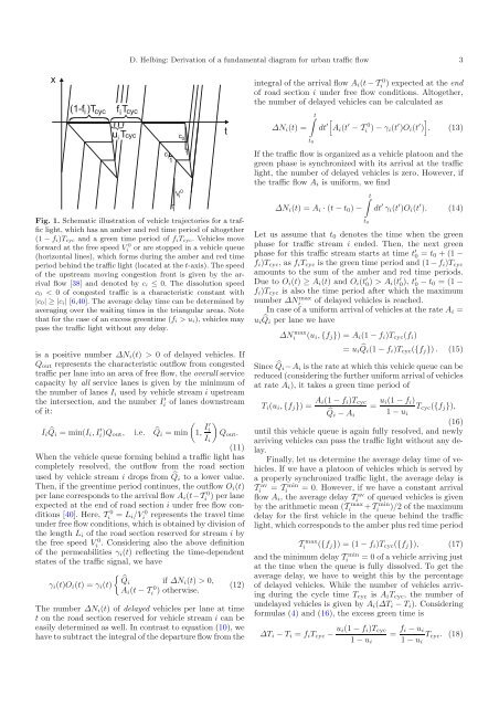
D. Helbing: Derivation of a fundamental diagram for urban traffic flow 3 integral of the arrival flow A i (t −Ti 0 ) expected at the end of road section i under free flow conditions. Altogether, the number of delayed vehicles can be calculated as Fig. 1. Schematic illustration of vehicle trajectories for a traffic light, which has an amber and red time period of altogether (1 − f i)T cyc and a green time period of f iT cyc. Vehicles move forward at the free speed Vi 0 or are stopped in a vehicle queue (horizontal lines), which forms during the amber and red time period behind the traffic light (located at the t-axis). The speed of the upstream moving congestion front is given by the arrival flow [38] and denoted by c i ≤ 0. The dissolution speed c 0 < 0 of congested traffic is a characteristic constant with |c 0|≥|c i| [6,40]. The average delay time can be determined by averaging over the waiting times in the triangular areas. Note that for the case of an excess greentime (f i >u i), vehicles may pass the traffic light without any delay. is a positive number ΔN i (t) > 0 of delayed vehicles. If Q out represents the characteristic outflow from congested traffic per lane into an area of free flow, the overall service capacity by all service lanes is given by the minimum of the number of lanes I i used by vehicle stream i upstream the intersection, and the number I i ′ of lanes downstream of it: ( ) I i ̂Qi =min(I i ,I i ′ )Q out, i.e. ̂Qi =min 1, I′ i Q out . I i (11) When the vehicle queue forming behind a traffic light has completely resolved, the outflow from the road section used by vehicle stream i drops from ̂Q i to a lower value. Then, if the greentime period continues, the outflow O i (t) per lane corresponds to the arrival flow A i (t−Ti 0)perlane expected at the end of road section i under free flow conditions [40]. Here, Ti 0 = L i /Vi 0 represents the travel time under free flow conditions, which is obtained by division of the length L i of the road section reserved for stream i by the free speed Vi 0 . Considering also the above definition of the permeabilities γ i (t) reflecting the time-dependent states of the traffic signal, we have { ̂Qi if ΔN γ i (t)O i (t) =γ i (t) i (t) > 0, A i (t −Ti 0)otherwise. (12) The number ΔN i (t) ofdelayed vehicles per lane at time t on the road section reserved for vehicle stream i can be easily determined as well. In contrast to equation (10), we have to subtract the integral of the departure flow from the ΔN i (t) = ∫ t dt ′[ ] A i (t ′ −Ti 0 ) − γ i(t ′ )O i (t ′ ) . (13) t 0 If the traffic flow is organized as a vehicle platoon and the green phase is synchronized with its arrival at the traffic light, the number of delayed vehicles is zero. However, if the traffic flow A i is uniform, we find ∫ t ΔN i (t) =A i · (t − t 0 ) − t 0 dt ′ γ i (t ′ )O i (t ′ ). (14) Let us assume that t 0 denotes the time when the green phase for traffic stream i ended. Then, the next green phase for this traffic stream starts at time t ′ 0 = t 0 +(1− f i )T cyc ,asf i T cyc is the green time period and (1 − f i )T cyc amounts to the sum of the amber and red time periods. Due to O i (t) ≥ A i (t) andO i (t ′ 0) >A i (t ′ 0), t ′ 0 − t 0 =(1− f i )T cyc is also the time period after which the maximum number ΔNi max of delayed vehicles is reached. In case of a uniform arrival of vehicles at the rate A i = u i ̂Qi per lane we have ΔNi max (u i , {f j })=A i (1 − f i )T cyc (f i ) = u i ̂Qi (1 − f i )T cyc ({f j }) . (15) Since ̂Q i −A i is the rate at which this vehicle queue can be reduced (considering the further uniform arrival of vehicles at rate A i ), it takes a green time period of T i (u i , {f j })= A i(1 − f i )T cyc = u i(1 − f i ) T cyc ({f j }), ̂Q i − A i 1 − u i (16) until this vehicle queue is again fully resolved, and newly arriving vehicles can pass the traffic light without any delay. Finally, let us determine the average delay time of vehicles. If we have a platoon of vehicles which is served by a properly synchronized traffic light, the average delay is Ti av = Ti min = 0. However, if we have a constant arrival flow A i , the average delay T av of queued vehicles is given i by the arithmetic mean (Ti max +Ti min )/2 ofthemaximum delay for the first vehicle in the queue behind the traffic light, which corresponds to the amber plus red time period T max i ({f j })=(1− f i )T cyc ({f j }), (17) and the minimum delay Ti min = 0 of a vehicle arriving just at the time when the queue is fully dissolved. To get the average delay, we have to weight this by the percentage of delayed vehicles. While the number of vehicles arriving during the cycle time T cyc is A i T cyc ,thenumberof undelayed vehicles is given by A i (ΔT i − T i ). Considering formulas (4) and(16), the excess green time is ΔT i − T i = f i T cyc − u i(1 − f i )T cyc 1 − u i = f i − u i 1 − u i T cyc . (18)
Page 1: Eur. Phys. J. B (2009) DOI: 10.1140
Page 5 and 6: D. Helbing: Derivation of a fundame
Page 13: D. Helbing: Derivation of a fundame

Derivation of a fundamental diagram for urban traffic flow

You also want an ePaper? Increase the reach of your titles

Delete template?

Save as template?