Derivation of a fundamental diagram for urban traffic flow

More documents

Recommendations

Info

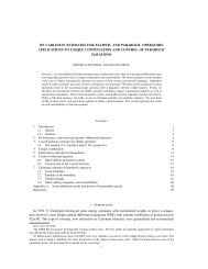
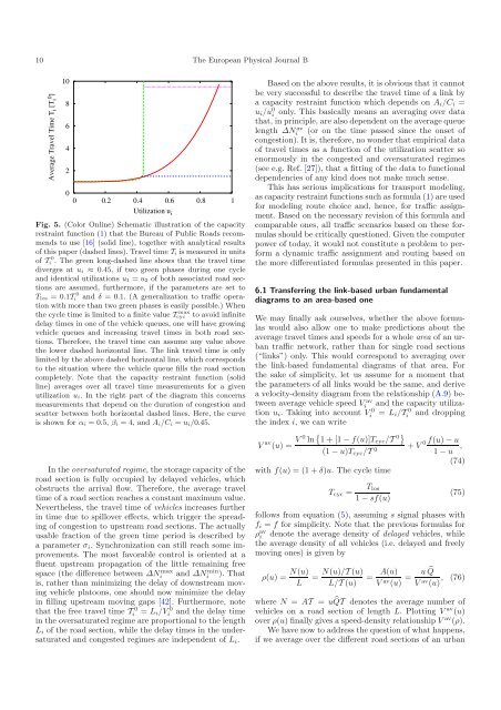
10 The European Physical Journal B Average Travel Time T i [T i 0 ] 10 8 6 4 2 0 0 0.2 0.4 0.6 0.8 1 Utilization u i Fig. 5. (Color Online) Schematic illustration of the capacity restraint function (1) that the Bureau of Public Roads recommends to use [16] (solid line), together with analytical results of this paper (dashed lines). Travel time T i is measured in units of Ti 0 . The green long-dashed line shows that the travel time diverges at u i ≈ 0.45, if two green phases during one cycle and identical utilizations u 1 = u 2 of both associated road sections are assumed, furthermore, if the parameters are set to T los =0.1Ti 0 and δ =0.1. (A generalization to traffic operation with more than two green phases is easily possible.) When the cycle time is limited to a finite value Tcyc max to avoid infinite delay times in one of the vehicle queues, one will have growing vehicle queues and increasing travel times in both road sections. Therefore, the travel time can assume any value above the lower dashed horizontal line. The link travel time is only limited by the above dashed horizontal line, which corresponds to the situation where the vehicle queue fills the road section completely. Note that the capacity restraint function (solid line) averages over all travel time measurements for a given utilization u i. In the right part of the diagram this concerns measurements that depend on the duration of congestion and scatter between both horizontal dashed lines. Here, the curve is shown for α i =0.5, β i =4,andA i/C i = u i/0.45. In the oversaturated regime, the storage capacity of the road section is fully occupied by delayed vehicles, which obstructs the arrival flow. Therefore, the average travel time of a road section reaches a constant maximum value. Nevertheless, the travel time of vehicles increases further in time due to spillover effects, which trigger the spreading of congestion to upstream road sections. The actually usable fraction of the green time period is described by a parameter σ i . Synchronization can still reach some improvements. The most favorable control is oriented at a fluent upstream propagation of the little remaining free space (the difference between ΔNi max and ΔNi min ). That is, rather than minimizing the delay of downstream moving vehicle platoons, one should now minimize the delay in filling upstream moving gaps [42]. Furthermore, note that the free travel time Ti 0 = L i /Vi 0 and the delay time in the oversaturated regime are proportional to the length L i of the road section, while the delay times in the undersaturated and congested regimes are independent of L i . Based on the above results, it is obvious that it cannot be very successful to describe the travel time of a link by a capacity restraint function which depends on A i /C i = u i /u 0 i only. This basically means an averaging over data that, in principle, are also dependent on the average queue length ΔNi av (or on the time passed since the onset of congestion). It is, therefore, no wonder that empirical data of travel times as a function of the utilization scatter so enormously in the congested and oversaturated regimes (see e.g. Ref. [27]), that a fitting of the data to functional dependencies of any kind does not make much sense. This has serious implications for transport modeling, as capacity restraint functions such as formula (1)areused for modeling route choice and, hence, for traffic assignment. Based on the necessary revision of this formula and comparable ones, all traffic scenarios based on these formulas should be critically questioned. Given the computer power of today, it would not constitute a problem to perform a dynamic traffic assignment and routing based on the more differentiated formulas presented in this paper. 6.1 Transferring the link-based urban fundamental diagrams to an area-based one We may finally ask ourselves, whether the above formulas would also allow one to make predictions about the average travel times and speeds for a whole area of an urban traffic network, rather than for single road sections (“links”) only. This would correspond to averaging over the link-based fundamental diagrams of that area. For the sake of simplicity, let us assume for a moment that the parameters of all links would be the same, and derive a velocity-density diagram from the relationship (A.9) between average vehicle speed Vi av and the capacity utilization u i . Taking into account Vi 0 = L i /Ti 0 and dropping the index i, wecanwrite V av (u) = V 0 ln { 1+[1− f(u)]T cyc /T 0} (1 − u)T cyc /T 0 + V 0 f(u) − u 1 − u , (74) with f(u) =(1+δ)u. The cycle time T cyc = T los 1 − sf(u) (75) follows from equation (5), assuming s signal phases with f i = f for simplicity. Note that the previous formulas for ρ av i denote the average density of delayed vehicles, while the average density of all vehicles (i.e. delayed and freely moving ones) is given by ρ(u) = N(u) L N(u)/T (u) = = A(u) L/T (u) V av (u) = u ̂Q V av (u) , (76) where N = AT = u ̂QT denotes the average number of vehicles on a road section of length L. Plotting V av (u) over ρ(u) finally gives a speed-density relationship V av (ρ). We have now to address the question of what happens, if we average over the different road sections of an urban
D. Helbing: Derivation of a fundamental diagram for urban traffic flow 11 area. Considering the heterogeneity of the link lengths L i , efficiencies ɛ i , utilizations u i , and densities ρ av i , one could think that the spread in the data would be enormous. However, a considerable amount of smoothing results from the fact that in- and outflows of links within the studied urban area cancel out each other, and it does not matter whether a vehicle is delayed in a particular link, or in the previous or subsequent one. Therefore, the resulting fundamental diagrams for urban areas are surprisingly smooth [29,30]. The details of the curves, however, are expected to depend not only on the average density, but also on the density distribution, the signal operation schemes, and potentially other factors as well. When averaging over different links, we have to study the effects of the averaging procedure on the density and the speed. The density just averages linearly: thanks to Little’s law [39], the formula (76) can also be applied to an urban area, as long as the average number of vehicles in it is stationary. However, as the link-based fundamental diagram between the flow Q(ρ) =ρV av (ρ) andthedensity ρ is convex, evaluating the flow at some average density overestimates the average flow 2 . This also implies that, when the relationship V av (ρ) is transferred from single links to urban areas, the average speed is overestimated for a given density, as reference [31] hasshown. Despite this expected deviation in heterogeneous and inhomogeneously used road networks, and despite the many other simplifications, the curve V av (ρ) fitsempirical data of the speed-density relation in an urban area quite well. Figure 6 displays empirical data obtained for the center of Yokohama [29] together with a fit of the theoretical speed-density relationship V av (ρ), where only the three parameters V 0 , δ, andV ∗ = L/T los were adjusted. Surprisingly, the effects of network interactions could be sufficiently well represented by a single parameter δ,which relates to the efficiency ɛ of road sections according to equation (32). This approximation seems to work in situations close enough to a statistical equilibrium (when the number of vehicles in the urban area does not change too quickly). In contrast, for an understanding of the spreading dynamics of congestion patterns, we expect that one must study the interaction between the flow dynamics and the network structure. This difficult subject goes beyond the scope of this paper and beyond what is doable at the moment, but it will be interesting to address it in the future. 2 When averaging over speed values, they have to be weighted by the number of vehicles concerned, i.e. by the density. This comes down to determining an arithmetic average of the flow values and dividing the result by the arithmetic average of the related densities. Hence, an overestimation of the average flow also implies an overestimation of the average velocity. However, considering the curvature of Q(ρ) and knowing the variability of the density ρ allows one to estimate correction terms. 3 This corresponds to 10% extra green time, an average distance between successive traffic lights of roughly 100 m (depending on T los ), and an average of 3 traffic phases (which appears plausible, considering that there are many one-way roads, Speed (km/h) 35 30 25 20 15 10 5 0 0 0.02 0.04 0.06 0.08 0.1 Density (1/m) Fig. 6. (Color online) Fundamental velocity-density relationship for a central area of Yokohama. Small circles correspond to empirical data by Kuwahara as evaluated by Daganzo and Geroliminis [31]. The fit curve corresponds to the theoretically derived equations (74) to(76), where the outflow (discharge flow) ̂Q = 1800 veh./h/lane and the free speed V 0 = 50 km/h have been fixed. The only fit parameters were δ =0.1, T los /T 0 =1.4, and s =3 3 . The author thanks for an inspiring presentation by Carlos Daganzo, for useful comments by Stefan Lämmer, and intresting discussions with Nikolas Geroliminis, who was also kind enough to provide the empirical data from the center of Yokohama displayed in Figure 6, see Figure 7 in reference [29]. He extracted these from original data of GPS-equipped taxis by Prof. Masao Kuwahara from the University of Tokyo. The fit of the theoretically predicted relationship to the empirical data was carried out by Anders Johansson. Furthermore, the author is grateful for partial support by the Daimler- Benz Foundation Project 25-01.1/07 on BioLogistics, the VW Foundation Project I/82 697, the NAP project KCKHA005 “Complex Self-Organizing Networks of Interacting Machines: Principles of Design, Control, and Functional Optimization”, and the ETH Competence Center ‘Coping with Crises in Complex Socio-Economic Systems’ (CCSS) through ETH Research Grant CH1-01-08-2. Appendix A: Determination of average travel times and velocities Let f(x) be a function and w(x) a weight function. Then, the average of the function between x = x 0 and x = x 1 is which need less than 4 phases in one cycle time). Consequently, all parameters are quite reasonable (see also Ref. [31]). Note that effects of oversaturation did not have to be considered in Figure 6. This is, in fact, consistent with pictures from Google Earth.
Page 1 and 2: Eur. Phys. J. B (2009) DOI: 10.1140
Page 3 and 4: D. Helbing: Derivation of a fundame
Page 9: D. Helbing: Derivation of a fundame
Page 13: D. Helbing: Derivation of a fundame

Derivation of a fundamental diagram for urban traffic flow

Create successful ePaper yourself

Delete template?

Save as template?