Derivation of a fundamental diagram for urban traffic flow

Eur. Phys. J. B (2009)
DOI: 10.1140/epjb/e2009-00093-7
Regular Article
THE EUROPEAN
PHYSICAL JOURNAL B
Derivation of a fundamental diagram for urban traffic flow
D. Helbing a
ETH Zurich, UNO D11, Universitätstr. 41, 8092 Zurich, Switzerland
Received 11 July 2008 / Received in final form 22 December 2008
Published online 14 March 2009 – c○ EDP Sciences, Società Italiana di Fisica, Springer-Verlag 2009
Abstract. Despite the importance of urban traffic flows, there are only a few theoretical approaches to
determine fundamental relationships between macroscopic traffic variables such as the traffic density, the
utilization, the average velocity, and the travel time. In the past, empirical measurements have primarily
been described by fit curves. Here, we derive expected fundamental relationships from a model of traffic
flows at intersections, which suggest that the recently measured fundamental diagrams for urban flows
can be systematically understood. In particular, this allows one to derive the average travel time and the
average vehicle speed as a function of the utilization and/or the average number of delayed vehicles.
PACS. 89.40.Bb Land transportation – 47.10.ab Conservation laws and constitutive relations – 51.10.+y
Kinetic and transport theory of gases
1 Introduction
The study of urban traffic flows has a long history (see
Ref. [1] for an overview). For more than a decade now,
physicists have contributed various interesting models,
ranging from cellular automata [2–4] to fluid-dynamic approaches
[5,6]. Complementary, one should mention, for
example, reference [7,8] as representatives of publications
by traffic engineers, and also continuous microscopic flow
models used in commercial software tools such as VISSIM.
One research area in traffic physics is the transition
from free to congested traffic in urban road networks
[9,10], which started off with the paper by Biham
et al. [11]. Interestingly enough, the spreading of congestion
seems to share some features with cascading failures
[12].
In the following, we will focus on the study of fundamental
relationships between flow, utilization, and density
on the one hand and the average velocity or travel time
on the other hand. Such relationships were already studied
in the 60ies [13–23], but this work primarily took a
phenomenological approach. Moreover, the recorded data
in the regime of congested road networks scattered enormously.
Thus, it was hard to fit a curve. Consequently,
many different relationships were proposed. The probably
most wide-spread formula is the one published by the Bureau
of Public Roads [16]. Accordingly, the travel time T i
of an urban road section i with capacity C i would follow
the capacity constraint function
a
T i = T 0
i
[
e-mail: dhelbing@ethz.ch
1+α i
(
Ai
C i
) βi
]
. (1)
(see Fig. 5). Here, A i is the arrival flow in that road section
and Ti
0 the travel time for light traffic conditions,
while α i ≈ 0.5 andβ i ≈ 4 are fit parameters. It is obvious
that this formula does not diverge when the capacity C i is
reached, as one may expect. This is just one of the many
theoretical inconsistencies of the proposed phenomenological
formulas. It is no wonder that the subject of fundamental
diagrams for urban traffic has recently been taken
up again [24–31].
The first measurement of an urban fundamental diagram
was presented by Godfrey [32]. Ten years later, even
Robert Herman and nobel prize laureate Ilya Prigogine
addressed traffic flow in cities [33,34]. They tried to derive
fundamental relationships via a statistical physics approach,
which however still contained phenomenological
elements. Their “two-fluid approach” considered moving
and standing traffic and the mutual interdependencies between
them.
Recently, the issue of urban gridlock was reanimated
by Carlos Daganzo [28]. Together with Geroliminis, he
presented convincing evidence for a fundamental diagram
of urban traffic flow [29,30]. Before, fundamental diagrams
were mainly used for the study of freeway systems [36].
There, they were very useful to understand capacity effects
[1], different traffic states [37], and the traffic dynamics,
in particularly the propagation of shock fronts [38]. It
is, therefore, not surprising that people are eager to find
fundamental relationships for urban traffic as well.
The most recent progress is an approximation of the
urban fundamental diagram by Daganzo and Geroliminis,
which is based on cutting away parts of the flow-density
plane [31]. It appears possible to construct a relationship
with kinematic wave theory [35]. In contrast to the

2 The European Physical Journal B
density-based approach by Daganzo et al., we will pursue
an alternative, utilization-based approach. This is common
in queueing theory [39] and transportation planning,
where formulas such as the capacity constraint function
(1) areused.
After discussing elementary relationships for cyclically
signalized intersections of urban road networks in Section
2, we will start in Section 3 with the discussion of
undersaturated traffic conditions and derive a relationship
for the average travel time as a function of the utilization
or the number of delayed vehicles. Furthermore, we will
determine a formula for the average speed. In Section 4,
we will extend the analysis to congested road conditions,
where the intersection capacity is exceeded. Afterwards,
in Section 5, we will indicate how to deal with oversaturated
networks, where the link capacity is insufficient to
take up all vehicles that would like to enter a road section.
Finally, Section 6 provides a summary and discussion.
In particularly, we will address issues regarding the
transfer of link-based fundamental diagrams to urban areas.
We also try to connect the density-based fundamental
diagram of Daganzo et al. with the utilization-based approach
developed here.
2 Elementary relationships for cyclically
operated intersections
Let us study a single intersection with a periodically operated
traffic light. We shall have green phases j of duration
ΔT j , during which one or several of the traffic streams i
are served. β ij shallbe1,iftrafficstreami is served by
green phase j, otherwiseβ ij =0.Thesetuptimeafter
phase j shall require a time period τ j . It may be imagined
to correspond to the time period of the amber light (although
in practice, this has to be corrected for reaction
times and intersection clearing times). The sum of setup
times will be called the “lost service time”
T los = ∑ j
τ j , (2)
while the sum of all green time periods and setup times
will be called the “cycle time”
T cyc = ∑ j
(ΔT j + τ j )=T los + ∑ j
ΔT j . (3)
The green times are also sometimes expressed as fractions
f j ≥ 0 of the cycle time, i.e.
ΔT j = f j T cyc (4)
with ∑ j f j < 1. After inserting this into equation (3) and
rearranging terms, we get
T los
T cyc ({f j })=
1 − ∑ j f , (5)
j
i.e. the cycle time is proportional to the lost service time
T los .
Assuming average inflows A i per lane, the number of
vehicles belonging to traffic stream i, which must be served
within one cycle time T cyc , amounts to A i T cyc .Inorder
to avoid the formation of growing queues (i.e. the onset of
congestion), the number of served vehicles per cycle time
and lane must reach this value. The number of vehicles of
traffic stream i potentially served during the green phases
ΔT j is given by ∑ j Q ijβ ij ΔT j per lane, where Q ij denotes
the outflow capacity (discharge flow) per lane, when
stream i is served by phase j. If we want to have a certain
amount of excess capacity to cope with a variability of the
inflows, we may demand
(1 + δ i )A i T cyc = ∑ j
Q ij β ij ΔT j = ∑ j
Q ij β ij f j T cyc (6)
with δ i > 0. This linear set of equations may be solved
for the green time fractions f j . In the following, we will
assume the case, where not several traffic streams i are
served in parallel by one and the same green phase, but
where each phase j serves a single traffic stream i. Then,
we may assume β ij =1,ifj = i, andβ ij =0otherwise.
Furthermore, Q ij = Q ii = ̂Q i . With this, equation (6)
implies
f i (u i ,δ i )=(1+δ i ) A i
̂Q i
=(1+δ i )u i , (7)
where
u i = A i
(8)
̂Q i
is called the utilization of the service or outflow capacity
̂Q i (see Fig. 1). δ i ≥ 0 is a safety factor to cope with
variations in the arrival flow (inflow) A i . According to
equation (5) wemusthave
0 < 1 − ∑ i
f i =1− ∑ i
(1 + δ i ) A i
̂Q i
. (9)
Otherwise, we will have growing vehicle queues from one
signal cycle to the next, corresponding to the congested
traffic regime.
Note that, at time t, thenumberN i (t) of vehicles per
lane in the road section reserved for traffic stream i is
given by the time integral of the arrival flow A i (t) minus
the departure flow γ i (t)O i (t):
∫ t
N i (t) = dt ′[ ]
A i (t ′ ) − γ i (t ′ )O i (t ′ ) . (10)
t 0
Here, the starting time t 0 must be properly chosen to give
the correct initial number of vehicles on road section i.
During the amber and red time periods, we set the permeability
γ i (t) = 0, as there is no outflow, while γ i (t) =1
during green phases. The departure flow O i per lane is
given by the service capacity ̂Q i per lane, as long as there

D. Helbing: Derivation of a fundamental diagram for urban traffic flow 3
integral of the arrival flow A i (t −Ti 0 ) expected at the end
of road section i under free flow conditions. Altogether,
the number of delayed vehicles can be calculated as
Fig. 1. Schematic illustration of vehicle trajectories for a traffic
light, which has an amber and red time period of altogether
(1 − f i)T cyc and a green time period of f iT cyc. Vehicles move
forward at the free speed Vi
0 or are stopped in a vehicle queue
(horizontal lines), which forms during the amber and red time
period behind the traffic light (located at the t-axis). The speed
of the upstream moving congestion front is given by the arrival
flow [38] and denoted by c i ≤ 0. The dissolution speed
c 0 < 0 of congested traffic is a characteristic constant with
|c 0|≥|c i| [6,40]. The average delay time can be determined by
averaging over the waiting times in the triangular areas. Note
that for the case of an excess greentime (f i >u i), vehicles may
pass the traffic light without any delay.
is a positive number ΔN i (t) > 0 of delayed vehicles. If
Q out represents the characteristic outflow from congested
traffic per lane into an area of free flow, the overall service
capacity by all service lanes is given by the minimum of
the number of lanes I i used by vehicle stream i upstream
the intersection, and the number I i ′ of lanes downstream
of it:
( )
I i ̂Qi =min(I i ,I i ′ )Q out, i.e. ̂Qi =min 1, I′ i
Q out .
I i
(11)
When the vehicle queue forming behind a traffic light has
completely resolved, the outflow from the road section
used by vehicle stream i drops from ̂Q i to a lower value.
Then, if the greentime period continues, the outflow O i (t)
per lane corresponds to the arrival flow A i (t−Ti 0)perlane
expected at the end of road section i under free flow conditions
[40]. Here, Ti 0 = L i /Vi
0 represents the travel time
under free flow conditions, which is obtained by division of
the length L i of the road section reserved for stream i by
the free speed Vi 0 . Considering also the above definition
of the permeabilities γ i (t) reflecting the time-dependent
states of the traffic signal, we have
{ ̂Qi if ΔN
γ i (t)O i (t) =γ i (t)
i (t) > 0,
A i (t −Ti 0)otherwise.
(12)
The number ΔN i (t) ofdelayed vehicles per lane at time
t on the road section reserved for vehicle stream i can be
easily determined as well. In contrast to equation (10), we
have to subtract the integral of the departure flow from the
ΔN i (t) =
∫ t
dt ′[ ]
A i (t ′ −Ti 0 ) − γ i(t ′ )O i (t ′ ) . (13)
t 0
If the traffic flow is organized as a vehicle platoon and the
green phase is synchronized with its arrival at the traffic
light, the number of delayed vehicles is zero. However, if
the traffic flow A i is uniform, we find
∫ t
ΔN i (t) =A i · (t − t 0 ) −
t 0
dt ′ γ i (t ′ )O i (t ′ ). (14)
Let us assume that t 0 denotes the time when the green
phase for traffic stream i ended. Then, the next green
phase for this traffic stream starts at time t ′ 0 = t 0 +(1−
f i )T cyc ,asf i T cyc is the green time period and (1 − f i )T cyc
amounts to the sum of the amber and red time periods.
Due to O i (t) ≥ A i (t) andO i (t ′ 0) >A i (t ′ 0), t ′ 0 − t 0 =(1−
f i )T cyc is also the time period after which the maximum
number ΔNi
max of delayed vehicles is reached.
In case of a uniform arrival of vehicles at the rate A i =
u i ̂Qi per lane we have
ΔNi max (u i , {f j })=A i (1 − f i )T cyc (f i )
= u i ̂Qi (1 − f i )T cyc ({f j }) . (15)
Since ̂Q i −A i is the rate at which this vehicle queue can be
reduced (considering the further uniform arrival of vehicles
at rate A i ), it takes a green time period of
T i (u i , {f j })= A i(1 − f i )T cyc
= u i(1 − f i )
T cyc ({f j }),
̂Q i − A i
1 − u i
(16)
until this vehicle queue is again fully resolved, and newly
arriving vehicles can pass the traffic light without any delay.
Finally, let us determine the average delay time of vehicles.
If we have a platoon of vehicles which is served by
a properly synchronized traffic light, the average delay is
Ti
av = Ti
min = 0. However, if we have a constant arrival
flow A i , the average delay T av of queued vehicles is given
i
by the arithmetic mean (Ti
max +Ti
min )/2 ofthemaximum
delay for the first vehicle in the queue behind the traffic
light, which corresponds to the amber plus red time period
T max
i ({f j })=(1− f i )T cyc ({f j }), (17)
and the minimum delay Ti
min = 0 of a vehicle arriving just
at the time when the queue is fully dissolved. To get the
average delay, we have to weight this by the percentage
of delayed vehicles. While the number of vehicles arriving
during the cycle time T cyc is A i T cyc ,thenumberof
undelayed vehicles is given by A i (ΔT i − T i ). Considering
formulas (4) and(16), the excess green time is
ΔT i − T i = f i T cyc − u i(1 − f i )T cyc
1 − u i
= f i − u i
1 − u i
T cyc . (18)

4 The European Physical Journal B
(1 − f i )/(1 − u i ) ≤ 1 of vehicles is delayed, together with
equations (15) and(20) we find
Fig. 2. Schematic illustration of vehicle trajectories and signal
operation in the case f i = u i, where there are no excess green
times so that the traffic light is turned red as soon as the vehicle
queue has been fully resolved.
Hence, the percentage of delayed vehicles is
A i [T cyc − (ΔT i − T i )]
A i T cyc
=1− f i − u i
1 − u i
= 1 − f i
1 − u i
≤ 1. (19)
Altogether, the average delay of all vehicles is expected
to be
T av
i (u i , {f j })= (1 − f i)
(1 − u i )
Inserting equation (5) gives
T max
i ({f j })
2
= (1 − f i) 2 T cyc ({f j })
. (20)
1 − u i 2
Ti av (u i , {f j })= (1 − f i) 2 T los
(1 − u i ) 2(1 − ∑ j f j) , (21)
while with equation (15) weobtain
Ti
av (u i , {f j })= 1 − f i ΔNi max (u i , {f j })
. (22)
1 − u i 2u i ̂Q i
Therefore, the average delay time is proportional to the
maximum queue length ΔNi
max , but the prefactor depends
on f i = (1 + δ i )u i (or the safety factor δ i , respectively).
In case of no excess green time (δ i =0and
f i = u i ), we just have
Ti av ({u j })=(1− u i ) T cyc({u j })
=
2
=
ΔN
max
i ({u j })
2A i
ΔN
max
i ({u j })
2u i ̂Qi
(23)
(see Fig. 2).
Similarly to the average travel time, we may determine
the average queue length. As the average number
of delayed vehicles is (ΔNi
max +0)/2 andafraction
ΔN av
i (u i , {f j })= (1 − f i)
(1 − u i )
ΔN max
i (u i , {f j })
2
(1 − f i ) 2 T cyc ({f j })
= u i ̂Qi
(1 − u i ) 2
= u i ̂Qi Ti av (u i , {f j }). (24)
This remarkably simple relationship is known in queuing
theory as Little’s Law [39], which holds for time-averaged
variables even in the case of non-uniform arrivals, if the
system behaves stable (i.e. the queue length is not systematically
growing or shrinking). It also allows one to establish
a direct relationship between the “average vehicle
density”
ρ av
av
ΔNi
i = (25)
L i
on the road section used by stream i and the utilization
u i = A i / ̂Q i ,namely
ρ av
i = u i ̂Q i Ti
av
. (26)
L i
Note that the average density ρ av
i has the same dependencies
on other variables as ΔNi
av or Ti
av , and an additional
dependency on L i , i.e. the more natural quantity to use is
the queue length ΔNi av .
2.1 Efficiency of traffic operation
In reality, the average delay time will depend on the timedependence
of the inflow A i (t),andonhowwellthetraffic
light is coordinated with the arrival of vehicle platoons. In
particular, this implies a dependence on the signal offsets.
In the best case, the average delay is zero, but in the worst
case, it may also be larger than
1 − u i
T cyc ({u j })= (1 − u i)T los
2
2(1 − ∑ j u j) , (27)
see equation (20) withf i = u i . We may, therefore, introduce
an efficiency coefficient ɛ i by the definition
Ti
av ({u j },ɛ i )=(1− ɛ i ) (1 − u i)T los
2(1 − ∑ j u j)
or, considering equation (24), equivalently by
(28)
ΔNi
av
(1 − u i )T los
({u j },ɛ i )=(1− ɛ i )u i ̂Qi
2(1 − ∑ j u j) . (29)
For ɛ i = 1, the traffic light is perfectly synchronized with
platoons in traffic stream i, i.e. vehicles are served without
any delay, while for ɛ i = 0, the delay corresponds to
uniform arrivals of vehicles, when no excess green time
is given. If the traffic light is not well synchronized with
the arrival of vehicle platoons, we may even have ɛ i < 0.

D. Helbing: Derivation of a fundamental diagram for urban traffic flow 5
It also makes sense to define an efficiencies not only for the
traffic phases, but also for the operation of a traffic light
(i.e. the full cycle). This can be done by averaging over
all efficiencies ɛ i (and potentially weighting them by the
number u i ̂Qi T cyc of vehicles arriving in one cycle. Therefore,
it makes sense to define the intersection efficiency as
ɛ =
∑
i ɛ iu i ̂Qi
∑i u i ̂Q i
. (30)
Note that, particularly in cases of pulsed rather than uniform
arrivals of vehicles, the efficiencies ɛ i depend on the
cycle time T cyc and, therefore, also on the utilizations u i .
Increasing the efficiency ɛ i for one traffic stream i will often
(but not generally) reduce the efficiency ɛ j of another
traffic stream j, which poses a great challenge to traffic
optimization.
The exact value of the efficiency ɛ i depends on many
details such as the time-dependence of the arrival flow
A i (t) and its average value A i , the length L i of the road
section, and the signal control scheme (fixed cycle time
or not, adaptive green phases or not, signal offsets, etc.).
These data and the exact signal settings are often not fully
available and, therefore, it is reasonable to consider ɛ i as
fit parameters rather than deriving complicated formulas
for them. Nevertheless, we will demonstrate the general
dependence on the utilization u i in the following.
For this, we will study the case of excess green times
(δ i > 0), which are usually chosen to cope with the
stochasticity of vehicle arrivals, i.e. the fact that the number
of vehicles arriving during one cycle time is usually
fluctuating. The choice δ i > 0, i.e. f i >u i , also implies
A i T cyc
T cyc
= u i ̂Qi 0maybe
derived from equations (21) and(28). We obtain
1 − ɛ i = (1 − f i) 2
(1 − u i ) 2 (1 − ∑ j u j)
(1 − ∑ j f j) , (32)
where f i (u i ,δ i )=(1+δ i )u i according to equation (7).
The efficiency ɛ i is usually smaller than in the case, where
the traffic light is turned red as soon as a vehicle queue
has been dissolved (for exceptions see Ref. [41]). Then,
ɛ i < 0forδ i > 0. Formula (32) also allows one to treat the
case where the green time fractions f i and the cycle time
T cyc are not adapted to the respective traffic situation,
but where a fixed cycle time T cyc = Tcyc 0 andfixedgreen
time fractions fi
0 are implemented. This corresponds to
constant green times
fi 0 Tcyc({f 0 j 0 }) =
f i 0T los
1 − ∑ j f j
0 . (33)
In case of uniform vehicle arrivals, we just have to insert
the corresponding value f i = f 0 i into equation (32) to
obtain ɛ i . In the case of non-uniform arrivals, ɛ i can be
understood as fit parameter of our model, which allows us
to adjust our formulas to empirical data and to quantify
the efficiency of traffic light operation. In this way, we
can also absorb effects of stochastic vehicle arrivals into
the efficiency coefficients ɛ i , which simplifies our treatment
alot.
3 Fundamental relationships
for undersaturated traffic
The travel time is generally given by the sum of the free
travel time Ti 0 = L i /Vi
0 and the average delay time Ti av ,
where L i denotes the length of the road section used by
vehicle stream i and Vi
0 the free speed (or speed limit).
With equation (24), we get
T i ({u j },ɛ i )=T 0
i
+ T av
i
({u j },ɛ i )= L av
i ΔNi ({u j },ɛ i )
Vi
0 + .
u i ̂Qi
(34)
Inserting equation (29), we can express the travel time
solely in terms of the utilization u i , and we have
T i ({u j },ɛ i )= L i
Vi
0 +(1− ɛ i ) (1 − u i)T los
2(1 − ∑ j u j) . (35)
The formula (35) constitutes a fundamental relationship
between the average travel time Ti
av on the capacity utilization
u i under the assumptions made (mainly cyclical
operation with certain efficiencies ɛ i ). Of course, one still
needs to specify the factor (1 − ɛ i ). In case of constant arrival
rates A i ,thisfactorisgivenbyequation(32), which
finally results in
T i (u i , {f j })= L i
Vi
0 + (1 − f i) 2
(1 − u i )
After insertion of equation (7), we get
T i ({u j }, {δ j })= L i
V 0
i
T los
2(1 − ∑ j f j) . (36)
[1 − (1 + δ i )u i ] 2 T los
+
(1 − u i )2[1 − ∑ j (1 + δ j)u j ] . (37)
Sometimes, it is desireable to express the fundamental relationships
in terms of the density rather than the utility.
Inserting equation (35) intoTi
av (u i ,ɛ i )=T i (u i ,ɛ i ) −
L i /Vi 0 , and this into equation (26), we obtain the equation
ρ av
i
({u j },ɛ i ,L i )= u i ̂Q i
(1 − ɛ i ) (1 − u i)T los
L i 2(1 − ∑ j u j) , (38)
which can be numerically inverted to give the utilization u i
as a function of the scaled densities ρ av
j L j/(1−ɛ j ). The calculations
are simpler in case of a fixed cycle time Tcyc 0 and
an uniform arrival of vehicles. By inserting equation (20)

6 The European Physical Journal B
into (26) [andwithf i = f 0 i , T cyc = T 0 cyc ,seeEq.(33)],
we get
L i ρ av
i (u i , {fj 0 av
})=ΔNi (u i , {fj 0 })
(1 − fi 0 = u i ̂Qi )2 Tcyc 0 ({f j 0})
, (39)
2(1 − u i )
which finally yields
u i (ρ av
i L i , {f 0 j }) =
(
̂Q 1+(1− fi 0 ) 2 i Tcyc 0 ({f j 0})
) −1
2ρ av .
i L i
(40)
Thiscanbeinsertedintoequation(26) togive
Ti
av (ρ av
i L i , {fj 0 }) =
u i (ρ av
i
ρ av
i L i
L i , {fj 0}) ̂Q i
3.1 Transition to congested traffic
= ρav i L i
+(1− f 0 T cyc({f 0
i
̂Q )2 j 0})
. (41)
i
2
The utilizations u i increase proportionally to the arrival
flows A i , i.e. they go up during the rush hour. Eventually,
∑
f j = ∑ (1 + δ j )u j → 1, (42)
j
j
which means that the intersection capacity is reached.
Sooner or later, there will be no excess capacities anymore,
which implies δ i → 0andf i → u i .Inthiscase,
we do not have any finite time periods ΔT i − T i , during
which there are no delayed vehicles and where the departure
flow O i (t) agrees with the arrival flow A i . Therefore,
O i (t) =γ i (t) ̂Q i according to equation (12), and certain relationships
simplify. For example, the utilization is given
as integral of the permeability over one cycle time T cyc ,
divided by the cycle time itself:
u i = 1
T cyc
t i0+T
∫ cyc
t i0
dt ′ γ i (t ′ ). (43)
Moreover, in the case of constant in- and outflows, i.e. linear
increase and decrease of the queue length, the average
number ΔNi
av of delayed vehicles is just given by half of
the maximum number of delayed vehicles 1
ΔN av
i
=
max
ΔNi
. (44)
2
1 Note that the formulas derived in this paper are exact
under the assumption of continuous flows. The fact that
vehicle flows consist of discrete vehicles implies deviations
from our formulas of upto 1 vehicle, which slightly affects
the average travel times as well. In Figure 2, for example,
the number of vehicles in the queue is Ni
max − 1 rather
than Ni
max . Therefore, the related maximum delay time is
(1 − u i)T cyc(Ni
max − 1)/Ni
max , which reduces the average delay
time Ti
av by (1 − u i)T cyc/(2Ni max ).
As a consequence, we have
T i ({u j })= L i
V 0
i
+ (1 − u i)T los
2 ( 1 − ∑ j u ). (45)
j
The average speed Vi
av of traffic stream i is often determined
by dividing the length L i of the road section reserved
for it by the average travel time T i = Ti
0 + Ti av ,
which gives
V av
i ({u j })=
(
L i
T i ({u j }) =
1
V 0
i
) −1
+ (1 − u i)T los
2L i (1 − ∑ j u ,
j)
(46)
and can be generalized with equation (28) tocaseswith
an efficiencies ɛ i ≠0:
V av
i ({u j },ɛ i )=
(
1
V 0
i
) −1
(1 − u i )T los
+(1− ɛ i )
2L i (1 − ∑ j u .
j)
(47)
Note, however, that the above formulas for the average
speed are implicitly based on a harmonic rather than
an arithmetic average. When correcting for this, equation
(46), for example, becomes
V av
i ({u j })=
∣
L i u i ̂Qi ∣∣∣∣
({u j }) ln 1+
ΔN max
i
ΔN
max
i ({u j })
u i ̂Qi T 0
i
∣ . (48)
As is shown in Appendix A, this has a similar Taylor approximation
as the harmonic average (47). The latter is
therefore reasonable to use, and it is simpler to calculate.
As expected from queuing theory, the average travel
time (45) diverges, when the sum of utilizations reaches
the intersection capacity, i.e. ∑ j u j → 1. In this practically
relevant case, the traffic light would not switch anymore,
which would frustrate drivers. For this reason, the
cycle time is limited to a finite value
T max
cyc ({u0 j })=
T los
1 − ∑ , (49)
j u0 j
where typically u 0 j ≤ u j. This implies that the sum of
utilizations must fulfill
∑
u j ≤ ∑ u 0 j =1− T los
T max . (50)
j
j
cyc
As soon as this condition is violated, we will have an increase
of the average number of delayed vehicles in time,
which characterizes the congested regime discussed in the
next section.
4 Fundamental relationships for congested
traffic conditions
In the congested regime, the number of delayed vehicles
does not reach zero anymore, and platoons cannot
be served without delay. Vehicles will usually have to

D. Helbing: Derivation of a fundamental diagram for urban traffic flow 7
wait several cycle times until they can finally pass the
traffic light. This increases the average delay time enormously.
It also implies that there are no excess green
times, which means δ i = 0. Consequently, we can also assume
O i (t) = ̂Q i , as long as the outflow from road sections
during the green phase is not (yet) obstructed (otherwise
see Sect. 5). Formula (13) applies again and implies for
time-independent arrival flows A i
ΔN i (t i0 + kT max
cyc )=ΔN i(t i0 )+
where
u 0 i = 1
kT max cyc
t i0+kT max
cyc
∫
t i0
dt ′[ A i − γ i (t ′ ) ̂Q i
]
= ΔN i (t i0 )+(A i − u 0 i ̂Q i )kT max
cyc , (51)
t i0+kT max
cyc
∫
t i0
dt ′ γ i (t ′ ) 0).
Assuming that t i0 is the time at which congestion sets
in, equation (58) can be generalized to continuous time t,
allowing us to estimate the number of additional stops of
a vehicle arriving at time t:
⌊
n s (u i , {u 0 j},t)=
⌋
A i (t − t i0 )
̂Q i u 0 i T cyc max({u0
j }) =
⌊
⌋
u i (t − t i0 )
u 0 i T cyc max ({u 0 j }) .
(59)

8 The European Physical Journal B
As Figure 3 shows, the delay time by each of the n s additional
stops is (1−u 0 max
i )Tcyc . Moreover, we can see that the
triangular part of the vehicle queue in the space-time plot
gives a further contribution to the delay time of vehicles.
Applying equation (20) withf i = u i = u 0 i , the average
time delay in this triangular part is (1 − u 0 max
i )Tcyc /2, i.e.
the arithmetic average between zero and the sum of the
red and amber time period (amounting to (1 − u 0 max
i )Tcyc ).
In summary, the delay time of a newly arriving vehicle at
time t (when averaging over the triangular part for the
sake of simplicity), is
max ⌊ ⌋
Ti
av (u i ,t)=(1− u 0 cyc ui (t − t i0 )
i )T +
2 u 0 i T cyc
max (1 − u 0 max
i )Tcyc
( ⌊ ⌋)
1
=
2 + ui (t − t i0 )
u 0 i T cyc
max (1 − u 0 i )Tcyc max . (60)
Accordingly, the average travel time does not only grow
with time t (or the number k of cycles passed), it also
grows stepwise due to the floor function ⌊x⌋.
When we also average formula (60) over its steps, we
obtain the approximate relationship
( )
Ti
av ui (t − t i0 )
(u i ,t) ≈
u 0 i T cyc
max (1 − u 0 max
i )Tcyc
= u i (t − t i0 ) (1 − u0 i )
u 0 , (61)
i
where it is important to consider that the floor function
⌊x⌋ is shifted by 0.5 with respect to the function round(x),
which rounds to the closest integer: round(x) =⌊x +0.5⌋.
Moreover, when averaging over the last (k +1st) cycle
we get
(
Ti av (u i ,k) ≈ u i k + 1 ) 1 − u
0
i
2 u 0 Tcyc max . (62)
i
It is also possible to replace the dependence on the number
k of cycles by a dependence on the average density of
delayed vehicles by applying equation (55). In this way,
we obtain
k + 1 2 = ΔNi
av (u i , {u 0 j },k)
(u i − u 0 i ) ̂Q i Tcyc max ({u 0 j }) − u0 i (1 − u i)
2(u i − u 0 (63)
i ).
Therefore, while in Section 3 we could express the average
travel time and the average velocity either in dependence
of the average density ρ av
i or the utilization u i alone, we
now have a dependence on both quantities.
Finally note that equations (60) to(62) maybegeneralized
to the case where the arrival rate of vehicles is
not time-independent. This changes the triangular part of
Figure 3. In order to reflect this, the corresponding contribution
(1 − u 0 max
i )Tcyc /2 may, again, be multiplied with
aprefactor(1− ɛ i ), which defines an efficiency ɛ i . While
ɛ i = 0 corresponds to the previously discussed case of an
uniform arrival of vehicles, ɛ i = 1 reflects the case where a
densely packed platoon of vehicles arrives at the moment
when the last vehicle in the queue has started to move
forward.
5 Fundamental relationships
for oversaturated traffic conditions
We have seen that, under congested conditions, the number
of delayed vehicles is growing on average. Hence, the
vehicle queue will eventually fill the road section reserved
for vehicle stream i completely. Its maximum storage capacity
per lane for delayed vehicles is
ΔN jam
i (L i )=L i ρ jam
i , (64)
where ρ jam
i denotes the maximum density of vehicles per
lane. The road section becomes completely congested at
the time
t = t i0 + kTcyc max + Δt, (65)
when ΔNi min (u i ,k)+A i Δt according to equation (53)
reaches the value ΔN jam
i , which implies
where
Δt =
ΔN
jam
i
⌊
k =
(u i − u 0 i
− ΔNi
min (u i ,k)
, (66)
A i
ΔN jam
i
)T
max
cyc
⌋
, (67)
see equation (53). The number n s + 1 of stops is given by
equation (59). See Figure 4 for an illustration.
Complete congestion causes spillover effects and obstructs
the arrival of upstream vehicles, even though the
green phase would, in principle, allow them to depart.
When these spill-over effects set in, we are in the oversaturated
regime, and only a certain fraction σ i of the
green phase of duration u 0 i T cyc
max can be used, where 0 ≤
σ i ≤ 1. Note that σ i decreases in time as the number of
blocked subsequent road sections grows. This may eventually
lead to gridlock in a large area of the urban traffic
system.
In the case σ i < 1, f i = u 0 i must essentially be replaced
by f i = σ i u 0 i in the fundamental relationships for
congested traffic, and the lost service time becomes
T los = ∑ [
]
τ i +(1− σ i )u 0 i Tcyc
max . (68)
i
That is, the reduced service time may be imagined like an
extension of the amber time periods. Therefore, it would
make sense to reduce the cycle time to a value T cyc

D. Helbing: Derivation of a fundamental diagram for urban traffic flow 9
(u i −σ i u 0 i ) ̂Q i kT cyc < 0ineachcycleoflengthT cyc .Counting
the number of cycles since the re-entering into the
congested regime by k ′ ,wehave
ΔNi
min (u i ,k ′ )=ΔN jam
i +(u i − σ i u 0 i ) ̂Q i k ′ T cyc , (71)
and considering equation (15), the maximum number of
delayed vehicles is
ΔNi
max (u i ,k ′ )=ΔNi min (u i ,k ′ )+u i (1 − σ i u 0 i ) ̂Q i T cyc .
(72)
As soon as ΔNi
min (u i ,k ′ ) reaches zero, the road section
used by vehicle stream i enters the undersaturated regime.
Before, the number of stops of vehicles joining the end of
the vehicle queue are expected to experience an number
n s + 1 of stops with
⌊
n s (k ′ ui k ′ ⌋
)=
σ i u 0 , (73)
i
compare equation (58).
Fig. 4. Schematic illustration of the service of vehicle queues,
when the road section is fully congested. The lower horizontal
line indicates the location of the upstream end of the road section.
It can be seen that vehicles are stopped several times, and
that new vehicles can only enter when some vehicles have been
served by the traffic light located at the t-axis, and the space
freed up by this has reached the end of the vehicle queue. For
similar considerations see reference [35]. Note that the characteristic
speed c 0 of the shock fronts (which corresponds to
the slope of the congested flow-density relationship for a road
section without the consideration of traffic lights) is different
from the slope of the urban fundamental diagram, because of
the effect of signal offsets and delays [31]. Therefore, c 0 should
be understood as fit parameter, here.
and the average delay time Ti av = T i −Ti
0 as
T av
i
(u i ,σ i ,L i )= L iρ jam
i
σ i u 0 ̂Q
− L i
i i
V 0
i
. (70)
Note that these values are now independent of both, the
utilization and the average density, as soon as the latter
assumes the value ρ av
i = ρ jam
i , corresponding to a fully
congested road section.
5.1 Transition from oversaturated to undersaturated
traffic conditions
If the arrival flow A i after the rush hour drops below
the value of σ i u 0 i T cyc max , the vehicle queue will eventually
shrink, and the road section used by vehicle stream i enters
from the oversaturated into the congested regime.
The formulas for the evolution of the number of delayed
vehicles are analogous to equations (53) and(54).
The queue length starts with ΔN jam
i
and is reduced by
6 Summary and outlook
Based on a few elementary assumptions, we were able to
derive fundamental relationships for the average travel
time Ti
av and average velocity Vi
av . These relationships
are functions of the utilization u i of the service capacity
of a cyclically signalized intersection and/or the average
number ΔNi
av of delayed vehicles (or the average density
ρ av
i of vehicles in the road section of length L i reserved for
traffic stream i). We found different formulas, (1) for the
undersaturated regime, (2) for the congested regime, and
(3) for the oversaturated regime. While we also discussed
situations, where fixed cycle times Tcyc 0 are applied, we primarily
focussed on situations, where the cycle time is adjusted
to the utilization u i (in the undersaturated regime)
and to the effectively usable green time fraction σ i (in the
oversaturated regime). Our results are summarized in Figure
5, where also a comparison with the capacity restraint
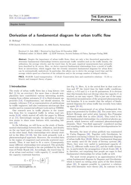
function (1) ismade.
The formulas for the non-congested regime can be either
expressed as non-trivial functions of the utilization
u i or the average queue length ΔNi
av (or the average density
ρ max
i ). They contain a fit parameter ɛ i , which reflects
effects of variations in the arrival flow and relates to the
efficiency of traffic signal operation in terms of synchronizing
with vehicle platoons. In the best case, delay times
are zero, which shows the great optimization potential for
traffic control in this regime.
In the congested regime, the number of delayed vehicles
grows in time, and the majority of vehicles is stopped several
times by the same traffic light. Therefore, the average
travel time does not only depend on the utilization u i , but
also on the average vehicle queue ΔNi
av (or the average
density ρ av
i ). Although the traffic light control can still improve
the average travel times by synchronizing with the
arrival of vehicles, the related efficiency effect is rather
limited.

10 The European Physical Journal B
Average Travel Time T i [T i
0 ]
10
8
6
4
2
0
0 0.2 0.4 0.6 0.8 1
Utilization u i
Fig. 5. (Color Online) Schematic illustration of the capacity
restraint function (1) that the Bureau of Public Roads recommends
to use [16] (solid line), together with analytical results
of this paper (dashed lines). Travel time T i is measured in units
of Ti 0 . The green long-dashed line shows that the travel time
diverges at u i ≈ 0.45, if two green phases during one cycle
and identical utilizations u 1 = u 2 of both associated road sections
are assumed, furthermore, if the parameters are set to
T los =0.1Ti
0 and δ =0.1. (A generalization to traffic operation
with more than two green phases is easily possible.) When
the cycle time is limited to a finite value Tcyc
max to avoid infinite
delay times in one of the vehicle queues, one will have growing
vehicle queues and increasing travel times in both road sections.
Therefore, the travel time can assume any value above
the lower dashed horizontal line. The link travel time is only
limited by the above dashed horizontal line, which corresponds
to the situation where the vehicle queue fills the road section
completely. Note that the capacity restraint function (solid
line) averages over all travel time measurements for a given
utilization u i. In the right part of the diagram this concerns
measurements that depend on the duration of congestion and
scatter between both horizontal dashed lines. Here, the curve
is shown for α i =0.5, β i =4,andA i/C i = u i/0.45.
In the oversaturated regime, the storage capacity of the
road section is fully occupied by delayed vehicles, which
obstructs the arrival flow. Therefore, the average travel
time of a road section reaches a constant maximum value.
Nevertheless, the travel time of vehicles increases further
in time due to spillover effects, which trigger the spreading
of congestion to upstream road sections. The actually
usable fraction of the green time period is described by
a parameter σ i . Synchronization can still reach some improvements.
The most favorable control is oriented at a
fluent upstream propagation of the little remaining free
space (the difference between ΔNi
max and ΔNi
min ). That
is, rather than minimizing the delay of downstream moving
vehicle platoons, one should now minimize the delay
in filling upstream moving gaps [42]. Furthermore, note
that the free travel time Ti 0 = L i /Vi
0 and the delay time
in the oversaturated regime are proportional to the length
L i of the road section, while the delay times in the undersaturated
and congested regimes are independent of L i .
Based on the above results, it is obvious that it cannot
be very successful to describe the travel time of a link by
a capacity restraint function which depends on A i /C i =
u i /u 0 i only. This basically means an averaging over data
that, in principle, are also dependent on the average queue
length ΔNi
av (or on the time passed since the onset of
congestion). It is, therefore, no wonder that empirical data
of travel times as a function of the utilization scatter so
enormously in the congested and oversaturated regimes
(see e.g. Ref. [27]), that a fitting of the data to functional
dependencies of any kind does not make much sense.
This has serious implications for transport modeling,
as capacity restraint functions such as formula (1)areused
for modeling route choice and, hence, for traffic assignment.
Based on the necessary revision of this formula and
comparable ones, all traffic scenarios based on these formulas
should be critically questioned. Given the computer
power of today, it would not constitute a problem to perform
a dynamic traffic assignment and routing based on
the more differentiated formulas presented in this paper.
6.1 Transferring the link-based urban fundamental
diagrams to an area-based one
We may finally ask ourselves, whether the above formulas
would also allow one to make predictions about the
average travel times and speeds for a whole area of an urban
traffic network, rather than for single road sections
(“links”) only. This would correspond to averaging over
the link-based fundamental diagrams of that area. For
the sake of simplicity, let us assume for a moment that
the parameters of all links would be the same, and derive
a velocity-density diagram from the relationship (A.9) between
average vehicle speed Vi
av and the capacity utilization
u i . Taking into account Vi 0 = L i /Ti
0 and dropping
the index i, wecanwrite
V av (u) = V 0 ln { 1+[1− f(u)]T cyc /T 0}
(1 − u)T cyc /T 0 + V 0 f(u) − u
1 − u ,
(74)
with f(u) =(1+δ)u. The cycle time
T cyc =
T los
1 − sf(u)
(75)
follows from equation (5), assuming s signal phases with
f i = f for simplicity. Note that the previous formulas for
ρ av
i denote the average density of delayed vehicles, while
the average density of all vehicles (i.e. delayed and freely
moving ones) is given by
ρ(u) = N(u)
L
N(u)/T (u)
= = A(u)
L/T (u) V av (u) =
u ̂Q
V av (u) , (76)
where N = AT = u ̂QT denotes the average number of
vehicles on a road section of length L. Plotting V av (u)
over ρ(u) finally gives a speed-density relationship V av (ρ).
We have now to address the question of what happens,
if we average over the different road sections of an urban

D. Helbing: Derivation of a fundamental diagram for urban traffic flow 11
area. Considering the heterogeneity of the link lengths L i ,
efficiencies ɛ i , utilizations u i , and densities ρ av
i , one could
think that the spread in the data would be enormous.
However, a considerable amount of smoothing results from
the fact that in- and outflows of links within the studied
urban area cancel out each other, and it does not matter
whether a vehicle is delayed in a particular link, or
in the previous or subsequent one. Therefore, the resulting
fundamental diagrams for urban areas are surprisingly
smooth [29,30]. The details of the curves, however, are expected
to depend not only on the average density, but also
on the density distribution, the signal operation schemes,
and potentially other factors as well.
When averaging over different links, we have to study
the effects of the averaging procedure on the density and
the speed. The density just averages linearly: thanks to
Little’s law [39], the formula (76) can also be applied to
an urban area, as long as the average number of vehicles
in it is stationary. However, as the link-based fundamental
diagram between the flow Q(ρ) =ρV av (ρ) andthedensity
ρ is convex, evaluating the flow at some average density
overestimates the average flow 2 . This also implies that,
when the relationship V av (ρ) is transferred from single
links to urban areas, the average speed is overestimated
for a given density, as reference [31] hasshown.
Despite this expected deviation in heterogeneous and
inhomogeneously used road networks, and despite the
many other simplifications, the curve V av (ρ) fitsempirical
data of the speed-density relation in an urban area
quite well. Figure 6 displays empirical data obtained for
the center of Yokohama [29] together with a fit of the theoretical
speed-density relationship V av (ρ), where only the
three parameters V 0 , δ, andV ∗ = L/T los were adjusted.
Surprisingly, the effects of network interactions could be
sufficiently well represented by a single parameter δ,which
relates to the efficiency ɛ of road sections according to
equation (32). This approximation seems to work in situations
close enough to a statistical equilibrium (when the
number of vehicles in the urban area does not change too
quickly).
In contrast, for an understanding of the spreading dynamics
of congestion patterns, we expect that one must
study the interaction between the flow dynamics and the
network structure. This difficult subject goes beyond the
scope of this paper and beyond what is doable at the moment,
but it will be interesting to address it in the future.
2 When averaging over speed values, they have to be
weighted by the number of vehicles concerned, i.e. by the density.
This comes down to determining an arithmetic average
of the flow values and dividing the result by the arithmetic
average of the related densities. Hence, an overestimation of
the average flow also implies an overestimation of the average
velocity. However, considering the curvature of Q(ρ) and
knowing the variability of the density ρ allows one to estimate
correction terms.
3 This corresponds to 10% extra green time, an average distance
between successive traffic lights of roughly 100 m (depending
on T los ), and an average of 3 traffic phases (which appears
plausible, considering that there are many one-way roads,
Speed (km/h)
35
30
25
20
15
10
5
0
0 0.02 0.04 0.06 0.08 0.1
Density (1/m)
Fig. 6. (Color online) Fundamental velocity-density relationship
for a central area of Yokohama. Small circles correspond
to empirical data by Kuwahara as evaluated by Daganzo
and Geroliminis [31]. The fit curve corresponds to the theoretically
derived equations (74) to(76), where the outflow
(discharge flow) ̂Q = 1800 veh./h/lane and the free speed
V 0 = 50 km/h have been fixed. The only fit parameters were
δ =0.1, T los /T 0 =1.4, and s =3 3 .
The author thanks for an inspiring presentation by Carlos
Daganzo, for useful comments by Stefan Lämmer, and intresting
discussions with Nikolas Geroliminis, who was also kind
enough to provide the empirical data from the center of Yokohama
displayed in Figure 6, see Figure 7 in reference [29].
He extracted these from original data of GPS-equipped taxis
by Prof. Masao Kuwahara from the University of Tokyo. The
fit of the theoretically predicted relationship to the empirical
data was carried out by Anders Johansson. Furthermore,
the author is grateful for partial support by the Daimler-
Benz Foundation Project 25-01.1/07 on BioLogistics, the VW
Foundation Project I/82 697, the NAP project KCKHA005
“Complex Self-Organizing Networks of Interacting Machines:
Principles of Design, Control, and Functional Optimization”,
and the ETH Competence Center ‘Coping with Crises in Complex
Socio-Economic Systems’ (CCSS) through ETH Research
Grant CH1-01-08-2.
Appendix A: Determination of average travel
times and velocities
Let f(x) be a function and w(x) a weight function. Then,
the average of the function between x = x 0 and x = x 1 is
which need less than 4 phases in one cycle time). Consequently,
all parameters are quite reasonable (see also Ref. [31]). Note
that effects of oversaturation did not have to be considered in
Figure 6. This is, in fact, consistent with pictures from Google
Earth.

12 The European Physical Journal B
defined as
∫x 1
dx ′ w(x ′ )f(x ′ )
x 0
∫x 1
. (A.1)
dx ′ w(x ′ )
x 0
In case of uniform arrivals of vehicles, we have a functional
relationship of the form f(x) =a + bx for the travel time,
and the weigth function is constant, i.e. w(x) =w. Here,
a = Ti 0,
x = ΔN i,andb =1/A i =1/(u i ̂Q i ). With x 0 =0
and x 1 = ΔNi
max , the formula for the average travel time
becomes
w[(ax 1 + bx 2 1 /2) − (ax 0 + bx 2 0 /2)]
= a + b x 1 + x 0
,
w(x 1 − x 0 )
2
(A.2)
wherewehaveused(x 2 1 − x 2 0 )=(x 1 − x 0 )(x 1 + x 0 ).
Inserting the above parameters, we obtain the previously
derived result
T i = T 0
i
+
ΔN
max
i
2u i ̂Qi
. (A.3)
When determining the average velocity Vi
av , the function
to average over is of the form f(x) =c/(a + bx), where
c = L i and the other parameters are as defined before. We
use the relationship
∫ x 1
dx ′ wc
a + bx ′ = wc (
)
ln |a + bx 1 |−ln |a + bx 0 |
b
x 0
= wc ∣ ∣ ∣∣∣
b ln a + bx 1 ∣∣∣
.
(A.4)
a + bx 0
Dividing this again by the normalization factor w(x 1 −x 0 )
and inserting the above parameters finally gives
V av
i
= L iu i ̂Qi
ΔN max
i
(
max
i
ln
1+ΔN ∣ u i ̂Qi Ti
0 ∣ ≈ L i
Ti
0 1 −
ΔN
max
i
2u i ̂Qi T 0
i
)
,
(A.5)
wherewehaveusedln(1+x) ≤ x − x 2 /2. This formula
corrects the naive formula
V av
i
≈ L i
T i
=
T 0
i
+
L i
ΔN max
1
2u i ̂Qi
≈ L i
T 0
i
(
1 −
)
max
ΔN1
, (A.6)
2u i ̂Qi Ti
0
wherewehaveused1/(1 + x) ≈ 1 − x. Therefore, the
above Taylor approximations of both formulas agree, but
higher-order approximations would differ. The formulas
in the main part of the paper result for Ni
av = Ni max /2,
which corresponds to the case δ i = 0 (i.e. f i − u i ).
Generalizing the above approach to the case δ i > 0,
we must split up the integrals into one over wc/(a + bx ′ )
extending from x 0 =0tox 1 = ΔNi
max and another one
over wc/a from x 1 = ΔNi max to x 2 =(1− u i )A i T cyc =
(1−u i )u i ̂Qi T cyc , where the specifications of a, b, andc are
unchanged. Taking into account Vi 0 = L i /Ti 0,thisgives
V av
i
= wL iu i ̂Qi ln |1+ΔN max
i /(u i ̂Qi T 0
i )| + Z
w(1 − u i )u i ̂Qi T cyc , (A.7)
where
Z = wV 0
i [(1 − u i )u i ̂Qi T cyc − ΔN max
i ]. (A.8)
Considering equation (15), we get
V av
i =
L i
(1 − u i )T cyc
ln
(
1+(1− f i ) T cyc
T 0
i
)
+ Vi
0 f i − u i
.
1 − u i
(A.9)
In second-order Taylor approximation, this results in
[ ( 1 −
Vi av ≈ Vi
0 fi
1 − (1 − f )
i)T cyc
1 − u i 2Ti
0 + f ]
i − u i
,
1 − u i
(A.10)
which can also be derived from equation (A.6), considering
equation (15) and the percentage of delayed vehicles,
which is given by equation (19).Thesameresultfollows
from
V av
i =
T 0
i
L i
+ T av
i
≈ V 0
i
together with equation (21).
References
(1 − T i
av )
Ti
0
(A.11)
1. D.C. Gazis, Traffic Theory (Kluwer Academic, Boston,
2002)
2. J. Esser, M. Schreckenberg, Int. J. Mod. Phys. B 8, 1025
(1997)
3. P.M. Simon, K. Nagel, Phys. Rev. E 58, 1286 (1998)
4. K. Nagel, Multi-Agent Transportation Simulations, see
http://www2.tu-berlin.de/fb10/ISS/FG4/archive/
sim-archive/publications/book/
5. M. Hilliges, W. Weidlich, Transpn. Res. B 29, 407 (1995)
6. D. Helbing, J. Siegmeier, S. Lämmer, Networks and
Heterogeneous Media 2, (2007)
7. M. Cremer, J. Ludwig, Math. Comput. Simul. 28, 297ff
(1986)
8. C.F. Daganzo, Transpn. Res. B 29, 79 (1995)
9. T. Nagatani, Phys. Rev. E 48, 3290 (1993)
10. D. Chowdhury, A. Schadschneider, Phys. Rev. E 59,
R1311 (1999)
11. O. Biham, A.A. Middleton, D. Levine, Phys. Rev. A 46,
R6124 (1992)
12. J.-F. Zheng, Z.-Y. Gao, X.-M. Zhao, Phys. Stat. Mech.
Appl. 385, 700 (2007)
13. N.A. Irwin, M. Dodd, H.G. Von Cube, Highway Research
Board Bulletin 347, 258 (1961)
14. R.J. Smock, Highway Research Board Bulletin 347, 60
(1962)
15. W.W. Mosher, Highway Research Record 6, 41 (1963)
16. Bureau of Public Roads, Traffic Assignment Manual
(US Dept. of Commerce, Urban Planning Division,
Washington, D.C., 1964)
17. T.J. Soltmann, Highway Research Record 114, 122 (1965)
18. K.B. Davidson, in Proceedings of the 3rd ARRB
Conference, Part 1 (Australian Road Research Board,
Melbourne, 1966), pp. 183–194

D. Helbing: Derivation of a fundamental diagram for urban traffic flow 13
19. R.J. Smeed, Traffic Engineering and Control 8, 455 (1966)
20. K.R. Overgaard, Traffic Quarterly, 197 (1967)
21. J.M. Thomson, Traffic Engineering and Control 8, 721
(1967)
22. J.G. Wardrop, Traffic Engineering and Control 9, 528
(1968)
23. Y. Zahavi, Traffic Engineering and Control 14, (1972)
24. R. Akcelik, Australian Road Research 21, 49 (1991)
25. K.M. Lum, H.S.L. Fan, S.H. Lam, P. Olszewski,
J. Transpn. Eng. 124, 213 (1998)
26. H.M. Zhang, Transpn. Res. Rec. 1676, 109 (1999)
27. H. Tu, Monitoring Travel Time Reliability on Freeways,
Ph.D. thesis, Delft University of Technology, (2008)
28. C.F. Daganzo, Transport. Res. B 41, 49 (2007)
29. N. Geroliminis, C.F. Daganzo, Transpn. Res. B 42, 759
(2008)
30. N. Geroliminis, C.F. Daganzo, Macroscopic modeling of
traffic in cities, TRB 86th Annual Meeting, Paper
#07-0413, Washington D.C. (2007)
31. C.F. Daganzo, N. Geroliminis, An analytical approximation
for the macroscopic fundamental diagram of urban
traffic, accepted for publication (2008)
32. J.W. Godfrey, Traffic Engineering and Control 11, 323
(1969)
33. R. Herman, I. Prigogine, Science 204, 148 (1979)
34. R. Herman, S. Ardekani, Transportation Science 18, 101
(1984)
35. M. Eichler, C.F. Daganzo, Transportation Research B 40,
731 (2006)
36. D. Helbing, Rev. Mod. Phys. 73, 1067 (2001)
37. D. Helbing, M. Treiber, A. Kesting, M. Schönhof,
Theoretical vs. empirical classification and prediction of
congested traffic states, Eur. Phys. J. B, accepted for publication
(2009), see e-print
http://arxiv.org/abs/0903.0929
38. G.B. Whitham, Linear and Nonlinear Waves (Wiley, New
York, 1974)
39. R. Hall, Queueing Methods for Service and Manufacturing
(Prentice Hall, Upper Saddle River, NJ, 1991)
40. D. Helbing, J. Phys. A: Math. Gen 36, L593 (2003)
41. D. Helbing, A. Mazloumian, Operation regimes and sloweris-faster
effect in the control of traffic intersections, submitted
(2008), see e-print
http://arxiv.org/abs/0903.0926
42. D. Helbing, T. Seidel, S. Lämmer, K. Peters, in
Econophysics and Sociophysics, edited by B.K.
Chakrabarti, A. Chakraborti, A. Chatterjee (Wiley,
Weinheim, 2006), p. 552