2012-03-27_CRAM Field Book Riverine

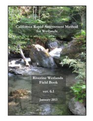
California Rapid Assessment Method 

for Wetlands 

Riverine Wetlands 

Field Book 

ver. 6.0 

March 2012

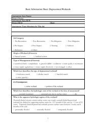
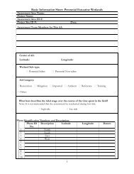
Basic Information Sheet: Riverine Wetlands 

CRAM Site ID: 

Project Site ID: 

Assessment Area Name: 

Project Name: 

Date (m/d/y) 

Assessment Team Members for This AA: 

Average Bankfull Width: 

Approximate Length of AA (10 times bankfull width, min 100 m, max 200 m): 

Upstream Point Latitude: 

Downstream Point Latitude: 

Longitude: 

Longitude: 

Wetland Sub-type: 

Confined 

Non-confined 

AA Category: 

Restoration Mitigation Impacted Ambient Reference Training 

Other: 

Did the river/stream have flowing water at the time of the assessment yes no 

What is the apparent hydrologic flow regime of the reach you are assessing 

The hydrologic flow regime of a stream describes the frequency with which the channel conducts 

water. Perennial streams conduct water all year long, whereas ephemeral streams conduct water only 

during and immediately following precipitation events. Intermittent streams are dry for part of the year, 

but conduct water for periods longer than ephemeral streams, as a function of watershed size and water 

source. 

perennial intermittent ephemeral 

2

Photo Identification Numbers and Description: 

Photo ID Description Latitude Longitude Datum 

No. 

1 Upstream 

2 Middle Left 

3 Middle Right 

4 Downstream 

5 

6 

7 

8 

9 

10 

Site Location Description: 

Comments: 

3

Scoring Sheet: Riverine Wetlands 

AA Name: 

(m/d/y) 

Attribute 1: Buffer and Landscape Context 

Aquatic Area Abundance Score (D) 

Alpha. Numeric 

Comments 

Buffer: 

Buffer submetric A: 

Percent of AA with Buffer 

Alpha. 

Numeric 

Buffer submetric B: 

Average Buffer Width 

Buffer submetric C: 

Buffer Condition 

Raw Attribute Score = D+[ C x (A x B) ½ ] ½ 

(use numerical value to nearest whole integer) 

Attribute 2: Hydrology 

Water Source 

Channel Stability 

Hydrologic Connectivity 

Alpha. 

Raw Attribute Score = sum of numeric scores 

Attribute 3: Physical Structure 

Structural Patch Richness 

Topographic Complexity 

Alpha. 


Attribute 4: Biotic Structure 

Plant Community Composition (based on sub-metrics A-C) 

Plant Community submetric A: 

Number of plant layers 

Plant Community submetric B: 

Number of Co-dominant species 

Plant Community submetric C: 

Percent Invasion 

Plant Community Composition 

(average of submetrics A-C rounded to nearest whole integer) 

Horizontal Interspersion 

Vertical Biotic Structure 

Alpha. 

Numeric 


4 

Numeric 

Numeric 

Overall AA Score (average of four final Attribute Scores) 

Final Attribute Score = 

(Raw Score/24) x 100 






(Raw Score/36) x 100

Identify Wetland Type 

Figure 1: Flowchart to determine wetland type and sub-type. 

5

Riverine Wetlands (Including Closely Associated Riparian Areas) 

A riverine wetland consists of the riverine channel and its active floodplain, plus any portions of the 

adjacent riparian areas that are likely to be strongly linked to the channel and immediate floodplain 

through bank stabilization and allochthonous organic material (productivity) inputs. An active floodplain is 

defined as the relatively level area that is periodically flooded, as evidenced by deposits of fine sediment, 

wrack lines, vertical zonation of plant communities, etc. The water level that corresponds to incipient 

flooding can vary depending on flow regulation and whether the channel is in equilibrium with water and 

sediment supplies. Under equilibrium conditions, the usual high water contour that marks the inboard 

margin of the floodplain (i.e., the margin nearest the thalweg of the channel) corresponds to the height of 

bankfull flow, which typically has a recurrence interval of about 1.5 to 2.0 years under mesic climate 

conditions. The active floodplain can include broad areas of vegetated and non-vegetated bars and low 

benches among the distributaries of deltas and braided channel systems. The active floodplain does not 

include terraces that are geomorphologically disconnected from channel-forming processes, although 

riparian areas along terrace margins may be included as part of the floodplain. Vegetated wetlands can 

develop along the channel bottoms of intermittent and ephemeral streams during the dry season. Dry 

season assessment in these systems therefore includes the channel beds. However, the channel bed is 

excluded from the assessment when it contains non-wadeable flow. To help standardize the assessment of 

riverine wetlands, the assessments should be restricted to the dry season. 

There may be a limit to the applicability of this module in low order (i.e., headwater) streams, in very arid 

environments, and in desert streams that tend not to support species-rich plant communities with complex 

horizontal and vertical structure. CRAM may be systematically biased against such naturally simple riverine 

systems. In addition, this module is has limited application in river reaches with extremely broad 

floodplains, such as those which occur where large rivers occupy valleys with very low channel slopes, or 

near coastal embayments or the ocean, unless the extent of the floodplain included in the Assessment Area 

is limited to an area less than about two times bankfull width on each side of the channel (see below). 

Riverine wetlands are further classified as confined or non-confined, based on the ratio of valley width to 

channel bankfull width (see Figure 2 below). Channels can also be entrenched, based on the ratio of flood 

prone width to bankfull width (Figure 2 below). Entrenchment affects hydrologic connectivity. A channel 

can also be considered confined by artificial levees and urban development if the average distance across 

the channel at bankfull is more than half the distance between the levees or more than half the width of 

the non-urbanized lands that border the stream course. This assumes that the channel would not be 

allowed to migrate past the levees or into the urban development, or that levee breaches will be repaired. 

6

Valley Width 

A 

B 

Bankfull Width 

C 

D 

Figure 2: Illustrations of alternative conditions of riverine confinement and entrenchment. (A) nonconfined, 

entrenched, (B) non-confined, not entrenched, (C) confined, not entrenched, and 

(D) confined, entrenched riverine. 

Non-confined Riverine Sub-type: 

In non-confined riverine systems, the width of the valley across which the system can migrate without 

encountering a hillside, terrace, or other feature that is likely to prevent further migration is at least twice 

the average bankfull width of the channel. Non-confined riverine systems typically occur on alluvial fans 

and plains, deltas in lakes, and along broad valleys. 

Confined Riverine Sub-type: 

In confined riverine systems, the width of the valley across which the system can migrate without 

encountering a hillside, terrace, man-made levee, or urban development is less than twice the average 

bankfull width of the channel. 

Special Note: 

*Entrenchment varies naturally with channel confinement. Channels in steep canyons naturally tend to be confined, and tend 

to have small entrenchment ratios indicating less hydrologic connectivity. Assessments of hydrologic connectivity based on 

entrenchment must therefore be adjusted for channel confinement. It is essential that the riverine AA be further classified as 

confined or unconfined, based on the definitions provided 

7

Establish the Assessment Area (AA) 

For a riverine wetland, the AA should begin at a hydrological or geomorphic break in form or structure of 

the channel that corresponds to a significant change in flow regime or sediment regime, as guided by 

Tables 1 and 2. If no such break exists, then the AA can begin at any point near the middle of the wetland. 

For ambient surveys, the AA should begin at the point drawn at random from the sample frame. From 

this beginning, the AA should extend upstream or downstream for a distance ten times (10x) the average 

bankfull width of the channel, but at least 100 m, and for a distance no longer than 200 m. In any case, the 

AA should not extend upstream of any confluence that obviously increases the downstream sediment 

supply or flow, or if the channel in the AA is obviously larger below the confluence than above it. The 

AAs should include both sides of wadeable channels, but only one side of channels that cannot be safely 

crossed by wading. 

All types of wetlands can have adjacent riparian areas that benefit the wetlands. Riparian areas play a 

particularly important role in the overall form and function of riverine wetlands. Riverine wetlands are 

generally highly influenced by the allochthonous organic material input from riparian areas that support 

aquatic food webs. Also, the large woody debris provided by riparian areas can be essential to maintaining 

riverine geomorphology, such as pools and riffles, as well as the associated ecological services, such as the 

support of anadromous fishes. Conservation policies and practices commonly associate riparian functions 

with riverine wetlands more than other wetland types. 

Therefore, the riverine AA should extend landward from the foreshore of the floodplain (located at the 

bankfull width) to include the adjacent riparian area that probably accounts for bank stabilization and most 

of the direct allochthonous inputs of leaves, limbs, insects, etc., into the channel, and its immediate 

floodplain. Any trees or shrubs that directly contribute allochthonous material to the channel and its 

immediate floodplain should be included in the AA in their entirety (Figure 3). The AA can include 

topographic floodplain benches, interfluves, paleo-channels, meander cutoffs, and other features that are 

at least semi-regularly influenced by fluvial processes associated with the main channel of the AA. It can 

also include adjacent areas such as terrace margins that support vegetation that is likely to directly provide 

allochthonous inputs. 

Special Note: 

*The opposing sides (different banks) of a riverine AA can have different riparian widths, based on differences in plant 

architecture and topography. 

*The minimum width of the AA should extend no less than two meters (2 m) from the bankfull channel margin. 

*Where the module is applied to riverine wetlands that occupy very broad floodplains (for example, where floodplains are > 

10X or 20X the average channel width), CRAM does not adequately address the multiple dynamic processes that occur on 

the extensive floodplains, and the riverine AA must be limited to the area that directly influences the channel. While it is 

clear that during floods the entire floodplain may contribute allochthonous material to the wetland ecosystem, and while it is 

also clear that very broad floodplains may significantly influence the hydrological dynamics of large rivers in flood, these factors 

were not incorporated into the development of the Riverine module. In order to allow the module to be applied to these 

wetlands, the AA should be limited to the floodplain area that immediately affects the channel, which is defined for the 

purposes of CRAM as the area no more than two times the bankfull width on each side of the channel. However, within that 

distance, if a topographic feature is encountered, use this feature along with standard CRAM guidance to define the edge of the 

AA. 

*In systems located in a steep valley which lack an obvious active floodplain, set the lateral extent of the AA a distance of no 

more than two times the bankfull width on each side of the channel to include the adjacent riparian area that probably 

accounts for bank stabilization and most of the direct allochthonous inputs of leaves, limbs, insects, etc., into the channel. 

8

Figure 3: Diagram of the lateral extent of a riverine AA that includes the portion of the 

riparian area that can help stabilize the channel banks and that can readily provide 

allochthonous inputs of plant matter, insects, etc. to the channel and its immediate 

floodplain. 

9

Table 1: Examples of features that should be used to delineate AA boundaries for 

Riverine wetlands. 

• major changes in riverine entrenchment, confinement, degradation, aggradation, 

slope, or bed form 

• major channel confluences 

• diversion ditches 

• end-of-pipe large discharges 

• water falls 

• open water areas more than 30 m wide on average or broader than the wetland 

• transitions between wetland types 

• weirs, culverts, dams, drop- structures, levees, and other flow control, grade 

control, or water height control structures 

Table 2: Examples of features that should not be used to delineate AAs. 

• at-grade, unpaved, single-lane, infrequently used roadways or crossings 

• bike paths and jogging trails at grade 

• bare ground within what would otherwise be the AA boundary 

• equestrian trails 

• fences (unless designed to obstruct the movement of wildlife) 

• property boundaries, unless access is not allowed 

• riffle (or rapid) – glide – pool transitions in a riverine wetland 

• spatial changes in land cover or land use along the wetland border 

• state and federal jurisdictional boundaries 

Table 3: Recommended maximum and minimum AA sizes for the Riverine wetland type. 

Note: Wetlands smaller than the recommended AA sizes can be assessed in their entirety. 

Wetland Type 

Recommended AA Size 

Confined and Nonconfined 

Riverine 

Recommended length is 10x average bankfull channel width; 

maximum length is 200 m; minimum length is 100 m. 

10

Attribute 1: Buffer and Landscape Context 

Metric 1: Riparian Continuity (Aquatic Area Abundance) 

Definition: The Riparian Continuity metric for a riverine Assessment Area is assessed in terms 

of its spatial association with other areas of aquatic resources. Wetlands close to each other have 

a greater potential to interact ecologically and hydrologically, and such interactions are generally 

beneficial. 

For riverine wetlands, aquatic area abundance is assessed as the continuity of the riparian 

corridor over a distance of 500 m upstream and 500 m downstream of the AA. While riparian 

areas upstream and downstream generally reflect the overall health of the riverine system, of 

special concern for this metric is the ability of wildlife to enter the riparian area from outside of it 

at any place within 500 m of the AA, and to move easily through adequate cover along the 

riparian corridor through the AA from upstream and downstream. This metric is assessed as the 

total length of unfavorable habitat (defined by the “non-buffer land covers” in Table 6) that 

interrupts the riparian corridor within 500 m upstream or downstream of the AA. “Non-buffer 

land covers” occupying less than 10 m of stream length are disregarded in this metric. 

It should be noted that this metric adopts the “non-buffer land cover” types in Table 6 as 

indications of habitat conditions that break or disrupt ecological and hydrological continuity. 

This metric explicitly addresses the connectivity of the AA with the riparian areas upstream and 

downstream, and the “non-buffer land covers” are considered as indicators of conditions that 

break this continuity. This metric does not address the AA buffer condition, which is addressed in 

the following metric. 

Special Note: 

*Assume the riparian width is the same upstream and downstream as it is for the AA, unless a substantial 

change in width is obvious for a distance of at least 100 m. 

*To be a concern, a “non-buffer land cover” segment must break or sever the continuity of the riparian area for a 

length of at least 10 meters on at least one side of the channel upstream or downstream from the AA. 

*For the purpose of assessing aquatic area abundance for riverine wetlands, open water is considered part of the 

riparian corridor. This acknowledges the role the riparian corridors have in linking together aquatic habitats and 

in providing habitat for anadromous fish and other wildlife. 

*A bridge crossing the stream that is at least 10 m wide will typically interrupt the riparian corridor on both sides 

of the stream, thus the crossing width is counted twice, once for the right bank and once for the left bank. 

*For wadeable systems, assess both sides of the channel upstream and downstream from the AA. 

*For systems that cannot be waded, only assess the side of the channel that has the AA, upstream and 

downstream from the AA. 

11

Step 1 

Step 2 

Step 3 

Table 4: Steps to assess Riparian Continuity for riverine wetlands. 

Extend the average width of the AA 500 m upstream and downstream, regardless 

of the land cover types that are encountered (see Figure 4). 

Using the site imagery, identify all the places where “non-buffer land covers” (see 

Table 6) at least 10 m wide interrupt the riparian area within the average width of 

your AA on either side of the channel in the extended AA. Disregard 

interruptions of the riparian corridor that are less than 10 m wide (measured 

parallel to the stream). Do not consider open water as an interruption. For onesided 

riverine AAs, assess only one side of the system 

Estimate the length of each “non-buffer” segment identified in Step 2, and enter 

the estimates in the worksheet for this metric. 

Assessment Area (AA) 

Extended AA 

Non-buffer Land Cover Segments 

AA 

500 m 

Figure 4: Diagram of method to assess Riparian Continuity of riverine wetlands. This example shows that 

about 400 m of “non-buffer land cover” crosses about half of the riparian corridor within 500 m 

downstream of the AA. This is due to the large parking lot on the south side of the stream in addition to 

two bridge crossings. There is a 20 m break in the riparian corridor upstream of the AA due to a bridge 

crossing (10 m for each side of the stream). 

Worksheet for Riparian Continuity Metric for Riverine Wetlands 

Lengths of Non-buffer Segments For 

Distance of 500 m Upstream of AA 

Lengths of Non-buffer Segments For 

Distance of 500 m Downstream of AA 

Segment No. Length (m) Segment No. Length (m) 

1 1 

2 2 

3 3 

4 4 

5 5 

Upstream Total Length 

Downstream Total Length 

12

Table 5: Rating for Riparian Continuity for Riverine wetlands. 

Rating 

A 

B 

C 

D 

For Distance of 500 m Upstream of 

AA: 

The combined total length of all nonbuffer 

segments is less than 100 m for 

wadeable systems (“2-sided” AAs); 50 m 

for non-wadeable systems (“1-sided” 

AAs). 


segments is less than 100 m for “2- 

sided” AAs; 50 m for “1-sided” AAs. 


segments is between 100 m and 200 

m for “2-sided” AAs; 50 m and 100 m for 

“1-sided” AAs. 


segments is between 100 m and 200 

m for “2-sided” AAs; 50 m and 100 m for 

“1-sided” AAs. 

The combined total length of non-buffer 

segments is greater than 200 m for “2- 

sided” AAs; greater than 100 m for “1- 

sided” AAs. 

any condition 

OR 

OR 

For Distance of 500 m Downstream of AA: 

The combined total length of all non-buffer 

segments is less than 100 m for wadeable systems 

(“2-sided” AAs); 50 m for non-wadeable systems 

(“1-sided” AAs). 


segments is between 100 m and 200 m for “2- 

sided” AAs; 50 m and 100 m for “1-sided” AAs. 


segments is less than 100 m for “2-sided” AAs; is 

less than 50 m for “1-sided” AAs. 


segments is between 100 m and 200 m for “2- 

sided” AAs; 50 m and 100 m for “1-sided” AAs. 

any condition 

The combined total length of non-buffer 

segments is greater than 200 m for “2-sided” 

AAs; greater than 100 m for “1-sided” AAs. 

13

Metric 2: Buffer 

Definition: The buffer is the area adjoining the AA that is in a natural or semi-natural state and currently 

not dedicated to anthropogenic uses that would severely detract from its ability to entrap contaminants, 

discourage forays into the AA by people and non-native predators, or otherwise protect the AA from 

stress and disturbance. 

To be considered as buffer, a suitable land cover type must be at least 5 m wide starting at the edge of the 

AA extending perpendicular to the channel and extend along the perimeter of the AA (measured parallel 

to the channel) for at least 5 m. The maximum width of the buffer is 250 m. At distances beyond 250 m 

from the AA, the buffer becomes part of the landscape context of the AA. 

Special Note: 

*Any area of open water at least 30 m wide that is adjoining the AA, such as a lake, large river, or large slough, is not 

considered in the assessment of the buffer. Such open water is considered to be neutral, and is neither part of the wetland nor 

part of the buffer. There are three reasons for excluding large areas of open water (i.e., more than 30 m wide) from 

Assessment Areas and their buffers. 

1) Assessments of buffer extent and buffer width are inflated by including open water as a part of the buffer. 

2) While there may be positive correlations between wetland stressors and the quality of open water, quantifying 

water quality generally requires laboratory analyses beyond the scope of rapid assessment. 

3) Open water can be a direct source of stress (i.e., water pollution, waves, boat wakes) or an indirect source of stress 

(i.e., promotes human visitation, encourages intensive use by livestock looking for water, provides dispersal 

for non-native plant species), or it can be a source of benefits to a wetland (e.g., nutrients, propagules of 

native plant species, water that is essential to maintain wetland hydroperiod, etc.). 

*However, any area of open water that is within 250 m of the AA but is not directly adjoining the AA is considered part of 

the buffer. 

Submetric A: Percent of AA with Buffer 

Definition: This submetric is based on the relationship between the extent of buffer and the functions 

provided by aquatic areas. Areas with more buffer typically provide more habitat values, better water 

quality and other valuable functions. This submetric is scored by visually estimating from aerial imagery 

(with field verification) the percent of the AA that is surrounded by at least 5 meters of buffer land cover 

(Figure 5). The upstream and downstream edges of the AA are not included in this metric, only the edges 

parallel to the stream. 

14

Figure 5: Diagram of approach to 

estimate Percent of AA with Buffer for 

Riverine AAs. The white line is the edge 

of the AA, the red line indicates where 

there is less than 5 meters of buffer land 

cover adjacent to the AA, while the green 

line indicates where buffer is present. In 

this example 55% of the AA has buffer. 

Table 6: Guidelines for identifying wetland buffers and breaks in buffers. 

Examples of Land Covers 

Included in Buffers 

• at-grade bike and foot 

trails, or trails (with light 

traffic) 

• horse trails 

• natural upland habitats 

• nature or wildland parks 

• range land and pastures 

• railroads (with 

infrequent use: 2 trains 

per day or less) 

• roads not hazardous to 

wildlife, such as seldom 

used rural roads, forestry 

roads or private roads 

• swales and ditches 

• vegetated levees 

Examples of Land Covers Excluded from Buffers 

Notes: buffers do not cross these land covers; areas 

of open water adjacent to the AA are not included in 

the assessment of the AA or its buffer. 

• commercial developments 

• fences that interfere with the movements of wildlife 

(i.e. food safety fences that prevent the movement 

of deer, rabbits and frogs) 

• intensive agriculture (row crops, orchards and 

vineyards) 

• golf courses 

• paved roads (two lanes or larger) 

• active railroads (more than 2 trains per day) 

• lawns 

• parking lots 

• horse paddocks, feedlots, turkey ranches, etc. 

• residential areas 

• sound walls 

• sports fields 

• urbanized parks with active recreation 

• pedestrian/bike trails (with heavy traffic) 

15

Percent of AA with Buffer Worksheet. 

In the space provided below make a quick sketch of the AA, or perform the assessment directly on the 

aerial imagery; indicate where buffer is present, estimate the percentage of the AA perimeter providing 

buffer functions, and record the estimate amount in the space provided. 

Percent of AA with Buffer: % 

Table 7: Rating for Percent of AA with Buffer. 

Rating 

A 

B 

C 

D 

Alternative States 

(not including open-water areas) 

Buffer is 75 - 100% of AA perimeter. 

Buffer is 50 – 74% of AA perimeter. 



16

Submetric B: Average Buffer Width 

Definition: The average width of the buffer adjoining the AA is estimated by averaging the lengths of 

eight straight lines drawn at regular intervals around the AA from its perimeter outward to the nearest 

non-buffer land cover or 250 m, which ever is first encountered. It is assumed that the functions of the 

buffer do not increase significantly beyond an average width of about 250 m. The maximum buffer width 

is therefore 250 m. The minimum buffer width is 5 m, and the minimum length of buffer along the 

perimeter of the AA is also 5 m. Any area that is less than 5 m wide and 5 m long is too small to be a 

buffer. See Table 6 above for more guidance regarding the identification of AA buffers. 

Table 8: 

Steps to estimate Buffer Width for riverine wetlands 

Step 1 

Step 2 

Step 3 

Step 4 

Step 5 

Identify areas in which open water is directly adjacent to 

the AA, with

Figure 6: Diagram of approach to 

estimate Average Buffer Width for 

Riverine AAs. Continuing with the 

example from above, draw 8 lines evenly 

distributed within the buffer. The lines 

end in this example when they encounter 

active row crop agriculture, a lawn, and 

some fencing that restricts wildlife 

movement. 

Worksheet for calculating average buffer width of AA 

Line 

A 

B 

C 

D 

E 

F 

G 

H 

Average Buffer Width 

Buffer Width (m) 

Table 9: Rating for average buffer width. 

Rating 


A Average buffer width is 190 – 250 m. 

B Average buffer width 130 – 189 m. 

C Average buffer width is 65 – 129 m. 

D Average buffer width is 0 – 64 m. 

18

Submetric C: Buffer Condition 

Definition: The condition of a buffer is assessed according to the extent and quality of its vegetation 

cover, the overall condition of its substrate, and the amount of human visitation. Buffer conditions are 

assessed only for the portion of the wetland border that has already been identified as buffer (i.e., as in 

Figure 7). Thus, evidence of direct impacts (parking lots, buildings, etc.) by people are excluded from this 

metric, because these features are not included as buffer land covers; instead these impacts are included in 

the Stressor Checklist. If there is no buffer, assign a score of D. 

Figure 7: Diagram of method to assess 

Buffer Condition for Riverine AAs. 

Continuing with the example from above, 

this submetric assesses the condition of the 

buffer only where it was found to be 

present in the two previous steps (the 

shaded areas shown). 

Table 10: Rating for Buffer Condition. 

Rating 

A 

B 


Buffer for AA is dominated by native vegetation, has undisturbed soils, and is 

apparently subject to little or no human visitation. 

Buffer for AA is characterized by an intermediate mix of native and non-native 

vegetation (25% to 75% non-native), but mostly undisturbed soils and is apparently 

subject to little or low impact human visitation. 

OR 

Buffer for AA is dominated by native vegetation, but shows some soil disturbance and is 

apparently subject to little or low impact human visitation. 

C 

D 

Buffer for AA is characterized by substantial (>75%) amounts of non-native vegetation 

AND there is at least a moderate degree of soil disturbance/compaction, and/or there is 

evidence of at least moderate intensity of human visitation. 

Buffer for AA is characterized by barren ground and/or highly compacted or otherwise 

disturbed soils, and/or there is evidence of very intense human visitation. 

19

Metric 1: Water Source 

Attribute 2: Hydrology 

Definition: Water sources directly affect the extent, duration, and frequency of the hydrological dynamics 

within an Assessment Area. Water sources include direct inputs of water into the AA as well as any 

diversions of water from the AA. Diversions are considered a water source because they affect the ability 

of the AA to function as a source of water for other habitats while also directly affecting the hydrologic 

regime of the AA. 

A water source is direct if it supplies water mainly to the AA, rather than to areas through which the water 

must flow to reach the AA. Natural, direct sources include rainfall, ground water discharge, and flooding 

of the AA due to naturally high riverine flows. Examples of unnatural, direct sources include stormdrains 

that empty directly into the AA or into an immediately adjacent area. Indirect sources that should not be 

considered in this metric include large regional dams that have ubiquitous effects on broad geographic 

areas of which the AA is a small part. However, the effects of urbanization on hydrological dynamics in 

the immediate watershed containing the AA (“hydromodification”) are considered in this metric; because 

hydromodification both increases the volume and intensity of runoff during and immediately after rainy 

season storm events and reduces infiltration that supports base flow discharges during the drier seasons 

later in the year. 

Engineered hydrological controls such as weirs, flashboards, grade control structures, check dams, etc., can 

serve to demarcate the boundary of an AA but they are not considered water sources. 

Natural sources of water for riverine wetlands include precipitation, snow melt, groundwater, and riverine 

flows. Whether the wetlands are perennial or seasonal, alterations in the water sources result in changes in 

either the high water or low water levels. Such changes can be assessed based on the patterns of plant 

growth along the wetland margins or across the bottom of the wetlands. 

To score this metric use site aerial imagery and any other information collected about the region or 

watershed surrounding the AA to assess the water source in a 2 km area upstream of the AA (Table 11). 

2 km 

Figure 8: Diagram of approach to assess 

water sources affecting a CRAM AA 

showing an oblique view of the watershed. 

After identifying the portion of the aerial 

imagery that constitutes the contributing 

watershed region for the AA, assess the 

condition of the water source in a 2 km 

region (represented by yellow lines) 

upstream of the AA (represented with green 

box). 

20

Table 11: Rating for Water Source. 

Rating 

A 

B 

C 

D 


Freshwater sources that affect the dry season condition of the AA, such as 

its flow characteristics, hydroperiod, or salinity regime, are precipitation, 

snow melt, groundwater, and/or natural runoff, or natural flow from an 

adjacent freshwater body, or the AA naturally lacks water in the dry 

season. There is no indication that dry season conditions are 

substantially controlled by artificial water sources. 

Freshwater sources that affect the dry season condition of the AA are 

mostly natural, but also obviously include occasional or small effects of 

modified hydrology. Indications of such anthropogenic inputs include 

developed land or irrigated agricultural land that comprises less than 20% 

of the immediate drainage basin within about 2 km upstream of the AA, 

or that is characterized by the presence of a few small stormdrains or 

scattered homes with septic systems. No large point sources or dams 

control the overall hydrology of the AA. 

Freshwater sources that affect the dry season conditions of the AA are 

primarily urban runoff, direct irrigation, pumped water, artificially 

impounded water, water remaining after diversions, regulated releases of 

water through a dam, or other artificial hydrology. Indications of 

substantial artificial hydrology include developed or irrigated agricultural 

land that comprises more than 20% of the immediate drainage basin 

within about 2 km upstream of the AA, or the presence of major point 

source discharges that obviously control the hydrology of the AA. 

OR 

Freshwater sources that affect the dry season conditions of the AA are 

substantially controlled by known diversions of water or other 

withdrawals directly from the AA, its encompassing wetland, or from its 

drainage basin. 

Natural, freshwater sources that affect the dry season conditions of the 

AA have been eliminated based on the following indicators: 

impoundment of all possible wet season inflows, diversion of all dryseason 

inflow, predominance of xeric vegetation, etc. 

21

Metric 2: Channel Stability 

Definition: For riverine systems, the patterns of increasing and decreasing flows that are associated with 

storms, releases of water from dams, seasonal variations in rainfall, or longer term trends in peak flow, 

base flow, and average flow are very important. The patterns of flow, in conjunction with the kinds and 

amounts of sediment that the flow carries or deposits, largely determine the form of riverine systems, 

including their floodplains, and thus also control their ecological functions. Under natural conditions, the 

opposing tendencies for sediment to stop moving and for flow to move the sediment tend toward a 

dynamic equilibrium, such that the form of the channel in cross-section, plan view, and longitudinal profile 

remains relatively constant over time (Leopold 1994). Large and persistent changes in either the flow 

regime or the sediment regime tend to destabilize the channel and cause it to change form. Such regime 

changes can be associated with upstream land use changes, alterations of the drainage network of which 

the channel of interest is a part, and climatic changes. A riverine channel is an almost infinitely adjustable 

complex of interrelations among flow, width, depth, bed resistance, sediment transport, and riparian 

vegetation. Change in any of these factors will be countered by adjustments in the others. 

Channel stability is assessed as the degree of channel aggradation (i.e., net accumulation of sediment on the 

channel bed causing it to rise over time), or degradation (i.e., net loss of sediment from the bed causing it 

to be lower over time). The degree of channel stability can be assessed based on field indicators. There is 

much interest in channel entrenchment (i.e., the inability of flows in a channel to exceed the channel 

banks) however, this is addressed later in the Hydrologic Connectivity metric. 

There are many well-known field indicators of equilibrium conditions for assessing the degree to which a 

channel is stable enough to sustain existing wetlands. To score this metric, visually survey the AA for field 

indicators of aggradation or degradation (listed in the worksheet). After reviewing the entire AA and 

comparing the conditions to those described in the worksheet, decide whether the AA is in equilibrium, 

aggrading, or degrading, then assign a rating score using the alternative state descriptions in Table 12. 

Special Note: 

*The hydroperiod of a riverine wetland can be assessed based on a variety of statistical parameters, including the frequency and 

duration of flooding (as indicated by the local relationship between stream depth and time spent at depth over a prescribed 

period), and flood frequency (i.e., how often a flood of a certain height is likely to occur). These characteristics plus channel 

form in cross-section and plan view, steepness of the channel bed, material composition of the bed, sediment loads, vegetation on 

the banks, and the amount of woody material entering the channel all interact to create the physical structure and form of the 

channel at any given time. However, the data needed to calculate hydroperiod are not available for most riverine systems in 

California. Rapid assessment must therefore rely on field indicators of hydroperiod. For a broad spectral diagnosis of overall 

riverine wetland condition, the physical stability or instability of the system is especially important. Whether a riverine system 

is stable (i.e., sediment supplies and water supplies are in dynamic equilibrium with each other and with the stabilizing 

qualities of riparian vegetation), or if it is degrading (i.e., subject to chronic incision of the channel bed), or aggrading (i.e., the 

bed is being elevated due to in-channel storage of sediment) can have large effects on downstream flooding, contaminant 

transport, riparian vegetation structure and composition, and wildlife support. CRAM therefore translates the concept of 

riverine wetland hydroperiod into riverine system physical stability. 

*Every stable riverine channel tends to have a particular form in cross section, profile, and plan view that is in dynamic 

equilibrium with the inputs of water and sediment. If these supplies change enough, the channel will tend to adjust toward a 

new equilibrium form. An increase in the supply of sediment can cause a channel to aggrade. Aggradation might simply 

increase the duration of inundation for existing wetlands, or might cause complex changes in channel location and morphology 

through braiding, avulsion, burial of wetlands, creation of new wetlands, splay and fan development, etc. An increase in 

discharge or modification of the timing of discharge might cause a channel to incise (i.e., cut-down), leading to bank erosion, 

headward erosion of the channel bed, floodplain abandonment, and dewatering of riparian areas. 

22

Worksheet for Assessing Channel Stability for Riverine Wetlands. 

Condition 

Indicators of 

Channel 

Equilibrium 

Indicators of 

Active 

Degradation 

Indicators of 

Active 

Aggradation 

□ 

□ 

□ 

□ 

□ 

□ 

□ 

□ 

□ 

□ 

□ 

□ 

□ 

□ 

□ 

□ 

□ 

□ 

□ 

□ 

□ 

□ 

□ 

Field Indicators 

(check all existing conditions) 

The channel (or multiple channels in braided systems) has a well-defined bankfull 

contour that clearly demarcates an obvious active floodplain in the cross-sectional 

profile of the channel throughout most of the AA. 

Perennial riparian vegetation is abundant and well established along the bankfull 

contour, but not below it. 

There is leaf litter, thatch, or wrack in most pools. 

The channel contains embedded woody debris of the size and amount consistent 

with what is naturally available in the riparian area. 

There is little or no active undercutting or burial of riparian vegetation. 

There are no densely vegetated mid-channel bars and/or point bars that support 

perennial vegetation. 

Channel bars consist of well-sorted bed material. 

There are channel pools, the spacing between pools tends to be regular and the bed 

is not planar through out the AA 

The larger bed material supports abundant mosses or periphyton. 

The channel is characterized by deeply undercut banks with exposed living roots of 

trees or shrubs. 

There are abundant bank slides or slumps. 

The lower banks are uniformly scoured and not vegetated. 

Riparian vegetation is declining in stature or vigor, or many riparian trees and 

shrubs along the banks are leaning or falling into the channel. 

An obvious historical floodplain has recently been abandoned, as indicated by the 

age structure of its riparian vegetation. 

The channel bed appears scoured to bedrock or dense clay. 

Recently active flow pathways appear to have coalesced into one channel (i.e. a 

previously braided system is no longer braided). 

The channel has one or more knickpoints indicating headward erosion of the bed. 

There is an active floodplain with fresh splays of coarse sediment (sand and larger 

that is not vegetated) deposited in the current or previous year. 

There are partially buried living tree trunks or shrubs along the banks. 

The bed is planar overall; it lacks well-defined channel pools, or they are 

uncommon and irregularly spaced. 

There are partially buried, or sediment-choked, culverts. 

Perennial terrestrial or riparian vegetation is encroaching into the channel or onto 

channel bars below the bankfull contour. 

There are avulsion channels on the floodplain or adjacent valley floor. 

Overall Equilibrium Degradation Aggradation 

23

Rating 

A 

B 

Table 12: Rating for Riverine Channel Stability. 

Alternative State 

(based on the field indicators listed in the worksheet above) 

Most of the channel through the AA is characterized by equilibrium conditions, with little 

evidence of aggradation or degradation. 

Most of the channel through the AA is characterized by some aggradation or degradation, 

none of which is severe, and the channel seems to be approaching an equilibrium form. 

C 

D 

There is evidence of severe aggradation or degradation of most of the channel through 

the AA or the channel bed is artificially hardened through less than half of the AA. 

The channel bed is concrete or otherwise artificially hardened through most of AA. 

Metric 3: Hydrologic Connectivity 

Definition: Hydrologic connectivity describes the ability of water to flow into or out of the wetland, or to 

accommodate rising floodwaters without persistent changes in water level that can result in stress to 

wetland plants and animals. 

This metric is scored by assessing the degree to which the lateral movement of floodwaters or the 

associated upland transition zone of the AA and/or its encompassing wetland is restricted. For riverine 

wetlands, the Hydrologic Connectivity metric is assessed based on the degree of channel entrenchment 

(Leopold et al. 1964, Rosgen 1996, Montgomery and MacDonald 2002). Entrenchment is a field 

measurement calculated as the flood-prone width divided by the bankfull width. Bankfull depth is the 

channel depth measured between the thalweg and the projected water surface at the level of bankfull flow. 

The flood-prone channel width is measured at the elevation equal to twice the maximum bankfull depth. 

The process for estimating entrenchment is outlined below. A long meter tape and a stadia rod are 

required. 

For non-wadeable streams (i.e., one-sided Assessment Areas) this metric cannot be measured directly and 

must be approximated using the following procedure. (a) First, identify indicators of bankfull condition on 

the side of the stream being assessed. Then, using binoculars to visualize the opposite bank, identify the 

corresponding bankfull location there. (b) Using appropriate tools (e.g., a portable electronic distancemeasuring 

device) estimate the bankfull width. (c) Estimate, using the best information available, the depth 

of the thalweg in the stream at the selected cross-section location, with reference to the estimated bankfull 

elevation. (d) As with the procedure for wadeable streams, double the estimated bankfull depth to yield an 

estimated flood-prone depth. (e) Estimate the flood-prone width as with the procedure for wadeable 

streams. If the flood-prone width is obscured from view in the field, use aerial imagery to estimate floodprone 

width. (f) Divide the estimated flood-prone width by the estimate bankfull width to provide an 

estimated entrenchment ratio for use in scoring this metric in non-wadeable streams. 

24

Riverine Wetland Entrenchment Ratio Calculation Worksheet 

The following 5 steps should be conducted for each of 3 cross-sections located in the AA at the 

approximate midpoints along straight riffles or glides, away from deep pools or meander bends. An 

attempt should be made to place them at the top, middle, and bottom of the AA. 

Steps Replicate Cross-sections TOP MID BOT 

1 Estimate 

bankfull width. 

2: Estimate max. 

bankfull depth. 

3: Estimate flood 

prone depth. 

4: Estimate flood 

prone width. 

5: Calculate 

entrenchment 

ratio. 

6: Calculate average 

entrenchment 

ratio. 

This is a critical step requiring familiarity with field 

indicators of the bankfull contour. Estimate or 

measure the distance between the right and left 

bankfull contours. 

Imagine a level line between the right and left bankfull 

contours; estimate or measure the height of the line 

above the thalweg (the deepest part of the channel). 

Double the estimate of maximum bankfull depth 

from Step 2. 

Imagine a level line having a height equal to the flood 

prone depth from Step 3; note where the line 

intercepts the right and left banks; estimate or 

measure the length of this line. 

Divide the flood prone width (Step 4) by the bankfull 

width (Step 1). 

Calculate the average results for Step 5 for all 3 replicate cross-sections. 

Enter the average result here and use it in Table 13a or 13b. 

Flood Prone Width 

Bankfull Width 

Flood Prone Depth 

Bankfull Depth 

Figure 9: Diagram of channel 

entrenchment elements. Flood prone 

depth is twice maximum bankfull depth. 

Entrenchment is measured as flood 

prone width divided by bankfull width. 

Special Note: 

*Definitions: 

• Bankfull: stage when water just begins to flow over the floodplain 

o There is a 50-66% chance to observe bankfull in a single year 

o Supplemental indicators of bankfull: 

§ Break in slope of bank from vertical to horizontal depositional surface making up the edge of the channel 

§ 

§ 

Lower limit of woody perennial species 

In some cases, the presence and height of certain depositional features-especially point bars can define lowest 

possible level for bankfull stage. However, point bar surfaces are usually below the bankfull height and are 

not reliable indicators of bankfull stage. 

• Floodplain: relatively flat depositional surface adjacent to the river/stream that is formed by the river/stream under 

current climatic and hydrologic conditions. 

25

*It may be necessary to conduct a short test on how uncertainty about the location of the bankfull contour affects the metric 

score. To conduct the sensitivity analysis, assume two alternative bankfull contours, one 10% above the original estimate and 

one 10% below the original estimate. Re-calculate the metric based on these alternative bankfull heights. If either alternative 

changes the metric score, then add three additional cross-sections to finalize the estimates of bankfull height. 

* In altered systems (e.g. urban systems affected by hydromodification, reaches downstream from dams) the physical indicators 

of bankfull are often obscured. 

*For a video describing bankfull, please go to the tips page of the CRAM website to see “A Guide for Field Identification of 

Bankfull Stage in the Western United States” 

Table 13a: Rating of Hydrologic Connectivity for Non-confined Riverine wetlands. 

Rating 


(based on the entrenchment ratio calculation worksheet above) 

A Entrenchment ratio is > 2.2. 

B Entrenchment ratio is 1.9 to 2.2. 

C Entrenchment ratio is 1.5 to 1.8. 

D Entrenchment ratio is 1.8. 

B Entrenchment ratio is 1.6 to 1.8 

C Entrenchment ratio is 1.2 to 1.5. 

D Entrenchment ratio is < 1.2. 

26

Metric 1: Structural Patch Richness 

Attribute 3: Physical Structure 

Definition: Patch richness is the number of different obvious types of physical surfaces or features that 

may provide habitat for aquatic, wetland, or riparian species. This metric is different from topographic 

complexity in that it addresses the number of different patch types, whereas topographic complexity 

evaluates the spatial arrangement and interspersion of the types. 

Special Note: 

*Physical patches can be natural or unnatural. 

Patch Type Definitions: 

Abundant wrackline or organic debris in channel or on floodplain. Wrack is an accumulation of natural 

floating debris along the high water line of a wetland. Organic debris includes loose fallen leaves 

and twigs not yet transported by stream processes. This patch type does not include standing 

dead vegetation. 

Bank slumps or undercut banks in channels or along shorelines. A bank slump is a portion of a bank that has 

broken free from the rest of the bank but has not eroded away. Undercuts are areas along the 

bank or shoreline of a wetland that have been excavated by flowing water. These areas can 

provide habitat for fishes and invertebrates. 

Cobble and boulders. Cobble and boulders are rocks of different size categories. The intermediate axis 

of cobble ranges from about 6 cm to about 25 cm. A boulder is any rock having a long axis 

greater than 25 cm. Submerged cobbles and boulders provide habitat for aquatic 

macroinvertebrates and small fish. Exposed cobbles and boulders provide roosting habitat for 

birds and shelter for amphibians. They contribute to patterns of shade and light and air 

movement near the ground surface that affect local soil moisture gradients, deposition of seeds 

and debris, and overall substrate complexity. Cobbles and boulders contribute to oxygenation of 

flowing water. 

Debris jams. A debris jam is an accumulation of driftwood and other flotage across a channel that 

partially or completely obstructs surface water flow and sediment transport, causing a change in 

the course of flow. 

Filamentous macroalgae and algal mats. Macroalgae occurs on benthic sediments and on the water surface 

of all types of wetlands. Macroalgae are important primary producers, representing the base of 

the food web in some wetlands. Algal mats can provide habitat for macro-invertebrates, 

amphibians, and small fishes. 

Large (or coarse) woody debris. A single piece of woody material, greater than 30 cm in diameter and 

greater than 3 m long. 

Pannes or pools on floodplain. A panne is a shallow topographic basin lacking vegetation but existing on a 

well-vegetated wetland plain. Pannes fill with water at least seasonally due to overland flow. They 

commonly serve as foraging sites for waterbirds and as breeding sites for amphibians. 

Plant hummocks or sediment mounds. Hummocks are mounds along the banks and floodplains of fluvial 

systems created by the collection of sediment and biotic material around wetland plants such as 

sedges. Hummocks are typically less than 1m high. Sediment mounds are similar to hummocks 

27

ut lack plant cover. They are depositional features formed from repeated flood flows depositing 

sediment on the floodplain. 

Point bars and in-channel bars. Bars are sedimentary features within fluvial channels. They are patches of 

transient bedload sediment that can form along the inside of meander bends or in the middle of 

straight channel reaches. They sometimes support vegetation. They are convex in profile and 

their surface material varies in size from finer on top to larger along their lower margins. They 

can consist of any mixture of silt, sand, gravel, cobble, and boulders. 

Pools or depressions in channels. Pools are areas along fluvial channels that are much deeper than the 

average depths of their channels and that tend to retain water longer than other areas of the 

channel during periods of low or no surface flow. 

Riffles or rapids. Riffles and rapids are areas of relatively rapid flow, standing waves and surface 

turbulence in fluvial channels. A steeper reach with coarse material (gravel or cobble) in a dry 

channel indicates presence. Riffles and rapids add oxygen to flowing water and provide habitat 

for fish and aquatic invertebrates. 

Secondary channels on floodplains or along shorelines. Channels confine riverine flow. A channel consists of 

a bed and its opposing banks, plus its floodplain. Riverine wetlands can have a primary channel 

that conveys most flow, and one or more secondary channels of varying sizes that convey flood 

flows. The systems of diverging and converging channels that characterize braided and 

anastomosing fluvial systems usually consist of one or more main channels plus secondary 

channels. Tributary channels that originate in the wetland and that only convey flow between the 

wetland and the primary channel are also regarded as secondary channels. For example, short 

tributaries that are entirely contained within the CRAM Assessment Area (AA) are regarded as 

secondary channels. 

Standing snags. Tall, woody vegetation, such as trees and tall shrubs, can take many years to fall to the 

ground after dying. These standing “snags” provide habitat for many species of birds and small 

mammals. Any standing, dead woody vegetation within the AA that is at least 3 m tall is 

considered a snag. 

Submerged vegetation. Submerged vegetation consists of aquatic macrophytes such as Elodea canadensis 

(common elodea) that are rooted in the sub-aqueous substrate but do not usually grow high 

enough in the overlying water column to intercept the water surface. Submerged vegetation can 

strongly influence nutrient cycling while providing food and shelter for fish and other organisms. 

Swales on floodplain or along shoreline. Swales are broad, elongated, sometimes vegetated, shallow 

depressions that can sometimes help to convey flood flows to and from vegetated marsh plains 

or floodplains. However, they lack obvious banks, regularly spaced deeps and shallows, or other 

characteristics of channels. Swales can entrap water after flood flows recede. They can act as 

localized recharge zones and they can sometimes receive emergent groundwater. 

Variegated or crenulated foreshore. As viewed from above, the foreshore of a wetland can be mostly 

straight, broadly curving (i.e., arcuate), or variegated (e.g., meandering). In plan view, a variegated 

shoreline resembles a meandering pathway. Variegated shorelines provide greater contact 

between water and land. This can be viewed on a scale smaller than the whole AA (2-3 m). 

Large boulders and fallen trees along the shoreline can contribute to variegation. 

Vegetated islands (exposed at high-water stage). An island is an area of land above the usual high water level 

and, at least at times, surrounded by water. Islands differ from hummocks and other mounds by 

being large enough to support trees or large shrubs. 

28

Structural Patch Type Worksheet for Riverine wetlands 

Circle each type of patch that is observed in the AA and enter the total number of 

observed patches in Table below. In the case of riverine wetlands, their status as confined 

or non-confined must first be determined (see page 6) to determine with patches are 

expected in the system (indicated by a “1” in the table below). 

STRUCTURAL PATCH TYPE 

(circle for presence) 


(Non-confined) 


(Confined) 

Minimum Patch Size 3 m 2 3 m 2 

Abundant wrackline or organic debris in 

channel, on floodplain 

1 1 

Bank slumps or undercut banks in channels or 

along shoreline 

1 1 

Cobble and/or Boulders 1 1 

Debris jams 1 1 

Filamentous macroalgae or algal mats 1 1 

Pannes or pools on floodplain 1 N/A 

Plant hummocks and/or sediment mounds 1 1 

Point bars and in-channel bars 1 1 

Pools or depressions in channels 

(wet or dry channels) 

1 1 

Riffles or rapids (wet or dry channels) 1 1 

Secondary channels on floodplains or along 

shorelines 

1 N/A 

Standing snags (at least 3 m tall) 1 1 

Submerged vegetation 1 N/A 

Swales on floodplain or along shoreline 1 N/A 

Variegated, convoluted, or crenulated foreshore 

(instead of broadly arcuate or mostly straight) 

1 1 

Vegetated islands (mostly above high-water) 1 N/A 

Total Possible 16 11 

No. Observed Patch Types 

(enter here and use in Table 14 below) 

29

Table 14: Rating of Structural Patch Richness (based on results from worksheet above). 

Rating 

Confined Riverine 

Non-confined 


A ≥ 8 ≥ 12 

B 6 – 7 9 – 11 

C 4 – 5 6 – 8 

D ≤ 3 ≤ 5 

Metric 2: Topographic Complexity 

Definition: Topographic complexity refers to the micro- and macro-topographic relief and variety of 

elevations within a wetland due to physical and abiotic features and elevation gradients. Table 15 indicates 

the range of topographic features that occur in riverine wetlands. 

Table 15: Typical indicators of Macro- and Micro-topographic Complexity 

for the Riverine wetlands. 

Type 

Examples of Topographic Features 


pools, runs, glides, pits, ponds, sediment mounds, bars, debris jams, 

cobble, boulders, slump blocks, tree-fall holes, plant hummocks 

This metric is scored for wadeable streams using the alternative states described in Table 16, based on 

carefully drawing three bank-to-bank cross-sectional profiles across the AA, ideally associated with the 

three sets of measurements completed for the Hydrological Connectivity metric (by convention the crosssection 

is drawn looking downstream), then by comparing the cross-sections to the generalized conditions 

illustrated in Figure 10 below. For non-wadeable streams the drawings and the reference profile from 

Figure 10 may be one-sided. 

30

Worksheet for AA Topographic Complexity 

At three locations along the AA, make a sketch of the profile of the stream from the AA boundary down 

to its deepest area then back out to the other AA boundary. Try to capture the benches and the 

intervening micro-topographic relief. To maintain consistency, make drawings at each of the stream 

hydrologic connectivity measurements, always facing downstream. Include the water level, an arrow at 

the bankfull, and label the benches. Based on these sketches and the profiles in Figure 10, choose a 

description in Table 16 that best describes the overall topographic complexity of the AA. 

Profile 1 

Profile 2 

Profile 3 

31

Figure 10: Scale-independent schematic profiles of Topographic Complexity. 

Each profile A-D represents a characteristic cross-section through an AA. Use in conjunction with Table 

16 to score this metric. 

32

Table 16: Rating of Topographic Complexity for Riverine Wetlands. 

Rating 

A 


(based on worksheet and diagrams in Figure 10 above) 

AA as viewed along a typical cross-section has at least two benches at different 

elevations, above the active channel bottom (not including the thalweg or high 

riparian terraces not influenced by fluvial processes). Large point bars or inchannel 

bars above the active channel bed can be considered a bench. 

Additionally, each of these benches, plus the slopes between the benches, as well 

as the channel bottom area contain physical patch types or micro-topographic 

features such as boulders or cobbles, partially buried woody debris, undercut 

banks, secondary channels and debris jams that contribute to abundant microtopographic 

relief as illustrated in profile A. 

B 

C 

AA has at least two benches above the channel bottom area of the AA, but these 

benches mostly lack abundant micro-topographic complexity. The AA resembles 

profile B. 

AA has a single bench that may or may not have abundant micro-topographic 

complexity, as illustrated in profile C. 

D 

AA as viewed along a typical cross-section lacks any obvious bench. The crosssection 

is best characterized as a single, uniform slope with or without microtopographic 

complexity, as illustrated in profile D (includes concrete channels). 

33

Metric 1: Plant Community Metric 

Attribute 4: Biotic Structure 

Definition: The Plant Community Metric is composed of three submetrics: Number of Plant Layers, 

Number of Co-dominant Plant Species, and Percent Invasion. A thorough reconnaissance of an AA is 

required to assess its condition using these submetrics. The assessment for each submetric is guided by a 

set of Plant Community Worksheets. The Plant Community metric is calculated based on these 

worksheets. 

A “plant” is defined as an individual of any vascular macrophyte species of tree, shrub, herb/forb, or fern, 

whether submerged, floating, emergent, prostrate, decumbent, or erect, including non-native (exotic) plant 

species. Mosses and algae are not included among the species identified in the assessment of the plant 

community. For the purposes of CRAM, a plant “layer” is a stratum of vegetation indicated by a discreet 

canopy at a specified height that comprises at least 5% of the area of the AA where the layer is expected. 

Non-native species owe their occurrence in California to the actions of people since shortly before 

Euroamerican contact. Many non-native species are now naturalized in California, and may be widespread 

in occurrence. “Invasive” species are non-native species that “(1) are not native to, yet can spread into, 

wildland ecosystems, and that also (2) displace native species, hybridize with native species, alter biological 

communities, or alter ecosystem processes” (CalIPC 2012). CRAM uses the California Invasive Plant 

Council (CalIPC) list to determine the invasive status of plants, with augmentation by regional experts. 

Submetric A: Number of Plant Layers Present 

To be counted in CRAM, a layer must cover at least 5% of the portion of the AA that is suitable for the layer. 

For instance, the aquatic layer called “floating” would be expected in the channel of the riverine systems, 

and would be judged as present if 5% of the channel area of the AA had floating vegetation. The “short,” 

“medium,” and “tall” layers might be found throughout the non-aquatic and aquatic areas of the AA, 

except in areas of exposed bedrock, deep water, or active point bars denuded of vegetation, etc. The “very 

tall” layer is usually expected to occur along the backshore, but may occupy most of the riparian area in 

some locations. 

It is essential that the layers be identified by the actual plant heights (i.e., the approximate maximum 

heights) of plant species in the AA, regardless of the growth potential of the species. For example, a 

young sapling redwood between 0.5 m and 1.5 m tall would belong to the “medium” layer, even though in 

the future the same individual redwood might belong to the “Very Tall” layer. Some species might belong 

to multiple plant layers. For example, groves of red alders of all different ages and heights might 

collectively represent all five non-aquatic layers in a riverine AA. Riparian vines, such as wild grape, might 

also dominate all of the non-aquatic layers. 

It should be noted that widespread species may occupy different layers in different parts of California, and 

the identification of dominant species must be based on an identification of the actual species present in 

the AA. 

34

Layer definitions: 

Floating Layer. This layer includes rooted aquatic macrophytes such as Ruppia cirrhosa (ditchgrass), 

Ranunculus aquatilis (water buttercup), and Potamogeton foliosus (leafy pondweed) that create floating 

or buoyant canopies at or near the water surface that shade the water column. This layer also 

includes non-rooted aquatic plants such as Lemna spp. (duckweed) and Eichhornia crassipes (water 

hyacinth) that form floating canopies. 

Short Vegetation. This layer is never taller than 50 cm. It includes small emergent vegetation and 

plants. It can include young forms of species that grow taller. Vegetation that is naturally short in 

its mature stage includes Rorippa nasturtium-aquaticum (watercress), small Isoetes (quillworts), 

Ranunculus flamula (creeping buttercup), Oxalis oregana (redwood sorrel) and Myosotis sylvatica (forgetme-not). 

Medium Vegetation. This layer ranges from 50 cm to 1.5 m in height. It commonly includes rushes 

(Juncus spp.), Rumex crispus (curly dock), Rubus ursinus (blackberry) and Petasites frigidus (coltsfoot). 

Tall Vegetation. This layer ranges from 1.5 m to 3.0 m in height. It usually includes the tallest 

emergent vegetation, larger shrubs, and small trees. Examples include Typha latifolia (broad-leaved 

cattail), Schoenoplectus californicus (bulrush), Baccharis pilularis (coyote brush) and Salix exigua (narrowleaf 

willow). 

Very Tall Vegetation. This layer includes shrubs, vines, and trees that are greater than 3.0 m in 

height. Examples may include Sambucus mexicanus (blue elderberry), Sambucus callicarpa (red 

elderberry), Salix lasiolepis (arroyo willow), and Corylus californicus (hazelnut). 

Special Note: 

*Standing (upright) dead or senescent vegetation from the previous growing season can be used in addition to live vegetation to 

assess the number of plant layers present. However, the lengths of prostrate stems or shoots are disregarded. In other words, 

fallen vegetation should not be “held up” to determine the plant layer to which it belongs. The number of plant layers must be 

determined based on the way the vegetation presents itself in the field. 

*If the AA supports less that 5% plant cover and/or no plant layers are present (e.g. some concrete channels), automatically 

assign a score of "D" to the plant community metric 

35

Figure 11: Flow Chart to Determine Plant Dominance 

Step 1: Determine the number of plant layers. Estimate which 

possible layers comprise at least 5% absolute cover of the portion 

of the AA that is suitable for supporting vascular vegetation. 

< 5 % 

≥ 5 % 

It does not count as 

a layer, and is no 

longer considered 

in this analysis. 

It counts as a layer. 

Step 2: Determine the co-dominant plant species in each 

layer. For each layer, identify the species that represent at least 

10% of the relative area of plant cover in that layer. 

< 10 % 

≥ 10 % 

It is not a “dominant” 

species, and is no longer 

considered in the analysis. 

It is a “dominant” species. 

Step 3: Determine invasive status of co-dominant plant species. 

For each plant layer, use the list of invasive species (Appendix IV of 

the CRAM User’s manual) or local expertise to identify each codominant 

species that is invasive. eCRAM software will automatically 

identify known invasive species that are listed as co-dominants. 

36

Table 17: Plant layer heights for all Riverine wetland types. 

Wetland Type 

Plant Layers 

Aquatic 

Semi-aquatic and Riparian 

Floating Short Medium Tall Very Tall 

Non-confined 


On Water 

Surface 

3.0 m 

Confined Riverine NA 3.0 m 

Submetric B: Number of Co-dominant Species 

For each plant layer in the AA, every species represented by living vegetation that comprises at least 10% 

relative cover within the layer is considered to be dominant in that layer, and should be recorded in the 

appropriate part of the Plant Community Metric Worksheet. Only living vegetation in growth position is 

considered in this metric. Dead or senescent vegetation is disregarded. When identifying the total number 

of dominant species in an AA, count each species only once; do not count a species multiple times if it is 

found in more than one layer. 

Submetric C: Percent Invasion 

The number of invasive co-dominant species for all plant layers combined is assessed as a percentage of 

the total number of co-dominants, based on the results of the Number of Co-dominant Species submetric. 

The invasive status for California wetland and riparian plant species is based on the Cal-IPC list. 

However, the best professional judgment of local experts may be used in addition to the Cal-IPC list to 

determine whether or not a co-dominant species is invasive in a very localized context. 

37

Plant Community Metric Worksheet: Co-dominant species richness for Riverine wetlands 

(A dominant species represents ≥10% relative cover) 

Special Note: 

* Combine the counts of co-dominant species from all layers to identify the total species count. Each plant species is only 

counted once when calculating the Number of Co-dominant Species and Percent Invasion submetric scores, regardless of 

the numbers of layers in which it occurs. 

Floating or Canopy-forming 

(non-confined only) 

Invasive Short (3.0 m) Invasive Total number of co-dominant 

species for all layers combined 

(enter here and use in Table 18) 


(enter here and use in Table 18) 

Table 18: Ratings for submetrics of Plant Community Metric. 

Rating 

Number of Plant Layers Number of Co-dominant 

Present 

Species 


Non-confined Riverine Wetlands 

A 4 – 5 ≥ 12 0 – 15% 

B 3 9 – 11 16 – 30% 

C 1 – 2 6 – 8 31 – 45% 

D 0 0 – 5 46 – 100% 

Confined Riverine Wetlands 

A 4 ≥ 11 0 – 15% 

B 3 8 – 10 16 – 30% 

C 1 – 2 5 – 7 31 – 45% 

D 0 0 – 4 46 – 100% 

38

Metric 2: Horizontal Interspersion 

Definition: Horizontal interspersion refers to the variety and interspersion of plant “zones.” Plant zones 

are obvious multi-species associations (in some cases zones may be plant monocultures; for instance 

Himalayan blackberry thickets) that remain relatively constant in makeup throughout the AA and which 

are arrayed along gradients of elevation, moisture, or other environmental factors that seem to affect the 

plant community organization in a two-dimensional plan view. Examples may include multi-layered 

“riparian forest” composed of alders and cottonwoods above a salmonberry and red elderberry 

understory; a shrub thicket dominated solely by arroyo willow; “riparian scrub” composed of native 

blackberry, snowberry and poison oak; or a “grass zone” with a widely varying composition of numerous 

Eurasian grasses. In all cases, the plant “zones” are defined by a relatively unvarying combination of 

physiognomy and species composition. Think of each plant zone as a vegetation complex of relatively 

non-varying composition extending from the top of the tallest trees down through all of the vegetation to 

ground level. A zone may include groups of species of multiple heights, and this metric is not based on the 

layers established in the Plant Community Submetric A. 

Interspersion is essentially a measure of the number of distinct zones and the amount of edge between 

them. It is important to base the assessment of this metric on a combination of aerial image interpretation 

and field reconnaissance. The user should focus on the major zones that are visible in plan view (birds eye 

view) at a height from which the whole AA fills the view. It’s important to note that the number of zones 

can be surprisingly high in some riparian areas, and this metric cannot be scored by simply “counting” the 

number of zones. An "A" condition means BOTH more zones AND a greater degree of interspersion, 

and the departure from the "A" condition is proportional to BOTH the reduction in the numbers of zones 

AND their interspersion. 

Horizontal Interspersion Worksheet. 

Use the spaces below to make a quick sketch of the AA in plan view, outlining the major plant zones (this 

should take no longer than 10 minutes). Assign the zones names and record them on the right. Based on 

the sketch, choose a single profile from Figure 12 that best represents the AA overall. 

Assigned zones: 

1) 

2) 

3) 

4) 

5) 

6) 

39

Figure 12: Schematic diagrams illustrating varying degrees of interspersion of plant zones, 

open water and bare ground for all riverine wetlands. Each plant zone must comprise at least 

5% of the AA. The red box represents the boundary of an AA, each color represents a unique plant 

zone, the speckled background represents the background “matrix” vegetation zone, and the blue 

represents the water. 

A 

B 

C 

D 

Special Note: 

*When assessing this metric, it is helpful to assign names of plant species or associations of species, as well as open 

water and bare ground to the colored patches in Figure 12. Also, many first-order (as well as almost all "zero-order" 

and some higher than first-order) streams in mountainous regions lack a "riparian" corridor with vegetation that 

differs from the surrounding landscape. In these cases the matrix penetrates all the way to the stream, and is not 

confined to the outermost portion of the "riparian" area within the AA. 

Table 19: Rating of Horizontal Interspersion for Riverine AAs. 

Rating 

A 

B 

C 

D 


(based on Worksheet drawings and Figure 10) 

AA has a high degree of plan-view interspersion. 

AA has a moderate degree of plan-view interspersion. 

AA has a low degree of plan-view interspersion. 

AA has minimal plan-view interspersion. 

40

Metric 3: Vertical Biotic Structure 

Definition The vertical component of biotic structure assesses the degree of overlap among plant layers. 

The same plant layers used to assess the Plant Community Composition Metrics are used to assess Vertical 

Biotic Structure. To be counted in CRAM, a layer must cover at least 5% of the portion of the AA that is 

suitable for the layer. 

Special Note: 

*The “A” condition can be obtained only when >50% of the entire AA has three layers that overlap abundantly. 

*It is important to accurately estimate the extent of overlap, particularly when the AA contains only two layers. The aerial 

imagery can help in determining the extent of overlap between layers. 

a) Abundant 

vertical overlap 

involves three 

overlapping 

plant layers. 

Tall or Very 

Tall 

Medium 

Short 

b) Moderate 

vertical overlap 

involves two 

overlapping 

plant layers 

Tall or Very 

Tall 

Medium 

Short 

OR 

Figure 13: Schematic diagrams of (a) abundant and (b) moderate vertical 

overlap of plant layers for Riverine AAs. 

Table 20: Rating of Vertical Biotic Structure for Riverine AAs 

Rating 

A 

B 

C 

D 


More than 50% of the vegetated area of the AA supports abundant 

overlap of 3 plant layers (see Figure 13a). 

More than 50% of the area supports at least moderate overlap of 2 

plant layers (see Figure 13b). 

25–50% of the vegetated AA supports at least moderate overlap of 2 

plant layers, or 3 plant layers are well represented in the AA but there is 

little to no overlap. 

Less than 25% of the vegetated AA supports moderate overlap of 2 

plant layers, or 2 layers are well represented with little overlap, or 

AA is sparsely vegetated overall. 

41

Guidelines to Complete the Stressor Checklists 

Definition: A stressor, as defined for the purposes of the CRAM, is an anthropogenic perturbation within 

a wetland or its environmental setting that is likely to negatively impact the condition and function of the 

CRAM Assessment Area (AA). A disturbance is a natural phenomenon that affects the AA. 

There are four underlying assumptions of the Stressor Checklist: (1) deviation from the best achievable 

condition can be explained by a single stressor or multiple stressors acting on the wetland; (2) increasing 

the number of stressors acting on the wetland causes a decline in its condition (there is no assumption as 

to whether this decline is additive (linear), multiplicative, or is best represented by some other non-linear 

mode); (3) increasing either the intensity or the proximity of the stressor results in a greater decline in 

condition; and (4) continuous or chronic stress increases the decline in condition. 

The process to identify stressors is the same for all wetland types. For each CRAM attribute, a variety of 

possible stressors are listed. Their presence and likelihood of significantly affecting the AA are recorded in 

the Stressor Checklist Worksheet. For the Hydrology, Physical Structure, and Biotic Structure attributes, 

the focus is on stressors operating within the AA or within 50 m of the AA. For the Buffer and Landscape 

Context attribute, the focus is on stressors operating within 500 m of the AA. More distant stressors that 

have obvious, direct, controlling influences on the AA can also be noted. 

Worksheet for Wetland disturbances and conversions 

Has a major disturbance occurred at this 

wetland 

If yes, was it a flood, fire, landslide, or other flood fire landslide other 

If yes, then how severe is the disturbance 

Has this wetland been converted from 

another type If yes, then what was the 

previous type 

Yes 

likely to affect 

site next 5 or 

more years 

No 


site next 3-5 

years 


site next 1-2 

years 

vernal pool 

depressional vernal pool 

system 

non-confined confined seasonal 

riverine riverine estuarine 

perennial saline perennial nonsaline 

estuarine 

estuarine 

wet meadow 

lacustrine seep or spring playa 

42

Stressor Checklist Worksheet 

HYDROLOGY ATTRIBUTE 

(WITHIN 50 M OF AA) 

Point Source (PS) discharges (POTW, other non-stormwater discharge) 

Non-point Source (Non-PS) discharges (urban runoff, farm drainage) 

Flow diversions or unnatural inflows 

Dams (reservoirs, detention basins, recharge basins) 

Flow obstructions (culverts, paved stream crossings) 

Weir/drop structure, tide gates 

Dredged inlet/channel 

Engineered channel (riprap, armored channel bank, bed) 

Dike/levees 

Groundwater extraction 

Ditches (borrow, agricultural drainage, mosquito control, etc.) 

Actively managed hydrology 

Comments 

Present 

Significant 

negative 

effect on AA 

PHYSICAL STRUCTURE ATTRIBUTE 


Filling or dumping of sediment or soils (N/A for restoration areas) 

Grading/ compaction (N/A for restoration areas) 

Plowing/Discing (N/A for restoration areas) 

Resource extraction (sediment, gravel, oil and/or gas) 

Vegetation management 

Excessive sediment or organic debris from watershed 

Excessive runoff from watershed 

Nutrient impaired (PS or Non-PS pollution) 

Heavy metal impaired (PS or Non-PS pollution) 

Pesticides or trace organics impaired (PS or Non-PS pollution) 

Bacteria and pathogens impaired (PS or Non-PS pollution) 

Trash or refuse 

Comments 

Present 

Significant 

negative 

effect on AA 

43

BIOTIC STRUCTURE ATTRIBUTE 


Mowing, grazing, excessive herbivory (within AA) 

Excessive human visitation 

Predation and habitat destruction by non-native vertebrates (e.g., 

Virginia opossum and domestic predators, such as feral pets) 

Tree cutting/sapling removal 

Removal of woody debris 

Treatment of non-native and nuisance plant species 

Pesticide application or vector control 

Biological resource extraction or stocking (fisheries, aquaculture) 

Excessive organic debris in matrix (for vernal pools) 

Lack of vegetation management to conserve natural resources 

Lack of treatment of invasive plants adjacent to AA or buffer 

Comments 

Present 

Significant 

negative 

effect on AA 

BUFFER AND LANDSCAPE CONTEXT ATTRIBUTE 


Urban residential 

Industrial/commercial 

Military training/Air traffic 

Dams (or other major flow regulation or disruption) 

Dryland farming 

Intensive row-crop agriculture 

Orchards/nurseries 

Commercial feedlots 

Dairies 

Ranching (enclosed livestock grazing or horse paddock or feedlot) 

Transportation corridor 

Rangeland (livestock rangeland also managed for native vegetation) 

Sports fields and urban parklands (golf courses, soccer fields, etc.) 

Passive recreation (bird-watching, hiking, etc.) 

Active recreation (off-road vehicles, mountain biking, hunting, fishing) 

Physical resource extraction (rock, sediment, oil/gas) 

Biological resource extraction (aquaculture, commercial fisheries) 

Comments 

Present 

Significant 

negative 

effect on AA 

44

CRAM Score Guidelines 

Step 1: Calculate 

Metric Score 


raw Attribute 

Score 

For each Metric, convert the letter score into the corresponding numeric 

score: A=12, B=9, C=6 and D=3. 

For each Attribute, calculate the Raw Attribute Score as the sum of the 

numeric scores of the component Metrics, except in the following cases: 

• For Attribute 1 (Buffer and Landscape Context), the submetric scores 

relating to buffer are combined into an overall buffer score that is added to 

the score for the Landscape Connectivity metric, using the following 

formula: 

½ ½ 

Buffer 

Condition 

% AA with 

Buffer 

Average 

Buffer Width 

X X 

+ 

Landscape 

Connectivity 

• Prior to calculating the Biotic Structure Raw Attribute Score, average the 

three Plant Community sub-metrics. 

• For vernal pool systems, first calculate the average score for all three Plant 

Community sub-metrics for each replicate pool, then average these scores 

across all six replicate pools, and then calculate the average Topographic 

Complexity score for all six replicates. 


final Attribute 

Score 


the AA Score 

For each Attribute, divide its Raw Attribute Score by its maximum possible 

score, which is 24 for Buffer and Landscape Context, 36 for Hydrology, 24 

for Physical Structure, and 36 for Biotic Structure. 

Calculate the AA score by averaging the Final Attribute Scores. Round the 

average to the nearest whole integer. 

45

2012-03-27_CRAM Field Book Riverine

Create successful ePaper yourself

Delete template?

Save as template?