Results from the city of Los Angeles-UC Irvine shear wall test program
Results from the city of Los Angeles-UC Irvine shear wall test program
Results from the city of Los Angeles-UC Irvine shear wall test program

You also want an ePaper? Increase the reach of your titles
YUMPU automatically turns print PDFs into web optimized ePapers that Google loves.
<strong>Results</strong> <strong>from</strong> <strong>the</strong> <strong>city</strong> <strong>of</strong> <strong>Los</strong> <strong>Angeles</strong>-<strong>UC</strong> <strong>Irvine</strong> <strong>shear</strong> <strong>wall</strong> <strong>test</strong> <strong>program</strong><br />
Pardoen, G.C. 1 , Kazanjy, R.P. 2 , Freund, E. 3 , Hamilton, C.H. , Larsen, D. 3 , Shah, N. 3 , Smith A. 3<br />
ABSTRACT<br />
The Federal Emergency Management Agency (FEMA) and <strong>the</strong> California Office <strong>of</strong> Emergency Services (OES) has<br />
funded a timber <strong>shear</strong> <strong>wall</strong> <strong>test</strong> <strong>program</strong> to <strong>the</strong> City <strong>of</strong> <strong>Los</strong> <strong>Angeles</strong>. The <strong>test</strong> <strong>program</strong> is developing an understanding <strong>of</strong><br />
<strong>the</strong> cyclic behavior <strong>of</strong> panels, especially wood panels, attached to wood framing by connectors such as nails or screws.<br />
One goal <strong>of</strong> this on-going experimental <strong>program</strong> has been to determine if <strong>the</strong> nailed <strong>shear</strong> <strong>wall</strong> systems can be modeled as<br />
principally <strong>shear</strong> deforming systems and to determine force-displacement relationships for commonly used nailed<br />
systems. Ano<strong>the</strong>r significant goal <strong>of</strong> <strong>the</strong> <strong>test</strong> <strong>program</strong> has been to provide data for <strong>the</strong> improvement <strong>of</strong> design methods<br />
and to determine <strong>the</strong> adequacy <strong>of</strong> current codes or suggest code changes.<br />
The experimental <strong>program</strong> is nearly 80% complete; 27 <strong>of</strong> <strong>the</strong> <strong>program</strong>’s 35 <strong>shear</strong> <strong>wall</strong> configurations (with three samples<br />
per configuration) have been <strong>test</strong>ed. The <strong>test</strong> <strong>program</strong> has been literally designed by various stakeholders in <strong>the</strong> project:<br />
researchers, practitioners and building <strong>of</strong>ficials. A major <strong>the</strong>me behind any <strong>test</strong> configuration has been to substantiate<br />
current building code practice and, if necessary, suggest code changes.<br />
Numerical and graphical results <strong>from</strong> <strong>the</strong> <strong>test</strong> <strong>program</strong> have been disseminated to a wide audience via e-mail whereas a<br />
CD <strong>of</strong> <strong>the</strong> raw <strong>test</strong> data has been provided to those seeking more detailed information. The close coordination <strong>of</strong> <strong>the</strong> <strong>test</strong><br />
<strong>program</strong> by its stakeholders has led to changes in <strong>the</strong> City <strong>of</strong> <strong>Los</strong> <strong>Angeles</strong> Building Code. Commencing in July 1999, <strong>the</strong><br />
<strong>city</strong>’s code has reflected changes <strong>from</strong> <strong>the</strong> experimental <strong>program</strong> that ei<strong>the</strong>r confirm or modify <strong>the</strong> <strong>city</strong>’s emergency ‘25%<br />
<strong>shear</strong> <strong>wall</strong> capa<strong>city</strong> reduction’ implemented immediately following <strong>the</strong> 1994 Northridge Earthquake. It is anticipated that<br />
fur<strong>the</strong>r code changes will result <strong>from</strong> <strong>the</strong> experimental <strong>program</strong>. Although <strong>the</strong> <strong>test</strong> <strong>program</strong> examines <strong>the</strong> behavior <strong>of</strong><br />
many different sample configurations, this paper will only focus on <strong>the</strong> comparisons between similar <strong>test</strong>s <strong>of</strong> Structural I<br />
(Str I) grade plywood and Oriented Strand Board (OSB).<br />
CITY OF LOS ANGELES – <strong>UC</strong>I SHEAR WALL TEST PROGRAM<br />
The City <strong>of</strong> <strong>Los</strong> <strong>Angeles</strong>-<strong>UC</strong>I <strong>shear</strong> <strong>wall</strong> <strong>test</strong> <strong>program</strong> has investigated <strong>the</strong> size and spacing <strong>of</strong> fasteners, <strong>the</strong> type <strong>of</strong><br />
sheathing as well as minor variations <strong>of</strong> <strong>the</strong> framing. Light gauge steel framing has been used in combination with<br />
plywood or OSB sheathing. The <strong>test</strong> <strong>program</strong> has included code-specified assemblies and connectors, including plywood,<br />
gypsum <strong>wall</strong>board and stucco sheathing, thus verifying <strong>the</strong>ir adequacy or suggesting code revisions. Table 1 summarizes<br />
<strong>the</strong> 27 groups (<strong>from</strong> an eventual total <strong>of</strong> 35 groups) that have been completed as <strong>of</strong> January 2000.<br />
While a substantial number <strong>of</strong> <strong>shear</strong> <strong>wall</strong>s have been <strong>test</strong>ed, <strong>the</strong> pr<strong>of</strong>ession has suggested many <strong>shear</strong> <strong>wall</strong> configurations<br />
that have been beyond <strong>the</strong> project’s scope. For instance, <strong>the</strong> <strong>program</strong> has only considered fully shea<strong>the</strong>d 2.44 m x 2.44 m<br />
<strong>wall</strong>s using <strong>the</strong> <strong>test</strong> protocol recommended by <strong>the</strong> SEAOSC Ad-Hoc Committee on Cyclic Testing Standards [Shepherd,<br />
1996]. This protocol uses displacement-controlled, fully reversing and multiple cycles to determine a stabilized stiffness.<br />
Shear <strong>wall</strong>s longer or shorter than 2.44 m or <strong>shear</strong> <strong>wall</strong>s with window or doorway cutouts have not been considered.<br />
1 Pr<strong>of</strong>essor, Department <strong>of</strong> Civil and Environmental Engineering, <strong>UC</strong> <strong>Irvine</strong>, <strong>Irvine</strong>, CA 92697<br />
2 Senior Development Engineer, Department <strong>of</strong> Civil and Environmental Engineering, <strong>UC</strong> <strong>Irvine</strong>, <strong>Irvine</strong>, CA 92697<br />
3 Graduate Student Researcher, Department <strong>of</strong> Civil and Environmental Engineering, <strong>UC</strong> <strong>Irvine</strong>, <strong>Irvine</strong>, CA 92697
Of particular interest to structural engineering practitioners has been <strong>the</strong> yield limit state and strength limit state<br />
summaries shown in Tables 2 and 3 respectively. These tables report <strong>the</strong> average values for <strong>the</strong> pull (+) and push (-)<br />
directions as well as <strong>the</strong> standard deviations. The yield limit and <strong>the</strong> strength limit states are defined in <strong>the</strong> next section.
Table 1 – City <strong>of</strong> <strong>Los</strong> <strong>Angeles</strong> / <strong>UC</strong> <strong>Irvine</strong> Shear Wall Test Matrix<br />
Group<br />
Sheathing<br />
Thickness / Mat'l / Application<br />
Sill & Center Stud Nail Type<br />
Nail & Nailing Info (inches)<br />
Size Spacing Edge Dist<br />
1 3/8 STR I one side 3x4 8d hand driven common 2 1/2 .135 6 12 1/2 3/4<br />
2 3/8 STR I one side 3x4 8d hand driven common 2 1/2 .135 4 12 1/2 3/4<br />
3 15/32 STR I one side 3x4 10d hand driven common 3 .152 6 12 1/2 3/4<br />
4 15/32 STR I one side 3x4 10d hand driven common 3 .152 4 12 1/2 3/4<br />
5 3/8 STR I one side 2x4 8d hand driven common 2 1/2 .135 4 12 3/8 3/8<br />
6 3/8 STR I one side 2x4<br />
8d hand driven common 2 1/2 .135 4 12 3/8 3/8<br />
1/2 GWB both sides 1 5/8” dry<strong>wall</strong> nails 1 5/8 .094 7 7 3/8 3/8<br />
7 5/8 GWB both sides 2x4 1 7/8” dry<strong>wall</strong> nails 1 7/8 .094 4 4 3/8 3/8<br />
8 1/2 GWB both sides 2x4 1 5/8” dry<strong>wall</strong> nails 1 5/8 .094 7 7 3/8 3/8<br />
9 15/32 STR I one side 3x4 10d hand driven common 3 .152 2 12 1/2 1/2<br />
10 7/16 OSB one side 3x4 8d hand driven common 2 1/2 .135 4 12 1/2 1/2<br />
11 15/32 OSB one side 3x4 10d hand driven common 3 .152 6 12 1/2 1/2<br />
12 15/32 OSB one side 3x4 10d hand driven common 3 .152 4 12 1/2 1/2<br />
13 15/32 OSB one side 3x4 10d hand driven common 3 .152 2 12 1/2 1/2<br />
14 15/32 STR I one side LGS -1 5/8" flange #8 Bugle Head Screws 1 .168 6 12 1/2 1/2<br />
15 15/32 STR I one side LGS -1 5/8" flange #8 Bugle Head Screws 1 .168 4 12 1/2 1/2<br />
16 15/32 STR I one side LGS -1 5/8" flange #8 Bugle Head Screws 1 .168 2 12 1/2 1/2<br />
17 7/16 OSB one side LGS -1 5/8" flange #8 Bugle Head Screws 1 .168 6 12 1/2 1/2<br />
18 7/16 OSB one side LGS -1 5/8" flange #8 Bugle Head Screws 1 .168 4 12 1/2 1/2<br />
19 7/16 OSB one side LGS -1 5/8" flange #8 Bugle Head Screws 1 .168 2 12 1/2 1/2<br />
20 7/8 Stucco one side 2x4 Furring Nail, 3/8 Head 1 3/8 .106 6 6 var var<br />
21 7/8 Stucco one side 2x4 1" Crown Staples 7/8 .058 6 6 var var<br />
22 15/32 STR I one side 3x4; field 2x's @ 24" o.c. 10d hand driven common 3 .152 4 12 1/2 1/2<br />
23 15/32 STR I horz 2x4 but 3x blocks 10d hand driven common 3 .152 4 12 1/2 1/2<br />
24 15/32 STR I one side 3x4; plywood bears @ sill 10d hand driven common 3 .152 4 12 1/2 1/2<br />
25 3/8 STR I one side 3x4 8d hand driven common 2 1/2 .135 2 12 1/2 3/4<br />
26 15/32 STR I one side 2x4 8d hand driven common 2 1/2 .135 4 12 3/8 3/8<br />
27 3/8 STR I one side 2x4; field 2x's @ 24" o.c. 8d hand driven common 2 1/2 .135 4 6 3/8 3/8
Table 2 – Yield Limit State <strong>of</strong> 2.44 m x 2.44 m Shear Walls<br />
Group<br />
Configuration<br />
Description<br />
Nail YLS Averages YLS Standard Deviations<br />
Spacing Drift (%) Force(lbs) lbs/ft Drift (%) Drift-cov Force(lbs) Force-cov lbs/ft<br />
1 3/8 STR I 6 12 0.32 3513 439 0.07 22% 575 16% 72<br />
2 3/8 STR I 4 12 0.46 4970 621 0.01 3% 401 8% 50<br />
3 15/32 STR I 6 12 0.26 3777 472 0.03 13% 257 7% 32<br />
4 15/32 STR I 4 12 0.39 5451 681 0.09 23% 963 18% 120<br />
5 3/8 STR I 4 12 0.42 4832 604 0.02 4% 262 5% 33<br />
6 3/8 STR I 4 12 0.25 6183 773 0.05 21% 1021 17% 128<br />
7 5/8 GWB 4 4 0.12 3037 380 0.05 43% 662 22% 83<br />
8 1/2 GWB 7 7 0.08 1918 240 0.01 18% 138 7% 17<br />
9 15/32 STR I 2 12 0.63 10124 1266 0.09 14% 1022 10% 128<br />
10 7/16 OSB 4 12 0.25 4250 531 0.04 16% 480 11% 60<br />
11 15/32 OSB 6 12 0.19 2906 363 0.05 24% 425 15% 53<br />
12 15/32 OSB 4 12 0.26 5579 697 0.00 1% 303 5% 38<br />
13 15/32 OSB 2 12 0.42 9672 1209 0.04 9% 628 6% 78<br />
14 15/32 STR I 6 12 0.16 2513 314 0.01 7% 392 16% 49<br />
15 15/32 STR I 4 12 0.17 3012 377 0.03 16% 396 13% 50<br />
16 15/32 STR I 2 12 0.41 8707 1088 0.05 11% 614 7% 77<br />
17 7/16 OSB 6 12 0.14 1949 244 0.02 13% 365 19% 46<br />
18 7/16 OSB 4 12 0.13 2996 375 0.02 17% 300 10% 38<br />
19 7/16 OSB 2 12 0.23 5834 729 0.09 40% 1537 26% 192<br />
20 7/8 Stucco 6 6 0.08 1293 162 0.05 66% 492 38% 61<br />
21 7/8 Stucco 6 6 0.03 862 108 0.02 57% 214 25% 27<br />
22 15/32 STR I 4 12 0.43 6365 796 0.01 3% 377 6% 47<br />
23 15/32 STR I 4 12 0.39 5929 741 0.05 14% 787 13% 98<br />
24 15/32 STR I 4 12 0.37 6291 786 0.05 13% 820 13% 102<br />
25 3/8 STR I 2 12 0.72 10788 1348 0.12 17% 1369 13% 171<br />
26 15/32 STR I 4 12 0.47 5543 693 0.07 15% 446 8% 56<br />
27 3/8 STR I 4 6 0.32 4693 587 0.04 13% 297 6% 37
Table 3 – Strength Limit State <strong>of</strong> 2.44 m x 2.44 m Shear Walls<br />
Group<br />
Configuration<br />
Description<br />
Nail SLS Averages SLS Standard Deviations<br />
Spacing Drift (%) Force(lbs) lbs/ft Drift (%) Drift-cov Force(lbs) Force-cov lbs/ft<br />
1 3/8 STR I 6 12 1.43 5470 684 0.14 10% 544 10% 68<br />
2 3/8 STR I 4 12 1.87 7597 950 0.26 14% 481 6% 60<br />
3 15/32 STR I 6 12 1.81 6748 843 0.33 18% 324 5% 41<br />
4 15/32 STR I 4 12 1.97 9146 1143 0.22 11% 669 7% 84<br />
5 3/8 STR I 4 12 1.26 6690 836 0.08 6% 455 7% 57<br />
6 3/8 STR I 4 12 1.10 10368 1296 0.17 16% 438 4% 55<br />
7 5/8 GWB 4 4 0.58 5554 694 0.10 18% 408 7% 51<br />
8 1/2 GWB 7 7 0.37 3104 388 0.09 25% 248 8% 31<br />
9 15/32 STR I 2 12 1.96 15177 1897 0.12 6% 556 4% 69<br />
10 7/16 OSB 4 12 1.04 6082 760 0.18 17% 647 11% 81<br />
11 15/32 OSB 6 12 0.96 4461 558 0.12 12% 240 5% 30<br />
12 15/32 OSB 4 12 1.40 8507 1063 0.13 9% 152 2% 19<br />
13** 15/32 OSB 2 12 1.80 15274 1909 0.11 6% 464 3% 58<br />
14 15/32 STR I 6 12 1.61 7126 891 0.17 11% 292 4% 37<br />
15 15/32 STR I 4 12 1.77 9775 1222 0.05 3% 248 3% 31<br />
16 15/32 STR I 2 12 1.27 15172 1897 0.34 26% 1823 12% 228<br />
17 7/16 OSB 6 12 1.48 5816 727 0.16 11% 305 5% 38<br />
18 7/16 OSB 4 12 1.43 8522 1065 0.10 7% 621 7% 78<br />
19 7/16 OSB 2 12 1.89 16031 2004 0.06 3% 353 2% 44<br />
20 7/8 Stucco 6 6 0.64 2947 368 0.03 4% 153 5% 19<br />
21 7/8 Stucco 6 6 0.57 2558 320 0.05 8% 73 3% 9<br />
22 15/32 STR I 4 12 1.58 8837 1105 0.13 9% 532 6% 66<br />
23 15/32 STR I 4 12 1.52 8956 1120 0.15 10% 497 6% 62<br />
24 15/32 STR I 4 12 1.52 10110 1264 0.11 7% 546 5% 68<br />
25 3/8 STR I 2 12 1.64 14209 1776 0.17 10% 1207 8% 151<br />
26 15/32 STR I 4 12 1.26 7672 959 0.08 6% 348 5% 44<br />
27 3/8 STR I 4 6 1.21 7110 889 0.10 9% 601 8% 75
YIELD/STRENGTH LIMIT STATES – FIRST MAJOR EVENT CONCEPT<br />
The TCCMAR [Porter, 1987] sequentially phased displacement procedure introduced <strong>the</strong> concept <strong>of</strong> <strong>the</strong> First Major<br />
Event (FME) which has been defined as <strong>the</strong> first significant limit state that occurs during a <strong>test</strong>. A limit state is an event<br />
that signifies <strong>the</strong> demarcation between two behavior states. When a limit state occurs, some structural behavior <strong>of</strong> <strong>the</strong><br />
event or system is altered. For instance, an FME occurs when <strong>the</strong> load capa<strong>city</strong> <strong>of</strong> <strong>the</strong> <strong>shear</strong> <strong>wall</strong>, upon recycling <strong>of</strong> <strong>the</strong><br />
load to <strong>the</strong> same <strong>wall</strong> displacement increment, first drops noticeably <strong>from</strong> <strong>the</strong> original load and displacement.<br />
The effect <strong>of</strong> <strong>the</strong> FME on wood-framed assemblies is not as pronounced as for concrete or masonry assemblies, where<br />
cracking or bond failures may result in a substantial change in <strong>the</strong> stiffness or strength <strong>of</strong> <strong>the</strong> assembly. For <strong>the</strong> woodframed<br />
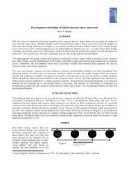
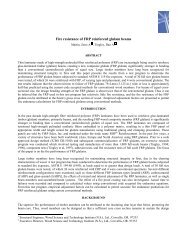
<strong>shear</strong> <strong>wall</strong> <strong>test</strong> samples in <strong>the</strong> City <strong>of</strong> <strong>Los</strong> <strong>Angeles</strong>-<strong>UC</strong>I <strong>program</strong>, <strong>the</strong> FME was estimated <strong>from</strong> <strong>the</strong> ‘backbone’ and<br />
‘degraded backbone’ curves as shown in Figure 1. The ‘backbone’ curve represents <strong>the</strong> envelope <strong>of</strong> peak loads for <strong>the</strong><br />
first cycle at a given displacement level whereas <strong>the</strong> ‘degraded backbone’ curve represents envelope <strong>of</strong> peak loads for <strong>the</strong><br />
last cycle at <strong>the</strong> same displacement level.<br />
City <strong>of</strong> LA - Shear Wall Tests<br />
8'x8' - 8d Hand Driven Common @ 6"/12" - 3/8" Str I<br />
8000<br />
7000<br />
7000<br />
6000<br />
6.5 %<br />
6733<br />
5000<br />
6500<br />
4000<br />
Backbone Curve<br />
6298<br />
Load (pounds)<br />
3000<br />
2000<br />
1000<br />
0<br />
-3.0 -2.5 -2.0 -1.5 -1.0 -0.5 0.0 0.5 1.0 1.5 2.0 2.5 3.0<br />
-1000<br />
-2000<br />
-3000<br />
Lateral Load (lbs)<br />
6000<br />
5500<br />
4.3 %<br />
5 %<br />
5883<br />
5815<br />
5589<br />
5565<br />
Degraded Backbone Curve<br />
-4000<br />
-5000<br />
5000<br />
-6000<br />
-7000<br />
-8000<br />
Displacement (inches)<br />
4669<br />
4528<br />
4500<br />
0.20 0.25 0.30 0.35 0.40 0.45 0.50<br />
Lateral Displacement (in)<br />
Figure 1 – Backbone & Degraded Backbone Curves for FME Calculation<br />
As a rule, each <strong>shear</strong> <strong>wall</strong> is deformed to successively higher displacement levels, and is cycled to each displacement<br />
level three times before <strong>the</strong> FME is reached and four times for deformations beyond <strong>the</strong> FME. Before <strong>the</strong> FME is reached<br />
<strong>the</strong>re is little difference in <strong>the</strong> force required to cycle <strong>the</strong> <strong>shear</strong> <strong>wall</strong> to a given displacement for each cycle. After <strong>the</strong><br />
FME is reached, however, <strong>the</strong> force required to cycle <strong>the</strong> <strong>shear</strong> <strong>wall</strong> to a given displacement <strong>the</strong> last time is somewhat less<br />
than <strong>the</strong> force required to deform <strong>the</strong> <strong>shear</strong> <strong>wall</strong> <strong>the</strong> first time.<br />
The definition adopted is that <strong>the</strong> Yield Limit State (YLS) or FME is reached when <strong>the</strong> force required to displace <strong>the</strong><br />
sample <strong>the</strong> last time is 95% <strong>of</strong> <strong>the</strong> force required to displace <strong>the</strong> sample to <strong>the</strong> same level as <strong>the</strong> first time. The YLS is <strong>the</strong><br />
point on <strong>the</strong> force-displacement diagram corresponding to <strong>the</strong> displacement and force reached on <strong>the</strong> first cycle to that<br />
displacement. Inasmuch as one <strong>of</strong> <strong>the</strong> relatively few data points that define <strong>the</strong> ‘degraded backbone’ curve (last excursion<br />
to a given displacement level) is likely to be exactly 95% <strong>of</strong> <strong>the</strong> ‘backbone’ curve (first excursion to a given displacement<br />
level), a parabolic curve fit process was adopted to determine <strong>the</strong> FME.<br />
Consider <strong>the</strong> data in Figure 1b that corresponds to <strong>the</strong> ‘windowed’ curves shown in Figure 1a. Assume that <strong>the</strong> ‘degraded<br />
backbone’ curve is 95.7% <strong>of</strong> <strong>the</strong> ‘backbone’ curve at a given displacement level whereas <strong>the</strong> ‘degraded backbone’ curve<br />
is 93.5% <strong>of</strong> <strong>the</strong> ‘backbone’ curve at <strong>the</strong> next highest displacement level. Clearly <strong>the</strong> ‘true’ FME lies between <strong>the</strong>se two<br />
pair <strong>of</strong> data points. By knowing <strong>the</strong> approximate FME level, one parabola is fit to three consecutive points on <strong>the</strong><br />
‘backbone’ curve (one point higher and two lower than <strong>the</strong> ‘true’ FME) and ano<strong>the</strong>r parabola is fit to <strong>the</strong> three<br />
consecutive points on <strong>the</strong> ‘degraded backbone’ curve. It is a relatively routine procedure to <strong>the</strong>n determine <strong>the</strong><br />
displacement level corresponding to <strong>the</strong> point where <strong>the</strong> ‘degraded backbone’ curve is 95% <strong>of</strong> <strong>the</strong> ‘backbone’ curve.
The point <strong>of</strong> maximum force reached during <strong>the</strong> <strong>test</strong> defines <strong>the</strong> Strength Limit State (SLS). The SLS occurs at <strong>the</strong><br />
maximum displacement for <strong>the</strong> maximum force attained. The force at <strong>the</strong> SLS need not be significantly higher than <strong>the</strong><br />
force at <strong>the</strong> YLS, but for a ductile element or sub-system <strong>the</strong> displacement at <strong>the</strong> SLS will be a significant multiple <strong>of</strong> <strong>the</strong><br />
displacement at <strong>the</strong> YLS. As noted earlier <strong>the</strong> YLS and SLS results are summarized in Tables 2 and 3.<br />
DESCRIPTION OF TEST CONFIGURATION AND PROCEDURE<br />
Test Program Characteristics<br />
As <strong>of</strong> January 2000, <strong>the</strong> City <strong>of</strong> <strong>Los</strong> <strong>Angeles</strong> – <strong>UC</strong> <strong>Irvine</strong> timber <strong>shear</strong> <strong>wall</strong> <strong>test</strong> has completed 27 <strong>of</strong> <strong>the</strong> proposed 35<br />
configurations. Three samples <strong>of</strong> each configuration were subjected to <strong>the</strong> SEAOSC <strong>test</strong> protocol for <strong>shear</strong> <strong>wall</strong>s. As a<br />
rule, <strong>the</strong> framing for <strong>the</strong> 27 configurations have been ‘similar’ in construction, however, <strong>the</strong> framing for <strong>the</strong> six groups<br />
that comprise this study were identical. Each frame consisted <strong>of</strong>: a) two – 4” x 4” posts, b) one – 3” x 4” sill, c) one – 3”<br />
x 4” center stud, d) two – 2” x 4” top plates, and e) four – 2” x 4” field studs. The hold-downs were specially designed<br />
and fabricated <strong>from</strong> heavy gauge, 3-inch structural channel.<br />
Test Setup<br />
The <strong>shear</strong> <strong>wall</strong> samples were attached to <strong>the</strong> base <strong>of</strong> <strong>the</strong> <strong>test</strong> fixture with four 5/8-inch diameter anchor bolts. The bottom<br />
plate <strong>of</strong> <strong>the</strong> <strong>shear</strong> <strong>wall</strong> was supported on a 3 ½-inch wide by 96-inch long steel rectangular bar. This bar was set such that<br />
it only supported <strong>the</strong> framing <strong>of</strong> <strong>the</strong> <strong>wall</strong>s. This allowed <strong>the</strong> sheathing panels to freely rotate when loading <strong>the</strong> <strong>shear</strong> <strong>wall</strong><br />
laterally without <strong>the</strong> panels bearing on <strong>the</strong> <strong>test</strong> fixture at <strong>the</strong> bottom.<br />
Anchor-bolt holes in <strong>the</strong> 3” x 4” sill were carefully located and pre-drilled using a drill jig to minimize bolt deformation<br />
and slip when <strong>the</strong> <strong>shear</strong> <strong>wall</strong> was laterally loaded in <strong>the</strong> plane <strong>of</strong> <strong>the</strong> <strong>wall</strong>. The diameters <strong>of</strong> <strong>the</strong> anchor-bolt holes in <strong>the</strong><br />
sill were limited to a maximum <strong>of</strong> 1/16-inch oversize. Square steel plate washers, 1/8-inch thick by 2½-inches square,<br />
were used under <strong>the</strong> bottom plate bolts.<br />
Racking <strong>shear</strong> loads were applied horizontally to <strong>the</strong> top <strong>of</strong> <strong>the</strong> <strong>shear</strong> <strong>wall</strong> <strong>test</strong> specimens through a steel H-beam lagscrewed<br />
(with 3/8-inch diameter lag screws spaced 6-inches on center) to <strong>the</strong> double top plate <strong>of</strong> <strong>the</strong> <strong>wall</strong>. The H-beam,<br />
in turn, was placed on a ¾-inch thick by 3-inch wide plywood spacer. The purpose <strong>of</strong> this spacer was to allow <strong>the</strong><br />
sheathing panels to rotate when <strong>the</strong> <strong>shear</strong> <strong>wall</strong> was loaded laterally, without bearing on <strong>the</strong> H-beam at <strong>the</strong> top corners <strong>of</strong><br />
<strong>the</strong> panels. The H-beam was restrained laterally (normal to <strong>the</strong> plane <strong>of</strong> <strong>the</strong> <strong>shear</strong> <strong>wall</strong>) by pairs <strong>of</strong> low-friction, Teflon<br />
pads fastened to <strong>the</strong> beam and to <strong>the</strong> adjacent steel bracing frames. This arrangement permitted in-plane displacement <strong>of</strong><br />
<strong>the</strong> <strong>wall</strong> during <strong>the</strong> <strong>test</strong> while preventing <strong>the</strong> top <strong>of</strong> <strong>the</strong> <strong>wall</strong> <strong>from</strong> twisting outside <strong>of</strong> <strong>the</strong> load-application plane.<br />
Racking <strong>shear</strong> loads were applied with a 55 kip capa<strong>city</strong>, <strong>program</strong>mable, double-acting hydraulic actuator (MTS Systems<br />
Corporation) that was bolted to a stiff vertical cantilever column hinged at <strong>the</strong> base to act as a lever arm. The hinged<br />
cantilever system was necessary to ‘multiply’ <strong>the</strong> actuator displacement, which was limited to 3-inches <strong>of</strong> stroke in <strong>the</strong><br />
push and pull directions, to achieve greater displacement at <strong>the</strong> top <strong>of</strong> <strong>the</strong> <strong>wall</strong>. The horizontal load at <strong>the</strong> top <strong>of</strong> <strong>the</strong> <strong>wall</strong><br />
was measured with a load cell in <strong>the</strong> horizontal plane <strong>of</strong> <strong>the</strong> top plate and steel H-beam.<br />
Instrumentation<br />
The seven data channels that were typically recorded during a <strong>shear</strong> <strong>wall</strong> <strong>test</strong> included <strong>the</strong> measurement <strong>of</strong> <strong>the</strong> -<br />
• Horizontal-load between <strong>the</strong> <strong>shear</strong> <strong>wall</strong> and <strong>the</strong> hinged cantilever column<br />
• Horizontal-displacement <strong>of</strong> <strong>the</strong> <strong>shear</strong> <strong>wall</strong> at <strong>the</strong> top plate<br />
• Horizontal-displacement <strong>of</strong> <strong>the</strong> bottom plate relative to <strong>the</strong> <strong>test</strong> fixture (lateral in-plane sliding)<br />
• Vertical-displacement at <strong>the</strong> bottom end <strong>of</strong> both end posts relative to <strong>the</strong> <strong>test</strong> fixture (uplift and compression)<br />
• Vertical-displacement <strong>of</strong> <strong>the</strong> hold-down connectors relative to <strong>the</strong> end posts (displacement/bolt slip)<br />
The horizontal load between <strong>the</strong> <strong>shear</strong> <strong>wall</strong> and <strong>the</strong> hinged cantilever column was measured with a Bonded Foil Type<br />
Strain Gage Load Cell, produced by Muse Measurements <strong>of</strong> San Dimas, CA. The load cell used for this <strong>test</strong> <strong>program</strong> was<br />
model SR-4-24K with a load rating <strong>of</strong> 24 kips @ 2.0024 mV/V.<br />
The horizontal displacement <strong>of</strong> <strong>the</strong> <strong>shear</strong> <strong>wall</strong> at <strong>the</strong> top plate was measured using a PSCC Rayelco Position Transducer,<br />
o<strong>the</strong>rwise known as a string potentiometer. Model P-20A (A246), having a position sensitivity <strong>of</strong> 51.01 mV/V/inch, was<br />
used for this <strong>test</strong> <strong>program</strong>. This voltage sensitivity corresponds to an accuracy <strong>of</strong> +/- 0.005 inch. The range <strong>of</strong> <strong>the</strong>
potentiometer was 0-20 inches. To account for <strong>the</strong> cyclic displacements <strong>of</strong> <strong>the</strong> <strong>test</strong> protocol, <strong>the</strong> potentiometer was set to<br />
a displacement <strong>of</strong> approximately 10 inches at <strong>the</strong> beginning <strong>of</strong> each <strong>test</strong>.<br />
The o<strong>the</strong>r five displacement measurements (sill slip, two post uplifts and two hold-down slips) were measured with<br />
Spring Return Linear / Position Sensor Modules (Precision Linear Potentiometers) produced by Duncan Electronics.<br />
Model 604 R4K potentiometers, having an accuracy <strong>of</strong> +/- 0.002 inches, were used to measure <strong>the</strong>se five displacements.<br />
Data Acquisition<br />
Data sampling for all <strong>shear</strong> <strong>wall</strong> <strong>test</strong>s was taken with <strong>the</strong> Strawberry Tree data acquisition system. This system includes<br />
several components including <strong>the</strong> Strawberry Tree Data Acquisition s<strong>of</strong>tware, <strong>the</strong> terminal panels, and <strong>the</strong> analog-todigital<br />
transition hardware. The terminal panels were a mechanism to attach <strong>the</strong> various instruments’ wiring to a more<br />
standard ribbon wire. This ribbon wire was, in turn, attached directly to <strong>the</strong> analog-to-digital boards within <strong>the</strong> computer<br />
system.<br />
Data was acquired at 50 Hz (one data point every 0.02 seconds). Each data value <strong>from</strong> each instrument was placed in a<br />
data-logging array in columnar format. Between 5,000 and 10,000 data points were recorded for each channel.<br />
COMPARISON OF SHEATHING RESULTS – OSB VS PLYWOOD<br />
The principal goal in <strong>test</strong>ing <strong>the</strong> six <strong>shear</strong> <strong>wall</strong> groups summarized in Table 4 was to observe <strong>the</strong> panel’s behavior due to<br />
different sheathing materials and nail densities. Three <strong>shear</strong> <strong>wall</strong>s were constructed for each <strong>of</strong> <strong>the</strong> following six<br />
configurations (listed as Groups 3, 4, 9, 11, 12 and 13) using hand-driven 10d common nails with a 1/2” edge distance on<br />
<strong>the</strong> sheathing:<br />
Table 4 – Shear Wall Configurations for OSB/Plywood Comparison<br />
G3 - 15/32” Str I plywood nailed at 6”/12” G11 – 15/32” OSB nailed at 6”/12”<br />
G4 - 15/32” Str I plywood nailed at 4”/12” G12 – 15/32” OSB nailed at 4”/12”<br />
G9 - 15/32” Str I plywood nailed at 2”/12” G13 – 15/32” OSB nailed at 2”/12”<br />
<strong>Results</strong> and Observations<br />
The strength and drift results for this collection <strong>of</strong> <strong>shear</strong> <strong>wall</strong> <strong>test</strong>s are summarized in Table 5. If <strong>the</strong> mean values are<br />
considered for each <strong>test</strong> group, <strong>the</strong>n <strong>the</strong> following observations can be made:<br />
Group<br />
Configuration Description<br />
Table 5 – YLS and SLS <strong>Results</strong> for OSB/Plywood Shear Walls<br />
YLS Averages<br />
SLS Averages<br />
Drift (%) Force (lbs) lbs/ft Drift (%) Force (lbs) lbs/ft<br />
3 15/32 STR I 6"/12" 0.26 3777 472 1.81 6748 843<br />
4 15/32 STR I 4"/12" 0.39 5451 681 1.97 9146 1143<br />
9 15/32 STR I 2"/12" 0.63 10124 1266 1.96 15177 1897<br />
11 15/32 OSB 6"/12" 0.19 2906 363 0.96 4461 558<br />
12 15/32 OSB 4"/12" 0.26 5579 697 1.40 8507 1063<br />
13 15/32 OSB 2"/12" 0.42 9672 1209 1.80 15274 1909<br />
• Nail density increases YLS nearly linearly<br />
6”/12” to 4”/12” (1.5x) increases YLS by 1.68x<br />
4”/12” to 2”/12” (2.0x) increases YLS by 1.80x<br />
6”/12” to 2”/12” (3.0x) increases YLS by 3.01x<br />
• Nail density increases SLS nearly linearly<br />
6”/12” to 4”/12” (1.5x) increases SLS by 1.63x<br />
4”/12” to 2”/12” (2.0x) increases SLS by 1.73x<br />
6”/12” to 2”/12” (3.0x) increases SLS by 2.84x
• For more densely nailed panels, OSB YLS nearly matches Plywood YLS (102%, 96%)<br />
• For more densely nailed panels, OSB SLS nearly matches Plywood SLS (93%, 101%)<br />
• For lightly nailed panels (6”/12”), OSB YLS is significantly lower than Plywood YLS (77%)<br />
• For lightly nailed panels (6”/12”), OSB SLS is significantly lower than Plywood SLS (66%)<br />
• Plywood drift capa<strong>city</strong> is relatively insensitive to panel nail density (1.80%, 1.96%, 1.97%)<br />
• OSB drift capa<strong>city</strong> is very sensitive to panel nail density (0.96%, 1.40%, 1.80%)<br />
Summary<br />
The experimental results to date <strong>from</strong> a <strong>test</strong> and analysis <strong>program</strong> have been reported. These results suggest that Plywood<br />
and OSB correlate well for more densely nailed panels, but for lightly nailed panels, OSB has significant strength<br />
reductions. OSB also tends to have lower drift capa<strong>city</strong> than similar plywood panels, with lightly nailed OSB panels<br />
having severe capa<strong>city</strong> reductions. Panels also tend to behave in a nearly linear fashion with regard to nail density.<br />
CONCLUSIONS<br />
Clearly reporting <strong>the</strong> results <strong>of</strong> a <strong>test</strong> <strong>program</strong> that has considered 27 different configurations is beyond <strong>the</strong> scope <strong>of</strong> one<br />
technical paper. While <strong>the</strong> comparison <strong>of</strong> six configurations with identical framing but different sheathing and nailing<br />
schedules has been presented, <strong>the</strong>re are many o<strong>the</strong>r comparisons that can (and will) be made during <strong>the</strong> final phase <strong>of</strong> <strong>the</strong><br />
<strong>test</strong> <strong>program</strong>. Stucco and gypsum <strong>wall</strong> board performance, light gage steel framing, OSB vs. plywood, perimeter and<br />
field nail density, stud spacing, center stud size, edge nailing distance, etc. are just some <strong>of</strong> <strong>the</strong> anticipated investigations.<br />
One study underway is <strong>the</strong> definition <strong>of</strong> <strong>the</strong> YLS and how its value is affected by using ‘degraded backbone curve value /<br />
backbone curve value’ ratios <strong>of</strong> 95% (<strong>the</strong> current standard) versus, say, 93% and 90% standards. Additionally, a YLS<br />
based solely on <strong>the</strong> backbone curve is being investigated. Despite <strong>the</strong>se ongoing studies, it may be <strong>of</strong> interest to report<br />
some recent (and preliminary) YLS/SLS observations <strong>of</strong> <strong>the</strong> data by APA [Rose, 2000]. The calculated <strong>the</strong> ratio <strong>of</strong> YLS<br />
to SLS <strong>from</strong> City <strong>of</strong> <strong>Los</strong> <strong>Angeles</strong> / <strong>UC</strong> <strong>Irvine</strong> data summaries given in Tables 2 and 3 provide <strong>the</strong> following observations<br />
<strong>of</strong> <strong>the</strong> YLS/SLS ratio:<br />
1. Wood structural panel sheathing/wood framing (17 sets, 51 <strong>test</strong>s) has an average value <strong>of</strong> 0.66 and is quite<br />
consistent. A value <strong>of</strong> 0.65 is suggested.<br />
2. Wood structural panel sheathing/steel framing (6 sets, 18 <strong>test</strong>s) is quite consistent and has an average value <strong>of</strong><br />
0.38 or 0.34 if one outlier (Group 16) is excluded. A value <strong>of</strong> 0.35 is suggested.<br />
3. Gypsum <strong>wall</strong>board/wood framing (2 sets, 6 <strong>test</strong>s) has an average value <strong>of</strong> 0.59. A value <strong>of</strong> 0.60 is suggested.<br />
4. Stucco/wood framing (2 sets, 6 <strong>test</strong>s) has an average value <strong>of</strong> 0.44 for <strong>the</strong> nailed configuration and an average<br />
value <strong>of</strong> 0.32 for <strong>the</strong> stapled configuration. A value <strong>of</strong> 0.45 is suggested for <strong>the</strong> nailed configuration whereas a<br />
value <strong>of</strong> 0.33 is suggested for <strong>the</strong> stapled configuration.<br />
REFERENCES<br />
1. Shepherd, R., 1996, “Standardized Experimental Testing Procedures for Low-Rise Structures”, Earthquake Spectra,<br />
EERI, Vol. 12, No. 1, pp 111-127.<br />
2. Porter, M.L., 1987, “Sequential Phased Displacement (SPD) Procedure for TCCMAR Testing”, Proceedings, 3rd<br />
Meeting <strong>of</strong> <strong>the</strong> Joint Technical Coordinating Committee on Masonry Research, US-Japan Coordinated Research<br />
Program, Tomanu, Japan.<br />
3. Rose, J. – APA, Tacoma, Washington, Private Communication, February 2000.