Annual Report 2000 - WIT
Annual Report 2000 - WIT Annual Report 2000 - WIT
80 0 Depth (m) 200 400 600 800 1000 -3000 -2000 -1000 0 1000 2000 3000 Distance (m) Figure 2: Earth model for a simple numerical experiment. Also shown is the ray family for a common-offset experiment with a source-receiver offset of 3000 m. below a homogeneous halfspace with an acoustic wave velocity of 6 km/s (see Figure 2). Below the interface, we consider a vertical fault at » ¿ 0 km, separating two homogeneous blocks with velocities of 5 km/s and 5.5 km/s on the left and right side of the fault, respectively. In this model, we have simulated an ensemble of commonoffset seismic surveys with source-receiver offsets ranging from 0 m to 4000 m. The reflection angle for the largest offset is about 68“ . A typical common-offset dataset (for a source-receiver offset of 3000 m) is depicted in Figure 3. The numerical model- 300 350 400 Time (ms) 450 500 550 600 650 700 750 800 -2000 -1500 -1000 -500 0 500 1000 1500 2000 Midpoint Coordinate (m) Figure 3: A numerically simulated common-offset dataset for the model in Figure 2.
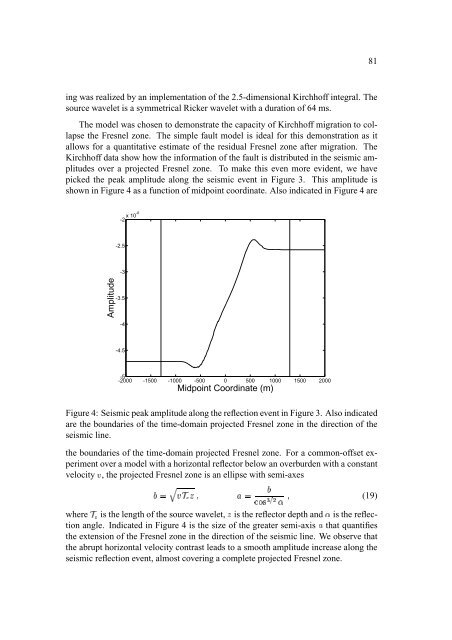
ê 81 ing was realized by an implementation of the 2.5-dimensional Kirchhoff integral. The source wavelet is a symmetrical Ricker wavelet with a duration of 64 ms. The model was chosen to demonstrate the capacity of Kirchhoff migration to collapse the Fresnel zone. The simple fault model is ideal for this demonstration as it allows for a quantitative estimate of the residual Fresnel zone after migration. The Kirchhoff data show how the information of the fault is distributed in the seismic amplitudes over a projected Fresnel zone. To make this even more evident, we have picked the peak amplitude along the seismic event in Figure 3. This amplitude is shown in Figure 4 as a function of midpoint coordinate. Also indicated in Figure 4 are -2 x 10⁻⁶ Midpoint Coordinate (m) -2.5 Amplitude -3 -3.5 -4 -4.5 -5 -2000 -1500 -1000 -500 0 500 1000 1500 2000 Figure 4: Seismic peak amplitude along the reflection event in Figure 3. Also indicated are the boundaries of the time-domain projected Fresnel zone in the direction of the seismic line. the boundaries of the time-domain projected Fresnel zone. For a common-offset experiment over a model with a horizontal reflector below an overburden with a constant velocity ê , the projected Fresnel zone is an ellipse with semi-axes â'’ ¼ (19) ¿ 7 ½X¼ * ¿ + + ì” ð ò íî³ï is the length of the source wavelet, is the reflector depth and ò is the reflec- ½ where tion angle. Indicated in Figure 4 is the size of the greater semi-axis that quantifies the extension of the Fresnel zone in the direction of the seismic line. We observe that the abrupt horizontal velocity contrast leads to a smooth amplitude increase along the * seismic reflection event, almost covering a complete projected Fresnel zone. â'’
- Page 41 and 42: · · v 0 B 0 £ & Ä Ã & v
- Page 43 and 44: 31 Dürbaum, H., 1954, Zur Bestimmu
- Page 45 and 46: Ã Ø Ì 0 0 Ì 4 0 Ã 0 G ' 4
- Page 47 and 48: Wave Inversion Technology, Report N
- Page 49 and 50: 0 0 ˜ ” Z ˜ ” Z 4 4
- Page 51 and 52: 39 strategy by combining global and
- Page 53 and 54: 41 elled data is presented in Figur
- Page 55 and 56: 43 0.2 Distance [m] 1000 1500 2000
- Page 57 and 58: 45 In Figure 10 we have the optimiz
- Page 59: 47 Gelchinsky, B., 1989, Homeomorph
- Page 62 and 63: § ¢ ø ø for a paraxial ray, ref
- Page 64 and 65: Œ § … Z ‹ Z § õ ø \ ø §
- Page 66 and 67: 54 As stated in Hubral and Krey, 19
- Page 68 and 69: § ó § 56 sequence. We made tes
- Page 70 and 71: 58 precision of the modeled input d
- Page 72 and 73: 60 Cohen, J., Hagin, F., and Bleist
- Page 75 and 76: Wave Inversion Technology, Report N
- Page 77 and 78: £ 65 The details of the theory inv
- Page 79 and 80: 67 of the figure. On both sides, a
- Page 81 and 82: 69 (a) (b) Depth (m) 600 800 Depth
- Page 83 and 84: 71 Langenberg, K., 1986, Applied in
- Page 85 and 86: È Û Ñ¿ = ¨ Í Ñ>* = ¿ + ð
- Page 87 and 88: Wave Inversion Technology, Report N
- Page 89 and 90: g ý g [ ^ â g [ g g g g g â h [
- Page 91: g § » ¹ [ƒŽ g 79 We now subst
- Page 95 and 96: ˆ 83 -0.05 -0.1 Amplitude -0.15 -0
- Page 97: 85 on a second-order approximation.
- Page 100 and 101: 88 kinematic (related to traveltime
- Page 102 and 103: ¨ º Ý È · § À · Á · Á ¼
- Page 104 and 105: ° ´ ´ ã ° ¼ ´ ´ þ Ò Ò ¥
- Page 106 and 107: 94 1 taper value ksi1 0 ksi2 Figure
- Page 108 and 109: 96 0 1 2 3 4 5 Depth [km] CMP [km]
- Page 110 and 111: 98 CONCLUSION As a generalization o
- Page 112 and 113: 100 weight during the stacking proc
- Page 114 and 115: 102 are not illuminated for every o
- Page 116 and 117: 104 obtained from Zoeppritz' equati
- Page 118 and 119: 106 PreSDM of Porous layer 0.358 re
- Page 120 and 121: 108 REFERENCES Gassmann, F., 1951,
- Page 122 and 123: 110 et al., 1992), Hanitzsch (1997)
- Page 124 and 125: 112 consecutive wavefronts). Howeve
- Page 126 and 127: 114 Numerical example We test the W
- Page 128 and 129: 116 Versteeg, R., and Grau, G., 199
- Page 130 and 131: 118 indicator. To extract elastic p
- Page 132 and 133: € b b 120 S where is the position
- Page 134 and 135: É É É É 122 The À constant (da
- Page 136 and 137: 124 0 Distance [ m ] 1000 2000 3000
- Page 138 and 139: 126 Kosloff, D., Sherwood, J., Kore
- Page 140 and 141: 128
ê<br />
81<br />
ing was realized by an implementation of the 2.5-dimensional Kirchhoff integral. The<br />
source wavelet is a symmetrical Ricker wavelet with a duration of 64 ms.<br />
The model was chosen to demonstrate the capacity of Kirchhoff migration to collapse<br />
the Fresnel zone. The simple fault model is ideal for this demonstration as it<br />
allows for a quantitative estimate of the residual Fresnel zone after migration. The<br />
Kirchhoff data show how the information of the fault is distributed in the seismic amplitudes<br />
over a projected Fresnel zone. To make this even more evident, we have<br />
picked the peak amplitude along the seismic event in Figure 3. This amplitude is<br />
shown in Figure 4 as a function of midpoint coordinate. Also indicated in Figure 4 are<br />
-2 x 10⁻⁶ Midpoint Coordinate (m)<br />
-2.5<br />
Amplitude<br />
-3<br />
-3.5<br />
-4<br />
-4.5<br />
-5<br />
-<strong>2000</strong> -1500 -1000 -500 0 500 1000 1500 <strong>2000</strong><br />
Figure 4: Seismic peak amplitude along the reflection event in Figure 3. Also indicated<br />
are the boundaries of the time-domain projected Fresnel zone in the direction of the<br />
seismic line.<br />
the boundaries of the time-domain projected Fresnel zone. For a common-offset experiment<br />
over a model with a horizontal reflector below an overburden with a constant<br />
velocity ê , the projected Fresnel zone is an ellipse with semi-axes<br />
â'’<br />
¼<br />
(19)<br />
¿ 7 ½X¼ * ¿ +<br />
+<br />
ì” ð ò íî³ï<br />
is the length of the source wavelet, is the reflector depth and ò is the reflec-<br />
½<br />
where<br />
tion angle. Indicated in Figure 4 is the size of the greater semi-axis that quantifies<br />
the extension of the Fresnel zone in the direction of the seismic line. We observe that<br />
the abrupt horizontal velocity contrast leads to a smooth amplitude increase along the<br />
*<br />
seismic reflection event, almost covering a complete projected Fresnel zone.<br />
â'’


