Annual Report 2000 - WIT
Annual Report 2000 - WIT Annual Report 2000 - WIT
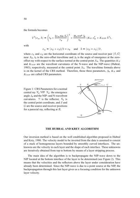
§ ¢ ø ø for a paraxial ray, reflecting at ô . - © ó ÿ ý ó § ó £ ø õ © ¢ ¢ ¤ 50 the formula becomes ÿ¡ ¦¨§ ý þ ü-ýþ1ÿ¡ ÿý £¥¤ ó© òó ó¥ £ ý ¤ © òó with and õ§ö©÷ near ù®ó , ÿ¡ þ1ÿ ÿ ¤ ÿ ¤ þ1ÿ ! where and are the horizontal coordinate of the source and receiver pair þ#" ¢%$ ÿ ÿ ó is the zero-offset traveltime and òó is the angle of emergence at the zerooffset ray with respect to the surface normal at the central ù®ó point . The quantities õ and õ§ö©÷ are the wavefront curvatures of the N-wave and the NIP-wave (Hubral, 1983), respectively, measured at the central ù®ó point . The traveltime formula above and are called CRS parameters. õ3ö©÷ is on the kernel of the CRS method. Therefore, those three parameters, òó , õ Figure 1: CRS Parameters for a normal central ray ù®ó'&)(+*Îù®ó : the emergence angle òó and the NIP- and N-wavefront curvatures. , is the reflector, ù®ó is the central point coordinate, and " and $ are the source and receiver positions 9 1 :;=@?BA7CEDGF HJIEKML / 021 :N>O?NA7CPD7F HJIEKEL . 35476 8 THE HUBRAL AND KREY ALGORITHM Our inversion method is based on the well established algorithm proposed in Hubral and Krey, 1980. The velocity model to be inverted from the data is assumed to consist of a stack of homogeneous layers bounded by smoothly curved interfaces. The unknowns are the velocity in each layer and the shape of each interface. These unknowns are iteratively obtained from top to bottom by means of a layer stripping process. The main idea of the algorithm is to backpropagate the NIP-wave down to the NIP located at the bottom interface of the layer to be determined (see Figure 2). This means that the velocities and the reflectors above the layer under consideration have already been determined. Since the NIP-wave is due to a point source at the NIP, the backpropagation through this last layer gives us a focusing condition for the unknown layer velocity.
k ilm § 51 0 X 0 v 0 Depth [km] 1 2 3 v 1 v 2 NIP 0 1 2 3 4 5 6 Distance [km] Figure 2: NIP-wavefront associated to the central zero-offset ray QSRUT'V7WXQSR , in red. To well describe the wavefront curvature along a ray path that propagates through the layered medium, we should consider two distinct situations: (a) the propagation occurs inside a homogeneous layer and (b) transmission occurs across an interface. Figure 3 depicts a ray that traverses the homogeneous Y -th layer (of velocity NZ ) being transmitted (refracted) at the interface Y[©]\ . Let us denote by ô_^a`Z the wavefront radius of curvature at the initial point of the ray (that is, just below the Y -th interface). The wavefront radius of curvature, ô¤öb`Zc5d , just before transmission, satisfies the relationship Z ¢ (1) NZgf ô-ö%`Zc5d ø±ô)^e`Z © ‚ iE„Nm xzy%{ uNv}|EsB~%uw nobp i r st%uvaw ‚ƒi hji xzy%{ uNv}|EsB~%uw_ € p ilm n¥q iPlm nobp ‚ƒilm Figure 3: Ray propagation through layer Y . where f § is the traveltime of the ray inside the layer. We now consider the change Z in wavefront curvature due to transmission at the interface. As shown in, e.g., Hubral
- Page 11 and 12: i TABLE OF CONTENTS Reviews: WIT Re
- Page 13 and 14: Wave Inversion Technology, Report N
- Page 15 and 16: 3 theory. It relates properties of
- Page 17: Imaging 5
- Page 20 and 21: 8 two hypothetical eigenwave experi
- Page 22 and 23: 7 ¢¥£§¦©¨ ; < calculate sear
- Page 24 and 25: 7 7 searches ¡ HNJOL for ¢IHNJML
- Page 26 and 27: 14 Trace no. 1000 1500 2000 0.5 1.0
- Page 28 and 29: 16 CDP number 3100 3000 2900 2800 2
- Page 30 and 31: 18 REFERENCES Höcht, G., de Bazela
- Page 32 and 33: 20 INVERSION BY MEANS OF CRS ATTRIB
- Page 34 and 35: 22 For synthetic data, it is easy t
- Page 36 and 37: — J J J J J J G J - J J G
- Page 39 and 40: Wave Inversion Technology, Report N
- Page 41 and 42: · · v 0 B 0 £ & Ä Ã & v
- Page 43 and 44: 31 Dürbaum, H., 1954, Zur Bestimmu
- Page 45 and 46: Ã Ø Ì 0 0 Ì 4 0 Ã 0 G ' 4
- Page 47 and 48: Wave Inversion Technology, Report N
- Page 49 and 50: 0 0 ˜ ” Z ˜ ” Z 4 4
- Page 51 and 52: 39 strategy by combining global and
- Page 53 and 54: 41 elled data is presented in Figur
- Page 55 and 56: 43 0.2 Distance [m] 1000 1500 2000
- Page 57 and 58: 45 In Figure 10 we have the optimiz
- Page 59: 47 Gelchinsky, B., 1989, Homeomorph
- Page 64 and 65: Œ § … Z ‹ Z § õ ø \ ø §
- Page 66 and 67: 54 As stated in Hubral and Krey, 19
- Page 68 and 69: § ó § 56 sequence. We made tes
- Page 70 and 71: 58 precision of the modeled input d
- Page 72 and 73: 60 Cohen, J., Hagin, F., and Bleist
- Page 75 and 76: Wave Inversion Technology, Report N
- Page 77 and 78: £ 65 The details of the theory inv
- Page 79 and 80: 67 of the figure. On both sides, a
- Page 81 and 82: 69 (a) (b) Depth (m) 600 800 Depth
- Page 83 and 84: 71 Langenberg, K., 1986, Applied in
- Page 85 and 86: È Û Ñ¿ = ¨ Í Ñ>* = ¿ + ð
- Page 87 and 88: Wave Inversion Technology, Report N
- Page 89 and 90: g ý g [ ^ â g [ g g g g g â h [
- Page 91 and 92: g § » ¹ [ƒŽ g 79 We now subst
- Page 93 and 94: ê 81 ing was realized by an implem
- Page 95 and 96: ˆ 83 -0.05 -0.1 Amplitude -0.15 -0
- Page 97: 85 on a second-order approximation.
- Page 100 and 101: 88 kinematic (related to traveltime
- Page 102 and 103: ¨ º Ý È · § À · Á · Á ¼
- Page 104 and 105: ° ´ ´ ã ° ¼ ´ ´ þ Ò Ò ¥
- Page 106 and 107: 94 1 taper value ksi1 0 ksi2 Figure
- Page 108 and 109: 96 0 1 2 3 4 5 Depth [km] CMP [km]
- Page 110 and 111: 98 CONCLUSION As a generalization o
§<br />
¢<br />
ø<br />
ø<br />
for a paraxial ray, reflecting at ô . -<br />
©<br />
ó<br />
<br />
ÿ<br />
ý<br />
ó<br />
§<br />
ó<br />
£<br />
ø<br />
õ<br />
©<br />
<br />
<br />
¢<br />
¢<br />
¤<br />
50<br />
the formula becomes<br />
ÿ¡ <br />
¦¨§<br />
ý<br />
þ<br />
ü-ýþ1ÿ¡<br />
ÿý<br />
£¥¤<br />
ó©<br />
òó<br />
ó¥<br />
£ ý ¤<br />
©<br />
òó<br />
with<br />
and<br />
õ§ö©÷<br />
near ù®ó ,<br />
ÿ¡<br />
þ1ÿ<br />
ÿ ¤<br />
ÿ ¤ þ1ÿ<br />
!<br />
where and are the horizontal coordinate of the source and receiver pair þ#" ¢%$<br />
ÿ ÿ<br />
ó is the zero-offset traveltime and òó is the angle of emergence at the zerooffset<br />
ray with respect to the surface normal at the central ù®ó point . The quantities õ<br />
and õ§ö©÷<br />
are the wavefront curvatures of the N-wave and the NIP-wave (Hubral,<br />
1983), respectively, measured at the central ù®ó point . The traveltime formula above<br />
and<br />
are called CRS parameters.<br />
õ3ö©÷<br />
is on the kernel of the CRS method. Therefore, those three parameters, òó , õ<br />
Figure 1: CRS Parameters for a normal<br />
central ray ù®ó'&)(+*Îù®ó : the emergence<br />
angle òó and the NIP- and N-wavefront<br />
curvatures. , is the reflector, ù®ó is<br />
the central point coordinate, and " and<br />
$ are the source and receiver positions<br />
9 1 :;=@?BA7CEDGF HJIEKML<br />
/<br />
021 :N>O?NA7CPD7F HJIEKEL<br />
.<br />
35476 8<br />
THE HUBRAL AND KREY ALGORITHM<br />
Our inversion method is based on the well established algorithm proposed in Hubral<br />
and Krey, 1980. The velocity model to be inverted from the data is assumed to consist<br />
of a stack of homogeneous layers bounded by smoothly curved interfaces. The unknowns<br />
are the velocity in each layer and the shape of each interface. These unknowns<br />
are iteratively obtained from top to bottom by means of a layer stripping process.<br />
The main idea of the algorithm is to backpropagate the NIP-wave down to the<br />
NIP located at the bottom interface of the layer to be determined (see Figure 2). This<br />
means that the velocities and the reflectors above the layer under consideration have<br />
already been determined. Since the NIP-wave is due to a point source at the NIP, the<br />
backpropagation through this last layer gives us a focusing condition for the unknown<br />
layer velocity.


