Annual Report 2000 - WIT

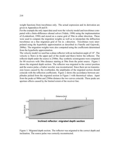
218
weight functions from traveltimes only. The actual expression and its derivation are
given in Appendices B and D.
For the example the only input data used were the velocity model and traveltimes computed
with a finite-difference eikonal solver (Vidale, 1990) using the implementation
of (Leidenfrost, 1998) and stored on a coarse grid of 50m in either direction. These
were used to compute the migration weights as well as to interpolate the diffraction
traveltimes on a fine migration grid of 5m in ¹ -direction. Traveltimes were interpolated
using the hyperbolic approximation as described in (Vanelle and Gajewski,
2000a). The migration weights were also computed using the coefficients determined
from the hyperbolic approximation.
The velocity model we used has a plane reflector with an inclination angle of 14º . The
velocity is 5km/s in the upper part of the model and 6km/s below the reflector. The
reflector depth under the source is 2500m. Ray synthetic seismograms were computed
for 80 receivers with 50m distance starting at 50m from the point source. Figure 1
shows the migrated depth section. The reflector was migrated to the correct position
and the source pulse, a Gabor wavelet, was reconstructed. Since there are no transmission
losses caused by the overburden, the amplitudes of the migrated section should
coincide with the reflection coefficients. Figure 2 shows the accordance between amplitudes
picked from the migrated section in Figure 1 with theoretical values. Apart
from the peaks at 900m and 2500m distance the two curves coincide. These peaks are
aperture effects caused by the limited extent of the receiver line.
1.5
Distance [km]
1 2 3
Depth [km]
2.0
2.5
Inclined reflector: migrated depth section
Figure 1: Migrated depth section. The reflector was migrated to the correct depth and
inclination. The source pulse was correctly reconstructed.