Annual Report 2000 - WIT

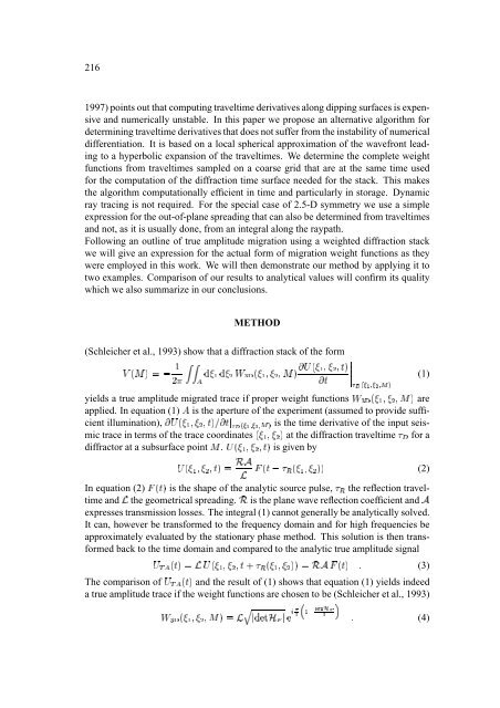
æVU ìÿå T
ü ýWYXZX[ 9\]9^\
Þ
_
Ý
Ý
Ý
Ý
Ý
Ý
Ý
ì
§Cb æ \] ê \
Ý
Ý
Ý
216
1997) points out that computing traveltime derivatives along dipping surfaces is expensive
and numerically unstable. In this paper we propose an alternative algorithm for
determining traveltime derivatives that does not suffer from the instability of numerical
differentiation. It is based on a local spherical approximation of the wavefront leading
to a hyperbolic expansion of the traveltimes. We determine the complete weight
functions from traveltimes sampled on a coarse grid that are at the same time used
for the computation of the diffraction time surface needed for the stack. This makes
the algorithm computationally efficient in time and particularly in storage. Dynamic
ray tracing is not required. For the special case of 2.5-D symmetry we use a simple
expression for the out-of-plane spreading that can also be determined from traveltimes
and not, as it is usually done, from an integral along the raypath.
Following an outline of true amplitude migration using a weighted diffraction stack
we will give an expression for the actual form of migration weight functions as they
were employed in this work. We will then demonstrate our method by applying it to
two examples. Comparison of our results to analytical values will confirm its quality
which we also summarize in our conclusions.
METHOD
(Schleicher et al., 1993) show that a diffraction stack of the form
êc ì
© dVeCfhgi ©©©©
gVj kml
(1)
ëa æ \] ê \
êOU
Ý`_
yields a true amplitude migrated trace if proper weight functions ëaöæ \] ê \ êOU ì
are
_
applied. In equation n (1) is the aperture of the experiment (assumed to provide sufficient
illumination), §Cb æ \] ê \
§ c
êNc ì @ § c & d¤eofpgi g¤j kml is the time derivative of the input seismic
trace in terms of the trace coordinates æ \] ê \ Ý
ì
at the diffraction traveltime òq for a
diffractor at a subsurface point U . b æ \] ê \
b æ \] ê \
êNc ì
is given by
(2)
êNc ìåsr!t
ì ì
u v æwc Þâòx æ \] ê \
In equation (2) v æwc ì
is the shape of the analytic source pulse, ò¨x the reflection traveltime
and the geometrical spreading. r is the plane wave reflection coefficient and t
expresses transmission losses. The integral (1) cannot generally be analytically solved.
It can, however be transformed to the frequency domain and for high frequencies be
u
approximately evaluated by the stationary phase method. This solution is then transformed
back to the time domain and compared to the analytic true amplitude signal
[ æ{c ìå u b æ \] ê \ êNcô bzy æ \] ê \ ì ìöå
r!t v æ{c ì
ò¨x
The comparison of
[ æwc ì
and the result of (1) shows that equation (1) yields indeed
bzy
a true amplitude trace if the weight functions are chosen to be (Schleicher et al., 1993)
(3)
Pƒ‚…„{†¦‡Gˆ
j "
(4)
¥j ]
ëa æ \] ê \
êOU ìöå u > & |~}/!€ & |