- Page 1 and 2:
Wave Inversion Technology WIT Annua
- Page 3:
Wave Inversion Technology WIT Wave
- Page 7:
Copyright c 2000 by Karlsruhe Unive
- Page 11 and 12:
i TABLE OF CONTENTS Reviews: WIT Re
- Page 13 and 14:
Wave Inversion Technology, Report N
- Page 15 and 16:
3 theory. It relates properties of
- Page 17:
Imaging 5
- Page 20 and 21:
8 two hypothetical eigenwave experi
- Page 22 and 23:
7 ¢¥£§¦©¨ ; < calculate sear
- Page 24 and 25:
7 7 searches ¡ HNJOL for ¢IHNJML
- Page 26 and 27:
14 Trace no. 1000 1500 2000 0.5 1.0
- Page 28 and 29:
16 CDP number 3100 3000 2900 2800 2
- Page 30 and 31:
18 REFERENCES Höcht, G., de Bazela
- Page 32 and 33:
20 INVERSION BY MEANS OF CRS ATTRIB
- Page 34 and 35:
22 For synthetic data, it is easy t
- Page 36 and 37:
— J J J J J J G J - J J G
- Page 39 and 40:
Wave Inversion Technology, Report N
- Page 41 and 42:
· · v 0 B 0 £ & Ä Ã & v
- Page 43 and 44:
31 Dürbaum, H., 1954, Zur Bestimmu
- Page 45 and 46:
Ã Ø Ì 0 0 Ì 4 0 à 0 G ' 4
- Page 47 and 48:
Wave Inversion Technology, Report N
- Page 49 and 50:
0 0 ˜ ” Z ˜ ” Z 4 4
- Page 51 and 52:
39 strategy by combining global and
- Page 53 and 54:
41 elled data is presented in Figur
- Page 55 and 56:
43 0.2 Distance [m] 1000 1500 2000
- Page 57 and 58:
45 In Figure 10 we have the optimiz
- Page 59:
47 Gelchinsky, B., 1989, Homeomorph
- Page 62 and 63:
§ ¢ ø ø for a paraxial ray, ref
- Page 64 and 65:
Œ § … Z ‹ Z § õ ø \ ø §
- Page 66 and 67:
54 As stated in Hubral and Krey, 19
- Page 68 and 69:
§ ó § 56 sequence. We made tes
- Page 70 and 71:
58 precision of the modeled input d
- Page 72 and 73:
60 Cohen, J., Hagin, F., and Bleist
- Page 75 and 76:
Wave Inversion Technology, Report N
- Page 77 and 78:
£ 65 The details of the theory inv
- Page 79 and 80:
67 of the figure. On both sides, a
- Page 81 and 82:
69 (a) (b) Depth (m) 600 800 Depth
- Page 83 and 84:
71 Langenberg, K., 1986, Applied in
- Page 85 and 86:
È Û Ñ¿ = ¨ Í Ñ>* = ¿ + ð
- Page 87 and 88:
Wave Inversion Technology, Report N
- Page 89 and 90:
g ý g [ ^ â g [ g g g g g â h [
- Page 91 and 92:
g § » ¹ [ƒŽ g 79 We now subst
- Page 93 and 94:
ê 81 ing was realized by an implem
- Page 95 and 96:
ˆ 83 -0.05 -0.1 Amplitude -0.15 -0
- Page 97:
85 on a second-order approximation.
- Page 100 and 101:
88 kinematic (related to traveltime
- Page 102 and 103:
¨ º Ý È · § À · Á · Á ¼
- Page 104 and 105:
° ´ ´ ã ° ¼ ´ ´ þ Ò Ò ¥
- Page 106 and 107:
94 1 taper value ksi1 0 ksi2 Figure
- Page 108 and 109:
96 0 1 2 3 4 5 Depth [km] CMP [km]
- Page 110 and 111:
98 CONCLUSION As a generalization o
- Page 112 and 113:
100 weight during the stacking proc
- Page 114 and 115:
102 are not illuminated for every o
- Page 116 and 117:
104 obtained from Zoeppritz' equati
- Page 118 and 119:
106 PreSDM of Porous layer 0.358 re
- Page 120 and 121:
108 REFERENCES Gassmann, F., 1951,
- Page 122 and 123:
110 et al., 1992), Hanitzsch (1997)
- Page 124 and 125:
112 consecutive wavefronts). Howeve
- Page 126 and 127:
114 Numerical example We test the W
- Page 128 and 129:
116 Versteeg, R., and Grau, G., 199
- Page 130 and 131:
118 indicator. To extract elastic p
- Page 132 and 133:
€ b b 120 S where is the position
- Page 134 and 135:
É É É É 122 The À constant (da
- Page 136 and 137:
124 0 Distance [ m ] 1000 2000 3000
- Page 138 and 139:
126 Kosloff, D., Sherwood, J., Kore
- Page 140 and 141:
128
- Page 142 and 143:
130 penetration distances and a pot
- Page 144 and 145:
and » ˆ Ö Ö is the scalar hydra
- Page 146 and 147:
Å éÙó ó ».-.‹œì/-j쨋
- Page 148 and 149:
136 TRIGGERING FRONTS IN HETEROGENE
- Page 150 and 151:
Ö ˆ Ö “P£'ˆ é ˆ ó,Lˆ¨
- Page 152 and 153:
Ö Ö Ê » Ø Ö » Ö Ê Ê Ê Ö
- Page 154 and 155:
142 300 250 200 a) eikonal equation
- Page 156 and 157:
144 Shapiro, S. A., and Müller, T.
- Page 158 and 159:
» i » m ×]Ú ‘Œƒšj'Ÿlk hM
- Page 160 and 161:
148 RESULTS Soultz-sous-Forêts Inv
- Page 162 and 163:
…„ƒ 150 for the smaller ellips
- Page 164 and 165:
152 Figure 5: The cloud of events f
- Page 166 and 167:
…„ƒ Î Î ÎÄÈ‹•¨ Î-È
- Page 168 and 169:
156 straightforward. The new approa
- Page 170 and 171: 158
- Page 172 and 173: 160 1982). There is also the so-cal
- Page 174 and 175: { ³ u ´ ´ ´ ´ -y ›-^œ ´ ´
- Page 176 and 177: Ï u u ¬ 164 To summarize, we deri
- Page 178 and 179: Ý ì á ä é å¤æDçzè ä é
- Page 180 and 181: ø M ã = ã Ù ø ä Ú ã Ù ø
- Page 182 and 183: ã Q c ã ä 170 a=10m; std.dev.=8%
- Page 184 and 185: 172 Frankel, A., and Clayton, R. W.
- Page 186 and 187: 174 It is well-known that inhomogen
- Page 188 and 189: ã ä ä ŸSŸ S ¡S¡ ©©¨¨ æ
- Page 190 and 191: Kneib, 1995 285-6000 superposition
- Page 192 and 193: 180 parameter: Hurst coefficient pa
- Page 194 and 195: 182 REFERENCES Bourbié, T., Coussy
- Page 196 and 197: 184 1999) in multiple fractured med
- Page 198 and 199: ‹œž Ÿ¢¡¤£¦¥ƒ§©¨ ‘
- Page 200 and 201: j jÆÅÇ[È”u j jÎÅÇ[È”uw
- Page 202 and 203: 190 Davis, P. M., and Knopoff, L.,
- Page 204 and 205: 192 properties from the measured se
- Page 206 and 207: 194 discussion of these problems ca
- Page 208 and 209: 196 Altogether, close to 260 shotpo
- Page 210 and 211: 198 Time (ms) 0 2 4 6 8 10 12 14 16
- Page 212 and 213: 200 of groundwater. ACKNOWLEDGEMENT
- Page 214 and 215: 202
- Page 216 and 217: 204 the wavefront curvature matrix
- Page 218 and 219: û ò é from ã äñ to ã î§ñ
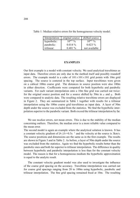
- Page 222 and 223: 210 Table 2: Median relative errors
- Page 224 and 225: 212 CONCLUSIONS We have presented a
- Page 226 and 227: 214 PUBLICATIONS Previous results c
- Page 228 and 229: æVU ìÿå T ü ýWYXZX[ 9\]9^\ Þ
- Page 230 and 231: 218 weight functions from traveltim
- Page 232 and 233: 220 REFERENCES Bleistein, N., 1986,
- Page 234 and 235: Š Ê ¦ Í ½ Í ’ » Ö ½ Ê
- Page 236 and 237: !¥”“Z• Ç ¤ ɨ§ — ‘
- Page 238 and 239: 226
- Page 240 and 241: 228 In this paper, we present a mor
- Page 242 and 243: L • MM+,ON N N Ž ú R N N N ú
- Page 244 and 245: 232 Figure 3: The evolution of a WF
- Page 246 and 247: 234 Let us analyze next the computa
- Page 248 and 249: 236 CONCLUSIONS We have presented a
- Page 250 and 251: 238
- Page 252 and 253: ’ Ç r 240 traveltimes, a computa
- Page 254 and 255: Ž Ž Ã Ž 242 Other two approxima
- Page 256 and 257: “ Ã Æ ³ 244 0 0.5 [km] 0 0.5 1
- Page 258 and 259: î r † Û(Û Ü Œ U Ú Ý Ü Û
- Page 260 and 261: 248 Ettrich, N., 1998, FD eikonal s
- Page 262 and 263: ø Ð ¡ Ð÷ö Ð'ø ú Ð ¡ Ð'
- Page 264 and 265: ø ü ø ø ý Þ do ø ý Ü
- Page 266 and 267: ø ö ø ú ü ö ü ¡ ü
- Page 268 and 269: ‹ 256 transport equation. Neverth
- Page 270 and 271:
258 tivalued geometrical spreading
- Page 272 and 273:
260 .
- Page 274 and 275:
262
- Page 276 and 277:
… " ¯ ü ý +- 4=° ü ü +
- Page 278 and 279:
ö ô æ º Ò x ¹ v ý ñ
- Page 280 and 281:
268 NUMERICAL RESULTS We constructe
- Page 282 and 283:
¹ õ ' ' -š' ù ¹ ù ' ' -š
- Page 284 and 285:
£ -š' - 272 Ô- —- Figure 6: C
- Page 286 and 287:
274 REFERENCES Aldridge, D. F. (199
- Page 288 and 289:
276
- Page 290 and 291:
278 3. 4. True-amplitude imaging, m
- Page 292 and 293:
280 Research Group Hamburg (Gajewsk
- Page 294 and 295:
282 Stefan Lüth Robert Patzig Refr
- Page 296 and 297:
284 Landmark Graphics Corp. 7409 S.
- Page 298 and 299:
286 TotalFinaElf Exploration UK plc
- Page 300 and 301:
288 as research assistant at Geoeco
- Page 302 and 303:
290 Ingo Koglin is a diploma studen
- Page 304 and 305:
292 Matthias Riede received his M.S
- Page 306 and 307:
294 Svetlana Soukina received her d
- Page 308:
296 Yonghai Zhang received the Mast