Annual Report 2000 - WIT
Annual Report 2000 - WIT Annual Report 2000 - WIT
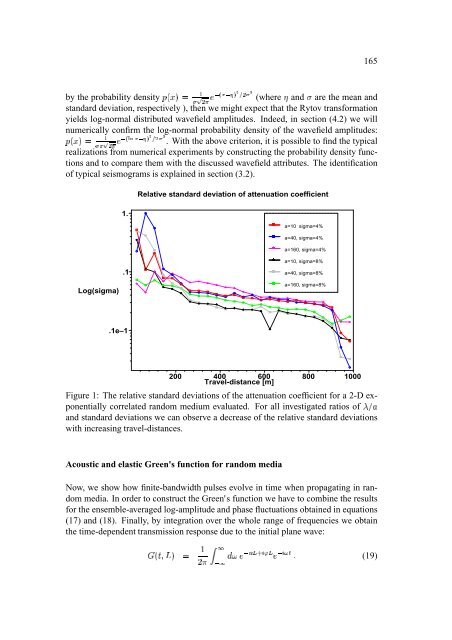
Ï u u ¬ 164 To summarize, we derived two pairs of wavefield ÏPŸ Ò ¼’¼ •¬ Ÿ Ò ¼©¿•Ð attributes, and •?® ¬¿® ä Ð , each of them related by (12). Therefore, the causality principle £ suggests to use the following logarithmic wavefield attributes in 2-D as well as 3-D {=Æ random media. £ • (17) ›¡œ ‘ ¬Lš Ò ¼’¼ ¬ Ÿn£·‘¿¬WŸ d {=Æ {=Æ { ‘ ® ¬¯®äA¬ÑŸ Ò ¼©¿ È (18) ›N®±œ Note that we used in equations (13)-(16) the 3-D wavefield attributes and that equations (17) and (18) are also valid for 2-D random media if we Ê skip in the integral RËÊ over and divide £ by . Self-averaging of the logarithmic wavefield attributes A self-averaged quantity tends to its mathematical expectation value provided that the wave has covered a sufficient large distance inside the medium. For 2-D and 3-D random media, we show that the attenuation coefficient { and the phase increment © in the above discussed approximations tend to their expectation values for increasing travel-distances. In analogy to the 1-D case, we compute the relative standard deviations of the attenuation coefficient and phase increment. Using synthetic wavefield registrations of finite-difference simulations (see section 3.1) we compute the relative Ÿ ¯ šéä«Ÿ £ { (éä Ÿ © ˆ ‘S©W¦éä standard deviation of the attenuation coefficient for several travel distances. Fig. (1) displays the numerically determined as a function of for 6 simulations is the center-frequency of the input wavelet, see also section 3.1). Instead of considering the relative phase increment fluctuations, we compute the relative traveltime fluctuations. This is an estimate of since . Again we observe the decrease of the relative standard deviation with increasing travel-distance (Fig. 2). It is clear that within the validity range of the Rytov approximation (that implies for finite travel-distances) only a partial self-averaging can be reached. That is to say the probability densities of the wavefield attributes have not yet converged to a 2 -function what would indicate that the quantities are not any more random. Therefore, it is expedient to look for the probability density of the logarithmic wavefield attributes and to introduce the concept of typical realizations of a stochastic process. Typical realizations are defined to be close to the most probable realization which is defined by the maximum of the probability density function (Lifshits et al., 1988, and Gredeskul and Freilikher, 1990). Now, the partial self-averaging means that we deal with wavefield realizations that are most likely to occur and therefore are typical realizations. It can be theoretically and experimentally shown ¡ that ® and are normally distributed random variables (see chapter (2.5) of Rytov et al., 1987). ¡ If is described
Ç Ç ä é å¤æDç¢è í 165 by the èšÊƒŸl‘ Ò4Ó probability ì Å Å@Õ "#Ö Ò I Ò Ö density (where and Ÿ are the mean and standard deviation, respectively ), then we might expect that the Rytov transformation Ò'Ô yields log-normal distributed wavefield amplitudes. Indeed, in section (4.2) we will w numerically confirm the log-normal probability density of the wavefield amplitudes: Ò Ó èšÊƒŸ ì Å ‡×
- Page 126 and 127: 114 Numerical example We test the W
- Page 128 and 129: 116 Versteeg, R., and Grau, G., 199
- Page 130 and 131: 118 indicator. To extract elastic p
- Page 132 and 133: € b b 120 S where is the position
- Page 134 and 135: É É É É 122 The À constant (da
- Page 136 and 137: 124 0 Distance [ m ] 1000 2000 3000
- Page 138 and 139: 126 Kosloff, D., Sherwood, J., Kore
- Page 140 and 141: 128
- Page 142 and 143: 130 penetration distances and a pot
- Page 144 and 145: and » ˆ Ö Ö is the scalar hydra
- Page 146 and 147: Å éÙó ó ».-.‹œì/-j쨋
- Page 148 and 149: 136 TRIGGERING FRONTS IN HETEROGENE
- Page 150 and 151: Ö ˆ Ö “P£'ˆ é ˆ ó,Lˆ¨
- Page 152 and 153: Ö Ö Ê » Ø Ö » Ö Ê Ê Ê Ö
- Page 154 and 155: 142 300 250 200 a) eikonal equation
- Page 156 and 157: 144 Shapiro, S. A., and Müller, T.
- Page 158 and 159: » i » m ×]Ú ‘Œƒšj'Ÿlk hM
- Page 160 and 161: 148 RESULTS Soultz-sous-Forêts Inv
- Page 162 and 163: …„ƒ 150 for the smaller ellips
- Page 164 and 165: 152 Figure 5: The cloud of events f
- Page 166 and 167: …„ƒ Î Î ÎÄÈ‹•¨ Î-È
- Page 168 and 169: 156 straightforward. The new approa
- Page 170 and 171: 158
- Page 172 and 173: 160 1982). There is also the so-cal
- Page 174 and 175: { ³ u ´ ´ ´ ´ -y ›-^œ ´ ´
- Page 178 and 179: Ý ì á ä é å¤æDçzè ä é
- Page 180 and 181: ø M ã = ã Ù ø ä Ú ã Ù ø
- Page 182 and 183: ã Q c ã ä 170 a=10m; std.dev.=8%
- Page 184 and 185: 172 Frankel, A., and Clayton, R. W.
- Page 186 and 187: 174 It is well-known that inhomogen
- Page 188 and 189: ã ä ä ŸSŸ S ¡S¡ ©©¨¨ æ
- Page 190 and 191: Kneib, 1995 285-6000 superposition
- Page 192 and 193: 180 parameter: Hurst coefficient pa
- Page 194 and 195: 182 REFERENCES Bourbié, T., Coussy
- Page 196 and 197: 184 1999) in multiple fractured med
- Page 198 and 199: ‹œž Ÿ¢¡¤£¦¥ƒ§©¨ ‘
- Page 200 and 201: j jÆÅÇ[È”u j jÎÅÇ[È”uw
- Page 202 and 203: 190 Davis, P. M., and Knopoff, L.,
- Page 204 and 205: 192 properties from the measured se
- Page 206 and 207: 194 discussion of these problems ca
- Page 208 and 209: 196 Altogether, close to 260 shotpo
- Page 210 and 211: 198 Time (ms) 0 2 4 6 8 10 12 14 16
- Page 212 and 213: 200 of groundwater. ACKNOWLEDGEMENT
- Page 214 and 215: 202
- Page 216 and 217: 204 the wavefront curvature matrix
- Page 218 and 219: û ò é from ã äñ to ã î§ñ
- Page 220 and 221: é 208 Table 1: Median relative err
- Page 222 and 223: 210 Table 2: Median relative errors
- Page 224 and 225: 212 CONCLUSIONS We have presented a
Ç<br />
<br />
Ç<br />
ä<br />
é<br />
å¤æDç¢è<br />
<br />
í<br />
165<br />
by the èšÊƒŸl‘ Ò4Ó<br />
probability ì Å Å@Õ<br />
"#Ö Ò<br />
I Ò<br />
Ö<br />
density (where and Ÿ are the mean and<br />
standard deviation, respectively ), then we might expect that the Rytov transformation<br />
Ò'Ô<br />
yields log-normal distributed wavefield amplitudes. Indeed, in section (4.2) we will<br />
w<br />
numerically confirm the log-normal probability density of the wavefield amplitudes:<br />
Ò Ó èšÊƒŸ ì Å ‡×


