Annual Report 2000 - WIT

105
Velocity [km/s]
6
5.5
5
4.5
4
3.5
3
velocities in saturated porous fault
Vp= 5.10 km/s
Porosity
range
25 % 35 %
2.5
Vs= 3.05 km/s
Vs= 2.85 km/s
2
0 0.1 0.2 0.3 0.4 0.5
porosity [ − ]
Vp
Vs
Vp= 4.80 km/s
0 0.4 0.8 1.2 1.6 2
Depth [km]
Time [s]
0 0.1 0.2 0.3 0.4 0.5 0.6 0.7
Shot Gather
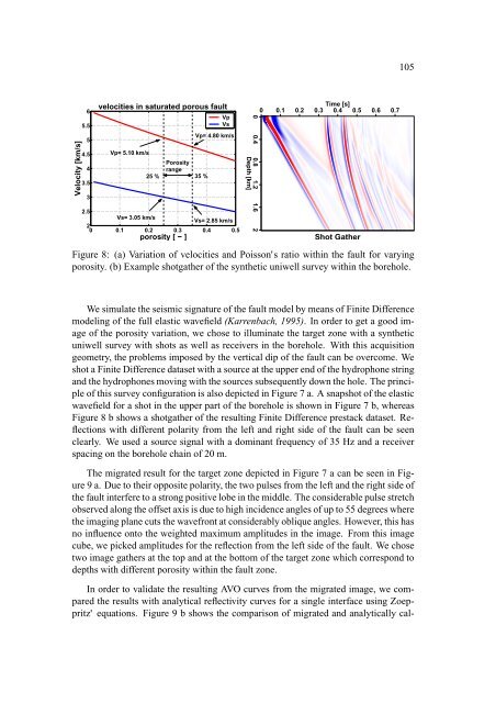
Figure 8: (a) Variation of velocities and Poisson's ratio within the fault for varying
porosity. (b) Example shotgather of the synthetic uniwell survey within the borehole.
We simulate the seismic signature of the fault model by means of Finite Difference
modeling of the full elastic wavefield (Karrenbach, 1995). In order to get a good image
of the porosity variation, we chose to illuminate the target zone with a synthetic
uniwell survey with shots as well as receivers in the borehole. With this acquisition
geometry, the problems imposed by the vertical dip of the fault can be overcome. We
shot a Finite Difference dataset with a source at the upper end of the hydrophone string
and the hydrophones moving with the sources subsequently down the hole. The principle
of this survey configuration is also depicted in Figure 7 a. A snapshot of the elastic
wavefield for a shot in the upper part of the borehole is shown in Figure 7 b, whereas
Figure 8 b shows a shotgather of the resulting Finite Difference prestack dataset. Reflections
with different polarity from the left and right side of the fault can be seen
clearly. We used a source signal with a dominant frequency of 35 Hz and a receiver
spacing on the borehole chain of 20 m.
The migrated result for the target zone depicted in Figure 7 a can be seen in Figure
9 a. Due to their opposite polarity, the two pulses from the left and the right side of
the fault interfere to a strong positive lobe in the middle. The considerable pulse stretch
observed along the offset axis is due to high incidence angles of up to 55 degrees where
the imaging plane cuts the wavefront at considerably oblique angles. However, this has
no influence onto the weighted maximum amplitudes in the image. From this image
cube, we picked amplitudes for the reflection from the left side of the fault. We chose
two image gathers at the top and at the bottom of the target zone which correspond to
depths with different porosity within the fault zone.
In order to validate the resulting AVO curves from the migrated image, we compared
the results with analytical reflectivity curves for a single interface using Zoeppritz'
equations. Figure 9 b shows the comparison of migrated and analytically cal-