TEACHER HANDBOOK LEAVING CERTIFICATE - Project Maths

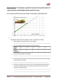
TEACHER HANDBOOK 

LEAVING CERTIFICATE 

HIGHER 

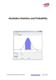
PROBABILITY & STATISTICS 

(Oct 2008 Syllabus)

Exploring concepts of probability and data analysis 

(Draft for October Syllabus 2008) 

Leaving Certificate Higher Level 

“When we are not sure, we are alive” 

Graham Greene 

Section 1: Suggested sequence of lessons 

Section 2: Notes and Terms 

Section 3: Appendices 

0.7 

f(x) 

0.6 

0.5 

0.4 

0.3 

0.2 

0.1 

0 

3 5 7 9 11 13 15 17 

x 

Draft 01 © Project Maths Development Team Page 2 of 66

0.3 

0.2 

0.1 

p 

1 2 3 4 5 6 7 8 9 10 11 12 13 14 15 16 17 

r 

Section 1: Suggested sequence of lessons 

LCH Strand 1 Statistics and Probability 

Prior Knowledge (for students who have not studied Project Maths for the Junior Cert) 

Collecting and recording data, tabulating data, drawing and interpreting bar charts, 

pie chart, trend graphs, discrete array expressed as a frequency table, drawing and 

interpreting histograms, mean and mode, mean of a grouped frequency distribution, 

cumulative frequency, ogive, median, interquartile range. 

Recurring themes in this section 

Recognising everyday examples of the use of statistics in relevant applications, 

evaluating reliability and quality of data and data sources, critically evaluating claims 

and inferences made based on statistics, drawing conclusions from graphical and 

numerical summaries of data, recognising assumptions and limitations, relevance of 

sample size 

Note 1: Items in square brackets refer to suitable reference document. 

e.g. [Census at school how to] refers to a document on the website, 

[Appendix 3 Conditional Probability] refers to Appendix 3 in this document 

Note 2: The CD icon 

is used throughout this document to indicate that there is a resource on 

the Student Disc, which is relevant to the topic in the title of the lesson. 


Lesson 1/Lesson 2 

Title: 

References: 

Content: 

Data Handling Cycle 

[Data Handling Cycle] document, [Census at school how to] document 

Complete Census at School (CAS) Questionnaire (possibly homework) 

www.censusatschool.ntu.ac.uk 

Complete Census at School (CAS) Questionnaire (possibly homework) 

www.censusatschool.ntu.ac.uk 

Data handling cycle (Pose a question, collect data, analyse data, interpret the result 

and revisit the original question to check if it was suitable) 

Primary and secondary sources of data 

Designing Questionnaires 

Analyse Census at School questionnaire 

(data types and suitable graphical representations, open/closed questions) 

Analyse spreadsheet from Census at School 

Types of data – category vs. ordered, discrete vs. continuous 

Match CAS data to data types. 

Using prior knowledge of graphical representations decide on suitable graphical 

representations for category vs. ordered data. Interpret data. Find the mode. 

(Bar charts and pie charts are suitable data representations for these types of data.) 

Time series data and trend graph e.g. met office data, temperature over period of 

time, points accumulated at end of season over a number of years. 

Lesson 3 

Title: 

References: 

Representing and interpreting data 

[Data Handling Cycle] document, 

[Limitations of measures of central tendency] document, 

[Let’s investigate] document, 

Single variable numeric data discrete v continuous, 

Content: 

(Ranking, range, tallying, grouping and use of different class intervals, 

frequency table) 

Mean, median and mode of raw data, grouping to facilitate calculation of these 

Mean of raw data v mean of grouped data 

Median identified after ranking and median identified from grouped data 


Mode identified 

Choice of suitable data representation - Discrete data – bar charts and pie charts 

Continuous data - histograms, frequency polygons, frequency curves 

Describe the distributions in terms of their shape, centre, and spread, and note any 

gaps and/or outliers. 

Subgroups of the class could work on different data, e.g. height, foot size, arm span 

from CAS. 

Lesson 4 

Title: 

Weighted mean 

References: 

Content: 

Weighted mean and applications 

Lessons 5, 6, 7 

Title: 

References: 

Stem Plots 

[Data Handling Cycle] document, [Spreadsheet practice] document, 

[Let’s investigate] document, 

Content: 

Stem Plots 

Lessons 8, 9, 10 

Students can use CAS data or generate their own data e.g. by guessing the number 

of sweets in a jar, the length of a line segment drawn on the board etc. 

For what types of data are stem plots suitable? 

One-sided, back-to-back 

Find median, range, maximum and minimum values, look for clustering of data, 

outliers. What are the advantages and disadvantages of stem plots? 

Title: 

Introduction to hypotheses testing and the Tukey quick test 

References: 

[Data Handling Cycle] document, [Tukey] document, 

Content: 

Sampling v Census, size of sample, randomness of sample 

Concept of hypothesis testing (Inferences made about populations based on 

samples) 

Null hypothesis H 0 , Alternate hypothesis H 1 

Tukey (Linked to back-to-back stem plot) 

Decision-making and Type 1 and Type 11 errors 


Lessons 11, 12 

Title: 

References: 

Content: 

Cumulative frequency 

[Let’s investigate] document 

Cumulative frequency polygon, cumulative frequency curve, quartiles, interquartile 

range, percentiles 


Title: 

Measures of dispersion 

References: 

Content: 

[Limitations of measures of central tendency] document, 

Measures of dispersion – Range then standard deviation and limitations thereof 

(effect of outliers) 

Lessons 15, 16, 17 

Shifting and rescaling data – adding or subtracting a constant and multiplying or 

dividing by a constant (see exercise on Student disc). 

Title: 

References: 

Paired data and correlation 

[Data Handling Cycle] document, [Correlation Coefficient] documents, 

[Appendix 1 Correlation coefficient by eye and by calculator], 

Content: 

Paired data, concept of correlation (positive, negative, strong, weak) scatter graph, 

line of best fit (by eye and by calculator), correlation coefficient (by calculator), 

correlation vs. causality, relevance of sample size 


Title: 

Fundamental Principle of Counting and permutations 

References: [Permutations and Combinations LCO] , 

Content: 

Fundamental Principle of Counting and permutations 

Lessons 20, 21, 22 

Title: 

References: 

Content: 

Combinations 

[Permutations and Combinations LCO] document 

Combinations 



Title: 

Introduction to probability 

Content: 


Language of probability, sample space(S), event, estimate likelihood of an event on a 

scale of 0% to 100%, 0 to 1, outcomes of simple random processes using practical 

experiments, listing all possible outcomes, relative frequency, probability as long 

term relative frequency 

The probability of an event E, 

number of times E occurs 

P( E) 

Lim 

n 

number of times the experiment is performed 

Title: 

References: 

Content: 

Using combinations to evaluate probabilities 

[Appendix 2 Probability and Statistics Practice Sheet 1] in this document 

How to use combinations to evaluate probabilities 


Title: 

Content: 

Axioms of probability 

Formally list rules/axioms of probability + complement +General Addition Rule 

Lesson 29 

Title: 

Content: 

Multiplication Rule 

Multiplication Rule for Independent events 


Lessons 30, 31, 32 

Title: 

References: 

Content: 

Investigating conditional probability 

[Appendix 3 Conditional Probability] in this document 

Conditional probability - Use of tables, tree diagrams, and set theory 

P( A and B) P( A 

B) 

P( B | A) 

 

P( A) P( A) 

Lead onto the General Multiplication Rule of probabilities, which does not require 

the events to be independent. 

P( A B) P( A) P( B | A) or 

P(A B)=P(B) P(A|B) (Either set may be called A or B). 

Formal definition of independence: A and B are independent if P( B | A) P( B) 


Title: 

Content: 

Consolidation of probability concepts 

Overview of probability using all rules and methods 

Lessons 35, 36, 37 

Title: 

References: 

Content: 

Bernoulli Trials 

[Binomial] T&L, [Appendix 4 Binomial Activity document] in this document 

Bernoulli Trials 


Title: 

References: 

Random variables and expected value 

[Expected Value notes NCCA] document, [Expected value activities] document, 

[Let’s investigate] document 

Content: 

Frequency distributions grouped and ungrouped represented by histograms, uniform 

distribution, Random variables, discrete and continuous which lead to discrete and 

continuous probability distributions 

Expected value E(X) of Probability distributions 



Title: 

References: 

Content: 

Binomial Distribution 

http://demonstrations.wolfram.com/BinomialDistribution/ 

Binomial Distribution as a discrete probability distribution 

The number of successes r from n trials is a random variable. 

Mean (expected value) of r and standard deviation for the binomial distribution, 

representing the binomial distribution graphically, r on the horizontal axis and P(r) 

on the vertical axis (Autograph) 

Lessons 42, 43, 44, 45 

Title: Normal Distribution and Standard Normal 

References: [Appendix 5], [Appendix 6] 

3 rules for success: 

1. Draw a diagram 



Content: 

Continuous Probability distributions – the Normal Distribution and the Standard 

Normal Distribution, probabilities of (or proportion of the population in) particular 

ranges in normal distributions using a standardising transformation 


Title: 

References: 

Normal approximation to the binomial distribution 

[See page 16 Notes and Terms section in this document] 

Content: Normal approximation to the binomial ( np 5, nq 5 ) 

Lessons 48, 49, 50 

Title: 

Sampling distribution of the mean 

References: [Appendix 7], [Appendix 8] 

Content: 

Sampling distribution of the mean, the role of the normal distribution, standard 

error of the mean 

 

x 


Title: 

Confidence intervals 

References: [Appendix 9] 

Content: 

95% confidence interval for population mean from a sample 


Lessons 53, 54, 55 

Title: 

Hypothesis testing 

References: single sample z –test http://en.wikipedia.org/wiki/Z-test , 

Hypothesis testing http://en.wikipedia.org/wiki/Hypothesis_testing 

Content: 

Hypothesis testing of specified population mean, hypothesis testing for binomial 

distributions using one- and two-tailed tests at a 5% level of significance, assuming a 

normal distribution applies. 

Types of hypothesis testing 

There are 3 types of hypothesis testing on the LCH course 

Population Mean 

(one sample z –test) 

1.96 z 1.96 

x 

 

 

n 

1 

1.96 1.96 

Hypothesis Testing 

Binomial Distribution 

1.96 z 1.96 

x 

1.96 1.96 

 

Tukey Quick Test 

Significance level 5% 1% 0.1% Significance level 

Critical value of tail - 7 10 13 Critical value of 

count 

tail - count 


Addition Rule (general addition rule) 

SECTION 2 NOTES AND TERMS 

For any 2 events E and F, the probability of E or F is 

P( E F) P( E) P( F) P( E F) 

. 

Bernoulli trial 

A Bernoulli trial is an experiment with only two possible outcomes, success and 

failure. If p is the probability of success then the probability of failure q = 1 – p. If the 

same Bernoulli trial is repeated n times in succession, then the probability of any set 

of outcomes can be obtained from the binomial expansion of (p + q) n . 

Binomial Experiment (Bernoulli experiment) – essential features of 

 

 

 

 

 

There are a fixed number of trials denoted by n 

The n trials are independent and are repeated under identical conditions 

Each trial has only 2 outcomes: success and failure 

For each trial, the probability of success (p) is the same. The probability of failure is 

denoted by q. Since each trial results in either success or failure , p + = 1 and q = 1-p 

In a binomial experiment we are trying to find the probability of r successes in n 

n 

r 

trials P( X r) 

p q 

r 

 

nr 

Binomial Probability Model 

A binomial probability model is appropriate for a random variable that counts the 

number of successes r in n (a fixed number) of Bernoulli trials. 

Binomial Probability Distribution 

When a Bernoulli trial is carried out n times, it gives a binomial probability 

distribution. The mean and the standard deviation of a binomial probability 

distribution are given by: 

np 

 

npq 

The binomial distribution is used when a researcher is interested in the occurrence 

of an event, not in its magnitude. For instance, in a clinical trial, a patient may 

survive or die. The researcher studies the number of survivors, and not how long the 

patient survives after treatment. 


Category type data - 

Category data -ordered 

Can be identified by names or categories and cannot be organised according to any 

natural order e.g. colour of hair, make of car, pets 

These are identified by categories which can be ordered in some way e.g. months of 

the year, days of the week, schoolwork pressure – a lot, some, a little, none 

Complement Rule (useful consequence of the Axioms of Probability) 

Conditional Probability 

P( E ') 1 P( E) 

Conditional probability is a probability that takes into account a given condition e.g. 

the probability of owning a games console given that you are between the ages 

12 – 25 (not the same as the probability of owning a games console.) P( B | A ) reads 

as the probability of B given A. 

P( A 

B) 

P( B | A) 

 

PA ( ) 

Correlation 

A statistical measure referring to the relationship between two random variables 

A positive correlation exists when each variable tends to increase or decrease as the 

other does, and a negative or inverse correlation if one tends to increase as the 

other decreases. 

Correlation Coefficient - 

A numerical value (between +1 and -1) which identifies the strength of the linear 

relationship between variables 

A value of +1 indicates an exact positive relationship, -1 indicates an exact inverse 

relationship, and 0 indicates no predictable relationship between the variables. 

Distribution 

The distribution of a variable gives the possible values of the variable and the 

relative frequency of each value. 

Distribution – uniform distribution 

A histogram which doesn’t appear to have any mode and in which all the bars are 

approximately the same height is said to be uniform. Hence, a distribution that is 

roughly flat is said to be uniform. 


Discrete Probability Distribution 

Expected Value 

If X is a discrete random variable, then for each possible value of X, i.e. X=x, we can 

work out the probability P(X = x) i.e. P(x). The set of all values of x with their 

associated probabilities is called a discrete probability distribution. 

The expected value of a random variable is its theoretical long – run average value. 

As it is an average value, it need not be a point of the sample space. 

E( X ) xP( x) 

 

Event (E) 

Histogram 

Independent Events 

The name given to an outcome or a particular set of outcomes when an experiment 

is conducted in probability 

A bar graph such that the area over each class interval is proportional to the relative 

frequency of data within this interval 

Two events are independent if the occurrence of one has no effect on the probability 

that the other will occur e.g. two rolls of a fair die. Two events A and B are 

independent if any one of the following is true 

P( A| B) P( A) 

P( B | A) P( B) 

P( A AND B) P( A) P( B) 


Measures of Central Tendency 

Mean 

Advantages: 

1. It is easy to define and understand 

2. It is easy to calculate 

3. It takes into account every value in the distribution 

4. It is often used for other statistical processing. e.g. 

standard deviation, comparing averages. The mean 

facilitates this type of further analysis better than the 

median 

5. It is used when sampling and can give reliable 

information about a population 

6. It is preferred to the median if the distribution is 

relatively even 

Disadvantages: 

1. If there are extreme values (outliers) in a distribution, 

it may give a distorted view of the distribution. 

2. It can give an unrealistic value for discrete data. E.g. 

average car passengers 3.2 

Median 

Advantages: 

1. It is more suitable than the mean 

if there are outliers. It gives a 

more accurate view of central 

tendency than the mean if there 

are extreme values. 

2. It is usually a value from within 

the distribution, as opposed to 

the mean which may not be a 

value within the distribution at all 

3. It is easy to identify, especially 

using a stem and leaf diagram 

Disadvantages: 

1. Difficult to use it in any further 

statistical processing 

2. It is not widely known nor used 

Multiplication Rule 

For independent events the probability that 

both A and B occur is 

P( A and B) P( A B) P( A) P( B) 

(General) Multiplication Rule 

P( A and B) P( AB) P( A) P( B | A) 

Mutually exclusive or disjoint events 

Numeric Data 

Mutually exclusive or disjoint events have no outcomes in common. They cannot 

occur at the same time/in a single outcome. They cannot both be the result of a 

single experiment e.g. when a card is removed from a deck of cards it cannot be 

both black and red (mutually exclusive) but it can be both black and a king (not 

mutually exclusive). 

Data represented by real numbers 

Numeric Data – continuous numeric data 

Data which can take assume an infinite number of values between any two given 

values e.g. height, arm span, foot length 


Numeric data – discrete numeric data 

Normal Distribution 

Normal Curve 

Data that can only have a finite number of numeric values e.g. the number of peas in 

a pod, age in years, and the number of persons in each household 

This is one of the most important continuous probability distributions. It was 

studied by De Moivre and Gauss and is sometimes called Gaussian. It turns up in 

very many real situations including nearly all measured physical characteristics of 

living things. It is very important not only because it can be applied to a wide variety 

of situations but also because other distributions tend to become normal under 

certain conditions. 

A normal curve is the graph of a normal distribution. It has a shape very like the 

cross section of a pile of dry sand. It is called a bell shaped curve because 

blacksmiths would sometimes use a pile of dry sand in the construction of the mould 

for a bell. 

About 68% of all values fall within 1 standard deviation of the mean, about 95% fall 

within 2 standard deviations of the mean and about 99.7% fall within 3 standard 

deviations of the mean. 

Normal Curve – characteristics of 

 

The curve is bell shaped with its highest point over the mean on the x – axis. 

It is symmetrical about a vertical line through . 

 

 

 

The curve approaches the horizontal axis but never touches it or crosses it 

The transition points between being concave upwards and concave downwards 

are at + and -. 

The parameters governing the shape of a normal curve are (locates the 

balance point) and (the extent of the spread) 


Normal Model as an approximation to a Binomial Model 

For a normal model to be a good approximation to a Binomial model, we must 

expect at least 5 successes and 5 failures i.e. np 5 and nq 5 . 

(i) np 5 

Stick graph of a Binomial distribution with n = 10 and p=0.2 written as B (10, 

0.2). The overall shape does not have the characteristics of a normal 

distribution. 

0.4 

p 

0.3 

0.2 

0.1 

r 

Figure 1 

(ii) 

−2 −1 1 2 3 4 5 6 7 8 9 10 

np 5 

“Stick graph” of a Binomial distribution with n = 16 and p=0.5 written as B (16, 0.5) 

(np = 8). Although it is a discrete distribution, its shape is very close to that of a 

normal. 

0.3 

p 

0.2 

0.1 

Figure 2 

1 2 3 4 5 6 7 8 9 10 11 12 13 14 15 16 17 

r 


Fitting a normal curve with the same mean and standard deviation as a binomial distribution to a 

binomial distribution 

Normal curve with mean = 8 and 

standard deviation =2 

0.3 

p 

“Stick graph” of a Binomial 

distribution B(16,0.5) i.e. mean 

np =8 and standard deviation 

0.2 

npq =2 

0.1 

r 

1 2 3 4 5 6 7 8 9 10 11 12 13 14 15 16 17 

Figure 3 

As n increases, the Binomial distribution becomes closer to a normal distribution 

0.1 

p 

0.08 

B(200,0.5) 

0.06 

0.04 

0.02 

20 40 60 80 100 120 140 160 180 200 

r 

Figure 4 

Normal as an appromimation to the Binomial – continuity correction 

As the normal distribution is a continuous distribution the binomial needs to be 

“made continuous” in order to compare it with the normal. We can do this by 

treating each individual x as an interval, from x - 0.5 to x + 0.5. Hence 8 becomes 

the interval 7.5 to 8.5. 

-0.5 and +0.5 are known as continuity corrections. 

In Figure 2 above, the stick whose height represents the probability of 8 successes in 

16 trials is replaced by a bar whose area represents this probability and the stick 

graph becomes a histogram when using the continuity correction. When using the 

normal distribution to approximate the binomial we are working out the area under 

the bars. 

As seen from figure 4, for large values of n this correction become negligible. In 

practice we only use a continuity correction for small n and if specifically asked. 


Outcome 

The outcome of a trial is the value measured or observed for an individual instance 

of that trial. 

Outcomes – discrete outcomes - 

All of the outcomes can be listed 

Outcomes – continuous outcomes 

Probability density function 

Probability Axioms 

There are an infinite number of outcomes and therefore they cannot be listed. 

Continuous probability distributions are commonly represented with a curve, 

y f ( x) 

called a probability density function, such that the area under the curve 

between a and b is equal to the probability that the outcome of the experiment is 

in the interval a x b . Since area under the curve is equal to probability, the 

total area under the curve is 1. 

See Appendix 5 on area under a normal curve using Autograph. 

1.0 P( E) 1, 

E S 

2. PS ( ) 1; P( )=0 

3. Addition Rule: P( E F) P( E) P( F) if E F= 

 

i.e E and F are mutually exclusive events. 

E 

F 

Random phenomenon: 

Random Variable 

We call a phenomenon random if we know what outcomes could occur but not what 

outcomes will occur. 

If all the possible outcomes of an experiment can be assigned different numeric 

values and we use a variable to label the outcomes, that variable is a random 

variable labelled X. We say that the quantitative variable X is a random variable 

because the value it takes on in an experiment is a random outcome. 

A particular value that X can have is denoted by the corresponding lower case letter 

x. 


Random Variable – Discrete 

If the random variable X can take on only distinct discrete values e.g. the number of 

heads I get when I toss 4 coins, then it is a discrete random variable. A discrete 

random variable gives rise to a discrete probability distribution. e.g. the binomial 

probability distribution 

Random Variable - continuous 

Sample Space(S) - 

Scatter plot 

If the random variable X can take on any real value in an interval, then X is a 

continuous random variable e.g. If x is the weight of a person chosen at random, 

then x is a continuous random variable. Continuous random variables lead to 

continuous probability distributions. 

The set of all possible outcomes when an experiment is conducted 

A graphical representation of the distribution of two random variables as a set of 

points whose coordinates represent their observed paired values 

Standard Deviation 

 

N 

 

i1 

( x ) 

i 

N 

2 

The standard deviation is the square root of the average squared deviations of the 

data values from the mean. Conceptually the standard deviation measures the 

“spread of the data”. A small standard deviation means that most data items are 

closely clustered about the mean while a large standard deviation means that the 

data items vary a lot from the mean. 

Probability 

density 

0.5 

0.4 

0.3 

0.2 

0.1 

f(x) 

Small 

Large 

For a normal distribution 

approximately 2/3 (68%) of the data 

lies within one standard deviation of 

the mean. 

−40 −30 −20 −10 10 20 30 40 50 

x 


Standard Normal Distribution 

Standard Units z 

This is the most frequently used normal distribution where the random variable is 

denoted z (standardised normal variable) and the mean = 0 and standard deviation 

= 1. (See standard units). 

As there are many different normal distributions with different means and standard 

deviations, and as their probability density functions are not integrable, we would 

need tables to work out 1 2 

P( x x x ). As it is not practical to have tables for 

every type of normal distribution we convert x values to z values i.e. standard units. 

z 

x 

 

Stem plots – advantages of 

When we standardize, we shift by the mean and rescale by the standard deviation. 

As the original mean was , when we take the mean of the data from every value 

the mean itself becomes zero. Shifting the data alone does not change the standard 

deviation. 

When we divide each of the shifted values by the standard deviation, the standard 

deviation is divided by as well and since it was to start with the new standard 

deviation becomes 1. A z score tells us how unusual a value is as it tells us how far 

away it is from the mean – the larger it is the more unusual it is. Any z score of 3 or 

more is rare and a z score of 6 or 7 is way out! 

 

 

 

 

 

A stem plot displays each separate data value 

Stem plots give a quick clear picture of the shape of a distribution and make 

it easy to identify clustering of data from the lengths of the branches. 

When the values on each branch are ordered, it is very easy to pick out the 

median, quartiles, max and min values and to identify any outliers. 

Stem plots can be used to display discrete or continuous type data 

Two data sets can be compared with a back-to-back stem plot. 

Stem plots - disadvantage of 

 

 

 

They are unsuitable for very large data sets 

Small data sets with a large range can be difficult to display on the same 

stem plot without rounding e.g. 432, 507,534,581,609,626,671,712,719. If 

these data points are rounded to 430, 500, 510,530, 580, 610,630,710,720 

they can easily be displayed with the hundreds digits as the stem and the 

tens digits as the leaves 

Stem plots cannot be used for category type data. 

Trial 

A single experiment in probability 


Sampling and Hypothesis Testing 

http://www.stats.gla.ac.uk/steps/glossary/hypothesis_testing.html#pvalue 

Census 

In a census, every member of the population is included. 

Population 

The entire group of individuals or instances about whom we hope to learn 

Sample 

Symbols used 

A sample is a subset of a population, from which we actually collect information in 

the hope of making inferences about the population, as most of the time the 

population mean and standard deviation are impossible to determine exactly. 

The sample should be representative of the population. 

Population parameters are written in Greek letters (e.g. for mean and for 

standard deviation, while sample statistics are written in Roman letters (e.g. x for 

mean and s for standard deviation). The mean of the sample means is written as 

x 

and the standard error of the distribution of the mean (see below) is written as 

 

x . 

Sample statistics 

These are numbers computed from a sample, such as sample size n, 

sample mean x , and sample standard deviation s. 

Sample Means –Distribution of Sample means 

If I take a random sample of 100 female students and measure their height – I would 

expect that the mean height of this sample would be equal to or very close to the 

mean height of the population of female students from which the sample was 

drawn. Another random sample of 100 students might give a different mean and 

again I would expect it to be close to the population mean. The means of all possible 

samples of size 100 would form a distribution of sample means, which would have 

its own mean and its own standard deviation , called the standard error of the 

x 

mean. 

http://www.censusatschool.org/international/rds/index.asp?country=&lang=en 

x 


Central Limit Theorem 

Let x denote the mean of a random sample of size n from a population having mean 

and standard deviation . 

 

x = mean of all the sample means of size n 

 

x = standard error of the mean 

Then 

 

 

 

x 

x 

 

 

 

n 

When the population is normally distributed, the distribution of the sample 

means is normal for any n. 

For 30 

regardless of the population distribution. 

n the distribution of the sample means, x is approximately normal 

Statistical Inference 

Inferring certain facts about a population from results found in a random sample 

from the population e.g. we may wish to draw conclusions about the heights of 

15,000 adult female students (the population) by examining only 100 students (a 

sample) from this population. 

Standard Error of the Mean 

 

x 

This is a good estimate of the standard deviation of the sample means, assuming 

that the sample is sufficiently large, n 30 . 

(Note standard error is not an “error” and it is not “standard” but it is a lot simpler to 

say than the “estimated standard deviation of the sample means”.) 

To convert sample means x in a normal distribution of sample means to standard normal z values 

use 

x x 

x 

z (one sample z – test) 

 

x 

n 


Sampling distributions of x and of x 

0.7 

f(x) 

0.6 

0.5 

0.4 

Probability distribution of sample 

means (n= 5) taken from the same 

population with 

x = =10.2 and 

1.4 

x 0.63 

n 5 

0.3 

0.2 

Probability distribution of random 

variable x taken for a population 

with =10.2 and = 1.4 

0.1 

x 

0 

3 5 7 9 11 13 15 17 

One of the graphs above represents the probability distribution of a random variable X, with mean 

=10.2 and = 1.4 

The second graph represents the distribution of the sample means from the same population. Since 

the original population is normally distributed, the distribution of the sample means is also normal. 

Then mean of the population and the mean of the sample means x 

are the same i.e. 10.2. The 

difference is in the standard deviation for x and x . The samples are of size n = 5, hence the standard 

deviation of the x distribution is much smaller than that of the population. This has the effect of 

squashing much more of the total probability into the region above the mean. 


95% Confidence interval for a population mean from a sample 

The interval in which the population mean will lie with 95% certainty, given a sample 

mean, the population standard deviation and the sample size n. If the population 

standard deviation is not known then the 1 sample standard deviation s may be used 

provided the sample size n is large. 

In the sampling distribution of the means 95% of all sample means lie within 1.96 

of the population mean as the sample means are normally distributed. 

 

x 

Normal Distribution of sample means 

-1.96 

 

x 

 

+1.96 

 

x 

1.96 z 1.96 

x 

 

 

1 

1.96 1.96 

x 

1.96 x 1.96 

x 

1 

x 

1.96 x x 1.96 and 

x 

1 1 

x 1.96 x 1.96 

1 x 1 

x 

x 

Hence the interval between 1 

x 1.96 x 1.96 

1 x 

1 

x 1.96 

x and x1 1.96 

x 

x 

will contain the population mean with 

95% certainty. This is known as the 95% confidence interval for the population mean. 

1 Calculating the sample standard deviation: Strictly speaking we should use n-1 instead of n in the denominator of the formula for s. 

s 

 

( x 

x) 

n 1 

2 

If n is large however this makes very little difference. 

http://www.stats.gla.ac.uk/steps/glossary/confidence_intervals.html#confinterval 


Statistical decisions 

Hypotheses 

Very often we wish to make a decision on a population based on a sample e.g. 

whether a new drug really works or whether one method of teaching a topic is 

better than another or whether a new machine is producing higher quality 

components than another one or whether one hair colour lasts longer than another. 

These decisions are called statistical decisions. 

In order to make statistical decisions it is useful to make some assumptions, which 

may or may not be true, about the populations. These assumptions are called 

hypotheses. We might assume that the new drug is no better than the old one (no 

change) or that both methods of teaching are equally effective (no difference) or 

that the new machine is no better than the old one or that the new hair colorant 

does not last any longer than the old one – such hypotheses as these are called null 

hypotheses. 

Null Hypothesis H 0 

Hypothesis Testing 

This is the term used for any hypothesis which is set up primarily for the purpose of 

seeing whether it can be rejected. Usually it is a statement of “no effect”, “no 

change”, “no difference”, other than that which would be caused by chance 

variations alone. We are assuming that the outcome is not “unusual”. If the null 

hypothesis cannot be rejected this does not mean that it is true beyond all doubt, 

but that under our method of testing it cannot be rejected. 

(Courtroom analogy – the defendant is initially assumed innocent – innocence is the 

null hypothesis) 

Hypothesis testing is the statistical method of testing the truth or otherwise of the 

null hypothesis. 

(Courtroom analogy – the trial) 

Alternative Hypothesis H 1 

This is the hypothesis to be accepted when the null hypothesis must be rejected. 

(Courtroom analogy – the defendant is guilty) 


Examples of null and alternative hypotheses 

H 0 : The new machine is the same as the old one - no change 

Depending on the decision we are asked to make then H 1 could be: 

H 1 : The new machine is better than the old one (gives rise to a one-tailed test -see 

below) 

H 1 : The new machine is worse than the old one (gives rise to a one-tailed test -see 

below) 

H 1 : The new machine is different from the old one (gives rise to a two-tailed test - 

see below) 

The level of significance of a hypothesis test 

This is the probability of rejecting H 0 when it is in fact true. 

(e.g. in a courtroom finding a defendant guilty when they are in fact innocent, or 

diagnosing a patient with a disease when they don’t actually have it) 

An outcome is said to be significant (“unusual”) at the 5% level of significance if the 

probability of it or a more unusual one occurring is less than 5%. 

Two tailed hypothesis test at a 5% level of significance 

Region of acceptance of the null 

hypothesis – it represents 95% of 

all results. 

Regions of rejection of the null 

hypothesis (0.025% of all results in 

each tail) 

0 

Reject the null hypothesis H 0 if z 1.96 or z 1.96 

-1.96 and 1.96 are the critical values of z for this test and the regions of rejection as 

shown are the critical regions. 


One tailed hypothesis test at a 5% level of significance 

(i) 

Right tailed test 

Reject the null hypothesis H 0 if z 1.645 

The entire critical region goes to one side of the distribution. 

0 

1.645 

The critical value of z for this test is z = 1.645 and the region of rejection is the critical 

region. 

(ii) 

Left tailed test 

-1.645 

0 

Reject the null hypothesis H 0 if z 1.645 

The critical value of z for this test is z = -1.645 and the region of rejection is the 

critical region. 

Deciding whether a test is one or two tailed is determined by the way the question 

is asked and not by the data. 

Phrases leading to two tailed tests 

 

 

 

 

“is different from” 

“is biased” 

“is fair” 

“is consistent with” 


Phrases leading to one-tailed tests 

 

 

 

 

 

“is better than” 

“is worse than” 

“is greater than” 

“is less than” 

“is biased towards” 

“helps to cure “ 

Key question we ask in hypothesis testing 

Could these data have happened by chance if the null hypothesis were true? If they 

were very unlikely to have occurred if the null hypothesis were true, this raises 

doubt about the null hypothesis. (Medical analogy – you would be very unlikely to 

have these symptoms if you were healthy (null hypothesis.) 

Procedure for a hypothesis test 

Type l error 

Type ll error 

P –value 

Write down the null hypothesis H 0 

Decide whether it’s a one tailed or a two tailed test, 

 

 

 

Specify the significance level and hence write down the critical value/values 

of z. (5% level of significance only required at L. C.) 

Convert the observed result into z - units. 

Reject the null hypothesis if z is in the critical region and accept the 

alternative hypothesis H 1 , else fail to reject H 0 . 

Rejecting the null hypothesis when it is in fact true 

(Courtroom analogy – finding the defendant guilty when they are in fact innocent, 

in medicine diagnosing a person with a disease (rejecting the null hypothesis that 

they are healthy) when they don’t in fact have the disease i.e. a false positive) 

Failing to reject the null hypothesis when it is in fact false 

(Courtroom analogy – finding the defendant innocent when they are in fact guilty, or 

in medicine diagnosing a person as healthy (accepting the null hypothesis that they 

are healthy) when in fact they have the disease i.e. a false negative.) 

The probability of finding data like these or even less likely, if the null hypothesis 

were true is the P-value. If the P-value is high these data are not unusual, they 

happen a lot, are consistent with the null hypothesis and we have no reason to 


eject the null hypothesis. (Medical analogy -you have a high probability of having 

these symptoms when you are healthy – the null hypothesis - so no reason to reject 

the assumption that you are healthy.) If the P-value is low then it means that these 

data would be very unlikely if the null hypothesis were true, so we are inclined to 

reject the null hypothesis but of course, we cannot be sure. 

Tukey quick test (compact form) 

Significance level 5% 1% 0.1% Significance level 

Critical value of 7 10 13 Critical value of 

tail - count 

tail - count 


Appendices 

Appendix 1: Correlation coefficient by calculator 

Appendix 2: Probability and Statistics Practice Sheet 1 

Appendix 3: Conditional probability 

Appendix 4: Binomial Activity 

Appendix 5: Investigate area under a normal curve using Autograph 

Appendix 6: Student activity on the normal distribution 

Answers to student activity on the normal distribution 

Appendix 7: Student activity to investigate the distribution of Sample Means 

Answers to Student activity to investigate the distribution of Sample 

Means 

Appendix 8: Using Autograph to investigate the distribution of Sample Means 

Appendix 9: Student Activity on confidence intervals 

Answers to student activity on confidence intervals 

Appendix 10: Files from Student Disc on Strand 1 JC and LC 


Appendix 1 

Correlation coefficient and equation of line of best fit using Casio fx-83ES, Natural Display 

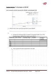
Input the following data on fat grams and total calories in fast food 

Total Fat (g) 

Total Calories 

1 Hamburger 9 260 

2 Cheeseburger 13 320 

3 Quarter Pounder 21 420 

4 Quarter Pounder with 30 530 

Cheese 

5 Big Mac 31 560 

6 Sandwich Special 31 550 

7 Sandwich Special with 34 590 

Bacon 

8 Crispy Chicken 25 500 

9 Fish Fillet 28 560 

10 Grilled Chicken 20 440 

11 Grilled Chicken Light 5 300 

1. Number each row of data if not already done to make it less likely to miss a row as data is 

being input into the calculator. 

2. MODE, 2(STAT ), 2(A+BX) 

3. Input the data into columns x and y.( Press = after inputting each data item) 

4. When they are all entered press SHIFT and 1(STAT) 

5. Choose 7( Reg i.e. regression) 

6. Choose 3 (r i.e. correlation coefficient), press = 

Gives correlation coefficient of 0 .9746 

To find the equation of the line of best fit y = A+Bx 

We are looking for the values of A (intercept on the y-axis) and B (slope of the line) from step 2 

above. 

1. The correlation coefficient, which has been calculated in Step 6 above, will have gone into 

row 12, column Y so it must be deleted, as it is not one of the original data items. Move the 

up arrow to row 12, column Y and press the DEL button. 

2. Press SHIFT, 1(STAT), 7(REG), 1(A) followed by = which gives A=193.85. (This appears in row 

12, column Y) 

3. The intercept, A, which has been calculated, will have gone into row 12 so it must be 

deleted, as it is not one of the original data items. Move the up arrow to row 12, column Y 

and press the DEL button. 

4. Press SHIFT, 1, 7, 2 followed by = which gives B = 11.731. This appears in row 12 column Y. 

The equation of the line of best fit is: y = 193.85+11.731x 


Appendix 2 

LCH Probability and Statistics 

Practice Sheet 1 

1) A bag contains 6 pens and 4 pencils. 2 items are drawn at random from the bag. 

What is the probability of getting: (a) 2 pens (b) 2 pencils (c) 1 pen and 1 pencil 

2) 2 cards are drawn at random from a pack of 52. What is the probability of getting: 

(a) 2 clubs (b) 2 red cards (c) 2 face cards (d) 2 aces 

3) A bag contains 7 red discs and 4 blue discs. Three discs are drawn at random. What is 

the probability of getting (a) 3 red discs (b) 3 blue discs (c) 2 red discs and 1 blue 

disc 

4) A person is dealt 5 cards from a pack of 52. (This is called a ‘hand’ in cards). What is 

the probability that this hand will be the 10, Jack, Queen, King and Ace of Hearts ? 

5) A person is dealt 5 cards from a pack of 52. 

(a)What is the probability that all of the 5 cards will be Diamonds? 

(b)What is the probability that none of the 5 cards is a Diamond? 

(Without using the P(S) = 1- P(F) rule) 

6) 25 women and 10 men attend a PTA meeting. At the meeting, a committee of 4 

people is formed to raise funds for the school. What is the probability that: (a) the 

committee is all female? (b) The committee is all male? (c) If the chairperson of 

the PTA (who is one of the 25 women) must be on the committee what is the 

probability that the committee will have a gender balance? (i.e. equal numbers of 

men and women) 

7) A bag contains five blue and six red discs. Three discs are drawn at random from the 

bag. Find the probability that at least one red disc is drawn. 

8) Verify the odds of winning each of the following combinations given in the box 

below. 


Appendix 3 

Conditional Probability 

U 

A bag contains 9 identical discs, numbered from 1 to 9. 

One disc is drawn from the bag. 

Let A = the event that ‘an odd number is drawn.’ 

Let B = the event that ‘a number less than 5 is drawn’ 

(i) 

(ii) 

What is (B|A)? 

Are the events A and B independent? 

A 

.5 

.7 

.9 

.1 

.3 

.2 

.4 

B 

.6 

.8 

(i) P(B|A) means the probability that the disc drawn is less than 5 given that it is odd. 

#( A 

B) Probability that the number is less than 5 and odd 2 

P( B | A) = = = 

# A 

Probability that the number is odd 5 

More generally we can 

say 

#( AB) P( AB) 

P( B | A) 

= 

# A P( 

A) 

2 

9 2 

= 5 5 

9 

(ii) No the events A and B are not independent. 

# B 4 

PB ( ) = # U 9 

2 

P( B | A) = 5 

Since P( B) P( B | A) the two events are not independent. 

i.e. the fact that the event A happened changed the probability of the event B happening. 


Appendix 4 

Binomial Activity 

Task 1: 

(a) If you were to roll a fair die 30 times how many times would you expect to get a 6? 

(b) Roll a die 30 times and record the results in the Table 1 below. 

Prediction __________ 

Table 1 

1 

Number 

which 

appears on 

die 

(outcome of 

trial) 

2 

How many 

times did this 

happen 

(It may be helpful to use 

tally marks) 

3 

Frequency 

4 

Relative 

Frequency 

5 

% of total scores 

6 

Success 

1, 2, 3, 4, 5 

Fail 

Totals 

Task 2: 

(a) If we call getting a 6 a “Success” and getting any other number a “Fail”, calculate the relative 

frequencies of success and failure and complete columns 4 and 5 in the table above. 

(b) Compare your prediction to the actual data recorded in Table 1. 


Task 3: 

(a) Fill in the Master Table below by recording and totalling the data collected by the other groups in 

the class. 

(b) Compare the relative frequencies from the Master Table below with those in the Table 1 above 

and comment on these with respect to your initial prediction. 

Master Table 

Task 4: 

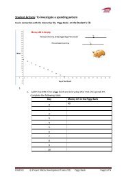
(a) The bar chart and corresponding table 2 below show the data recorded on a simulation of 

throwing a die 300 times. 

Using this data calculate the relative frequencies of success and failure as defined in Task 2(a) above. 

(b) Comment on the relative frequencies of success and failure, comparing these with those 

calculated using Table 1 above. 

Table 2 

1 2 3 4 5 6 


Appendix 5 

Investigate area under a normal curve using Autograph. 

Click on File, New 1D Statistics Page 

Click Data, Enter Probability Distribution 

Select Normal, OK 

Select = 0 and = 1 

Right click on the curve and select Probability Calculations 

Input lower and upper x – values to find the probability of finding x in a given 

interval. Read the probability on the task bar at the bottom of the screen 

Drag the yellow boxes to vary the limits 

0.5 

f(x) 

0.4 

0.3 

0.2 

0.1 

−3 Draft 01 −2 −1 © Project Maths Development 1 Team 2 Page 36 3of 66 

x

Appendix 6 

Student Activity on the Normal Distribution and Probability 

1. If the sales of a DVD in a store follow the normal distribution with mean of 300 and 

standard distribution of 50 

a) What is the probability that the sales on a certain day will be less than or equal to 

320? 

b) What is the probability that the number of sales on a certain day will be greater than 

or equal to 320? 

c) What is the probability that the number of sales on a certain day will be less than or 

equal to 280? 

d) What is the probability that the number of sales on a certain day will be between 

280 and 320 inclusive? 

e) What is the probability that the number of sales on a certain day will be between 

320 and 340? 

2) A certain type of battery has a life span that follows the normal distribution curve with a 

mean life of 180 hours and a standard deviation of 20 hours. 

a) What is the probability that a battery of this type selected at random will last more 

than 230 hours? 

b) What is the probability that a battery bought form this batch will last between 160 

and 200 hours inclusive? 

c) If 80% of the batteries last less than or equal to x hours, find the value of x. 

d) If 10% of these batteries last more than x hours, find the value of x. 

3) The time taken to undertake a particular task follows the normal distribution with a 

mean of 20 minutes and a standard deviation of 5 minutes. 

a) Estimate the probability that it takes 26 minutes or longer to complete the task. 

b) Estimate the probability that it takes less than or equal to 12 minutes. 

c) Estimate the probability that it takes between 17 and 24 minutes inclusive. 

4) A fair die is thrown 200 times, what is the probability that a 5 turns up 36 times or 

fewer? 

5) A coin is tossed 200 times, what is the probability of getting heads fewer than 80 

times? 


6) If 1000 copies of a particular newspaper advertising a competition were sold on a 

particular day and it is estimated that the probability of someone replying to the 

competition who buys the newspaper is ∙08. 

a) What is the probability of getting 65 or fewer entries? 

b) What is the probability of getting 85 or more entries? 

c) What is the probability of getting between 65 and 85 entries inclusive? 

7) The probability of apple in a batch being rotten is ∙02. If there are 10,000 in the batch, 

what is the expected number of rotten apples and what is the standard deviation? 

8) If 5% of a large consignment of apples are rotten and out of this consignment I select 

500 at random. What is the mean and standard deviation of the distribution of rotten 

apples in my sample? 

9) Among 10,000 random digits, find the probability that the digit 6 appears at most 950 

times. 

10) The weight of jam in a glass jar labelled 200g is normally distributed with mean 205g and 

standard deviation 10g. The weight of an empty glass jar is normally distributed with 

mean 250g and standard deviation of 5g. The weight of a glass jar is independent of the 

weight of the jam it contains. Find the probability that a randomly selected jar weighs 

less than or equal to 254 g and contains less than or equal to 202g jam. 


Answers for Student Activity on the Normal Distribution and 

Probability 

2. If the sales of a DVD in a store follow the normal distribution with mean of 300 and 

standard distribution of 50 

a) What is the probability that the sales on a certain day will be less than or equal to 

320? 

320-300 20 

Z= = = 4 

50 50 

Pr( x 320) Pr(z 4) 6554 

b) What is the probability that the number of sales on a certain day will be greater than 

or equal to 320? 

Pr(x 320)=Pr(z 4) 1 Pr(z 4)=1 6554= 3446 

c) What is the probability that the number of sales on a certain day will be less than or 

equal to 280? 

280-300 

Pr(x 280)=Pr(z )=Pr(z 4)=1 Pr(z 4) 

50 

=16554= 3446 

d) What is the probability that the number of sales on a certain day will be between 

280 and 320 inclusive? From above: 

Pr(280 x 320) 

Pr( x 320) 6554 

Pr( x 280) 3446 

Pr(280 x 320)= 6554 3446 3108 

e) What is the probability that the number of sales on a certain day will be between 

320 and 340? 

Pr(x 320)= 6554 

340 300 40 

Pr( x 340) Pr( z ) Pr( z ) Pr( z 8) 7881 

50 50 

Pr(320 x 340) 78816554= 1327 


11) A certain type of battery has a life span that follows the normal distribution curve with a 

mean life of 180 hours and a standard deviation of 20 hours. 

a) What is the probability that a battery of this type selected at random will last more 

than 230 hours? 

230 180 50 

Z 25 

20 20 

Pr( x 230) Pr( z 25) 1 Pr( z 2.5) 19938 0062 

b) What is the probability that a battery bought form this batch will last between 160 

and 200 hours inclusive? 

160 180 

For x 160 z= 1 

20 

Pr( x 160) Pr( z 1) 1 Pr( z 1) 18413 1587 

For x 200 

200-180 

Z= =1 

20 

Pr(x 200)=Pr(z 1)= 8413 

The probability of the battery lasting between 200 and 160 hours is 

8413 1587= 6828 . 

c) If 80% of the batteries last less than or equal to x hours, find the value of x. 

z 

Pr( z 

z ) 8 

1 

1 

84 84 

 

84 20 180 

x 

x 1968 

x 180 

20 

d) If 10% of these batteries last more than x hours, find the value of x. 

10% lasting more than x hours is the same as saying 90% last x hours or less. 

Pr( z z ) 0.9 

z 

1 

1 

128 

x 180 z 1 28 

20 

z 205.6 

Hence 10% of the batteries last more than 205.6 hours. 


12) The time taken to undertake a particular task follows the normal distribution with a 

mean of 20 minutes and a standard deviation of 5 minutes. 

a) Estimate the probability that it takes 26 minutes or longer to complete the task. 

26 20 

z 12 

5 

Pr( x 26) Pr( z 12) 1 Pr( z 1.2) 18894 1151 

b) Estimate the probability that it takes less than or equal to 12 minutes. 

12 20 8 

z 16 

5 5 

Pr( x 12) Pr( z 16) 1 Pr( z 16) 19452 0548 

c) Estimate the probability that it takes between 17 and 24 minutes inclusive. 

For 24 

24 20 

z= 8 

5 

Pr( x 24) Pr( z 8) 7881 

For x 17 

17 20 

z= 6 

5 

Pr( z 6) 1 Pr( z 6) 17257 2743 

Pr(17 x 24)= 7881- 2743= 5138 

13) A fair die is thrown 200 times, what is the probability that a 5 turns up 36 times or 

fewer? 

n 

1 5 

200 Pr(of a 5)=p= q=Pr(of not a 5)= 

6 6 

1 5 

np 200 5 nq=200 5 Hence binomial distribution 

6 6 

will approximate to the normal distribution. 

1 

=200 3333 

6 

1 5 

200 27.778 5.27 

6 6 

36 3333 

z 50664 

527 

Pr( x 36) Pr( z 5066) 6950 


14) A coin is tossed 200 times, what is the probability of getting heads fewer than 80 

times? 

1 1 1 

200( ) 100 = 200( )( ) 7 071 

2 2 2 

80 100 

z 2828 

7071 

Pr( z 2828) 1 Pr( z 2828) 199760 0024 

15) If a 1000 copies of a particular newspaper advertising a competition were sold on a 

particular day and it is estimated that the probability of someone replying to the 

competition who buys the newspaper is ∙08. 

a) What is the probability of getting 65 or fewer entries? 

p 08 

1000( 08) 80 = 1000( 08)( 92) 858 

65 80 

Z 17483 

858 

Pr( x 65) Pr( z 17483) 1 Pr( z 17483) 19599 04 

b) What is the probability of getting 85 or more entries? 

85 80 

z 5828 

858 

Pr( z 5828) 1 Pr( z 5828) 17190 281 

c) What is the probability of getting between 65 and 85 entries inclusive? 

Pr( x 85) Pr( x 65) 7190 04 679 

16) The probability of apple in a batch being rotten is ∙02. If there are 10,000 in the batch, 

what is the expected number of rotten apples and what is the standard deviation? 

Expected number =10,000(∙02) =200 

10000( 02)( 98) 14 


17) If 5% of a large consignment of apples are rotten and out of this consignment I select 

500 at random. What is the mean and standard deviation of the distribution of rotten 

apples in my sample? 

p 05 q= 95 

Mean =500( 05)=25 

Standard Deviation = 500( 05)( 95) 4873 

18) Among 10,000 random digits, find the probability that the digit 6 appears at most 950 

times. 

p 

1 9 

q= 

10 10 

1 1 9 

10000( ) 1000 = 10000( )( ) 900 30 

10 10 10 

950 1000 50 

z 167 

30 30 

Pr( x 950) Pr( z 167) 1 Pr( z 1.67) 19525 00475 

19) The weight of jam in a glass jar labelled 200g is normally distributed with mean 205g and 

standard deviation 10g. The weight of an empty glass jar is normally distributed with 

mean 250g and standard deviation of 5g. The weight of a glass jar is independent of the 

weight of the jam it contains. Find the probability that a randomly selected jar weighs 

less than or equal to 254 g and contains less than or equal to 202g jam. 

For more questions see 

254 250 

Pr( glass 254) Pr( z ) Pr( z 08) 7881 

5 

202 205 

Pr( jam 202) Pr( z ) Pr( z 03) 16179 3821 

10 

Pr( glass 254) and Pr( jam 202) 7881( 3821) 3011 

1. Questions on the normal and binomial distribution 

http://www.ltcconline.net/greenl/courses/201/probdist/NormalAreaBinomial.htm 

2. http://www.ltcconline.net/greenl/Courses/201/probdist/normal_distribution_and_c 

ontrol_.htm 

3. http://business.clayton.edu/arjomand/business/l6.html 

4. www.examinations.ie previous Leaving Cert Honours Option questions 

5. Ideas for questions http://www.intmath.com/Counting-probability/14_Normalprobability-distribution.php 


Appendix 7 

Student activity to establish the relationship between the mean of a 

population and the mean of the sample means and to investigate the 

distribution of sample means 

We are usually unable to collect information about a total population. The aim of sampling is to 

draw inferences about a population based on information obtained from a random sample taken 

from that population. We need to be able to interpret the information from the sample and state 

the degree of confidence we have in our results. 

Consider a population for which we can see the big picture i.e. a population of 100 fifteen year olds, 

whose heights in centimetres are given below in Figure 1. 

Figure 1 The heights of 100 fifteen year olds 

The mean of this population is = 164.7cm and the standard deviation is = 10.2. 

1) Write down the formulae for calculating mean and standard deviation. 

= _____________________ 

=_____________________ 

2) Verify the values given for the mean of the population and the standard deviation of the 

population using a calculator. 

= _____________________ 

=_____________________ 

The data in Figure 1 can be represented on a histogram with a class interval of 1, where the area of 

each rectangle represents the frequency of each data point and since the class interval is 1 the 

height represents the frequency. 


Figure 2: Histogram for the heights of a population of 100 fifteen year olds 

10 

f 

9 

8 

7 

6 

5 

4 

3 

2 

1 

x 

0 

130 135 140 145 150 155 160 165 170 175 180 185 190 195 200 

Questions and activities on the histogram in Figure 2 

1) Draw the frequency polygon. 

2) Are the heights normally distributed?________ 

3) Explain your answer_________________________________________________________ 

4) Draw a vertical line on the histogram, which indicates the mean of the histogram for the 

population. 

5) In which interval will the median lie? __________ 

6) What is the mode of the distribution? ___________ 

This is the big picture of the population. If we collected data from a sample of this population, 

would the sample reflect the population? Would different samples have a histogram looking the 

same as the histogram of the population? Would the samples have the same mean as the 

population? 

In order to get answers to these questions we take a large number of different samples (e.g. 100) 

from the list of heights in the table in Figure 3. 


The class divides into pairs. 

Each pair takes 10 random samples of 5 heights from the table of heights, Figure 3, which shows 

all the heights from Figure 1 but they are now numbered from 1 to 100. 

How to generate a random sample by using the random number generator 

RAND# on the calculator to generate random numbers from 1 to 100 

a. Shift, Setup, 2( LINEIO) 

b. Shift, Setup 6, Fix,0 

c. Shift, RAND#x100= 

d. Keep pressing = to generate random numbers from 1 to 100 

e. For each number generated record the item of data (height) associated with 

this number from Figure 3 into a table (Figure 4). 

f. Calculate the mean for each random sample of 5 heights. 


Figure 3: The heights of 100 fifteen yr olds numbered from 1 to 100 each height numbered to facilitate random sampling. 

(If number 41 comes up on the calculator the height associated with it is 176 cm) 

h/cm h/cm h/cm h/cm h/cm h/cm h/cm h/cm h/cm h/cm 

1 165 11 161 21 170 31 182 41 176 51 185 61 180 71 155 81 154 91 166 

2 165 12 152 22 174 32 167 42 165 52 171 62 172 72 150 82 181 92 165 

3 166 13 161 23 174 33 158 43 166 53 168 63 164 73 150 83 155 93 170 

4 168 14 144 24 164 34 154 44 177 54 173 64 178 74 158 84 165 94 175 

5 180 15 174 25 152 35 167 45 148 55 175 65 153 75 162 85 180 95 175 

6 157 16 172 26 155 36 140 46 147 56 160 66 152 76 166 86 168 96 158 

7 153 17 165 27 160 37 143 47 166 57 167 67 167 77 163 87 158 97 160 

8 150 18 157 28 172 38 167 48 184 58 172 68 165 78 159 88 158 98 177 

9 179 19 174 29 156 39 178 49 165 59 179 69 174 79 148 89 175 99 166 

10 157 20 159 30 163 40 165 50 162 60 153 70 145 80 170 90 176 100 180 


Figure 4: Table of 10 sets of 5 samples filled in by each pair of students 

Heights 

in 

Sample 

1 

Heights 

in 

Sample 

2 

Heights 

in 

Sample 

3 

Heights 

in 

Sample 

4 

heights 

in 

Sample 

5 

heights 

in 

Sample 

6 

heights 

in 

Sample 

7 

heights 

in 

Sample 

8 

heights 

in 

Sample 

9 

heights 

in 

Sample 

10 

Mean 

of each 

sample 

Using the 100 sample means collected from the full class the frequency table in Figure 5 can be filled 

in .The intervals used in the table are for one unit. For example, the interval labelled 165 includes all 

sample means x in the interval165 x 

166 . 

Figure 5 – Master table for Sample means of size n =5 

Class/cm Tally Frequency Class/cm Tally Frequency 

145 163 

146 164 

147 165 

148 166 

149 167 

150 168 

151 169 

152 170 

153 171 

154 172 

155 173 

156 174 

157 175 

158 176 

159 177 

160 178 

161 179 

162 180 

Sketch the histogram for the distribution of the 100 sample means of size n = 5 on figure 5. 

Figure 2 is shown first so that the distribution the heights can be compared with the distribution of 

the sample means of the heights. 


Distribution of heights for the population of 100 fifteen year olds. 

Figure 5 Distribution of the sample means (sample size n = 5) 

10 

f 

9 

8 

7 

6 

5 

4 

3 

2 

1 

0 

130 135 140 145 150 155 160 165 170 175 180 185 190 195 200 

x 

1) Compare the overall shape of the distribution of the sample means for n =5, with the shape of 

the distribution of the population heights. 

__________________________________________________________________________________ 

________________________________________________________ 

2) Calculate 

x 

(i) Compare the values of 

x 

 

x = ______________________ 

and 

 

x = _______________ = ____________ 

(ii) What do you notice about the mean of the sample means x 

and the mean of the 

population _______________________________________________________ 

3) Calculate the standard deviation of the sample means. 

(i) Standard deviation of the sample means = _____________ 


(ii) How does this compare with the standard deviation for the population distribution? 

____________________________________________________________________ 

Samples of size 5 are quite small but it would be very laborious to generate 100 random samples of a 

bigger size, for example 100 samples of size 20 each. However, the process would be the same as in 

the above exercise so we can use computer software to reduce the time factor as described in the 

following section. 


Using computer generated samples to investigate a distribution of sample means 

A computer program e.g. Autograph or Excel can be used to take any number of samples of different 

sizes from the data for a population. One such program, Autograph, was used to generate 100 

different random samples of 20 students from the original population of 100 students and calculate 

the mean of each sample. The sample means are shown below taken from the Statistics box in 

Autograph. 

See “Using Autograph to investigate the distribution of Sample Means” 

Figure 6 Frequency Table for the above results (100 samples of size 20) 

Sample mean x for n = 20 Frequency Cumulative frequency 

160 3 3 

161 4 7 

162 8 15 

163 21 36 

164 14 50 

165 18 68 

166 11 79 

167 13 92 

168 4 96 

169 4 100 

Sketch the histogram for the distribution of the 100 sample means of size n = 20 on figure 6. 

Figure 7 Distribution of the sample means (sample size n = 20) 

10 

f 

9 

8 

7 

6 

5 

4 

3 

2 

1 

0 

130 135 140 145 150 155 160 165 170 175 180 185 190 195 200 

x 

1) Compare the overall shape of the distribution of the sample means for n =20, with the shape 

of the distribution for n = 5 and with the distribution of the population heights. 

_____________________________________________________________________ 

_____________________________________________________________________ 

(ii) Compare the values of 

 

x and 

 

x = _______________ = _______ 

What do you notice about the mean of the sample means x 

and the mean of the 

population ? __________________________________________ 


2) Calculate the standard deviation of the sample means. 

(i) Standard deviation of the sample means = _____________ 

(ii) What is the approximate ratio of the standard deviation for the distribution 

of sample heights of size n = 20 heights compared with the standard 

deviation for the distribution of sample means of size n = 5? 

________________________________________ 

3) What would you expect if 100 different samples of 30 heights were taken? What would you 

predict about 

(i) The shape of the histogram representing the distribution of the sample 

means _____________________________________________________ 

(ii) The mean of the sample means _________________________ 

(iii) The standard deviation of the sample means ____________ _______ 

4) What effect is the size of the sample having on the mean of the sample means in relation to 

the mean of the population? 

__________________________________________________ 

5) What effect is the size of the sample having on the standard deviation of the sample means? 

_____________________________________________________ 

The standard deviation of the sample means can be estimated by the standard error of the 

mean 

x where 

x 

n 

6) Using the formula for standard error of the mean, calculate standard error of the mean for 

samples of size n = 40 and n = 50. 

for n 40 ______________ for n 50 ______________ 

x 

x 


We have seen that sample size affects the standard deviation (estimated by the standard 

error) of the distribution of sample means. 

Does the variation in standard deviation also depend on the number of samples taken? 

Graphs 1 to 6 show the distribution of sample means from a population using different sample 

sizes and different numbers of samples 

Graph 1: Histogram of the raw data from the population 

10 

f 

9 

8 

Graph 1: Graph of the raw data 

7 

6 

5 

N = 100 

Mean 164.72 

4 

3 

Standard deviation 10.21 

2 

1 

0 

135 145 155 165 175 185 195 

x 


Graphs 2 – 4 vary the number of samples while keeping the sample size constant. 

(Note the change in scale on the y –axis as more samples are taken) 

Graph 2: Histogram of 100 sample means from samples of size 30 

30 

f 

Graph 2: Graph of sample means 

100 samples 

20 

n = 30 

Mean 164.7 

10 


0 

135 145 155 165 175 185 195 

x 

Graph 3: Histogram of 500 sample means from samples of size 30 

200 

f 

180 

160 

140 


500 samples 

120 

100 

n = 30 

80 

60 

Mean 164.77 

40 

20 


x 

0 

135 145 155 165 175 185 195 

Graph 4 : Histogram of 1000 sample means from samples of size 30 

300 

f 

280 

260 

240 


220 

200 

180 

1000 samples 

160 

140 

120 

100 

80 

60 

40 

20 

0 

135 145 155 165 175 185 195 

x 

n = 30 

Mean 164.8 



Compare graph 5 with graph 3 – same number of samples but different sample sizes 


200 

f 

180 

160 

140 


500 samples 

120 

100 

80 

60 

40 

n = 50 

Mean 164.7 


20 

x 

0 

135 145 155 165 175 185 195 

Compare graph 6 with graph 4 – same number of samples but different sample sizes 


300 

f 

280 

260 

Graph 6 

240 

220 

200 

180 

160 

140 

120 

1000 samples 

n = 50 

Mean 164.7 

100 

80 

60 


40 

20 

0 

135 145 155 165 175 185 195 

x 

The other five graphs show distributions of sample means from the population. 

Comment on the 

(i) shapes of all the graphs 

(ii) The means of the distributions of the sample means compared to the mean 

of the population 

(iii) The standard deviations of the sample means 


Answers to questions on sample means 

N 

 

N 

 

2 

Xi 

( Xi 

) 

i1 i1 

1) = , where N = size of the population 

N 

N 

2) Use the calculator or Excel to find mean and standard deviation of the data. 

Questions and activities on the histogram in Figure 2 

1) Draw the frequency polygon. 

10 

f 

9 

8 

7 

6 

5 

4 

3 

2 

1 

x 

0 

130 135 140 145 150 155 160 165 170 175 180 185 190 195 200 

2) Are the heights normally distributed? No – but we are only looking at 100 heights 

3) The distribution is unimodal but is not symmetric about the mean 

4) 

5) In which interval will the median lie? 165 x 

166 

6) What is the mode of the distribution? 165 


Questions on the distribution of sample means n = 5 

Below is one possible set of results for 100 samples of size 5. 

Sample mean x for n = 5 Frequency Cumulative frequency 

154 1 1 

155 0 1 

156 1 2 

157 4 6 

158 2 8 

159 4 12 

160 5 17 

161 9 26 

162 4 30 

163 9 39 

164 12 51 

165 8 59 

166 3 62 

167 8 70 

168 10 80 

169 5 85 

170 4 89 

171 7 96 

172 3 99 

173 0 99 

174 1 100 

Histogram showing the distribution of the above 100 samples of size 5 

20 

f 

15 

10 

5 

0 

130 135 140 145 150 155 160 165 170 175 180 185 190 195 200 

x 

1) The overall shape for the distribution of sample means is more clustered than the distribution of 

the heights for the population. Hence the standard deviation is less. The distribution is also 

closer to a normal distribution. 

2) The mean of the sample means x 

165.2 is very close to the mean of the population 164.7 

3) Standard deviation of the sample means 

x = 4.275, much smaller than , the population 

standard deviation 


Answers to questions on the distribution of sample means 

Distribution of sample means of size n = 20 

1) This distribution of sample means of sample size 20 is approximately normal, with more 

clustering than the distribution for the population or for the distribution of sample means of 

size 5. 

2) x 

165 . This is approximately equal to the mean of the population 164.7 

3) 

(i)Standard deviation of the sample means x 

2.123 

(ii) The approximate ratio of the standard deviation for the distribution of sample heights of 

size n = 20 ( = 4.275) heights compared with the standard deviation for the distribution of 

x 

sample means of size n = 5( 

x 

2.123 ) is about 1:2. As n increased by 4, 

x decreased by 

about 2. 


7) What would you expect if 100 different samples of 30 heights were taken? What would you 

predict about 

i. The histogram would show tighter clustering about the mean than for 

sample sizes of 5 or sample sizes of 20. 

ii. The mean of the sample means will be approximately the same as the 

population mean 

iii. The standard deviation of the sample means will be less than for the 

standard deviation for a distribution of sample means of size 20. 

8) The mean of the sample means is approximately the same as the population mean and does 

not depend on the size of the sample provided the sample is large enough (see Central Limit 

Theorem). 

9) 

10.72 

 

x 

1.69 

n 40 

Comments on the graphs 1-6 

(i) The first graph is not normally distributed but the graphs of the sample means are all roughly 

normal ( n 30 for all). The first graph of the population shows far more variation and has a 

higher standard deviation than the graphs of the distributions of the sample means. 

(ii) All the means of the distributions of the sample means are approximately equal to the 

population mean. 

(iii) Graphs 2, 3 and 4 have approximately the same standard deviation and they all have the same 

sample sizes. 

Graphs 5 and 6 are very similar. They are more clustered around the mean than graphs 2, 3 and 

4, have larger sample sizes and smaller standard deviations. 

Hence the standard deviation seems to depend on the size of the sample and not on the 

number of samples taken. Also as the sample size increases the standard deviation decreases. 


Appendix 8 

Using Autograph to investigate the distribution of Sample Means 

Example: The data below shows the heights of a hundred 15-year-old students. 

1. Open an Autograph statistical page by clicking on the icon shown in Diagram 1. 

Statistic Icon 

Diagram 1 

2. From the Data dropdown menu select Enter Raw Data. Enter the data manually or paste from 

an Excel sheet. 

3. Group the data by pointing to Raw Data and right clicking. This will give you the option of 

grouping the data. Use class width = 1. 

4. Select the Histogram icon and the following will appear. 

5. Make sure that Frequency Density unit is 1. Click OK 

Change the axis by using Axis dropdown menu. 


6. Select the Histogram by clicking on it. Once it is selected Right Click and select Sample 

Means from the menu. The following box will should appear. 

7. Click on Single Sample and see what happens to the 

Histogram. A sample of 5 will be selected which are shown 

by 5 arrows pointing at the axis. The mean of this sample 

of 5 is shown by a small square on the axis. See diagram below. 

Info on Population and 

Sample. 

Data point 

8. Click on Clear Samples and the sample and the mean will disappear. Type in 20 for Sample 

Size and 30 for the number of samples and click on Sample. The following will appear. 

Info on Population and 

Sample. What can be 

deduced? 

Distribution of Sample Means 

9. If we now take a Sample Size of 30 (n = 30) and 100 samples. What can be deduced? Refer to the 

Central Limit Theorem. 


Appendix 9 

Student activity on confidence Intervals for the mean 

If we look at the distribution of 100 samples of 30 heights again, we see that it is approximately 

normal and would be perfectly normal if we took all possible samples of 30 heights. 

For the 100 samples of 30 heights, the population mean is 164.7(approximately equal to the 

mean of the sample means) and the standard error is 1.86. 

10.2 

x 1.86 

n 30 

30 

f 

20 

10 

0 

135 145 155 165 175 185 195 

x 

Listed below are the 100 samples of size 30 which gave rise to the above distribution 

164.1 168.3 163.7 165.1 164.1 163.1 163.7 163.7 164.3 165.3 

164.1 163.3 167.4 162.4 163.3 163.5 164.4 164.0 168.7 164.5 

165.2 165.7 165.0 164.1 166.2 163.9 161.2 161.4 162.6 163.9 

162.3 163.8 163.4 163.0 168.6 163.1 163.6 163.2 162.9 162.0 

164.3 164.1 162.1 163.9 166.1 164.0 166.8 162.1 162.8 165.2 

164.8 165.5 166.9 168.1 163.4 167.0 166.1 161.6 166.2 165.5 

165.8 164.4 166.3 162.9 160.1 160.4 165.8 165.6 165.5 164.1 

165.3 163.2 165.7 164.8 162.4 164.2 164.3 169.9 167.3 165.6 

166.8 163.7 166.2 166.2 165.0 169.6 167.9 167.7 166.4 164.9 

163.8 164.1 162.0 164.8 167.5 168.0 168.3 162.3 164.4 163.7 


Answer the following questions , applying the characteristics of normal distributions: 

1) What percentage of samples should fall within one standard error of the population mean? 

_________ 

2) What percentage of samples should fall within approximately two (1.96 to be more exact) 

standard errors of the of the population mean? 

_________ 

3) What heights represent the interval within approximately two (1.96) standard errors of the 

population mean? 

___________________________________ 

4) Using these values and the above 100 sample means, verify that the expected percentage of 

sample means falls within 1.96 standard errors of the population mean. 

5) What percentage of samples should fall within three standard errors of the of the population 

mean? _________ 

6) For each of the following sample means, taken from the above table, calculate an interval within 

1.96 standard errors of the mean. Does this interval contain the population mean? 

(i) x1 160.4 

(ii) x1 165.5 

7) We often wish to estimate a population mean based on the mean of one sample. Establish the 

95% confidence interval for the population mean using a single random sample of 30 heights 

with x 162.0 . 


Answers to questions on confidence intervals 

Q1 68% 

Q2 95% 

Q3. x 164.7 1.96(1.86) 168.34 and x 164.7 1.96(1.86) 161.05 

i.e. 161.05 x 

168.34 

Q4. 96% of the sample fall within 1.96 standard errors of the population mean which is reasonable 

as the distribution is not perfectly normal. 

Q5. 99.7% 

Q6. (i) 160.4+1.96(1.86) = 164.05 160.4 – 1.96(1.86) = 156.75 

The interval between 156.75 and 164.05 does not contain the population mean which is 

164.7. 

We expect 95% of samples to be within 1.96 x of the population mean and clearly not all 

samples have a mean within this interval. 

(ii) 165.5 +1.96(1.86) = 169.15 165.5-1.96(1.86) = 161.85 

The interval between 161.85 and 169.15 does contain the population mean. 

Q7. 162.0+1.96(1.86) =165.6 162.0-1.96(1.86) = 158.4 

We can say with 95% confidence that the interval from 158.4 to 165.6 contains the 

population mean. 

We expect that 95% of all sample means will be within 1.96 standard errors of the population 

mean. 


Appendix 10 

Files from Student’s Disc JC and LC 

Student Disc Leaving Certificate Strand 1 


Student Disc Junior Certificate Strand 1

TEACHER HANDBOOK LEAVING CERTIFICATE - Project Maths

Create successful ePaper yourself

Delete template?

Save as template?