Solutions for Homework #2

Solutions: Astronomy 540, Homework 2
Due: Wednesday, October 18 th , 2006
1. There are several ways to solve this problem; we give two here. The first is a rather
easy way where we use a formula that we know from introductory physics, the second is
more complicated but arises from first principles.
Solution a: We can use Kepler’s Third law of motion. We know that the orbit does not
depend on the eccentricity only on the semi-major axis. Let’s consider an orbital path,
with an eccentricity of 1, and with a semi-major axis of R/2. The infall time (the time a
body reaches the center) is the half of a full period:
The average density of the star is
t ff = t orb
2 = πR 3 2
2 √ 2GM
ρ =
3M
4R 3 π
Combining these we get the free fall time we were looking for:
t ff = 1 4
√
3π
2Gρ
(1)
(2)
(3)
For this derivation, we used the fact that the gravitational force inside a homogeneous
sphere only depends on the mass inside the central sphere, while the force from the outer
shells cancel out (the Homeoid Theorem).
Solution b: This solution gives the answer without any assumptions.
Let’s take a star, and let’s divide it up into a central part (M r ) and into the outer shell
(with mass: dm and width: dr). The equation of motion is
We can cancel out dm, and multiply by dr/dt
dm d2 r
dt 2 = −GM rdm
r 2 (4)
dr d 2 r
dt dt = −GM r dr
2 r 2 dt
(5)
The boundary conditions at t = 0 are: r = r 0 , ρ = ρ 0 , v = 0; or, dr/dt = 0 and
M r
= 4r 3 0 πρ 0/3. Multiplying equation (5) with dt, we get equation (6); and integrating
1

that, we get equation (7):
dr d 2 r
dt = −4πG
dt dt2 3r 2 r3 0 ρ 0dr (6)
( ) 2
1 dr
= 4πG
2 dt 3r r3 0ρ 0 + C 1 (7)
At r = r 0 (t = 0) we know that dr/dt = 0, so the constant of integration is
C 1 = − 4πG
3 r2 0 ρ 0 (8)
so this gives:
√
( )
dr 8πG
dt = 3 ρ 0r0
2 r0
r − 1
(9)
Let us use new parameters to make the derivation more simple. Let K be:
K =
√
8πG
3 ρ 0 (10)
and let θ be
θ = r r 0
(11)
This way
so dθr 0 = dr. The equation of motion then becomes:
Now let θ = cos 2 ξ. This way
dθ
dr = 1 r 0
(12)
dθ
dt = K √
1
θ − 1 (13)
dθ
dξ
The equation of motion then becomes:
= 2 sin ξ cos ξ (14)
2 sin ξ cos ξ dξ
dt
cos 2 ξ dξ
dt
√
1
= K
cos 2 ξ − 1 (15)
= K sin ξ
(16)
cos ξ
= K 2
(17)
2

After separating the variables and integrating, this comes to be
1
2 ξ − 1 4 sin(2ξ) = K 2 t + C 2 (18)
Looking at the boundary conditions (t = 0, r = r 0 ) we know that θ = 1 and cos 2 ξ = 1,
which means that ξ = 0. So that gives us C 2 = 0. At t = t ff , we know that r = 0, which
means that θ = 0, so ξ = π/2. So at the end of the infall
π
4 − 1 4 sin(π) = K 2 t ff (19)
so the free-fall time is:
If we substitute the value of K, we get:
t ff =
π
2K
(20)
t ff = 1 4
√
3π
2Gρ
(21)
For the Sun, this value is about 27 minutes.
2.a The distribution function gives the density distribution in a unit volume over velocities.
If we integrate the distribution function over velocities, we get the density at a certain
z position.
ρ(z) =
Substituting the distribution function, we get
∫ ∞
−∞
ρ(z) = ρ 0
√
2πσ
2
z
∫ ∞
−∞
fdv z (22)
e − Φ(z)+v2 z /2
σ 2 z dv z (23)
This can be rewritten as
ρ(z) = ρ 0
√
2πσ
2 z
∫ ∞
−∞
e − Φ(z)
σz
2 e − v2 z
2σz 2 dv z (24)
The first exponential part of the integral is a constant, so it can be brought out in front of
the integral. The second part is the well known Gaussian distribution with the 1/ √ 2πσ 2 z,
which integrated over −∞ to ∞ equals one. So we get
ρ(z) = ρ 0 e − Φ(z)
σ 2 z (25)
3

For an axisymmetric thin disk, the Poisson equation’s dependence from R cancels, and
we get
d 2 Φ(z)
dz 2
= 4πGρ(z) = 4πGρ 0 e − Φ(z)
σ 2 z (26)
Let’s convert this with the dimensionless units given in the problem. We know, that z =
ζz 0 . That gives
σ z
z = ζ √ (27)
8πGρ0
Let’s substitute this and the φ = Φ/σ 2 z
into the Poisson equation
d 2 (φσz 2)
d ( ) = 4πGρ
ζ 2 σz
2 0 e −φ (28)
8πGρ 0
The constants can be brought out of the derivative, and then we get the form we were
looking for:
2 ∂2 φ
∂ζ 2 = e−φ (29)
2.b It can be noticed, that this is a harmonic oscillator type of equation, so let’s multiply
both sides with the derivative of the value. We get
2 dφ d 2 φ
dζ dζ = dφ
2 dζ e−φ (30)
This is the same type of integral as was equation (6) in the first problem. Let’s integrate
the equation.
( ) 2
dφ
= −e −φ + c (31)
dζ
The integrational constant can be calculated if we know that the potential at the center of
the galactic plane is zero. That means that the gradient is also zero when ζ is zero. So we
get c = 1. We can take the square root of the equation and rearrange it.
dφ =
√
1 − e −φ dζ (32)
We will have to integrate this equation. Since the square root part is not to convenient,
let’s change variables, and arrange the equation so we have the same variables at the
same side. Let x = √ 1 − e −φ . That means that
dx =
e −φ
2 √ dφ (33)
1 − e−φ 4

dx = 1 − x2
dφ (34)
2x
2x
dφ = dx (35)
1 − x2 That changes our equation to be
By integrating that, we get
dζ = 2 dx (36)
1 − x2 ζ + const = 2 tanh −1 x (37)
Arranging that, and substituting x we get
tanh −1 (√
1 − e −φ )
= ζ + const
2
(38)
Taking the hyperbolic tangent of the equation we get
√
1 − e −φ = tanh
( ) ζ + const
2
(39)
>From the boundary conditions, we can see that the constant of integration is zero again.
So we get
( ) ζ
e −φ = 1 − tanh 2 (40)
2
Using tanh 2 + sech 2 = 1, we get
e −φ = sech 2 ( ζ
2
)
(41)
In the a part of the problem, we saw that e −φ = ρ(z)/ρ 0 . Substituting for that as well as
for ζ we get the equation given by Spitzer:
ρ(z) = ρ 0 sech 2 ( z
2z 0
)
(42)
3.a. The problem as given in Binney & Tremaine is a bit misleading, since if we use the
original Maxwellian distribution function given, we cannot derive the equation that we
are looking for. The original function given is
f 0 (v) =
ν 0
v2
(2πσ 2 e− 2σ
3/2 2 (43)
)
We know that this is a Gaussian distribution, with the particles’ energy in the exponential
5

part. Since our system also has a central mass (the black hole), the original Maxwellian
distribution function has to be modified, so that
E i = 1 2 v2 + V (44)
where
Our distribution function then is
V = − GM r
(45)
f 0 (v) =
ν 0
GM
e
(2πσ 2 3/2
)
rσ 2 − v2
2σ 2 (46)
The velocity distribution can be derived from
∫ vmax
ν(r) = 4π v 2 f 0 (v)dv (47)
v min
To calculate that, we have to know the boundary velocities. Since we are looking at "unbound"
particles, we know that the smallest allowable velocity is their "free" velocity,
√
which is v min = 2GM/r. The outer velocity boundary has to be ∞. Our starting equation
then becomes
By substituting our Maxwellian distribution, we get
∫ ∞√
ν(r) = 4π v 2 f 0 (v)dv (48)
2GM/r
∫
ν(r)
∞√
= 4π v 2 1 GM
e rσ
ν 0 2GM/r (2πσ 2 3/2 2 − v2
2σ 2 dv (49)
)
This equation is not straightforwardly solvable, but can be done using Mathematica,
which immediately gives the desired solution:
√ [ (√
ν(r) rH
= 2
ν 0 πr + rH er H/r
1 − erf
r
)]
(50)
3.b. To obtain the behavior at r ≪ r H , we use equation (1C-13) from Binney & Tremaine
which says:
e−x2
lim (1 − erf x) = √ . (51)
x→∞ πx
6

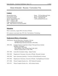
We can use this to approximate the second term for r → 0, which yields
√
ν(r) rH
≈ 2
ν 0 πr + e er H/r
−r H/r
√ π
√r H /r . (52)
>From this it is straightforward to see that the second term goes to zero as r → 0. This
can also be seen by plotting the function, as shown in Figure 1.
1
exp(1/x)*(1-erf(sqrt(1/x)))
0.9
0.8
0.7
0.6
0.5
0.4
0.3
0.2
0.1
0
-10 -5 0 5 10
Figure 1: The second part of the density function
Hence the density profile at r ≪ r H is
√
ν(r) rH
= 2
ν 0 πr
(53)
or
ν(r) ∝ r −1/2 (54)
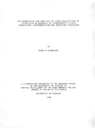
4. To solve this problem, we have to make a few assumptions. The first, and most important
one, is that the Cluster Formation Rate (CFR) was constant throughout the lifetime
of the Galaxy. The data plot can be seen in Figure 2.
An equation can be fitted to the points
N = N 0 10 −ta , (55)
where N 0 is an initial number density, t is the elapsed time, and a is a constant. The data
points are fit with N 0 = 78 and a = 0.5.
To estimate the number of stars from dispersed clusters, we need to compute the
difference between the number of clusters observed in a time interval as compared to
7

100
10
N clust [1/(kpc 2 Gyr)]
1
0.1
0.001 0.01 0.1 1 10
age [Gyr]
Figure 2: The fitted curve to the number density of clusters
the number of clusters that formed (ie., compute the area between a horizonatal line at
78clusters/kpc 2 /Gyr and the fit to the data points). This yields
N disp = 766 clusters
kpc 2
∗
x1000
cluster
(56)
Converted to the number of stars per square parsec,
If we distribute this into a 100pc thick layer, we get
The stellar number density in the Solar neighborhood is
ρ stars = .7665 ∗
pc 2 (57)
ρ stars = 0.007662 ∗
pc 3 (58)
ρ stars ∼ 0.14 ∗
pc 3 (59)
Which means that about 5% of the stars in the solar neighborhood have been formed in
clusters. This number is an underestimate primarily because of our assumption that the
star formation rate in the past was the same as it is now (likely was higher).
8