Homework Assignment 2 - McCombs School of Business
Homework Assignment 2 - McCombs School of Business
Homework Assignment 2 - McCombs School of Business

Create successful ePaper yourself
Turn your PDF publications into a flip-book with our unique Google optimized e-Paper software.
<strong>Homework</strong> <strong>Assignment</strong> 2<br />
Carlos M. Carvalho<br />
Statistics – Texas MBA<br />
<strong>McCombs</strong> <strong>School</strong> <strong>of</strong> <strong>Business</strong><br />
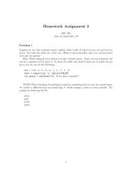
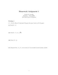
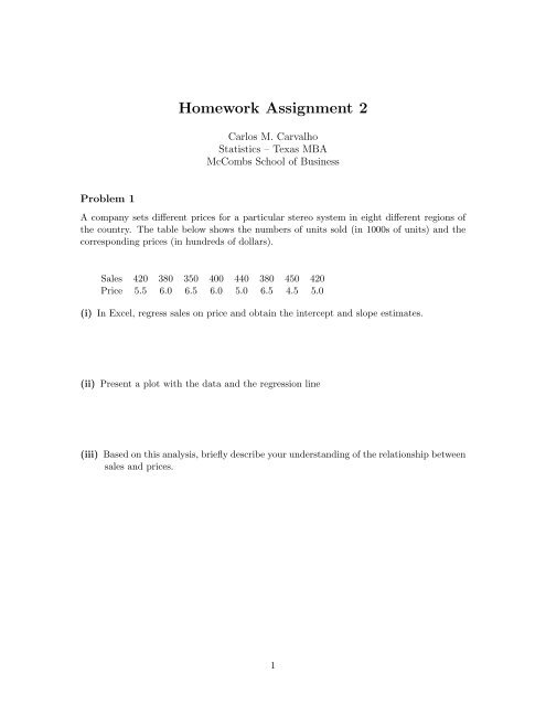
Problem 1<br />
A company sets different prices for a particular stereo system in eight different regions <strong>of</strong><br />
the country. The table below shows the numbers <strong>of</strong> units sold (in 1000s <strong>of</strong> units) and the<br />
corresponding prices (in hundreds <strong>of</strong> dollars).<br />
Sales 420 380 350 400 440 380 450 420<br />
Price 5.5 6.0 6.5 6.0 5.0 6.5 4.5 5.0<br />
(i) In Excel, regress sales on price and obtain the intercept and slope estimates.<br />
(ii) Present a plot with the data and the regression line<br />
(iii) Based on this analysis, briefly describe your understanding <strong>of</strong> the relationship between<br />
sales and prices.<br />
1
Problem 2: Match the Plots<br />
Below (Figure 1) are 4 different scatter plots <strong>of</strong> an outcome variable y versus predictor x<br />
followed by 4 four regression output summaries labeled A, B, C and D. Match the outputs<br />
with the plots.<br />
Figure 1: Scatter Plots<br />
2
Regression A:<br />
Coefficients:<br />
Estimate Std. Error<br />
(Intercept) 7.03747 0.12302<br />
(Slope) 2.18658 0.07801<br />
---<br />
Residual standard error: 1.226<br />
R-Squared: 0.8891<br />
Regression B:<br />
Coefficients:<br />
Estimate Std. Error<br />
(Intercept) 1.1491 0.1013<br />
(Slope) 1.4896 0.0583<br />
Residual standard error: 1.012<br />
R-Squared: 0.8695<br />
Regression C:<br />
Coefficients:<br />
Estimate Std. Error<br />
(Intercept) 1.2486 0.2053<br />
(Slope) 1.5659 0.1119<br />
Residual standard error: 2.052<br />
R-Squared: 0.6666<br />
Regression D:<br />
Coefficients:<br />
Estimate Std. Error<br />
(Intercept) 9.0225 0.0904<br />
(Slope) 2.0718 0.0270<br />
---<br />
Residual standard error: 0.902<br />
R-Squared: 0.9835<br />
3
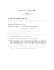
Problem 3<br />
Suppose we are modeling house price as depending on house size. Price is measured in<br />
thousands <strong>of</strong> dollars and size is measured in thousands <strong>of</strong> square feet.<br />
Suppose our model is:<br />
P = 20 + 50 s + ɛ, ɛ ∼ N(0, 15 2 ).<br />
(a) Given you know that a house has size s = 1.6, give a 95% predictive interval for the<br />
price <strong>of</strong> the house.<br />
(b) Given you know that a house has size s = 2.2, give a 95% predictive interval for the<br />
price.<br />
(c) In our model the slope is 50. What are the units <strong>of</strong> this number?<br />
(d) What are the units <strong>of</strong> the intercept 20?<br />
(e) What are the units <strong>of</strong> the the error standard deviation 15?<br />
(f) Suppose we change the units <strong>of</strong> price to dollars and size to square feet<br />
What would the values and units <strong>of</strong> the intercept, slope, and error standard deviation?<br />
(g) If we plug s = 1.6 into our model equation, P is a constant plus the normal random<br />
variables ɛ. Given s = 1.6, what is the distribution <strong>of</strong> P ?<br />
4
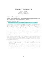
Problem 4: The Shock Absorber Data<br />
The data comes from a company which supplies a major automobile manufacturer with<br />
shock absorbers. An important characteristic is the “force transferred through the shock<br />
absorber when the shank is forced out <strong>of</strong> the cylinder”. If you don’t know what that really<br />
means, don’t worry, neither do I.<br />
What we do need to understand is that the manufacturer only considers the shock to be an<br />
acceptable part if the force measurement is between 485 and 585.<br />
The shock manufacturer and the auto manufacturer are arguing over the following issue.<br />
Before the shock is finally shipped, it is filled with gas. After it is filled with gas, it<br />
becomes very difficult to measure the force characteristic we are interested in. The shock<br />
manufacturers would like to make the measurement before the shock is filled with gas. The<br />
auto maker is concerned that there may be a difference in the force before and after the<br />
shock is filled with gas and so would like to make the measurement after it is filled.<br />
The shock maker claims that there is little difference between the before and after measurement<br />
so that the before measurement can be used.<br />
To investigate this we have the before (column 1, reboundb) and the after (column 2,<br />
rebounda) measurements on 35 shocks. The data for this problem is in shock.xls available<br />
in the class website.<br />
(a) Plot the before measurement vs. the after measurement. Does this look like the kind<br />
<strong>of</strong> data we can use the simple linear regression model to think about? Why does it<br />
make sense to choose the after measurement as “Y” and the before measurement as<br />
“X”?<br />
(b) What are 95% confidence intervals for both the slope and the intercept?<br />
(c) Test the null hypothesis H o : β 0 = 0.<br />
(d) From the shock maker’s point <strong>of</strong> view, what hypotheses would be <strong>of</strong> interest to test for<br />
the slope and intercept. That is, what would the shock maker like the true intercept<br />
and slope to be?<br />
Test whether the intercept is equal to the value proposed by the shock maker.<br />
Test whether the slope is equal to the value proposed by the shock maker.<br />
(f) Suppose the before measurement is 550.<br />
What is the plug-in predictive interval given x-before=550.<br />
What does this interval suggest about the acceptability <strong>of</strong> the shock absorber?<br />
5
Problem 5<br />
Read the case “Waite First Securities” in the course packet. The data file is available in<br />
the course website. Consider the regression model<br />
T I t = α + βSP 500 t + ɛ t ɛ t ∼ N(0, σ 2 )<br />
where T I t represents the return on Texas Instruments in month t and SP 500 t represents<br />
the return on the S&P 500 in month t.<br />
(a) What is the interpretation <strong>of</strong> β in terms <strong>of</strong> a measure <strong>of</strong> risk <strong>of</strong> the stock?<br />
(b) Plot T I against SP 500. What graphical evidence is there <strong>of</strong> a relationship between<br />
T I and SP 500? Does the relationship appear to be linear? Why or why not?<br />
(c) Estimate β. What is the interpretation <strong>of</strong> this estimate in terms <strong>of</strong> the risk <strong>of</strong> the<br />
stock? Why is Mr. Gagnon interested in this estimate?<br />
(d) Is the estimate <strong>of</strong> β obtained in part (c) the actual value <strong>of</strong> β? Why or why not?<br />
(e) Now consider the regression models<br />
Hilton t = α + βSP 500 t + ɛ t ɛ t ∼ N(0, σ 2 )<br />
where Hilton t represents the return on Hilton in month t, and<br />
Giant t = α + βSP 500 t + ɛ t ɛ t ∼ N(0, σ 2 )<br />
where Giant t represents the return on Giant in month t. How does the beta risk <strong>of</strong><br />
the three companies compare? If Mr. Gagnon wants to lower the overall market risk<br />
<strong>of</strong> his portfolio should he buy Giant, Hilton or Texas Instruments?<br />
6
Problem 6<br />
Read the “Milk and Money” case in the course notebook. The data file is available in the<br />
class website.<br />
Important information:<br />
1. The Federal government, through the Agricultural Marketing Service (AMS), sets the<br />
price that dairy farmers receive for different “classes” <strong>of</strong> milk (these classes are called<br />
Class I, Class II, etc.). The prices set by the AMS depend on, among other things,<br />
the wholesale price <strong>of</strong> milk and can vary significantly over a two or three year period.<br />
In this problem, we will be concerned only with Class III milk prices.<br />
2. A farmer can purchase a put option that gives him the right but not the obligation to<br />
sell a futures contract on Class III milk at the “strike” price on or before the expiration<br />
date <strong>of</strong> the option. This puts a “floor” under the price that the farmer will receive for<br />
his Class III milk. He removes the downside risk but still has the upside potential.<br />
For example, suppose the strike price on a December 15 Class III milk put option is<br />
$12/cwt (cwt is a unit <strong>of</strong> measurement that is roughly 100 pounds <strong>of</strong> milk). If the<br />
AMS price on December 15 is below $12/cwt, the put option allows the farmer to sell<br />
his milk for $12/cwt. If the AMS price is greater than $12/cwt then he will sell his<br />
milk at the AMS price.<br />
The cost <strong>of</strong> the put option is the price a farmer must pay someone to take on the<br />
downside risk. For example, the cost <strong>of</strong> a $12/cwt December 15 put option purchased<br />
in June might be $0.45/cwt.<br />
The farmer must also pay trading costs for purchasing the option (e.g. brokers commission,<br />
etc.). For example, the trading cost on a $12/cwt December 15 option might<br />
be $0.05/cwt.<br />
Strike prices on put options for Class III milk are available every $0.25. For example,<br />
$11.50/cwt, $11.75/cwt, $12/cwt, $12.25/cwt, etc.<br />
3. For historical and legal reasons, California dairy farmers participate in a California<br />
pricing system rather than the federal AMS pricing system. The price a California<br />
dairy farmer receives for his milk, called the “mailbox” price, is determined by a<br />
complex formula that depends on the value <strong>of</strong> various dairy products on the wholesale<br />
market. The California mailbox price varies a great deal over time just as the federal<br />
AMS price does. For example, between 2005 and 2007 the mailbox price varied<br />
between $10.16/cwt and $19.98/cwt with an average price in 2006 <strong>of</strong> $11.28/cwt.<br />
The dairy farmer in the case, Gerard, estimates his costs are $12/cwt so a price <strong>of</strong><br />
$11.28/cwt creates a significant financial problem for him.<br />
4. Gerard is interested in hedging his revenue six months in advance and guaranteeing<br />
a price <strong>of</strong> at least $12/cwt for his milk. For example, in June he wants to hedge his<br />
December 15 revenue.<br />
5. Put options on the California mailbox price are not available. The federal Class III<br />
milk price is closely related, although not the same as, the California mailbox price<br />
7
that Gerard will receive. For this reason, Gerard will use put options on the federal<br />
Class III milk price to hedge his revenue.<br />
6. Gerard wants the probability to be at least 95% that his revenue will be $12/cwt or<br />
more no matter what the California mailbox price is.<br />
Parts (a) and (b) below provide an example <strong>of</strong> how to determine the value <strong>of</strong> a put option on<br />
Class III milk on its expiration date. The same idea is used in a slightly more complicated<br />
context in parts (c) – (j).<br />
The discussion <strong>of</strong> put options on pages 6-8 <strong>of</strong> the case, and in particular the example at the<br />
bottom <strong>of</strong> page 7 and top <strong>of</strong> page 8 will be helpful in answering parts (a) and (b).<br />
(a) Suppose Gerard buys a December 15 put option on Class III milk in June with a<br />
strike price <strong>of</strong> $12/cwt. If the Class III milk price on December 15 is $11.50/cwt, how<br />
much is the put option worth when it expires on this day?<br />
(b) Suppose the price for the put option in part (a) is $0.30/cwt and that the trading<br />
costs for purchasing the option are $0.05/cwt. Combining the value <strong>of</strong> the option<br />
obtained in part (a) with the cost information, what is Gerards net gain on the option<br />
(i.e. what is the value <strong>of</strong> the put option minus the option cost and trading cost)?<br />
For parts (c)–(j), suppose Gerard in June decides to hedge his December 15 revenue by<br />
purchasing a put option on Class III milk with a strike price <strong>of</strong> $14.25/cwt and an expiration<br />
date <strong>of</strong> December 15.<br />
You should do the calculations for parts (c)–(h) assuming the costs <strong>of</strong> the option are zero.<br />
A way to incorporate the additional costs into the hedging process is discussed in parts (i)<br />
and (j).<br />
(c) Plot the Class III milk price against the California mailbox price and add the estimated<br />
regression line to the plot. To add the estimated regression line right click on any data<br />
point, click on Add Trendline, click on the box above Linear, click on the Options tab,<br />
check the box next to Display equation on chart and click OK. What is the equation<br />
<strong>of</strong> the estimated regression line? How much do you expect the Class III milk price to<br />
change on average for a $1/cwt change in the California mailbox price?<br />
For the remainder <strong>of</strong> the problem use 0.60 as the value <strong>of</strong> σ (the standard deviation <strong>of</strong> the<br />
error term) and the estimated regression line as if it were the true regression line to answer<br />
the following questions.<br />
(d) What is the probability that Gerards December 15 put option on Class III milk with<br />
a strike price <strong>of</strong> $14.25 is in the money (i.e. worth something) on December 15 if the<br />
California mailbox price on December 15 is $12.50/cwt?<br />
(e) Suppose the California mailbox price on December 15 is $12.00/cwt. What is the<br />
probability that the value <strong>of</strong> the put option will be greater than $0.50?<br />
8
(f) Using your answer to part (e), what is the probability that Gerards net revenue<br />
(mailbox price plus pay<strong>of</strong>f from the option) will exceed $12.50/cwt if the California<br />
mailbox price is $12.00/cwt?<br />
(g) Now suppose the mailbox price on December 15 is $11.50/cwt. What is the probability<br />
that the value <strong>of</strong> the put option will be greater than $1? Using your answer to this<br />
question, what is the probability that Gerards net revenue (mailbox price plus pay<strong>of</strong>f<br />
from the option) will exceed $12.50/cwt?<br />
(h) Is the probability at least 95% that his net revenue (mailbox price plus pay<strong>of</strong>f from<br />
the option) will equal or exceed $12.50/cwt for any mailbox price below $12.50/cwt?<br />
Why or why not?<br />
For parts (i) and (j), suppose the price in June for a December 15 put option on Class III<br />
milk with a strike price <strong>of</strong> $14.25/cwt is $0.45/cwt and the trading cost is $0.05/cwt.<br />
(i) Is the probability at least 95% that Gerards net revenue (mailbox price plus pay<strong>of</strong>f<br />
from the option minus option cost and trading cost) will equal or exceed his production<br />
costs <strong>of</strong> $12.00/cwt no matter what the California mailbox price is?<br />
(j) Has Gerard effectively hedged his net revenue (mailbox price plus pay<strong>of</strong>f from the<br />
option minus option cost and trading cost) if $12/cwt is the amount he needs to<br />
receive for his milk to cover his production costs?<br />
9
Problem 7: Presidential Election<br />
(Imagine this is October 2012!)<br />
This question is based on an analysis presented in the New York Times blog<br />
FiveThirtyEight by Nate Silver...<br />
According to the blog post, the most accurate economic indicator to predict the results <strong>of</strong> the<br />
election for an incumbent president is the election year “equivalent non-farm payroll growth”<br />
(in number <strong>of</strong> jobs from Jan to Oct). In the blog they provided a picture summarizing the<br />
relationship between this economic indicator and the election results. The analysis was<br />
based on the last 16 elections where a sitting president was seeking re-election. The picture<br />
is displayed below:<br />
This week, The Department <strong>of</strong> Labor released the most recent employment numbers which<br />
says that the economy has added, on average, 100,000 non-farm jobs since January 2012.<br />
10
Now, I am a gambling person and I need your help... Currently, on intrade.com, I can buy<br />
or sell a future contract on Obama’s re-election for $64.7. This contract pays $100 if Obama<br />
wins (see below).<br />
1. Based on the model presented in the New York Times blog and the numbers released by<br />
the Department <strong>of</strong> Labor how should I bet on the Intrade website (i.e., should I buy or sell<br />
the future contract)? Why?<br />
2. Do you think the answer in the question above is a good idea? Why or why not?<br />
11