Geometric modeling and computer graphics of kinematic ruled ...
Geometric modeling and computer graphics of kinematic ruled ...
Geometric modeling and computer graphics of kinematic ruled ...

Create successful ePaper yourself
Turn your PDF publications into a flip-book with our unique Google optimized e-Paper software.
in this case task <strong>of</strong> constructing <strong>kinematic</strong> <strong>ruled</strong><br />
surfaces move to feasible solution on the base <strong>of</strong><br />
complex moving one axoid along another. Complex<br />
moving can be represented as a combination <strong>of</strong><br />
concerted movement such as rolling one axoid along<br />
another <strong>and</strong> translational movement <strong>of</strong> the moving<br />
axoid along the common generating line <strong>of</strong> both<br />
axoids The similar case <strong>of</strong> geometrical <strong>modeling</strong> <strong>of</strong><br />
complex moving one axoid along another on the<br />
example <strong>of</strong> moving a cone along a torse was<br />
described earlier [2, 3]. In that case complex moving<br />
was represented as a superposition <strong>of</strong> three<br />
interrelated elementary movements: rotational<br />
movement <strong>of</strong> the cone around its axis; turn <strong>of</strong> the<br />
cone axis; translational movement <strong>of</strong> the cone vertex<br />
along the torse edge-<strong>of</strong>-regression. Similar task <strong>of</strong><br />
constructing geometrical model <strong>of</strong> complex moving<br />
one-sheet hyperboloid <strong>of</strong> revolution along another<br />
one as the base for generating new <strong>kinematic</strong> <strong>ruled</strong><br />
surfaces was solved in this research.<br />
2. PRINCIPAL GEOMETRICAL<br />
MODEL OF COMPLEX MOVING<br />
One-sheet hyperboloid surface <strong>of</strong> revolution is a<br />
<strong>ruled</strong> surface, which can be constructed by the<br />
straight line rotation about the axis, if the straight<br />
line is crossed with the axis <strong>of</strong> rotation. A case <strong>of</strong><br />
two interacting axoids contacted along mutual ruling<br />
when the axoids’ axis are crossed (Fig. 1, 3, 5), has<br />
been considered in this research. In this case,<br />
complex moving one axoid along another can be<br />
represented as a superposition <strong>of</strong> three interrelated<br />
elementary movements: rotational movement <strong>of</strong> the<br />
moving axoid around its axis OZ in the moving<br />
coordinate system OXYZ connected with the moving<br />
axoid, rotational movement <strong>of</strong> the moving axoid axis<br />
OZ around the fixed axoid axis oz in the fixed<br />
coordinate system oxyz connected with the fixed<br />
axoid, <strong>and</strong> translational movement <strong>of</strong> the moving<br />
axoid along the common generating line <strong>of</strong> both<br />
axoids. The origin <strong>of</strong> the fixed coordinate system<br />
oxyz is located in the center <strong>of</strong> the waist circle <strong>of</strong> the<br />
fixed axoid. The origin <strong>of</strong> the moving coordinate<br />
system OXYZ is located in the center <strong>of</strong> the waist<br />
circle <strong>of</strong> the moving axoid.<br />
3. GEOMETRICAL MODEL №1<br />
(ONE AXOID LOCATE ON THE<br />
OUTSIDE OF ANOTHER AXOID)<br />
<strong>Geometric</strong>al model №1 is related to the case if the<br />
outside surface <strong>of</strong> the fixed axoid is revolved<br />
slipping-free by the outside surface <strong>of</strong> the<br />
corresponding moving axoid (Fig. 1). Model №1A is<br />
related to the case if moving axoid is the same as<br />
fixed axoid. Model №1B is related to the case <strong>of</strong> two<br />
contacted different axoids.<br />
3.1 <strong>Geometric</strong>al Model №1A<br />
<strong>Geometric</strong>al model №1A is related to the case if<br />
moving axoid (2) is the same as fixed axoid (1), i.e.<br />
a 1<br />
= a 2<br />
= a , c 1<br />
= c 2<br />
= c , where<br />
a1<br />
, c1<br />
– parameters <strong>of</strong> the fixed axoid,<br />
, c – parameters <strong>of</strong> the moving axoid.<br />
a2<br />
2<br />
Parameters a, c – parameters <strong>of</strong> the canonical<br />
equation <strong>of</strong> one-sheet hyperboloid surface <strong>of</strong><br />
revolution in the coordinate system oxyz:<br />
2 2 2<br />
x y z<br />
+ − = 1 , where a – radius <strong>of</strong> waist circle.<br />
2 2 2<br />
a a c<br />
Parametric equations <strong>of</strong> surface generated by one <strong>of</strong><br />
the ruling <strong>of</strong> the moving axoid in the system OXYZ:<br />
X = R( v cos( ϕ + α)<br />
− ( v −1)cos(<br />
ϕ −α))<br />
;<br />
Y = R( vsin(<br />
ϕ + α)<br />
− ( v −1)sin(<br />
ϕ −α))<br />
;<br />
Z = −h( 2v<br />
−1)<br />
,<br />
where R – radius <strong>of</strong> circular section <strong>of</strong> one-sheet<br />
hyperboloid <strong>of</strong> revolution at h distance from the<br />
2<br />
waist section: R = a 1+<br />
( h / c)<br />
; α = arctg ( h / с)<br />
;<br />
ϕ – current value <strong>of</strong> the angle <strong>of</strong> rotation <strong>of</strong> the<br />
moving axoid around its axis, v – input parameter.<br />
The equations <strong>of</strong> transition from the coordinate<br />
system OXYZ to the coordinate system oxyz:<br />
x = X cosϕ<br />
− ( Y cosθ<br />
− Z sinθ<br />
)sinϕ<br />
+ 2a<br />
cosϕ<br />
y = X sinϕ<br />
+ ( Y cosθ<br />
− Z sinθ<br />
) cosϕ<br />
+ 2a<br />
sinϕ<br />
z = Y sinθ + Z cosθ ,<br />
where θ = 2arctg(<br />
a / c)<br />
.<br />
The resulting parametric equations <strong>of</strong> the <strong>kinematic</strong><br />
<strong>ruled</strong> surface in the fixed coordinate system oxyz:<br />
x = ( A + 2a) cosϕ<br />
− ( B cosθ<br />
+ C sinθ<br />
)sin ϕ;<br />
y = ( A + 2a)sin<br />
ϕ + ( B cosθ<br />
+ C sinθ<br />
) cosϕ;<br />
z = B sinθ − C cosθ ,<br />
where<br />
A = R( v cos( ϕ + α ) − ( v −1)cos(<br />
ϕ −α))<br />
;<br />
B = R( v sin( ϕ + α ) − ( v −1)sin(<br />
ϕ − α )) ;<br />
C = h( 2v<br />
−1)<br />
.<br />
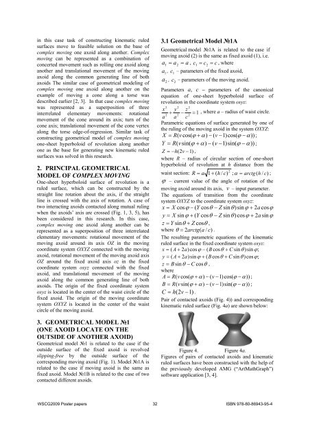
Pair <strong>of</strong> contacted axoids (Fig. 4)) <strong>and</strong> corresponding<br />
<strong>kinematic</strong> <strong>ruled</strong> surface (Fig. 4a) are shown below:<br />
Figure 4. Figure 4a.<br />
Figures <strong>of</strong> pairs <strong>of</strong> contacted axoids <strong>and</strong> <strong>kinematic</strong><br />
<strong>ruled</strong> surfaces have been constructed with the help <strong>of</strong><br />
the previously developed AMG (“ArtMathGraph”)<br />
s<strong>of</strong>tware application [3, 4].<br />
WSCG2009 Poster papers 32 ISBN 978-80-86943-95-4