assessment of the turbulence models for modelling of bubble column
assessment of the turbulence models for modelling of bubble column
assessment of the turbulence models for modelling of bubble column

You also want an ePaper? Increase the reach of your titles
YUMPU automatically turns print PDFs into web optimized ePapers that Google loves.
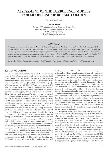
Assessment <strong>of</strong> <strong>the</strong> <strong>turbulence</strong> <strong>models</strong><br />
<strong>for</strong> <strong>modelling</strong> <strong>of</strong> <strong>bubble</strong> <strong>column</strong><br />
(Date received: 1.7.2009)<br />
Jolius Gimbun<br />
Faculty <strong>of</strong> Chemical and Natural Resources Engineering,<br />
Universiti Malaysia Pahang, Lebuhraya Tun Razak,<br />
26300 Gambang, Pahang<br />
E-mail: j.gimbun@gmail.com<br />
abstract<br />
This paper presents an Eulerian two-fluid <strong>modelling</strong> <strong>of</strong> <strong>the</strong> gas-liquid flow in a <strong>bubble</strong> <strong>column</strong>. The influence <strong>of</strong> <strong>the</strong> <strong>bubble</strong><br />
size, <strong>turbulence</strong> <strong>models</strong> and <strong>the</strong> grid size on <strong>the</strong> gas hold-up and <strong>the</strong> axial liquid velocity were evaluated. The results <strong>for</strong> <strong>the</strong><br />
gas hold-up and liquid axial velocity shows good agreement with experimental data from literature. The <strong>modelling</strong> results<br />
suggest that <strong>the</strong> two-phase k-ε <strong>turbulence</strong> model is more appropriate <strong>for</strong> <strong>bubble</strong> <strong>column</strong> operating at high gas loading (<strong>of</strong><br />
approx. 30% hold-up) and <strong>the</strong> assumption <strong>of</strong> a monodispersed <strong>bubble</strong> size is adequate <strong>for</strong> <strong>bubble</strong> <strong>column</strong> simulation.<br />
Keywords: Bubble Column, Computational Fluid Dynamics, Gas-liquid, Multiphase Modelling, and Turbulence Model<br />
1.0 INTRODUCTION<br />
A <strong>bubble</strong> <strong>column</strong> is a simple unit in which a continuous gas<br />
phase in <strong>for</strong>m <strong>of</strong> <strong>bubble</strong> moves relative to <strong>the</strong> continuous liquid<br />
phase. Bubble <strong>column</strong>s usually used as reactors in variety <strong>of</strong><br />
chemical and biochemical processes, such as oxidation reactions<br />
(e.g. [1-2]), cell cultures (e.g. [3]), alkylation reactions (e.g. [4]),<br />
effluent treatment (e.g. [5]), Fischer-Tropsch syn<strong>the</strong>sis (e.g. [6])<br />
and coal liquefaction (e.g. [7]). Bubble <strong>column</strong>s had an advantage<br />
<strong>of</strong> being mechanically simple without present <strong>of</strong> any internal<br />
structure or moving part, thus leading to easier maintenance.<br />
They also have high mass transfer rates between <strong>the</strong> gas and<br />
liquid phases, good heat transfer characteristics and large liquid<br />
hold-up, which are favourable to slow liquid phase reactions<br />
[8]. Operation <strong>of</strong> <strong>bubble</strong> <strong>column</strong>s is <strong>of</strong>ten determined by several<br />
global parameters such as pressure drop, aeration height and<br />
gas superficial velocity. However, <strong>the</strong> variables that affect <strong>the</strong><br />
per<strong>for</strong>mance <strong>of</strong> <strong>bubble</strong> <strong>column</strong> are <strong>the</strong> gas hold-up distribution,<br />
gas-liquid mass and heat transfer coefficients, <strong>the</strong> extent <strong>of</strong><br />
mixing, <strong>bubble</strong> rise velocities and <strong>bubble</strong> size distributions. It<br />
is possible to measure <strong>the</strong>se variables experimentally using, <strong>for</strong><br />
example, a combination <strong>of</strong> several instruments such as <strong>the</strong> laser<br />
doppler anemometry, dissolved oxygen probe, X-ray tomography<br />
and digital imaging. However, experimental measurements<br />
require investing in costly instruments and building a prototype.<br />
Alternatively, <strong>the</strong>se parameters can also be obtained from CFD<br />
simulations, which <strong>of</strong>fer a cheaper but much faster solution.<br />
There are many published works related to <strong>bubble</strong> <strong>column</strong><br />
<strong>modelling</strong> ranging from a simple 1D [9] to a 3D model [10-11]<br />
and some even incorporated <strong>the</strong> <strong>bubble</strong> size distributions i.e.<br />
population balance model [12-14]. Usually <strong>the</strong> Eulerian tw<strong>of</strong>luid<br />
model is employed to solve <strong>the</strong> two-phase problem and<br />
<strong>the</strong> dispersed k-ε model is used <strong>for</strong> <strong>turbulence</strong> <strong>modelling</strong>. More<br />
elaborated <strong>turbulence</strong> model such as <strong>the</strong> large eddy simulation<br />
(LES) had also been employed recently to model <strong>the</strong> two-phase<br />
flow in <strong>the</strong> <strong>bubble</strong> <strong>column</strong> [10,15]. According to Dhotre et al.<br />
[15], predictions <strong>of</strong> <strong>the</strong> mean flow field (mean velocities, mean<br />
gas hold-up) and turbulent kinetic energy obtained using <strong>the</strong> k-ε<br />
<strong>models</strong> are comparable to those obtained using LES <strong>for</strong> <strong>the</strong> case<br />
<strong>of</strong> a <strong>bubble</strong> <strong>column</strong>. This is due to <strong>the</strong> fact that <strong>the</strong>re are little<br />
chances <strong>of</strong> a high gradient flow (due to jet) or a wake flow (due<br />
to internal structure or impeller rotation) to develop in a <strong>bubble</strong><br />
<strong>column</strong> due to its simple structure. Of course <strong>the</strong> LES is a better<br />
<strong>turbulence</strong> model than <strong>the</strong> k-ε model <strong>for</strong> predicting <strong>the</strong> turbulent<br />
flow feature such as <strong>the</strong> velocity fluctuations. However, LES<br />
requires much higher computational ef<strong>for</strong>t due to needs <strong>of</strong> finer<br />
grid to better resolve <strong>the</strong> eddy structure. Since <strong>the</strong> k-ε model is<br />
capable <strong>of</strong> predicting <strong>the</strong> mean flow field satisfactorily in <strong>the</strong><br />
<strong>bubble</strong> <strong>column</strong>, thus <strong>the</strong> k-ε model was chosen instead <strong>of</strong> LES<br />
<strong>for</strong> <strong>the</strong> purpose <strong>of</strong> this study.<br />
The previous study also <strong>of</strong>ten deals with air-water system<br />
with air superficial velocity ranging from 0.012 to 0.12 m/s.<br />
There are two types <strong>of</strong> <strong>the</strong> commonly studied <strong>bubble</strong> <strong>column</strong> i.e.<br />
rectangular and cylindrical shape. Most <strong>of</strong> <strong>the</strong> studies [9-11, 15-<br />
17] employed a constant <strong>bubble</strong> size in <strong>the</strong>ir model ei<strong>the</strong>r taken<br />
from experimental observation, or computed using published<br />
correlations. Both <strong>the</strong> lift and virtual mass <strong>for</strong>ces are <strong>of</strong>ten<br />
omitted from <strong>the</strong> simulation but <strong>the</strong> drag coefficient is applied.<br />
Interestingly, most <strong>of</strong> <strong>the</strong> CFD studies on <strong>bubble</strong> <strong>column</strong>s were<br />
able to predict correctly <strong>the</strong> gas hold-up and liquid axial velocity<br />
even without applying <strong>the</strong> <strong>bubble</strong> size distribution model. The<br />
reason is that <strong>the</strong>re is little chance <strong>of</strong> <strong>for</strong>ming a <strong>bubble</strong> breakage<br />
dominated system in a <strong>bubble</strong> <strong>column</strong> and most <strong>of</strong> <strong>the</strong> coalescence<br />
taking place near <strong>the</strong> sparger. Bubble breakage occurs due to high<br />
Journal - The Institution <strong>of</strong> Engineers, Malaysia (Vol. 70, No.4, December 2009) 57<br />
057-064•Assessment <strong>of</strong> <strong>the</strong> <strong>turbulence</strong> 4pp.indd 57<br />
1/21/2010 9:50:20 AM
Jolius Gimbun<br />
gradient <strong>of</strong> turbulent kinetic energy and dissipation rates, which<br />
is <strong>of</strong>ten induced by mechanical moving part i.e. impeller. In <strong>the</strong><br />
case <strong>of</strong> <strong>bubble</strong> <strong>column</strong>, <strong>the</strong> flow is only driven by <strong>the</strong> <strong>bubble</strong> rise<br />
motion and <strong>the</strong> resultant turbulent flow is not sufficient to imply<br />
a <strong>bubble</strong> breakage dominated system. That leaves <strong>the</strong> <strong>bubble</strong> size<br />
almost constant throughout <strong>the</strong> <strong>column</strong> thus eliminating <strong>the</strong> vital<br />
needs <strong>of</strong> <strong>the</strong> population balance model (PBM). Chen et al. [12]<br />
employed a PBM in <strong>the</strong>ir work, and <strong>the</strong>y compared <strong>the</strong> result<br />
with <strong>the</strong> one without PBM. Their <strong>modelling</strong> was carried out in a<br />
2D domain. According to Chen et al. [12], CFD simulation using<br />
a monodispersed <strong>bubble</strong> size itself can match <strong>the</strong> result from a<br />
more complicated CFD-PBM. This is due to <strong>the</strong> fact that <strong>bubble</strong><br />
size in a <strong>bubble</strong> <strong>column</strong> is virtually monodispersed and hence<br />
can be represented by <strong>the</strong> mean <strong>bubble</strong> size during <strong>the</strong> CFD<br />
simulation. Similar observation was also reported by Groen [18]<br />
who per<strong>for</strong>med detailed experimental measurement on <strong>bubble</strong><br />
size distribution in a <strong>bubble</strong> <strong>column</strong>.<br />
Despite many published work on CFD <strong>of</strong> <strong>bubble</strong> <strong>column</strong>s,<br />
selection <strong>of</strong> <strong>turbulence</strong> <strong>models</strong> is still not clearly understood.<br />
To <strong>the</strong> author’s knowledge, such a study has not yet been<br />
undertaken and that is <strong>the</strong> aim <strong>of</strong> this work. In this work, three<br />
different <strong>turbulence</strong> <strong>models</strong> namely mixture k-ε, dispersed k-ε<br />
and two-phase k-ε were employed to predict <strong>the</strong> hydrodynamics<br />
<strong>of</strong> a <strong>bubble</strong> <strong>column</strong> operating at a relatively high superficial gas<br />
velocity <strong>of</strong> 0.12 m/s, which corresponds to 30% gas hold-up.<br />
2.0 Modelling approach<br />
2.1 CFD <strong>modelling</strong> <strong>of</strong> two-phase flow<br />
The Eulerian-Eulerian approach is employed <strong>for</strong> gas-liquid<br />
<strong>bubble</strong> <strong>column</strong> simulation in this work, whereby <strong>the</strong> continuous<br />
and disperse phases are considered as interpenetrating media,<br />
identified by <strong>the</strong>ir local volume fractions. The volume fractions<br />
sum to unity and are governed by <strong>the</strong> following continuity<br />
equations:<br />
∂<br />
∂t<br />
<br />
α (1)<br />
( ρ ) + ∇ ⋅( α ρ u ) = 0<br />
l<br />
l<br />
l<br />
l<br />
l<br />
where α l<br />
is <strong>the</strong> liquid volume fraction, ρ l<br />
is <strong>the</strong> density,<br />
and u l is <strong>the</strong> velocity <strong>of</strong> <strong>the</strong> liquid phase. The mass transferred<br />
between phases is negligibly small and hence is not included in<br />
<strong>the</strong> right hand-side <strong>of</strong> eq.(1). A similar equation is solved <strong>for</strong> <strong>the</strong><br />
volume fraction <strong>of</strong> <strong>the</strong> gas phase by replacing <strong>the</strong> subscript l with<br />
g <strong>for</strong> gas. The momentum balance <strong>for</strong> <strong>the</strong> liquid phase is:<br />
<br />
where τ<br />
l is <strong>the</strong> liquid phase stress-strain tensor, F<br />
lift , l<br />
is a lift<br />
<strong>for</strong>ce, g is <strong>the</strong> acceleration due to gravity and is <strong>the</strong> virtual<br />
mass <strong>for</strong>ce. A similar equation is solved <strong>for</strong> <strong>the</strong> gas phase. F <br />
l g<br />
is <strong>the</strong> interaction <strong>for</strong>ce between phases, due to drag. Hence, F ∂<br />
<br />
ρmk<br />
+ ∇ ⋅ ρmumk<br />
l ∂t<br />
g<br />
is represented by a simple interaction term <strong>for</strong> <strong>the</strong> drag <strong>for</strong>ce,<br />
given by:<br />
∂<br />
<br />
<br />
F<br />
lg<br />
3<br />
= −<br />
<br />
C u<br />
b<br />
<br />
( u − u )<br />
(2)<br />
α<br />
gαl<br />
D g<br />
−<br />
l g l<br />
(3)<br />
4d<br />
<br />
u<br />
where C D is a drag coefficient and d b is <strong>the</strong> Sauter mean<br />
<strong>bubble</strong> diameter.<br />
The drag model employed has a significant effect on <strong>the</strong><br />
flow field <strong>of</strong> <strong>the</strong> aerated flow, as it is related directly to <strong>the</strong> <strong>bubble</strong><br />
terminal rise velocity. The drag model given as a function <strong>of</strong> <strong>the</strong><br />
<strong>bubble</strong> Reynolds number, Re b , from Schiller and Naumann [19]<br />
was employed in this work:<br />
24<br />
0.687<br />
C D = –––– (1 + 0.15Re b ) (4)<br />
Re b<br />
Lift <strong>for</strong>ces act on a <strong>bubble</strong> due to <strong>the</strong> velocity gradients in<br />
<strong>the</strong> liquid phase and are said to be more significant <strong>for</strong> larger<br />
<strong>bubble</strong>s. The lift <strong>for</strong>ce acting on a gas phase in a liquid phase can<br />
be estimated from:<br />
where C L is a lift coefficient has a value 0.5. A similar lift<br />
<strong>for</strong>ce is added to <strong>the</strong> right-hand side <strong>of</strong> <strong>the</strong> momentum equation<br />
<br />
<strong>for</strong> both phases ( F<br />
lift,<br />
g<br />
= −F<br />
).<br />
lift,<br />
l<br />
The virtual mass effect occurs when a gas phase accelerates<br />
relative to <strong>the</strong> liquid phase. The fluid surrounding <strong>the</strong> <strong>bubble</strong> is<br />
accelerating as a consequence <strong>of</strong> <strong>the</strong> <strong>bubble</strong> acceleration. This<br />
gives a rise to a <strong>for</strong>ce called a virtual mass which accounts <strong>for</strong><br />
<strong>the</strong> losses <strong>of</strong> momentum <strong>of</strong> <strong>the</strong> accelerating <strong>bubble</strong>. The virtual<br />
mass <strong>for</strong>ce acting on <strong>bubble</strong>s is given by:<br />
where C m is <strong>the</strong> added mass coefficient has a value 0.5 <strong>for</strong><br />
sphere. Similar with <strong>the</strong> lift <strong>for</strong>ce <strong>the</strong> virtual mass <strong>for</strong>ce is added<br />
to <strong>the</strong> right-hand side <strong>of</strong> <strong>the</strong> momentum equation <strong>for</strong> both phases<br />
.<br />
2.2 Turbulence <strong>modelling</strong><br />
There are three different options available <strong>for</strong> <strong>turbulence</strong><br />
<strong>modelling</strong> <strong>of</strong> multiphase flow in FLUENT namely <strong>the</strong> mixture<br />
k-ε, dispersed k-ε and two-phase k-ε <strong>models</strong> [20]. All three<br />
<strong>turbulence</strong> <strong>models</strong> used <strong>the</strong> same model constants but has<br />
different equations to account <strong>for</strong> <strong>the</strong> <strong>turbulence</strong> viscosity.<br />
Mixture k-ε model<br />
The mixture <strong>turbulence</strong> model is <strong>the</strong> default multiphase<br />
<strong>turbulence</strong> model in FLUENT 6.3. It represents <strong>the</strong> first extension<br />
<strong>of</strong> <strong>the</strong> single-phase k-ε model, and it is applicable when phases<br />
separate, <strong>for</strong> stratified (or nearly stratified) multiphase flows, and<br />
when <strong>the</strong> density ratio between phases is close to 1. In <strong>the</strong>se cases,<br />
using mixture properties and mixture velocities is sufficient to<br />
capture important features <strong>of</strong> <strong>the</strong> turbulent flow.<br />
The k and ε equations describing this model are as follows:<br />
∂t<br />
⎛ µ<br />
⎜<br />
⎝ σ<br />
t,<br />
m<br />
( ) ( ) = ∇ ⋅⎜<br />
∇k<br />
⎟ G − ρ ε<br />
m<br />
µ<br />
⎜<br />
⎝ σ<br />
k<br />
⎞<br />
⎟ +<br />
⎠<br />
k , m<br />
⎛ t,<br />
m ⎞ ε<br />
( ρ ε ) + ∇ ⋅( ρ u ε ) = ∇ ⋅⎜<br />
∇ε<br />
⎟ ( C G − C ρ ε)<br />
m<br />
m<br />
m<br />
ε<br />
⎟ +<br />
⎠ k<br />
1, ε<br />
m<br />
k , m<br />
where <strong>the</strong> G k,m is <strong>the</strong> mixture turbulent kinetic production<br />
term. The mixture density and velocity, ρ m<br />
and u , are computed<br />
m<br />
from;<br />
2, ε<br />
m<br />
(5)<br />
(6)<br />
(7)<br />
(8)<br />
58<br />
Journal - The Institution <strong>of</strong> Engineers, Malaysia (Vol. 70, No.4, December 2009)<br />
057-064•Assessment <strong>of</strong> <strong>the</strong> <strong>turbulence</strong> 4pp.indd 58<br />
1/21/2010 9:50:20 AM
Assessment <strong>of</strong> <strong>the</strong> <strong>turbulence</strong> <strong>models</strong> <strong>for</strong> <strong>modelling</strong> <strong>of</strong> <strong>bubble</strong> <strong>column</strong><br />
N<br />
∑<br />
ρ<br />
m<br />
= αiρi<br />
(9)<br />
i=<br />
1<br />
and<br />
N<br />
N<br />
u m<br />
= α ρ u<br />
α ρ<br />
(10)<br />
∑<br />
i=<br />
1<br />
i<br />
i<br />
i<br />
∑<br />
i=<br />
1<br />
i<br />
i<br />
The turbulent viscosity, µ tm , is computed from<br />
2<br />
k<br />
t , m<br />
= ρmC<br />
(11)<br />
ε<br />
µ<br />
µ<br />
The model constants are; C ε1<br />
= 1.44, C ε2<br />
= 1.2, C ε3<br />
= 1.2,<br />
C µ<br />
= 0.09, σ k<br />
= 1 and σ ε<br />
= 1.3.<br />
Dispersed k-ε model<br />
Dispersed k-ε model is suitable when <strong>the</strong> secondary phase is<br />
dilute and <strong>the</strong> primary phase is clearly continuous, <strong>the</strong> dispersed<br />
k-ε <strong>turbulence</strong> model is used and solves <strong>the</strong> standard k-ε<br />
equations <strong>for</strong> <strong>the</strong> primary phase. The liquid turbulent viscosity,<br />
μ t,l<br />
, is written as:<br />
k<br />
,<br />
= (12)<br />
2<br />
l<br />
µ<br />
t l<br />
ρlCµ<br />
ε<br />
l<br />
The transport equations <strong>for</strong> k and ε in <strong>the</strong> dispersed k-ε<br />
model are given by:<br />
(13)<br />
(14)<br />
G k,l<br />
is <strong>the</strong> rate <strong>of</strong> production <strong>of</strong> turbulent kinetic energy and<br />
it has a similar <strong>for</strong>m to <strong>the</strong> one applied <strong>for</strong> single phase flow. The<br />
terms ∏ k,l<br />
and ∏ ε,l<br />
represent <strong>the</strong> influence <strong>of</strong> <strong>the</strong> dispersed phase<br />
on <strong>the</strong> continuous phase and are modelled following Elgobashi<br />
and Abou-Arab [21]. The turbulent quantities <strong>for</strong> <strong>the</strong> dispersed<br />
phase like turbulent kinetic energy and turbulent viscosity <strong>of</strong> <strong>the</strong><br />
gas are modelled following Mudde and Simonin [22] using <strong>the</strong><br />
primary phase turbulent quantities [20]. The model constants are<br />
similar to those <strong>of</strong> mixture k-ε <strong>models</strong>.<br />
Two-phase k-ε model<br />
The most general <strong>turbulence</strong> model <strong>for</strong> multiphase flows<br />
solves a set <strong>of</strong> k and ε transport equations <strong>for</strong> each phase. This<br />
<strong>turbulence</strong> model is <strong>the</strong> appropriate choice when <strong>the</strong> <strong>turbulence</strong><br />
transfer among <strong>the</strong> phases plays a dominant role i.e. high gas<br />
void fraction. The transport equations <strong>for</strong> two-phase k-ε model<br />
are given by:<br />
∂<br />
∂t<br />
N<br />
∑<br />
l = 1<br />
<br />
⎛<br />
⎜<br />
⎝<br />
⎞<br />
⎟ +<br />
⎠<br />
t,<br />
l<br />
( α k ) + ∇ ⋅( ρ α u k ) = ∇ ⋅⎜α<br />
∇k<br />
⎟ ( α G −α<br />
ρ ε )+<br />
ρ<br />
l l l<br />
l l l l<br />
l<br />
l l k , l<br />
σ<br />
k<br />
K<br />
g l<br />
µ<br />
N<br />
N<br />
µ<br />
t,<br />
g<br />
µ<br />
l<br />
( ) ( ) ( ) t ,<br />
Cg<br />
lkg<br />
− Cl<br />
gkl<br />
− K<br />
g l<br />
ug<br />
− ul<br />
⋅ ∇α<br />
g<br />
+ K<br />
g l<br />
ug<br />
− ul<br />
⋅ ∇αl<br />
∑<br />
g = 1<br />
α σ<br />
g<br />
g<br />
∑<br />
g = 1<br />
l<br />
l<br />
l<br />
αlσ<br />
l<br />
(15)<br />
∂<br />
∂t<br />
C<br />
t,<br />
l<br />
l<br />
( ρ α ε ) + ∇ ⋅( ρ α u ε ) = ∇ ⋅⎜α<br />
∇ε<br />
⎟ C α G − C α ρ ε +<br />
⎛<br />
⎜<br />
⎝<br />
l<br />
N<br />
∑<br />
l<br />
3, ε<br />
l = 1<br />
C l g<br />
K<br />
l<br />
g l<br />
l<br />
l<br />
<br />
l<br />
l<br />
⎛ µ ⎞ ⎡<br />
⎟ + ε<br />
⎜ l<br />
l ⎢<br />
⎝ σ<br />
ε ⎠ kl<br />
⎣<br />
µ<br />
g<br />
− ⋅<br />
t ,<br />
K<br />
g l<br />
ug<br />
ul<br />
∇α<br />
g<br />
+<br />
α σ<br />
1, ε<br />
l<br />
k , l<br />
N<br />
N<br />
<br />
( C k − C k ) − ( ) K ( u − u ) ⋅<br />
g l g<br />
l g l<br />
∑<br />
g = 1<br />
Term C gl<br />
= 2 and C lg<br />
are given as:<br />
g<br />
g<br />
∑<br />
g = 1<br />
g l<br />
g<br />
l<br />
2, ε<br />
l<br />
µ ⎞⎤<br />
t,<br />
l<br />
∇α<br />
⎟<br />
l<br />
⎥<br />
αlσ<br />
l ⎠⎥⎦<br />
l<br />
l<br />
(16)<br />
⎛ η ⎞<br />
r<br />
= 2 ⎜<br />
⎟<br />
(17)<br />
⎝1+<br />
ηr<br />
⎠<br />
The turbulent viscosity <strong>for</strong> each phase l is given as<br />
follows:<br />
k<br />
,<br />
= (18)<br />
2<br />
l<br />
µ<br />
t l<br />
ρlCµ<br />
ε<br />
l<br />
The model constants are similar to those <strong>of</strong> mixture k-ε<br />
<strong>models</strong>.<br />
2.3 Bubble <strong>column</strong> dimensions and <strong>modelling</strong> strategy<br />
A cylindrical <strong>bubble</strong> <strong>column</strong> was considered with a diameter<br />
<strong>of</strong> 0.19 m, filled with tap water to a height <strong>of</strong> 0.96 m; a per<strong>for</strong>ated<br />
plate sparger was placed at <strong>the</strong> bottom <strong>of</strong> <strong>the</strong> <strong>column</strong>. The gas<br />
superficial velocity was 0.12 m/s. The geometry <strong>of</strong> <strong>the</strong> <strong>bubble</strong><br />
<strong>column</strong> studied here was similar to <strong>the</strong> one that has been studied<br />
experimentally by Degaleesan [24] and, which has been simulated<br />
numerically by Sanyal et al. [16] and Chen et al. [12].<br />
Usually, fine <strong>bubble</strong>s introduced by sparger will coalesce<br />
immediately when <strong>the</strong>y come in contact with <strong>the</strong> neighbouring<br />
<strong>bubble</strong>s. The upward movement <strong>of</strong> <strong>the</strong> <strong>bubble</strong> induces <strong>the</strong><br />
turbulent flow due to upward and downward movement <strong>of</strong> <strong>the</strong><br />
liquid phase as <strong>the</strong> <strong>bubble</strong> rises. The turbulent flow would <strong>the</strong>n<br />
induce <strong>the</strong> <strong>bubble</strong> breakage and coalescence, which would attain<br />
equilibrium when a certain size <strong>of</strong> <strong>bubble</strong> has been obtained. It<br />
has to be noted that <strong>the</strong> gas sparging rate need to be controlled<br />
to ensure a better gas dispersion in a <strong>bubble</strong> <strong>column</strong>. At lower<br />
gas flow rate, <strong>the</strong> <strong>bubble</strong> <strong>column</strong> operates under a homogeneous<br />
bubbly flow regime, if <strong>the</strong> gas flow rate increased even fur<strong>the</strong>r<br />
<strong>the</strong> flow regime may become turbulent bubbly flow or slug and<br />
annular flow <strong>for</strong> even higher gas flow rate. The flow regime<br />
transition in <strong>the</strong> <strong>bubble</strong> <strong>column</strong> cannot be generalised by looking<br />
at its relationship with <strong>the</strong> gas flow rate alone because <strong>the</strong>y are<br />
dependent upon many o<strong>the</strong>r parameters such as <strong>the</strong> <strong>column</strong><br />
geometry, material properties and operating conditions. Fur<strong>the</strong>r<br />
details regarding <strong>the</strong> flow regime transition in a <strong>bubble</strong> <strong>column</strong><br />
may be understood better by referring to a recent review by<br />
Shaikh and Al-Dahhan [23].<br />
The Eulerian two-fluid model was employed throughout<br />
this study with constant <strong>bubble</strong> sizes <strong>of</strong> 3.6 mm, 4.4 mm and<br />
7 mm. The transient solvers with second order implicit time<br />
advancement and <strong>the</strong> third-order (QUICK) spatial interpolation<br />
schemes were also applied. The interphase drag coefficient was<br />
estimated using <strong>the</strong> Schiller-Naumann drag model and virtual<br />
mass was also included. The top liquid surface was allowed to<br />
expand freely as a result <strong>of</strong> aeration by applying a free surface<br />
boundary.<br />
Two grid sizes were evaluated in this study, which is<br />
labelled as coarse (Figure 1A) and fine (Figure 1B) generated by<br />
Journal - The Institution <strong>of</strong> Engineers, Malaysia (Vol. 70, No.4, December 2009) 59<br />
057-064•Assessment <strong>of</strong> <strong>the</strong> <strong>turbulence</strong> 4pp.indd 59<br />
1/21/2010 9:50:21 AM
Jolius Gimbun<br />
pre-processor s<strong>of</strong>tware, GAMBIT 2.2. The coarse grid contains<br />
6150 cells and <strong>the</strong> fine one contains 43460 cells. Both grids were<br />
made <strong>of</strong> a high quality pure hexahedral mesh to minimise <strong>the</strong><br />
turbulent diffusion during <strong>the</strong> simulation. Grid refinement was<br />
carried out in FLUENT after a steady aeration level was reached<br />
based on <strong>the</strong> aerated water level in <strong>the</strong> <strong>column</strong>. The grid refinement<br />
was applied in <strong>the</strong> cells where <strong>the</strong> water volume fraction is<br />
greater than 0.04. Such a method is good <strong>for</strong> grid economy,<br />
because only <strong>the</strong> section containing liquid will be refined, thus<br />
making <strong>the</strong> excess (headspace) volume just represent a mere 2%<br />
<strong>of</strong> <strong>the</strong> total cells count. The excess volume in <strong>the</strong> headspace is<br />
necessary because at <strong>the</strong> initial stages <strong>of</strong> <strong>the</strong> simulation, <strong>the</strong>re are<br />
some major fluctuations <strong>of</strong> <strong>the</strong> liquid surface; without this excess<br />
volume, some part <strong>of</strong> <strong>the</strong> liquid would flow out from <strong>the</strong> domain<br />
and hence may cause error to <strong>the</strong> final result. This incidence is<br />
shown in Figure 2 which was simulated using a grid <strong>of</strong> only 1.4<br />
m height. In <strong>the</strong> third frame, <strong>the</strong> aerated level exceeds <strong>the</strong> upper<br />
bound <strong>of</strong> <strong>the</strong> flow domain, which is unacceptable. In light with this<br />
issue, <strong>the</strong> final grid height was extended up to 1.5 m, to provide a<br />
more satisfactory simulation. The evidence <strong>of</strong> a turbulent bubbly<br />
flow is also depicted in Figure 2 as <strong>the</strong> flow becomes unstable<br />
and <strong>the</strong> <strong>bubble</strong>s cluster into swarms, hence regions <strong>of</strong> relatively<br />
high and low gas fractions can be distinguished. The motion <strong>of</strong><br />
swarms through <strong>the</strong> <strong>column</strong> is highly irregular and <strong>the</strong> swarms<br />
only exist <strong>for</strong> a short period <strong>of</strong> time [18]. The swarms dominate<br />
<strong>the</strong> hydrodynamic behavior <strong>of</strong> a <strong>bubble</strong> <strong>column</strong> by increasing <strong>the</strong><br />
degree <strong>of</strong> (back) mixing or dispersion <strong>of</strong> <strong>the</strong> liquid phase leading<br />
to larger-scale circulation patterns. The long-time-averaged<br />
liquid flow field shows a large overall liquid circulation pattern<br />
with <strong>the</strong> liquid phase flows upward in <strong>the</strong> centre <strong>of</strong> <strong>the</strong> <strong>column</strong><br />
and downward in <strong>the</strong> wall region [18].<br />
The coarse grid employed in this work may not be capable<br />
<strong>of</strong> resolving correctly <strong>the</strong> <strong>turbulence</strong> related quantities (k and ε),<br />
but it is assumed to have a limited effect in this study, since <strong>the</strong><br />
<strong>bubble</strong> size distribution model is not included; instead <strong>bubble</strong><br />
is assumed to be monodispersed in this study. The <strong>turbulence</strong><br />
related quantities must be resolved <strong>for</strong> better prediction <strong>of</strong><br />
<strong>bubble</strong> size when a <strong>bubble</strong> size distribution model is employed<br />
as <strong>the</strong> turbulent dissipation rates have a great influence on <strong>bubble</strong><br />
coalescence and break-up. All result presented in this chapter are<br />
taken at z = 0.53 and are time-averages <strong>of</strong> up to 1000 time step<br />
after a steady aerated liquid level is attained. During <strong>the</strong> initial<br />
simulation prior to achieving <strong>the</strong> pseudo-steady aerated liquid<br />
level a much larger time step <strong>of</strong> 0.01 s was employed. The time<br />
step was reduced to 0.005 s <strong>for</strong> <strong>the</strong> final simulation and were<br />
averaged <strong>for</strong> <strong>the</strong> real time <strong>of</strong> 5 seconds.<br />
Water with a volume fraction <strong>of</strong> 1.0 is patched to 0 ≤ z ≥<br />
0.96 (initial liquid height) be<strong>for</strong>e running <strong>the</strong> simulation, whereas<br />
water volume fraction <strong>of</strong> 0 is patched to <strong>the</strong> headspace (0.96 ≤<br />
z ≤ 1.5). Air is sparged at <strong>the</strong> bottom <strong>of</strong> <strong>the</strong> <strong>column</strong> using a<br />
velocity inlet boundary (gas inlet velocity equal to superficial gas<br />
velocity) as soon as <strong>the</strong> simulation started (time = 0 s).<br />
Figure 1: Surface mesh <strong>of</strong> <strong>the</strong> <strong>bubble</strong> <strong>column</strong> , A) Coarse mesh, B)<br />
Fine mesh<br />
Figure 2: Illustration <strong>of</strong> liquid overflowing from <strong>the</strong> flow domain (t = 3.49~3.58 s) in <strong>the</strong> initial stage <strong>of</strong> <strong>the</strong> simulation <strong>for</strong> <strong>the</strong> case with grid<br />
height <strong>of</strong> 1.4 m. The image is coloured by gas volume fraction and so <strong>the</strong> red upper layer represents <strong>the</strong> headspace<br />
60<br />
Journal - The Institution <strong>of</strong> Engineers, Malaysia (Vol. 70, No.4, December 2009)<br />
057-064•Assessment <strong>of</strong> <strong>the</strong> <strong>turbulence</strong> 4pp.indd 60<br />
1/21/2010 9:50:21 AM
Assessment <strong>of</strong> <strong>the</strong> <strong>turbulence</strong> <strong>models</strong> <strong>for</strong> <strong>modelling</strong> <strong>of</strong> <strong>bubble</strong> <strong>column</strong><br />
3.0 Results and Discussions<br />
3.1 Effect <strong>of</strong> <strong>the</strong> <strong>bubble</strong> size<br />
Correlations to estimate <strong>the</strong> mean <strong>bubble</strong> size are <strong>of</strong>ten<br />
related to liquid surface tension (σ), liquid density (ρ l ), liquid<br />
viscosity (μ l ) and gas superficial velocity (v sg ). Some correlations<br />
include <strong>the</strong> gas density (ρ g ) and gravity (g) as well, such as <strong>the</strong><br />
one proposed by Wilkinson [25]:<br />
d b = 3g -0.44 σ 0.34 µ l<br />
0.22<br />
ρ l<br />
-0.45<br />
ρ g<br />
-0.11<br />
v sg<br />
-0.02<br />
(19)<br />
Ano<strong>the</strong>r correlation <strong>of</strong> <strong>bubble</strong> size proposed by Pohorecki<br />
et al. [26] is:<br />
d b = 0.289 σ 0.442 µ l<br />
-0.048<br />
ρ l<br />
-0.552<br />
v sg<br />
-0.124<br />
(20)<br />
Both correlations give a mean <strong>bubble</strong> size less than 5 mm<br />
i.e. 4.4 mm <strong>for</strong> Wilkinson and 3.6 mm <strong>for</strong> Pohorecki. These<br />
values are in good agreement with Deen et al.’s [10] experiments,<br />
which observed a 4 mm mean <strong>bubble</strong> diameter in his study on a<br />
rectangular <strong>bubble</strong> <strong>column</strong> <strong>of</strong> air-water system.<br />
Comparisons <strong>of</strong> <strong>the</strong> CFD prediction <strong>for</strong> <strong>the</strong> three different<br />
<strong>bubble</strong> sizes are shown in Figures 3 and 4, alongside <strong>the</strong><br />
experimental data <strong>of</strong> Degaleesan [24]. There is no noteworthy<br />
difference between <strong>the</strong> liquid axial velocity and gas holdup<br />
calculated using <strong>the</strong> <strong>bubble</strong> size <strong>of</strong> ei<strong>the</strong>r 4.4 mm or<br />
3.6 mm (Figure 5.4), maybe because <strong>the</strong> difference <strong>of</strong> <strong>the</strong> <strong>bubble</strong><br />
size is just a mere 0.8 mm and thus <strong>the</strong> effect is insignificant.<br />
Meanwhile, both <strong>the</strong> gas hold-up and liquid axial velocity were<br />
underpredicted when <strong>the</strong> 7 mm <strong>bubble</strong> diameter was applied.<br />
This underprediction <strong>of</strong> <strong>the</strong> gas hold-up is due to <strong>the</strong> fact that<br />
bigger <strong>bubble</strong>s tend to rise faster than smaller ones and thus <strong>the</strong><br />
gas volume fraction in <strong>the</strong> liquid is reduced. The liquid velocity<br />
is affected by <strong>the</strong> <strong>bubble</strong> size: bigger <strong>bubble</strong>s might increase<br />
<strong>the</strong> axial velocity due to <strong>the</strong>ir larger <strong>bubble</strong> rise velocity but<br />
at <strong>the</strong> same time <strong>the</strong> downward recirculation also becomes<br />
larger. In fact, <strong>the</strong> momentum from <strong>the</strong> liquid recirculation<br />
is bigger than <strong>the</strong> one induced by <strong>bubble</strong> rise velocity, and<br />
<strong>the</strong>re<strong>for</strong>e a bigger <strong>bubble</strong> size leads to a lower axial liquid<br />
velocity.<br />
Figure 3: Effect <strong>of</strong> <strong>bubble</strong> size on gas hold-up and axial liquid velocity, <strong>modelling</strong> were carried out using <strong>the</strong> fine grid<br />
3.2 Assessment <strong>of</strong> <strong>the</strong> <strong>modelling</strong> grid<br />
The initial grid was quite coarse (approx 2 x 2 x 1.5 cm)<br />
and contained only 6150 computational cells as shown in Figure<br />
1A. Initial iterations were carried out on <strong>the</strong> coarse grid until<br />
a pseudo-steady aerated liquid height was reached. Then a grid<br />
adaptation was applied in <strong>the</strong> region where <strong>the</strong> water volume<br />
fraction was greater than 0.4 (up to <strong>the</strong> aerated liquid height). As<br />
a result a relatively fine grid containing 43 460 cells (see Figure<br />
1B) was created. For grid <strong>assessment</strong> purpose, <strong>the</strong> simulation<br />
was <strong>the</strong>n carried out using both grids with <strong>the</strong> mixture k-ε<br />
model <strong>for</strong> <strong>turbulence</strong> and <strong>the</strong> two phase flow was modelled via<br />
<strong>the</strong> Eulerian-Eularian model. The mixture k-ε model itself uses<br />
exactly similar equation to <strong>the</strong> standard k-ε <strong>for</strong>mulation, except<br />
that <strong>the</strong> physical and <strong>the</strong>rmodynamic properties <strong>of</strong> <strong>the</strong> mixture are<br />
applied.<br />
The effect <strong>of</strong> grid size on two-phase flow in a <strong>bubble</strong><br />
<strong>column</strong> is presented in Figure 4. It was found that <strong>the</strong> finer grid<br />
gave a slightly higher peak <strong>of</strong> <strong>the</strong> gas hold - up and liquid axial<br />
velocity, as shown in Figure 4, which is closer to Degaleesan’s<br />
experimental data. Finer grids also help to resolve correctly<br />
<strong>the</strong> gas hold-up and liquid axial velocity very close to <strong>the</strong> wall,<br />
which is not shown in a coarser grid. There<strong>for</strong>e, <strong>the</strong> finer grid<br />
will be employed <strong>for</strong> <strong>the</strong> rest <strong>of</strong> <strong>the</strong> study in this case as it gave<br />
much closer agreement with Degaleesan’s experimental data.<br />
The use <strong>of</strong> a finer grid, however, poses a significant increase in<br />
computational ef<strong>for</strong>t with nearly ten times slower iterations than<br />
<strong>the</strong> coarser one. It should be noted that effect <strong>of</strong> <strong>the</strong> grid refinement<br />
is not very obvious in this study due to several reasons. Firstly,<br />
<strong>the</strong> grid employed in this work are made <strong>of</strong> pure hexahedral<br />
aligned to <strong>the</strong> mean flow direction hence minimising <strong>the</strong> turbulent<br />
diffusion thus resulting in better prediction. Secondly, <strong>the</strong> close<br />
agreement between <strong>the</strong> result obtained from both fine and coarse<br />
grid actually confirming a grid independent solution has been<br />
achieved.<br />
Journal - The Institution <strong>of</strong> Engineers, Malaysia (Vol. 70, No.4, December 2009) 61<br />
057-064•Assessment <strong>of</strong> <strong>the</strong> <strong>turbulence</strong> 4pp.indd 61<br />
1/21/2010 9:50:21 AM
Jolius Gimbun<br />
Figure 4: Prediction <strong>of</strong> gas hold-up and axial liquid velocity by mixture <strong>turbulence</strong> model <strong>for</strong> different grid resolution<br />
3.3 Assessment <strong>of</strong> <strong>the</strong> <strong>turbulence</strong> <strong>models</strong><br />
There are three <strong>turbulence</strong> model available <strong>for</strong> multiphase<br />
<strong>modelling</strong> in FLUENT namely, mixture k-ε, dispersed k-ε and<br />
two-phase k-ε. The mixture model is said to be suitable <strong>for</strong> a<br />
system with a fluid density ratio close to 1, e.g. hexanol-water<br />
system. The dispersed model is applicable when <strong>the</strong>re is clearly<br />
one primary continuous phase and <strong>the</strong> remainder is a dilute<br />
secondary phase. The two-phase <strong>turbulence</strong> model is said to<br />
be an appropriate choice when <strong>the</strong> <strong>turbulence</strong> transfer among<br />
<strong>the</strong> phases plays a dominant role. However, it should be noted<br />
that <strong>the</strong> two-phase model is two times more computational<br />
intensive than ei<strong>the</strong>r <strong>the</strong> dispersed or <strong>the</strong> mixture <strong>models</strong>, since<br />
<strong>the</strong> <strong>turbulence</strong> model must be solved <strong>for</strong> both phases <strong>for</strong> each<br />
iteration. Since <strong>the</strong>re are no recommendations or comparisons<br />
available elsewhere, <strong>the</strong> predicting capability <strong>of</strong> all three<br />
<strong>turbulence</strong> <strong>models</strong> on <strong>the</strong> two-phase flow in a <strong>bubble</strong> <strong>column</strong><br />
have been evaluated. All simulations were per<strong>for</strong>med using<br />
<strong>the</strong> refined grid and <strong>the</strong> two-phase flow was modelled via <strong>the</strong><br />
Eulerian-Eulerian two-fluid model.<br />
Predictions <strong>of</strong> <strong>the</strong> different <strong>turbulence</strong> model on <strong>the</strong> axial<br />
velocity and <strong>the</strong> gas hold-up are shown in Figure 5. The results<br />
clearly show that two-phase <strong>turbulence</strong> model gives much<br />
closer agreement with Degaleesan’s [24] experiments. This is<br />
to be expected as <strong>the</strong> superficial gas velocity is quite high at<br />
0.12 m/s, which corresponds to 30% gas hold-up in <strong>the</strong> <strong>bubble</strong><br />
<strong>column</strong>. Poor prediction <strong>of</strong> multiphase flows by mixture model<br />
is explained by <strong>the</strong> fact that it is more suitable <strong>for</strong> a multiphase<br />
system with nearly similar densities. Meanwhile, <strong>the</strong> dispersed<br />
model is more suitable <strong>for</strong> a dilute secondary phase, which is not<br />
<strong>the</strong> case in this simulation.<br />
It is not always clear from <strong>the</strong> literature to why some previous<br />
researchers have been able get a good prediction <strong>of</strong> <strong>the</strong> gas hold-up<br />
and liquid velocity pr<strong>of</strong>ile using <strong>the</strong> dispersed k-ε model at high void<br />
fraction. According to Chen et al. [12], <strong>the</strong> input <strong>bubble</strong> size might<br />
be tweaked to get a better fit to <strong>the</strong> experimental data, which <strong>the</strong>y<br />
demonstrated in <strong>the</strong>ir study. However, this is not really an acceptable<br />
solution because a good model should be able to predict <strong>the</strong> twophase<br />
flow field without any tuning and hence becoming fully<br />
predictive.<br />
Figure 5: Prediction <strong>of</strong> liquid axial velocity and gas hold-up by different turbulent model, <strong>modelling</strong> were carried out using <strong>the</strong> fine grid<br />
62<br />
Journal - The Institution <strong>of</strong> Engineers, Malaysia (Vol. 70, No.4, December 2009)<br />
057-064•Assessment <strong>of</strong> <strong>the</strong> <strong>turbulence</strong> 4pp.indd 62<br />
1/21/2010 9:50:21 AM
Assessment <strong>of</strong> <strong>the</strong> <strong>turbulence</strong> <strong>models</strong> <strong>for</strong> <strong>modelling</strong> <strong>of</strong> <strong>bubble</strong> <strong>column</strong><br />
6.0 CONCLUSIONS<br />
Modelling <strong>of</strong> gas-liquid flow in a <strong>bubble</strong> <strong>column</strong> has been<br />
successfully carried out using <strong>the</strong> Eulerian two-fluid approach.<br />
The results suggest that <strong>the</strong> prediction accuracy can be<br />
significantly affected by <strong>the</strong> <strong>bubble</strong> size, <strong>the</strong> grid resolution and<br />
selection <strong>of</strong> <strong>the</strong> <strong>turbulence</strong> model. Findings from this <strong>modelling</strong><br />
exercise may be useful <strong>for</strong> design and troubleshooting <strong>of</strong><br />
<strong>bubble</strong> <strong>column</strong>s, in particular when dealing with selection <strong>of</strong><br />
<strong>the</strong> <strong>turbulence</strong> model. Bubble size has a great influence on <strong>the</strong><br />
gas-liquid flow in <strong>bubble</strong> <strong>column</strong>s because <strong>the</strong>y affect directly<br />
<strong>the</strong> interphase <strong>for</strong>ces between gas and liquid. Findings from<br />
this work suggest that Wilkinson’s [25] correlation is sufficient<br />
to yield a reasonably correct <strong>bubble</strong> size in a <strong>bubble</strong> <strong>column</strong>,<br />
reflected by <strong>the</strong> correct prediction on gas-liquid hydrodynamics.<br />
It also noted that <strong>the</strong> assumption <strong>of</strong> a constant <strong>bubble</strong> size is<br />
sufficient to yield a good prediction <strong>of</strong> <strong>the</strong> gas hold-up and liquid<br />
velocity in a <strong>bubble</strong> <strong>column</strong>.<br />
It is necessary to have a sufficiently fine grid <strong>for</strong> gasliquid<br />
simulation, as <strong>the</strong> coarser grid may not be small enough<br />
to resolve <strong>the</strong> multiphase flow pattern. In <strong>the</strong> case where <strong>the</strong><br />
experimental data are available, grid refinement need to be applied<br />
until a reasonable agreement is obtained. If <strong>the</strong> experimental<br />
data are not available, a grid independence analysis might be<br />
necessary.<br />
Selection <strong>of</strong> an appropriate <strong>turbulence</strong> model <strong>for</strong> gasliquid<br />
<strong>modelling</strong> is highly dependent on <strong>the</strong> void fraction <strong>of</strong> <strong>the</strong><br />
dispersed phase. When <strong>the</strong> void fraction <strong>of</strong> <strong>the</strong> dispersed phase<br />
is high (up to 30% gas hold-up), such as in <strong>the</strong> case studied in<br />
this work, <strong>the</strong> two-phase <strong>turbulence</strong> model seems to be more<br />
appropriate. <br />
NotationS<br />
C D<br />
drag coefficient<br />
C L<br />
lift coefficient<br />
C m<br />
virtual mass coefficient<br />
C ε1<br />
constant <strong>for</strong> eqs.(8, 14, and 16)<br />
C ε2<br />
constant <strong>for</strong> eqs.(8, 14, and 16)<br />
d b<br />
<strong>bubble</strong> size<br />
F <br />
l interaction g <strong>for</strong>ce mainly due to drag<br />
F lift <strong>for</strong>ce<br />
lift<br />
F <br />
v m<br />
virtual mass <strong>for</strong>ce<br />
g gravity acceleration<br />
G k<br />
turbulent production term<br />
k turbulent kinetic energy<br />
K gl<br />
interphase momentum exchange coefficient<br />
P pressure<br />
v sg<br />
superficial gas velocity<br />
Re b<br />
<strong>bubble</strong> Reynolds number<br />
t time<br />
u, v velocity components<br />
u slip<br />
slip velocity<br />
u t<br />
turbulent viscosity<br />
Greek<br />
α void fraction<br />
ε turbulent dissipation rate<br />
ρ density<br />
σ ε<br />
constant <strong>for</strong> eqs.(8, 14, and 16)<br />
σ k<br />
constant <strong>for</strong> eqs.(7, 13, and 15)<br />
∏ k, l<br />
characteristic turbulent kinetic energy <strong>for</strong><br />
secondary phase<br />
∏ ε, l<br />
characteristic turbulent dissipation rate <strong>for</strong><br />
secondary phase<br />
τ liquid phase stress-strain tensor<br />
l<br />
µ l<br />
liquid viscosity<br />
Subscripts<br />
b <strong>bubble</strong><br />
g gas<br />
l liquid<br />
m mixture<br />
i mixture entity <strong>of</strong> i phase<br />
REFERENCES<br />
[1] F. Barriga-Ordonez, F. Nava-Alonso, and A. Uribe-Salas,<br />
“Cyanide oxidation by ozone in a steady-state flow <strong>bubble</strong><br />
<strong>column</strong>”, Minerals Engineering, Vol. 19, No. 2, pp. 117-<br />
122, February 2006.<br />
[2] S.M. Mousavi, A. Jafari, S. Yaghmaei, M. Vossoughi, and<br />
I. Turunen, “Experiments and CFD simulation <strong>of</strong> ferrous<br />
biooxidation in a <strong>bubble</strong> <strong>column</strong> bioreactor”, Computers<br />
& Chemical Engineering, Vol. 32, No. 8, pp. 1681-1688,<br />
August 2008.<br />
[3] S.-W. Kang, S.-W. Kim, and J.-S. Lee, “Production<br />
<strong>of</strong> cellulase and xylanase in a <strong>bubble</strong> <strong>column</strong> using<br />
immobilized Aspergillus Niger KKS”, Journal Applied<br />
Biochemistry and Biotechnology, Vol. 53, No. 2, pp. 101-<br />
106, May 1995.<br />
[4] A.S. Chaudhari, M.R. Rampure, V.V. Ranade, R. Jaganathan,<br />
and R.V. Chaudhari, “Modeling <strong>of</strong> <strong>bubble</strong> <strong>column</strong> slurry<br />
reactor <strong>for</strong> reductive alkylation <strong>of</strong> p-phenylenediamine”,<br />
Chemical Engineering Science, Vol. 62, No. 24, pp. 7290-<br />
7304, December 2007.<br />
Journal - The Institution <strong>of</strong> Engineers, Malaysia (Vol. 70, No.4, December 2009) 63<br />
057-064•Assessment <strong>of</strong> <strong>the</strong> <strong>turbulence</strong> 4pp.indd 63<br />
1/21/2010 9:50:21 AM
Jolius Gimbun<br />
[5] A.H. Konsowa, “Decolorization <strong>of</strong> wastewater containing<br />
direct dye by ozonation in a batch <strong>bubble</strong> <strong>column</strong> reactor”,<br />
Desalination, Vol. 158, No. 1-3, pp. 233-240, August<br />
2003.<br />
[6] N. Rados, M.H. Al-Dahhan, and M.P. Dudukovic, “Modeling<br />
<strong>of</strong> <strong>the</strong> Fischer-Tropsch syn<strong>the</strong>sis in slurry <strong>bubble</strong> <strong>column</strong><br />
reactors”, Catalysis Today, Vol. 79-80, pp. 211-218, April<br />
2003.<br />
[7] H. Ishibashi, M. Onozaki, M. Kobayashi, J. -i. Hayashi, H.<br />
Itoh, and T. Chiba, “Gas hold-up in slurry <strong>bubble</strong> <strong>column</strong><br />
reactors <strong>of</strong> a 150 t/d coal liquefaction pilot plant process”,<br />
Fuel, Vol. 80, No. 5, pp. 655-664, April 2001.<br />
[8] Y.T. Shah, B.G. Kelkar, S.P. Godbole, and W.-D. Deckwer,<br />
“Design parameter estimations <strong>for</strong> <strong>bubble</strong> <strong>column</strong> reactors”,<br />
The American Institute <strong>of</strong> Chemical Engineers Journal,<br />
Vol. 28, No. 3, pp. 353-379, 1982.<br />
[9] K. Ekambara, M.T. Dhotre, and J.B. Joshi, “CFD simulations<br />
<strong>of</strong> <strong>bubble</strong> <strong>column</strong> reactors: 1D, 2D and 3D approach”,<br />
Chemical Engineering Science, Vol. 60, No. 23, pp. 6733-<br />
6746, December 2005.<br />
[10] N.G. Deen, T. Solberg, and B.H. Hjertager, “Large eddy<br />
simulation <strong>of</strong> <strong>the</strong> gas-liquid flow in a square cross-sectioned<br />
<strong>bubble</strong> <strong>column</strong>”, Chemical Engineering Science, Vol. 56,<br />
No. 21-22, pp. 6341-6349, November 2001.<br />
[11] R. Krishna, M.I. Urseanu, J.M. Van Baten, and J. Ellenberger,<br />
“Influence <strong>of</strong> scale on <strong>the</strong> hydrodynamics <strong>of</strong> <strong>bubble</strong> <strong>column</strong>s<br />
operating in <strong>the</strong> churn-turbulent regime: Experiments vs.<br />
Eulerian simulations”, Chemical Engineering Science, Vol.<br />
54, No. 21, pp. 4903-4911, November 1999.<br />
[12] P. Chen, J. Sanyal, and M.P. Duduković, “Numerical<br />
simulation <strong>of</strong> <strong>bubble</strong> <strong>column</strong>s flows: Effect <strong>of</strong> different<br />
breakup and coalescence closures”, Chemical Engineering<br />
Science, Vol. 60, No. 4, pp. 1085-1101, February 2005.<br />
[13] T. Wang, J. Wang, and Y. Jin, “Theoretical prediction <strong>of</strong><br />
flow regime transition in <strong>bubble</strong> <strong>column</strong>s by <strong>the</strong> population<br />
balance model”, Chemical Engineering Science, Vol. 60,<br />
No. 22, pp. 6199-6209. November 2005.<br />
[14] R. Bannari, F. Kerdouss, B. Selma, A. Bannari, and P.<br />
Proulx, “Three-dimensional ma<strong>the</strong>matical modeling <strong>of</strong><br />
dispersed two-phase flow using class method <strong>of</strong> population<br />
balance in <strong>bubble</strong> <strong>column</strong>s”, Computers & Chemical<br />
Engineering, Vol. 32, No. 12, pp. 3224-3237, December<br />
2008.<br />
[15] M.T. Dhotre, B.L. Smith, B. and Niceno, CFD simulation<br />
<strong>of</strong> bubbly flows: Random dispersion model, Chemical<br />
Engineering Science, Vol. 62, No. 24, pp. 7140 – 7150,<br />
December 2007.<br />
[16] J. Sanyal, S. Vásquez, S. Roy and M.P. Dudukovic,<br />
“Numerical simulation <strong>of</strong> gas-liquid dynamics in cylindrical<br />
<strong>bubble</strong> <strong>column</strong> reactors”, Chemical Engineering Science,<br />
Vol. 54, No. 21, pp. 5071-5083, November 1999.<br />
[17] M.T. Dhotre, and J.B. Joshi, “Two-dimensional CFD model<br />
<strong>for</strong> <strong>the</strong> prediction <strong>of</strong> flow pattern, pressure drop and heat<br />
transfer coefficient in <strong>bubble</strong> <strong>column</strong> reactors”, Chemical<br />
Engineering Research and Design, Vol. 82, No. 6, pp. 689-<br />
707, June 2004.<br />
[18] J. S. Groen, “Scales and structures in bubbly flows”, PhD<br />
Thesis, Delft University <strong>of</strong> Technology, The Ne<strong>the</strong>rlands,<br />
2004.<br />
[19] L. Schiller, and Z. Naumann, “A drag coefficient<br />
correlation”, Zeitschrift Verein Deutscher Ingenieure, 77,<br />
pp. 318-320, 1935.<br />
[20] FLUENT 6.3, User Guide, 2006.<br />
[21] S.E. Elgobashi, and T.W. Abou-Arab, “A Two-Equation<br />
Turbulence Model <strong>for</strong> Two-Phase Flows”, Physic <strong>of</strong> Fluids,<br />
Vol. 26, No. 4, pp. 931-938, 1983.<br />
[22] R. Mudde, and O. Simonin, “Two- and three-dimensional<br />
simulations <strong>of</strong> a <strong>bubble</strong> plume using a two-fluid model”,<br />
Chemical Engineering Science, Vol. 54, No. 21, 5061–<br />
5069, November 1999.<br />
[23] A. Shaikh, and M. Al-Dahhan, “A Review on Flow Regime<br />
Transition in Bubble Columns”, International Journal <strong>of</strong><br />
Chemical Reactor Engineering: Vol. 5: R1, 2007.<br />
[24] S. Degaleesan, “Fluid dynamic measurements and modeling<br />
<strong>of</strong> liquid mixing in <strong>bubble</strong> <strong>column</strong>s”, D.Sc. Thesis, St.<br />
Louis, Missouri, USA: Washington University, 1997.<br />
[25] P.M. Wilkinson, “Physical Aspects and Scale-up <strong>of</strong> High<br />
Pressure Bubble Columns”, D.Sc. Thesis, University <strong>of</strong><br />
Groningen, The Ne<strong>the</strong>rlands, 1991.<br />
[26] R. Pohorecki, W. Moniuk, P. Bielski, and P. Sobieszuk,<br />
“Diameter <strong>of</strong> <strong>bubble</strong>s in <strong>bubble</strong> <strong>column</strong> reactors operating<br />
with organic liquids”, Chemical Engineering Research and<br />
Design, Vol. 83, No. 7, pp. 827-832, July 2005.<br />
PROFILE<br />
Dr Jolius Gimbun<br />
Dr J. Gimbun is a lecturer at Faculty <strong>of</strong> Chemical and Natural<br />
Resources Engineering <strong>of</strong> Universiti Malaysia Pahang.<br />
He has a B.Eng. (Chem. Eng.) and M.Sc. Research (Env.<br />
Eng.) from UPM, as well as a Ph.D. (Chem. Eng.) from<br />
Loughborough University, UK. Dr Gimbun specialise in<br />
computer simulation, mainly on CFD and population balance<br />
<strong>modelling</strong>. He has over 6 years experience in CFD, where he<br />
has been involved in a wide range <strong>of</strong> activities varying from<br />
algorithm development to complex flow simulation. He had<br />
per<strong>for</strong>med major CFD simulations on aerocyclones, mixing<br />
tanks, <strong>bubble</strong> <strong>column</strong>s, spray dryings, spray freeze dryings,<br />
gas-liquid stirred tanks, ceramic filters and monolithic<br />
reactors. Dr Gimbun also serves as a regular referee <strong>for</strong><br />
many international journals such as AIChE J., Chem. Eng.<br />
Sci., Chem. Eng. J., Powder Technol., Separation and Purif.<br />
Technol., Computer and Chem. Eng., and Part. and Part. Sys.<br />
Charac., among o<strong>the</strong>rs. He is currently a member <strong>of</strong> IChemE<br />
UK, FMPSG UK, IEM, IMM and also a registered engineer<br />
with BEM. His <strong>of</strong>ficial website is http://chem.ump.edu.my/<br />
name.cfm?<br />
64<br />
Journal - The Institution <strong>of</strong> Engineers, Malaysia (Vol. 70, No.4, December 2009)<br />
057-064•Assessment <strong>of</strong> <strong>the</strong> <strong>turbulence</strong> 4pp.indd 64<br />
1/21/2010 9:50:21 AM