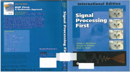
Signal Processing First

Also Available:
International Edition

iiznal Processing Fir;
James H. McClellan
Georgia Institute of Technology
Ronald W. Schafer
Georgia Institute of Technology
Mark A. Yoder
Rose-Hulman Institute of Technology
Pearson Education International

•chased this book within the United States or Canada you should be aware that
n wrongfully imported without the approval of the Publisher or Author.
Vice President and Editorial Director, ECS: Marcia Horton
Publisher: Tom Robbins
Editorial Assistant: Eric Van Ostenbridge
Vice President and Director of Production and Manufacturing, ESM: David W. Riccardi
Executive Managing Editor:
Managing Editor: David A. George
Production Editor: Rose Kernan
Vince O 'Brien
Director of Creative Services: Paul Belfanti
Creative Director: Carole Anson
Art Director: Jayne Conte
Art Editor: Gregory Dulles
Cover Designer: Bruce Kenselaar
Manufacturing Manager: Trudy Pisciotti
Manufacturing Buyer: Lisa McDowell
Marketing Manager: Holly Stark
Cat: Percy
Contents
MATLAB is a registered trademark of The MathWorks, Inc. 3 Apple Hill Drive, Natick, MA 07160-2098.
© 2003 by Pearson Education, Inc.
Pearson Prentice Hall
Upper Saddle River, NJ 07458
All rights reserved. No part of this book may be reproduced in any form or by any means, without permission in writing from the publisher.
The author and publisher of this book have used their best efforts in preparing this book. These efforts include the development, research, and
testing of the theories and programs to determine their effectiveness. The author and publisher make no warranty of any kind, expressed or
implied, with regard to these programs or the documentation contained in this book. The author and publisher shall not be liable in any event
for incidental or consequential damages in connection with, or arising out of, the furnishing, performance, or use of these programs.
PREFACE
xiv
Pearson Prentice Hall® is a trademark of Pearson Education, Inc.
Printed in the United States of America
10
ISBN D-13-lEDEb5-D
Pearson Education Ltd.
Pearson Education Australia Pty. Ltd.
Pearson Education Singapore, Pte. Ltd.
Pearson Education North Asia Ltd.
Pearson Education Canada, Inc.
Pearson Education de Mexico, S.A. de C.V.
Pearson Education—Japan
Pearson Education Malaysia, Pte. Ltd.
Pearson Education, Inc., Upper Saddle River, New Jersey
Introduction 1
1 - 1 Mathematical Representation of Signals 2
1-2 Mathematical Representation of Systems 4
1-3 Thinking About Systems 5
1-4 The Next Step 6
Sinusoids 7
2-1 Tuning Fork Experiment 8
2-2 Review of Sine and Cosine Functions 9
2-3 Sinusoidal Signals 1
in

IV
CONTENTS
CONTENTS
2-3.1 Relation of Frequency to Period 12
2-3.2 Phase Shift and Time Shift 13
2-4 ' Sampling and Plotting Sinusoids 15
2-5 Complex Exponentials and Phasors 17
2-5.1 Review of Complex Numbers 17
2-5.2 Complex Exponential Signals 18
2-5.3 The Rotating Phasor Interpretation 19
2-5.4 Inverse Euler Formulas 21
2-6 Phasor Addition 22
2-6.1 Addition of Complex Numbers 23
2-6.2 Phasor Addition Rule 23
2-6.3 Phasor Addition Rule: Example 24
2-6.4 MATLAB Demo of Phasors 25
2-6.5 Summary of the Phasor Addition Rule 26
2-7 Physics of the Tuning Fork 27
2-7.1 Equations from Laws of Physics 27
2-7.2 General Solution to the Differential Equation 29
2-7.3 Listening to Tones 29
2-8 Time Signals: More Than Formulas 29
2-9 Summary and Links 30
2-10 Problems 31
Spectrum Representation 36
3-1 The Spectrum of a Sum of Sinusoids 36
3-1.1 Notation Change 38
3-1.2 Graphical Plot of the Spectrum 38
3-2 Beat Notes 39
3-2.1 Multiplication of Sinusoids 39
3-2.2 Beat Note Waveform 40
3-2.3 Amplitude Modulation 41
3-3 Periodic Waveforms 43
3-3.1 Synthetic Vowel 44
3-3.2 Example of a Nonperiodic Signal 45
3-4 Fourier Series .
47
3-4.1 Fourier Series: Analysis 48
3-4.2 Fourier Series Derivation 48
3-5 Spectrum of the Fourier Series 50
3-6
3-7
3-8
3-9
3-10
Fourier Analysis of Periodic Signals 51
3-6.1 The Square Wave 52
3-6.1.1 DC Value of a Square Wave 53
3-6.2 Spectrum for a Square Wave 53
3-6.3 Synthesis of a Square Wave 54
3-6.4 Triangle Wave 55
3-6.5 Synthesis of a Triangle Wave 56
3-6.6 Convergence of Fourier Synthesis 57
Time-Frequency Spectrum 57
3-7.1 Stepped Frequency 59
3-7.2 Spectrogram Analysis 59
Frequency Modulation: Chirp Signals 60
3-8.1 Chirp or Linearly Swept Frequency 60
3-8.2 A Closer Look at Instantaneous Frequency 62
Summary and Links 63
Problems 64
4 Sampling and Aliasing 71
4-1 Sampling 71
4-1.1 Sampling Sinusoidal Signals 73
4-1.2 The Concept of Aliasing 75
4-1.3 Spectrum of a Discrete-Time Signal 76
4-1.4 The Sampling Theorem 77
4-1.5 Ideal Reconstruction 78
4-2 Spectrum View of Sampling and Reconstruction 79
4-2.1 Spectrum of a Discrete-Time Signal Obtained by Sampling 79
4-2.2 Over-Sampling 79
4-2.3 Aliasing Due to Under-Sampling 81
4-2.4 Folding Due to Under-Sampling 82
4-2.5 Maximum Reconstructed Frequency 83
88
,
4-3 Strobe Demonstration 84
4-3.1 Spectrum Interpretation 87
4-4 Discrete-to-Continuous Conversion 88
4-4.1 Interpolation with Pulses
4-4.2 Zero-Order Hold Interpolation 89
4-4.3 Linear Interpolation 90

VI
CONTENTS
CONTENTS
vn
4-4.4 Cubic Spline Interpolation 90
4-4.5 Over-Sampling Aids Interpolation 91
4-4.6 Ideal Bandlimited Interpolation 92
4-5 The Sampling Theorem 93
4-6 Summary and Links 94
4-7 Problems 96
FIR Filters 101
5-1 Discrete-Time Systems 102
5-2 The Running-Average Filter 102
5-3 The General FIR Filter 105
5-3.1 An Illustration of FIR Filtering 106
5-3.2 The Unit Impulse Response 107
5-3.2.1 Unit Impulse Sequence 107
5-3.2.2 Unit Impulse Response Sequence 108
5-3.2.3 The Unit-Delay System 109
5-3.3 Convolution and FIR Filters 110
5-3.3.1 Computing the Output of a Convolution 110
5-3.3.2 Convolution in MATLAB Ill
5-4 Implementation of FIR Filters Ill
5-4.1 Building Blocks Ill
5-4.1.1 Multiplier 112
5-4.1.2 Adder 112
5-4.1.3 Unit Delay 112
5-4.2 Block Diagrams 113
5-4.2.1 Other Block Diagrams 113
5-4.2.2 Internal Hardware Details 115
5-5 Linear Time-Invariant (LTI) Systems 115
5-5.1 Time Invariance 116
5-5.2 Linearity 117
5-5.3 The FIR Case 117
5-6 Convolution and LTI Systems 118
5-6.1 Derivation of the Convolution Sum 118
5-6.2 Some Properties of LTI Systems 120
5-6.2.1 Convolution as an Operator 121
5-6.2.2 Commutative Property of Convolution 121
5-6.2.3 Associative Property of Convolution 121
5-7 Cascaded LTI Systems 122
5-8 Example of FIR Filtering 124
5-9 Summary and Links 126
5-10 Problems 126
6 Frequency Response of FIR Filters 130
6-1 Sinusoidal Response of FIR Systems 130
6-2 Superposition and the Frequency Response 1 32
6-3 Steady-State and Transient Response 135
6-4 Properties of the Frequency Response 1 37
6-4.1 Relation to Impulse Response and Difference Equation 137
6-4.2 Periodicity of H(e J& )
138
6-4.3 Conjugate Symmetry 138
6-5 Graphical Representation of the Frequency Response 139
6-5.1 Delay System 139
6-5.2 First-Difference System 140
6-5.3 A Simple Lowpass Filter 142
6-6 Cascaded LTI Systems 143
6-7 Running-Average Filtering 145
6-7.1 Plotting the Frequency Response 146
6-7.2 Cascade of Magnitude and Phase 148
6-7.3 Experiment: Smoothing an Image 149
6-8 Filtering Sampled Continuous-Time Signals 151
6-8.1 Example: Lowpass Averager 152
6-8.2 Interpretation of Delay 154
6-9 Summary and Links 155
6-10 Problems 157
z-Transforms 163
7-1 Definition of the z-Transform 164
7-2 The z-Transform and Linear Systems 165
7-2.1 The z-Transform of an FIR Filter 166

Vlll
CONTENTS
CONTENTS
IX
8
7-3 Properties of the z-Transform
7-3.1 The Superposition Property of the z-Transform 168
7-3.2 The Time-Delay Property of the z -Transform 168
7-3.3 A General z-Transform Formula I69
7-4 The z-Transform as an Operator
7-4.1 Unit-Delay Operator
7-4.2 Operator Notation
7-4.3 Operator Notation in Block Diagrams 170
7-5 Convolution and the z-Transform
7-5.1 Cascading Systems
7-5.2 Factoring z-Polynomials
7-5.3 Deconvolution
7-6 Relationship Between the z-Domain and the co-Domain 175
7-6.1 The z-Plane and the Unit Circle 176
7-6.2 The Zeros and Poles of H(z) 177
7-6.3 Significance of the Zeros of H(z) 178
7-6.4 Nulling Filters
7-6.5 Graphical Relation Between z and to
1 80
7-7 Useful Filters 101
7-7.1 The L-Point Running-Sum Filter
7-7.2 A Complex Bandpass Filter
7-7.3 A Bandpass Filter with Real Coefficients 185
7-8 Practical Bandpass Filter Design
7-9 Properties of Linear-Phase Filters
7-9.1 The Linear-Phase Condition 189
7-9.2 Locations of the Zeros of FIR Linear-Phase Systems 189
7-10 Summary and Links joq
7-11 Problems iq,
IIR Filters
196
8-1 The General IIR Difference Equation 197
8-2 Time-Domain Response mo
8-2.1 Linearity and Time Invariance of IIR Filters 199
8-2.2 Impulse Response of a First-Order IIR System 200
8-2.3 Response to Finite-Length Inputs 201
8-2.4 Step Response of a First-Order Recursive System 202
8-3 System Function of an IIR Filter
8-3.1 The General First-Order Case 205
157
1 69
I69
17Q
171
173
174
175
179
181
I83
186
I89
204
8-3.2 The System Function and Block-Diagram Structures 206
8-3.2.1 Direct Form I Structure 206
8-3.2.2 Direct Form II Structure 207
8-3.2.3 The Transposed Form Structure 208
8-3.3 Relation to the Impulse Response 209
8-3.4 Summary of the Method 209
8-4 Poles and Zeros 210
8-4.1 Poles or Zeros at the Origin or Infinity 211
8-4.2 Pole Locations and Stability 211
8-5 Frequency Response of an IIR Filter 212
8-5.1 Frequency Response using MATLAB 213
8-5.2 Three-Dimensional Plot of a System Function 214
8-6 Three Domains 216
8-7 The Inverse z-Transform and Some Applications 216
8-7.1 Revisiting the Step Response of a First-Order System 217
8-7.2 A General Procedure for Inverse z -Transformation 218
8-8 Steady-State Response and Stability 220
8-9 Second-Order Filters 223
8-9.1 z-Transform of Second-Order Filters 223
8-9.2 Structures for Second-Order IIR Systems 224
8-9.3 Poles and Zeros 225
8-9.4 Impulse Response of a Second-Order IIR System 226
8-9.4.1 Real Poles 227
8-9.5 Complex Poles 228
8-10 Frequency Response of Second-Order IIR Filter 231
8-10.1 Frequency Response via MATLAB 232
8-10.2 3-dB Bandwidth 232
8-10.3 Three-Dimensional Plot of System Functions 233
8-11 Example of an IIR Lowpass Filter 236
8-12 Summary and Links 237
8-13 Problems 238
Continuous-Time Signals and LTI Systems 245
9-1 Continuous-Time Signals 246
9-1.1 Two-Sided Infinite-Length Signals 246
9-1.2 One-Sided Signals 247
9-1.3 Finite-Length Signals 248

CONTENTS
CONTENTS
XI
9-2 The Unit Impulse 248
9-2. 1 Sampling Property of the Impulse 250
9-2.2 Mathematical Rigor 252
9-2.3 Engineering Reality 252
9-2.4 Derivative of the Unit Step 252
9-3 Continuous-Time Systems 254
9-3.1 Some Basic Continuous-Time Systems 254
9-3.2 Continuous-Time Outputs 255
9-3.3 Analogous Discrete-Time Systems 255
9-4 Linear Time-Invariant Systems 255
9-4.1 Time-Invariance 256
9-4.2 Linearity 256
9-4.3 The Convolution Integral 257
9-4.4 Properties of Convolution 259
9-5 Impulse Responses of Basic LTI Systems 260
9-5.1 Integrator 260
9-5.2 Differentiator 261
9-5.3 Ideal Delay 261
9-6 Convolution of Impulses 261
9-7 Evaluating Convolution Integrals 263
9-7.1 Delayed Unit-Step Input 263
9-7.2 Evaluation of Discrete Convolution 267
9-7.3 Square-Pulse Input 268
9-7.4 Very Narrow Square Pulse Input 269
9-7.5 Discussion of Convolution Examples 270
9-8 Properties of LTI Systems 270
9-8.1 Cascade and Parallel Combinations 270
9-8.2 Differentiation and Integration of Convolution 272
9-8.3 Stability and Causality 273
9-9 Using Convolution to Remove Multipath Distortion 276
9-10 Summary 278
9-11 Problems 279
Frequency Response 285
10-1 The Frequency Response Function for LTI Systems 285
10-1.1 Plotting the Frequency Response 287
10-1.1.1 Logarithmic Plot 288
10-1.2 Magnitude and Phase Changes 288
10-2 Response to Real Sinusoidal Signals 289
10-2.1 Cosine Inputs 290
10-2.2 Symmetry of H{ja)) 290
10-2.3 Response to a General Sum of Sinusoids 293
10-2.4 Periodic Input Signals 294
10-3 Ideal Filters 295
10-3.1 Ideal Delay System 295
10-3.2 Ideal Lowpass Filter 296
10-3.3 Ideal Highpass Filter
297
10-3.4 Ideal Bandpass Filter 297
10-4 Application of Ideal Filters 298
10-5 Time-Domain or Frequency-Domain? 300
10-6 Summary/Future ^01
10-7 Problems
11 Continuous-Time Fourier Transform 307
11-1 Definition of the Fourier Transform 308
11-2 Fourier Transform and the Spectrum 310
11-2.1 Limit of the Fourier Series 310
11-3 Existence and Convergence of the Fourier Transform 312
11-4 Examples of Fourier Transform Pairs 313
11-4.1 Right- Sided Real Exponential Signals 313
11-4.1.1 Bandwidth and Decay Rate 314
11-4.2 Rectangular Pulse Signals 314
11-4.3 Bandlimited Signals 316
11-4.4 Impulse in Time or Frequency 317
11-4.5 Sinusoids
11-4.6 Periodic Signals 319
11-5 Properties of Fourier Transform Pairs 322
11-5.1 The Scaling Property 322
11-5.2 Symmetry Properties of Fourier Transform Pairs 324
11-6 The Convolution Property 326
11-6.1 Frequency Response 326
11-6.2 Fourier Transform of a Convolution 327
11-6.3 Examples of the Use of the Convolution Property 328
11-6.3.1 Convolution of Two Bandlimited Functions 328
11-6.3.2 Product of Two Sine Functions 329
11-6.3.3 Partial Fraction Expansions 330
302
318

Xll
CONTENTS
CONTENTS
x.111
11-7
11-8
11-9
11-10
11-11
11-12
Basic LTI Systems
11-7.1 Time Delay
1 1-7.2 Differentiation
11-7.3 Systems Described by Differential Equations 334
The Multiplication Property
11-8.1 The General Signal Multiplication Property 335
11-8.2 The Frequency Shifting Property 335
Table of Fourier Transform Properties and Pairs 337
Using the Fourier Transform for Multipath Analysis 337
Summary
341
Problems
12 Filtering, Modulation, and Sampling 346
12-1
12-2
12-3
12-4
12-5
Linear Time-Invariant Systems
12-1.1 Cascade and Parallel Configurations 347
12-1.2 Ideal Delay 340
12-1.3 Frequency Selective Filters 351
12-1.3.1 Ideal Lowpass Filter 351
12-1.3.2 Other Ideal Frequency Selective Filters
352
12-1.4 Example of Filtering in the Frequency-Domain 353
12-1.5 Compensation for the Effect of an LTI Filter
355
Sinewave Amplitude Modulation
12-2.1 Double-Sideband Amplitude Modulation 353
12-2.2 DSBAM with Transmitted Carrier (DSBAM-TC) 362
12-2.3 Frequency Division Multiplexing
Sampling and Reconstruction
12-3.1 The Sampling Theorem and Aliasing 353
12-3.2 Bandlimited Signal Reconstruction
12-3.3 Bandlimited Interpolation
12-3.4 Ideal C-to-D and D-to-C Converters 373
12-3.5 The Discrete-Time Fourier Transform
375
12-3.6 The Inverse DTFT .2,16
12-3.7 Discrete-Time Filtering of Continuous-Time Signals 377
Summary .
Problems 30,
339
332
333
335
342
34^
35g
355
3^g
370
372
13 Computing the Spectrum 389
13-1 Finite Fourier Sum 390
13-2 Too Many Fourier Transforms? 391
13-2.1 Relation of the DTFT to the CTFT 392
13-2.2 Relation of the DFT to the DTFT 393
13-2.3 Relation of the DFT to the CTFT 393
13-3 Time-Windowing 393
13-4 Analysis of a Sum of Sinusoids 395
13-4.1 DTFT of a Windowed Sinusoid 398
13-5 Discrete Fourier Transform 399
13-5.1 The Inverse DFT 400
13-5.2 Summary of the DFT Representation 401
13-5.3 The Fast Fourier Transform (FFT) 402
13-5.4 Negative Frequencies and the DFT 402
13-5.5 DFT Example 403
13-6 Spectrum Analysis of Finite-Length Signals 405
13-7 Spectrum Analysis of Periodic Signals 407
13-8 The Spectrogram 408
13-8.1 Spectrogram Display 409
13-8.2 Spectrograms in MATLAB 410
13-8.3 Spectrogram of a Sampled Periodic Signal 410
13-8.4 Resolution of the Spectrogram 411
13-8.4.1 Resolution Experiment 412
13-8.5 Spectrogram of a Musical Scale 413
13-8.6 Spectrogram of a Speech Signal 415
13-8.7 Filtered Speech 418
13-9 The Fast Fourier Transform (FFT) 420
13-9.1 Derivation of the FFT 420
13-9.1.1 FFT Operation Count 421
13-10 Summary and Links 423
13-11 Problems 424
Complex Numbers 427
A-l Introduction 428
A-2 Notation for Complex Numbers 428
A-2.1 Rectangular Form 428

XIV
CONTENTS
CONTENTS
xv
A-3
A-4
A-5
A-6
A-7
A-8
A-2.2 Polar Form 429
A-2.3 Conversion: Rectangular and Polar 430
A-2.4 Difficulty in Second or Third Quadrant 431
Euler's Formula 431
A-3.1 Inverse Euler Formulas 432
Algebraic Rules for Complex Numbers 432
A-4.1 Complex Number Exercises 434
Geometric Views of Complex Operations 434
A-5.1 Geometric View of Addition 435
A-5.2 Geometric View of Subtraction 435
A-5.3 Geometric View of Multiplication 437
A-5 .4 Geometric View of Division 437
A-5. 5 Geometric View of the Inverse, z~ l 437
A-5.6 Geometric View of the Conjugate, z* 438
Powers and Roots 433
A-6.1 Roots of Unity 439
A-6. 1.1 Procedure for Finding Multiple Roots 440
Summary and Links 44]
Problems 441
B Programming in MATLAB 443
B-l MATLAB Help 444
B-2 Matrix Operations and Variables 444
B-2.1 The Colon Operator 445
B-2.2 Matrix and Array Operations 445
B-2.2.1 A Review of Matrix Multiplication 445
B-2.2. 2 Pointwise Array Operations 446
B-3 Plots and Graphics 445
B-3.1 Figure Windows 447
B-3.2 Multiple Plots 447
B-3.3 Printing and Saving Graphics 447
B-4 Programming Constructs 447
B-4.1 MATLAB Built-in Functions 448
B-4.2 Program Flow 443
B-5 MATLAB Scripts 443
B-6 Writing a MATLAB Function 448
B-6.1 Creating A Clip Function 449
B-6.2 Debugging a MATLAB M-file 451
B-7 Programming Tips 451
B-7.1 Avoiding Loops 452
B-7.2 Repeating Rows or Columns 452
B-7.3 Vectorizing Logical Operations 452
B-7.4 Creating an Impulse 453
B-7.5 The Find Function 453
B-7.6 Seek to Vectorize 454
B-7.7 Programming Style 454
C Laboratory Projects 455
C-l Introduction to MATLAB 457
C-l.l Pre-Lab 457
C-l. 1.1 Overview 457
C-l. 1.2 Movies: MATLAB Tutorials 457
C-l. 1.3 Getting Started 458
C-1.2 Warm-up 458
C-l.2.1 MATLAB Array Indexing 459
C-l.2.2 MATLAB Script Files 459
C-l.2.3 MATLAB Sound (optional) 460
C-l.3 Laboratory: Manipulating Sinusoids with MATLAB 460
C-l.3.1 Theoretical Calculations 461
C-l.3.2 Complex Amplitude 461
C-l.4 Lab Review Questions 461
C-2 Encoding and Decoding Touch-Tone Signals 463
C-2.1 Introduction 463
C-2.1.1 Review 463
C-2. 1.2 Background: Telephone Touch-Tone Dialing 463
C-2.1.3 DTMFDecoding 464
C-2.2 Pre-Lab 464
C-2.2.1 Signal Concatenation 464
C-2.2. 2 Comment on Efficiency 465
C-2.2.3 Encoding from a Table 465
C-2.2.4 Overlay Plotting 465

XVI
CONTENTS
C-2.3 Warm-up: DTMF Synthesis 465
C-2.3.1 DTMF Dial Function 466
C-2.3.2 Simple Bandpass Filter Design 467
C-2.4 Lab: DTMF Decoding 468
C-2.4.1 Filter Bank Design: dtmfdesign. m 468
C-2.4.2 A Scoring Function: dtmf score, m 469
C-2.4.3 DTMF Decode Function: dtmfrun. m 470
C-2.4.4 Testing 471
C-2.4.5 Telephone Numbers 471
C-2.4.6 Demo 472
C-3 Two Convolution GUIs 473
C-3.1 Introduction 473
C-3.2 Pre-Lab: Run the GUIs 473
C-3. 2.1 Discrete-Time Convolution Demo 473
C-3. 2.2 Continuous-Time Convolution Demo 474
C-3.3 Warm-up: Run the GUIs 475
C-3. 3.1 Continuous-Time Convolution GUI 475
C-3.3.2 Discrete Convolution GUI 475
C-3.4 Lab Exercises 475
C-3.4.1 Continuous-Time Convolution 475
C-3.4.2 Continuous-Time Convolution Again 476
C-3.4. 3 Discrete-Time Convolution 476
D CD-ROM Demos
Index
482
478
This book and its accompanying CD-ROM are the result
of almost 10 years of work that originated from, and
was guided by, the premise that signal processing is
the best starting point for the study of both electrical
engineering and computer engineering.
of 1993, two of us (J.
In the summer
H. McC and R. W. S) began to
develop a one-quarter course that was to become the first
course for Georgia Tech computer engineering students,
who were at that time following an overlapping, but
separate, curriculum track from the electrical engineering
students in the School of ECE. We argued that the
subject of digital signal processing (DSP) had everything
we wanted in a first course for computer engineers: it
introduced the students to the use of mathematics as
a language for thinking about engineering problems; it
laid useful groundwork for subsequent courses; it made
a strong connection to digital computation as a means for
implementing systems; and it offered the possibility of
interesting applications to motivate beginning engineers
to do the hard work of connecting mathematics and
computation to problem solving.
ff;
We were not the first to have this idea.
In particular,
two books by Professor Ken Steiglitz of Princeton
University had a major impact on our thinking. 1
The
major reasons that it was feasible in 1993 to experiment
with what came to be known at
Georgia Tech as the
"DSP First" approach were: (1) the easy accessibility
of increasingly powerful personal computers and (2) the
availability
of MATLAB, a powerful and easy-to-use
software environment for numerical computation.
Indeed, Steiglitz' s 1972 book was well ahead of its
time, since DSP had few practical applications, and even
simple simulations on then-available batch processing
computers required significant programming effort.
the early 1990s, however, DSP applications such as
CD audio, high-speed modems, and cell phones were
widespread due to the availability of low-cost "DSP
chips" that could perform extensive computation in
By
l
An Introduction to Discrete Systems, John Wiley & Sons, 1972,
and A Digital Signal Processing Primer: With Applications to
Computer Music, Addison-Wesley Publishing Company, 1 996.
XVll

XV111
PREFACE
PREFACE
xix
"real time." Thus, integrated circuit technology was
the driving force that simultaneously provided the
wherewithal both for a convenient PC-based laboratory
experience for learning DSP and for creating a climate
of applications that provided motivation for that study.
From the beginning, we believed that "hands-on"
experience with real signals was crucial. This is
provided by a "laboratory" based on MATLAB running
on PCs.
In the laboratory assignments, students gain
direct reinforcement from hearing and seeing the effects
of filtering
operations that they have implemented on
sound and image signals.
sinusoids,
They synthesize music from
and they see that those same sinusoids are
the basis for the data modems that they use routinely to
access the Internet.
it
We also found that MATLAB made
possible to quickly develop demonstration programs
for visualizing and clarifying complicated mathematical
concepts.
By 1 995, we had written notes covering the
topics in our course, and we had amassed a large amount
of computer-based supporting material.
Mark Yoder,
while on sabbatical leave from Rose-Hulman, had the
idea to put all of this material in a form that other teachers
(and students) could access easily. That idea led to a CD-
ROM that captured the entire contents of our course web
site. It included demonstrations and animations used in
classes, laboratory assignments, and solved homework
problems. As teachers, this material has changed the way
we present ideas, because it offers new ways to visualize a
concept "beyond the equations." Over the years, our web
site has continued to grow. We anticipate that this growth
will continue, and that users of this material will see new
ideas take shape in the form of additional demos and labs.
In 1998, all of this material was packaged together in a
textbook/CD-ROM, and we gave it the descriptive title
DSP First: A Multimedia Approach.
No sooner had we finished DSP First,
then Georgia
Tech switched from a quarterly system to semesters,
and our expanded course became "Signal Processing
First," the first course for computer engineers and
electrical engineers. However, we found ourselves
with a textbook that only covered two-thirds of the
material that we needed to include for the semesterlong,
required signals and systems core course in
our semester curriculum. 2 This led to another four
years of development that included four new chapters
on continuous-time signal processing and the Fourier
transform;
such as filtering,
many new laboratory assignments in areas
Fourier series, and analog and digital
communications; many new demos and visualizations;
hundreds of new homework problems and solutions; and
updates of many of our original computer demos.
The present text is our effort to implement an expanded
version of our basic philosophy. It is a conventional book,
although, as our title Signal Processing First suggests, the
distinguishing feature of the text (and the accompanying
CD-ROM) is that it presents signal processing at a level
consistent with an introductory ECE course, i.e., the
sophomore level in a typical U.S. university.
The list
of topics in the book is not surprising, but since we
must combine signal processing concepts with some
introductory ideas, the progression of topics may strike
some teachers as unconventional.
Part of the reason
for this is that in the electrical engineering curriculum,
signals and systems and DSP typically have been treated
as junior- and senior-level courses, for which a traditional
background of linear circuits and linear systems is
assumed. We continue to believe strongly that there are
compelling reasons for turning this order around, since
the early study of signal processing affords a perfect
opportunity to show electrical and computer engineering
students that mathematics and digital computation
can be the key to understanding familiar engineering
applications. Furthermore, this approach makes the
subject much more accessible to students in other
2 DSP First, which remains in print, is still appropriate for a
quarter-length course or for a "signal processing lite" course in non-
ECE fields. This book is currently under revision along the lines of
changes in Chapters 1-8 of Signal Processing First.
majors such as computer science and other engineering
fields.
This point is increasingly important because nonspecialists
are beginning to use DSP techniques routinely
in many areas of science and technology.
Signal Processing First is organized to move from
simple continuous-time sinusoidal signals,
to discretetime
signals and systems, then back to continuoustime,
and finally, the discrete and continuous are
mixed together as they often are in real engineering
systems. A look at the table of contents shows that
the book begins very simply (Chapter 2) with a detailed
discussion of continuous-time sinusoidal signals and
their representation by complex exponentials.
This is a
topic traditionally introduced in a linear circuits course.
We then proceed to introduce the spectrum concept
(Chapter 3) by considering sums of sinusoidal
signals
with a brief introduction to Fourier series. At this
point we make the transition to discrete-time signals by
considering sampled sinusoidal signals (Chapter 4). This
allows us to introduce the important issues in sampling
without the additional complexity of Fourier transforms.
Up to this point in the text, we have only relied on the
simple mathematics of sine and cosine functions.
The
basic linear system concepts are then introduced with
simple FIR filters (Chapter 5). The key concept of
frequency response is
filters (Chapter 6),
derived and interpreted for FIR
and then we introduce ^-transforms
(Chapter 7) and IIR systems (Chapter 8).
The first eight
chapters are very similar to the those ofDSP First. At this
point, we return to continuous-time signals and systems
with the introduction of convolution integrals (Chapter 9)
and then frequency response for continuous-time systems
(Chapter 10). This leads naturally to a discussion of
the Fourier transform as a general representation of
continuous-time signals (Chapter 11). The last two
chapters of the book cap off the text with discussions
of applications of the concepts discussed in the early
chapters. At this stage, a student who has faithfully
read the text, worked homework problems, and done the
laboratory assignments related to the early chapters will
be rewarded with the ability to understand applications
involving linear filtering, amplitude modulation, the
sampling theorem and discrete-time filtering, and
spectrum analysis.
At Georgia Tech, our sophomore-level, 15-week
course covers most of the content of Chapters 2-12
in a format involving two one-hour lectures, one 1.5
hour recitation, and one 1.5 hour laboratory period per
week. As mentioned previously, we place considerable
emphasis on the lab because we believe that it is essential
for motivating our students to learn the mathematics of
signal processing, and because it introduces our students
to the use of powerful software in engineering analysis
and design. At Rose-Hulman, we use Signal Processing
First in a junior-level, 10-week course that covers
Chapters 4-13. The Rose format is four one-hour lectures
per week.
The students use MATLAB throughout the
course, but do not have a separate laboratory period.
As can be seen from the previous discussion, Signal
Processing First is not a conventional signals and systems
book. One difference is the inclusion of a significant
amount of material on sinusoids and complex phasor
representations. In a traditional electrical engineering
curriculum, these basic notions are covered under the
umbrella of linear circuits taken before studying signals
and systems. Indeed, our choice of title for this book
and its ancestor is designed to emphasize this departure
from tradition. An important point is that teaching
signal processing first also opens up new approaches
to teaching linear circuits, since there is much to build
upon that will allow redirected emphasis in the circuits
course. At Georgia Tech, we use the fact that students
have already seen phasors and sinusoidal steady-state
response to move more quickly from resistive circuits
to AC circuits. Furthermore, students have also seen the
important concepts of frequency response and poles and
zeros before studying linear circuits. This allows more
emphasis on circuits as linear systems. For example, the

XX
PREFACE
PREFACE
xxi
Laplace transform is used in the circuits course as a tool
for solving the particular systems problems associated
with linear circuits.
This has resulted in a new textbook
with accompanying CD-ROM co-authored by Professors
Russell Mersereau and Joel Jackson. 3
A second difference from conventional signals and
systems texts is that Signal Processing First emphasizes
topics that rely on "frequency domain" concepts.
This
means that topics like Laplace transforms, state space,
and feedback control, are absent. At Georgia Tech,
these topics are covered in the required linear circuits
course and in a junior-level "tier two" course on control
systems.
Although our text has clearly been shaped by
a specific point of view, this does not mean that it and
the associated CD-ROM can only be used in the way
that they are used at Georgia Tech. For example, at
Rose-Hulman the material on sinusoids and phasors is
skipped in a junior-level course because students have
already had this material in a circuits course. This allows
us to cover the latter part of the text in one quarter.
Indeed, by appropriate selection of topics, our text can
be used for either a one-quarter or one-semester signals
and systems course that emphasizes communications
and signal processing applications from the frequency
domain point of view.
For most electrical engineering
curricula, the control-oriented topics would have to be
covered elsewhere. In other curricula, such as computer
science and computer engineering,
Signal Processing
First emphasizes those topics that are most relevant to
multimedia computing, and the control -oriented topics
are generally not a required part of the curriculum. This is
also likely to be true in other engineering fields where data
acquisition and frequency domain analysis is assuming a
prominent role in engineering analysis and design. 4
3 R. M. Mersereau and J. R. Jackson, Circuits; A Systems
Perspective, to be published by Pearson Prentice Hall, Pearson
Education, Inc.
4 Note that the latter chapters of Signal Processing First require a
calculus background. On the other hand, DSP First does not.
The CD-ROM that accompanies the present text
contains all of the material that we currently use in
teaching our one-semester first
course for sophomore
electrical and computer engineering students. This
type of material has become a common supplement for
lecturing in an age where "computers in education" is the
buzz word.
These new forms of computer-based media
provide powerful ways to
express ideas that motivate
our students in their engineering education. As authors,
we continue to experiment with different modes of
presentation, such as the narrations and movies on the
accompanying CD-ROM, along with the huge archive
of solved problems. In the original DSP First CD-
ROM we noticed that finding material was a challenge,
so we have provided a search engine on this CD-ROM
in order to make is
keywords searches.
easy to find relevant material from
Now, for example, if you want to
know why f irfi.lt , mis in the SP-First Toolbox, you
can just search for f irf ilt .m and see all the labs and
homework that use it.
This text and its
associated CD-ROM represents an
untold amount of work by the three authors and many
students and colleagues. Fortunately, we have been able
to motivate a number of extremely talented students to
contribute to this project. Of the many participants,
five students who served as award-winning teaching
assistants over many terms provided essential material
to the CD-ROM. Jeff Schodorf developed the original
aliasing and reconstruction demos for Chapter 4, and did
much of the early organization of all the DSP First CD-
ROM demos along with Mark Yoder. David Anderson
apprenticed with Jeff and then took over the course as its
primary TA. David contributed new labs and redesigned
the DSP First lab format so that the CD-ROM version
would be easy to use.
Jordan Rosenthal developed a
consistent way to write GUIs that has now been used
in all of our demonstrations. Many other students have
benefited from his extraordinary MATLAB expertise.
Greg Krudysz wrote the CON2DIS demo and has now
taken over the primary role in developing GUIs.
In addition, many undergraduates have implemented
MATLAB programs, graphical user interfaces (GUIs),
and demos that are an important part of this CD-ROM.
Most notably, Craig Ulmer developed PeZ as a multiyear
undergraduate research project and contributed
some of the other GUIs used in the labs. Koon Kong
overhauled PeZ for later versions of MATLAB. Joseph
Stanley made our first movie, the tuning fork movie.
Amer Abufadel developed the image filtering demo
for Chapter 6. Emily Eaton wrote the Music GUI
and provided many of the musical scores and piano
performances needed for the songs in the labs.
Rajbabu
Velmurugan improved the Music GUI and provided last
minute updates for all the GUIs labs.
Janak Patel wrote
most of help files for the GUIs. Greg Slabaugh wrote the
Fourier series demo as a JAVA applet,
and Mustayeen
Nayeem converted it into the MATLAB Fourier series
demo. Budyanto Junus wrote the first LTI demo. Mehdi
Javaramand developed parts of the Phasor Races
GUI. Sam Li has participated in the development of
many parts of the labs. He, Arthur Hinson, and Ghassan
Al-Regib also developed many questions for the pre-labs
and warm-ups in the labs. Kathy Harrington created
lists of keywords for searching homework problems and
edited an extensive set of frequently asked questions
for the labs. Bob Paterno recorded a large number of
tutorial movies about MATLAB.
During the past few years many professors have
participated in the sophomore course ECE-2025 at
Georgia Tech as lecturers and recitation instructors.
Many of them have also written problem solutions that
are included on this CD-ROM. We an indebted to the
following for permitting us to include their solutions:
Randy Abler, Yucel Altunbasak, John Bordelon, Giorgio
Casinovi, Russ Callen, Kate Cummings, Richard
Dansereau, Steve DeWeerth, Michael Fan, Bruno Frazier,
Faramarz Fekri, Elias Glytsis, Monty Hayes, Bonnie
Heck, Mary Ann Ingram, Paul Hasler, Chuanyi Ji, Aaron
Lanterman, Russell Mersereau, Geofferey Li, Steve
McLaughlin, Mohamed Moad, Bill
Sayle, Mark Smith,
Whit Smith, David Taylor, Erik Verriest, Doug Williams,
Tony Yezzi, and Tong Zhou.
We are also indebted to Wayne Padgett and Bruce
Black, who have taught ECE-280 at Rose-Hulman and
have contributed many good ideas.
We also want to acknowledge the contributions or
our Publisher, Tom Robbins at Pearson Prentice Hall.
Very early on, he bought into the concept of DSP
First and supported and encouraged us at every step
in that project and its continuation. He also arranged
for reviews of the text and the CD-ROM by some
very thoughtful and careful reviewers, including Filson
Glantz, S. Hossein Mousavinezhad, Geoffrey Orsak,
Mitch Wilkes, Robert Strum, James Kaiser, Victor
DeBrunner, Timothy Schultz, and Anna Baraniecki.
Finally, we want to recognize the understanding and
support of our wives (Carolyn McClellan, Dorothy
Schafer, and Sarah Yoder).
Carolyn's photo of the cat
Percy appears on the cover after undergoing some DSP.
They have patiently supported us as this seemingly neverending
project continued to consume energy and time.
Indeed, this project will continue on beyond the present
text and CD-ROM since there are just too many ideas yet
to explore. That is the appeal of the computer-based and
Web-based approach.
It can easily grow to incorporate
the innovative visualizations and experiments that others
will provide.
J. H. McC
R.W.S.
M.A.Y.

C H
«1 T E R
This is a book about signals and systems.
In this age
of multimedia computers, audio and video entertainment
systems, and digital communication systems, it is almost
certain that you, the reader of this text, have formed
some impression of the meaning of the terms signal and
system, and you probably use the terms often in daily
conversation.
It is likely that your usage and understanding of the
terms are correct within some rather broad definitions.
For example, you may think of a signal as "something"
that carries information. Usually, that something is
a pattern of variations of a physical quantity that can
be manipulated, stored, or transmitted by physical
processes. Examples include speech signals, audio
signals, video or image signals, biomedical signals, radar
signals, and seismic signals, to name just a few. An
important point is that signals can take many equivalent
forms or representations.
For example, a speech signal
is produced as an acoustic signal, but it can be converted
to an electrical signal by a microphone, or a pattern of
magnetization on a magnetic tape, or even a string
numbers as in digital audio recording.
The term system may be somewhat more ambiguous
and subject to interpretation. For example, we often use
"system" to refer to a large organization that administers
or implements some process, such as the "Social Security
system" or the "airline transportation system." However,
we will be interested in a much narrower definition that
is very closely linked to signals. More specifically,
a system, for our purposes, is something that can
manipulate, change, record, or transmit signals. For
example, an audio compact disk (CD) recording stores or
represents a music signal as sequence of numbers. A CD
player is a system for converting the numbers stored on
the disk (i.e., the numerical representation of the signal)
to an acoustic signal that we can hear. In general, systems
of

CHAPTER 1 INTRODUCTION
1 - 1 MATHEMATICAL REPRESENTATION OF SIGNALS
operate on signals to produce new signals or new signal
representations.
Our goal in this text is to develop a framework wherein
it is possible to make precise statements about both
signals and systems.
Specifically, we want to show that
mathematics is an appropriate language for describing
and understanding signals and systems. We also want
to show that the representation of signals and systems
by mathematical equations allows us to understand how
signals and systems interact and how we can design and
implement systems that achieve a prescribed purpose.
3
a
c
50
100
-2000
Samples of a Speech Waveform: s[n] = s(nT s )
50 100 150
Sample Index n
200
Figure 1-2: Example of a discrete-time signal that can be
represented by a one-dimensional sequence or function
oo 150
of a discrete variable.
Signal samples are taken from the
1-1 Mathematical Representation of
Signals
Signals are patterns of variations that represent or encode
information. They have a central role in measurement, in
probing other physical systems, in medical technology,
and in telecommunication, to name just a few areas.
Many signals are naturally thought of as a pattern
of variations in time. A good example is a speech
signal, which initially arises as a pattern of changing
air pressure in the vocal tract.
This pattern, of course,
evolves with time, creating what we often call a time
waveform. Figure 1-1 shows a plot of a speech waveform.
In this plot, the vertical axis represents air pressure or
microphone voltage and the horizontal axis represents
time. Notice that there are four plots in the figure
corresponding to four contiguous time segments of the
speech waveform. The second plot is a continuation of
the first,
and so on, with each graph corresponding to a
time interval of 50 milliseconds (msec).
The speech signal in Fig. 1-1 is an example of a
one-dimensional continuous-time signal.
can be represented mathematically as
Such signals
a function of a
single independent variable, which is normally denoted t.
Although in this particular case we cannot write a simple
10 20 30 40 50
Offset Time t (msec)
Figure 1-1: Plot of part of a speech signal. This signal
can be represented as a function of a single (time) variable,
s(r). The shaded region is shown in more detail in Fig. 1-2.
equation that describes the graph of Fig. 1-1 in terms
of familiar mathematical functions, we can nevertheless
associate a function s(t) with the graph. Indeed, the
graph itself can be taken as a definition of the function
that assigns a number s(t) to each instant of time (each
value of t).
Many, if not most, signals originate as continuoustime
signals. However, for a variety of reasons that
will become increasingly obvious as we progress through
this text, it is often desirable to obtain a discretetime
representation of a signal. This can be done by
sampling a continuous-time signal at isolated, equally
spaced points in time. The result is a sequence ofnumbers
that can be represented as a function of an index variable
that takes on only discrete values. This can be represented
mathematically as s[ri] = s(nT s ), where n is an integer;
shaded region of Fig. 1 - 1
i.e., {. . . , —2, —1,0, 1,2,...}, and T s is the sampling
period. 1
This is, of course, exactly what we do when we
plot values of a function on graph paper or on a computer
screen. We cannot evaluate the function at every possible
value of a continuous variable, only at a set of discrete
points.
Intuitively, we know that the closer the spacing
of the points, the more the sequence retains the shape
of the original continuous-variable function. Figure 1-2
shows an example of a short segment of a discrete-time
signal that was derived by sampling the speech waveform
of Fig. 1-1 with a sampling period of T s
= 1/8 msec. In
this case, a vertical line with a dot at the end shows the
location and the size of each of the isolated sequence
values.
While many signals can be thought of as evolving
patterns in time, many other signals are not time-varying
patterns.
For example, an image formed by focusing
light through a lens is a spatial pattern, and thus is
appropriately represented mathematically as a function of
^ote that our convention will be to use parentheses ( ) to
enclose the independent variable of a continuous-variable function,
and square brackets [ 1 to enclose the independent variable of a
discrete- variable function (sequence).
Figure 1-3: Example of a signal that can be represented
by a function of two spatial variables.
two spatial variables. Such a signal would be considered,
in general, as a function of two independent variables;
i.e., a picture might be denoted p(x, y). A photograph is
another example, such as the "gray-scale image" shown
in Fig. 1-3. In this case, the value p(xo, yo) represents
the shade of gray at position (xq, yo) in the image.
Images such as that in Fig. 1-3 are generally
considered to be two-dimensional continuous-variable
signals, since we normally consider space to be a
continuum. However, sampling can likewise be
used to obtain a discrete-variable two-dimensional
signal from a continuous-variable two-dimensional
signal. Such a two-dimensional discrete-variable signal
would be represented by a two-dimensional sequence
or an array of numbers, and would be denoted
p[m,n\ = p(mA x ,nA y ), where both m and n would
take on only integer values, and A x and A v are the
horizontal and vertical sampling periods, respectively.
Two-dimensional functions are appropriate mathematical
representations of still images that do not change
with time; on the other hand, videos are time-varying

4 CHAPTER 1 INTRODUCTION
1-3 THINKING ABOUT SYSTEMS
images that would require a third independent variable
for time; i.e., v(x, y, t). Video signals are intrinsically
three-dimensional, and, depending on the type of video
x(t)
T{x(t)}
y(t) = T{x(t)}
x(t)
Ideal
C-to-D
Converter
x[n] =x(nT s )
system, either two or all three variables may be discrete.
Our purpose in this section has been simply to
introduce the idea that
signals can be represented by
Figure 1-5: Block diagram representation of a
continuous-time system.
mathematical functions. Although we will soon see that
many familiar functions are quite valuable in the study
of signals and systems, we have not even attempted to
demonstrate that fact.
Our sole concern is to make the
connection between functions and signals, and, at this
point, functions simply serve as abstract symbols for
signals.
Thus, for example, now we can refer to "the
speech signal sit)" or "the sampled image p[m,n]."
Although this may not seem highly significant, we will
see in the next section that it is indeed a very important
step toward our goal of using mathematics to describe
signals and systems in a systematic way.
1-2 Mathematical Representation of
Systems
10 20 30
Offset Time t (msec)
Figure 1-4: Output of a squarer system for the speech
signal input of Fig. 1 -1 . The squarer system is defined by
the equation y(t) = [x(t)] 2
signal is the square of the input signal. The mathematical
description of this system is simply
answer is that the system of (1.2) can be approximated
through appropriate connections of electronic circuits.
On the other hand, if the input and output of the system
are both discrete-time signals (sequences of numbers)
related by
y[n] = (x[n]Y (1.3)
then the system would be a discrete-time system.
The
implementation of the discrete-time squarer system
would be trivial; one simply multiplies each discrete
signal value by itself.
In thinking and writing about systems, it is often
useful to have a visual representation of the system. For
this purpose, engineers use block diagrams to represent
operations performed in an implementation of a system
Figure 1-6: Block diagram representation of a sampler.
which simply states that the sampler "takes an
instantaneous snapshot" of the continuous-time input
signal once every T s seconds. Thus, the operation of
sampling fits our definition of a system, and it can be
represented by the block diagram in Fig. 1-6. Often we
will refer to the sampler system as an "ideal continuousto-discrete
converter" or ideal C-to-D converter. In this
case, as in the case of the squarer, the name that we give to
the system is really just a description of what the system
does.
1-3 Thinking About Systems
As we have already suggested, a system is something that
transforms signals into new signals or different signal
representations.
it is useful as a starting point.
This is a rather abstract definition, but
To be more specific, we
say that a one-dimensional continuous-time system takes
an input signal x (t) and produces a corresponding output
signal >'(?).
This can be represented mathematically by
y(t) = T{x(t)} (1.1)
which means that the input signal (waveform, image, etc.)
is operated on by the system (symbolized by the operator
T) to produce the output y(t). While this sounds very
abstract at first, a simple example will show that this need
not be mysterious. Consider a system such that the output
y(t) = [x(t)Y (1.2)
which says that at each time instant the value of the output
is equal to the square of the input signal value at that
same time. Such a system would logically be termed a
"squarer system." Figure 1-4 shows the output of the
squarer for the input of Fig. 1-1. As would be expected
from the properties of the squaring operation, we see
that the output signal is always nonnegative and the large
signal values are emphasized relative to the small signal
values.
The squarer system defined by (1 .2) is an example of
a continuous-time system; i.e., a system whose input
and output are continuous-time signals. Can we build a
physical system that acts like the squarer system? The
and to show the interrelations among the many signals
that may exist in an implementation of a complex system.
An example of the general form of a block diagram is
shown in Fig. 1-5. What this diagram shows is simply
that the signal y(t) is obtained from the signal x(t) by
the operation T{ }.
Another example of a system was suggested earlier
when we discussed the sampling relationship between
continuous-time signals and discrete-time signals.
Therefore, we would define a. sampler as a system whose
input is a continuous-time signal x(t) and whose output
is the corresponding sequence of samples, defined by the
equation
x[n] =x(nT s ) (1-4)
Block diagrams are useful for representing complex
systems in terms of simpler systems,
which are more
easily understood. For example, Fig. 1-7 shows a
block diagram representation of the process of recording
and playback of an audio CD. This block diagram
breaks the operation down into four subsystems.
first operation is A-to-D (analog-to-digital)
The
conversion,
which is a physical approximation to the ideal C-to-
D converter defined in (1.4). An A-to-D converter
produces finite-precision numbers as samples of the input
signal (quantized to a limited number of bits), while the
ideal C-to-D converter produces samples with infinite
precision. For the high-accuracy A-to-D converters used
in
precision audio systems, the difference between an
A-to-D converter and our idealized C-to-D converter is

6
CHAPTER 1
INTRODUCTION
C H A
T E R
Optical
x(t) A-to-D x[n] CD
Disk
Converter
Writer
Optical
Disk
Reader
x[n]
D-to-A
Converter
HO
Figure 1-7: Simplified block diagram for recording and playback of an audio CD.
slight, but the distinction is very important. Only finiteprecision
quantized sample values can be stored in digital
memory of finite size!
Figure 1-7 shows that the output of the A-to-D
then relatively easy to understand. Details of some parts
can be left to experts in other fields who, for example,
can develop more detailed breakdowns of the optical disk
subsystems.
converter is the input to a system that writes the
numbers x[n] onto the optical disc. This is a complex
process, but for our purposes it is sufficient to simply
show it as a single operation. Likewise, the complex
mechanical/optical system for reading the numbers off
the optical disk is shown as a single operation.
Finally,
the conversion of the signal from discrete-time form to
continuous-time (acoustic) form is
shown as a system
called a D-to-A (digital-to-analog) converter. This
system takes finite precision binary numbers in sequence
and fills in a continuous-time function between the
samples. The resulting continuous-time signal could then
be fed to other systems, such as amplifiers, loudspeakers,
and headphones, for conversion to sound.
Systems like the CD audio system are all around us.
Most of the time we do not need to think about how such
systems work, but this example illustrates the value of
thinking about a complex system in a hierarchical form.
In this way, we can first understand the individual parts,
then the relationship among the parts, and finally the
By looking at the CD audio system in
whole system.
this manner, we see that a very important issue is the
conversion from continuous-time to
discrete-time and
back to continuous-time, and we see that it is possible
to consider these operations separately from the other
parts of the system. The effect of connecting the parts is
1-4 The Next Step
The CD audio system is a good example of a discretetime
system. Buried inside the blocks of Fig. 1-7
are many discrete-time subsystems and signals. While
we do not promise to explain all the details of CD
players or any other complex system, we do hope
to establish the foundations for the understanding of
discrete- and continuous-time signals and systems so
that this knowledge can be applied to understanding
components of more complicated systems. In Chapter 2,
we will start at a basic mathematical level and show
how the well-known sine and cosine functions from
trigonometry play a fundamental role in signal and
system theory. Next, we will show how complex numbers
can simplify the algebra of trigonometric functions.
Subsequent chapters will
introduce the concept of the
frequency spectrum of a signal and the concept of
filtering with a linear time-invariant system. By the
end of the book, the diligent reader who has worked
the problems, experienced the demonstrations, and done
the laboratory exercises will be rewarded with a solid
understanding ofmany of the key concepts underlying the
digital multimedia information systems that are rapidly
becoming commonplace.
We begin our discussion by introducing a general class
of signals that are commonly called cosine signals or,
equivalently, sine signals. 1
Collectively, such signals are
called sinusoidal signals or, more concisely, sinusoids.
Although sinusoidal signals have simple mathematical
representations, they are the most basic signals in the
theory of signals and systems, and it is important to
become familiar with their properties. The most general
mathematical formula for a cosine signal is
x(t) = Acos(o>o? + ) (2.1)
where cos(-) denotes the cosine function that is familiar
from the study of trigonometry. When defining a
It is also common to refer to cosine or sine signals as cosine
or sine waves, particularly when referring to acoustic or electrical
signals.
continuous-time signal, we typically use a function
whose independent variable is t, a continuous variable
that represents time. From (2.1) it follows that x(t)
is a mathematical function in which the angle of the
cosine function is,
in turn, a function of the variable t
The parameters A, coq, and are fixed numbers for a
particular cosine signal. Specifically, A is called the
amplitude, a>o the radian frequency, and (J)
the phase
shift of the cosine signal.
Figure 2-1 shows a plot of the continuous-time cosine
signal
x(t) = 10 cos (27r(440)f - 0,4jt)
i.e., A = 10, o) = 2jt(440), and

CHAPTER 2
SINUSOIDS
2-2 REVIEW OF SINE AND COSINE FUNCTIONS
signal produced by the tuning fork.
The microphone
converts the sound into an electrical signal, which in
A-440 Tuning Fork Signal
turn is converted to a sequence of numbers stored in the
computer.
Then these numbers can be plotted on the
computer screen. A typical plot is shown in Fig. 2-3 for
an A-440 tuning fork. In this case, the A-to-D converter
5 10
Time t (msec)
Figure 2-1: Sinusoidal signal generated from the
formula: x(t) = 10cos(27r(440)f - 0.4tt).
20
sampled the output of the microphone at a rate of
5563.6 samples/sec. 2 The upper plot was constructed by
connecting the sample values by straight lines. It appears
that the signal generated by the tuning fork is very much
like the cosine signal of Fig. 2-1.
It oscillates between
10 15
Time t (msec)
Sample Values at 5563.6 Hz
chapter that most features of the sinusoidal
waveform
are directly dependent on the choice of the parameters A,
coq, and 4>.
2-1 Tuning Fork Experiment
One of the reasons that cosine waves are so important
is that many physical systems generate signals that can
be modeled (i.e., represented mathematically) as sine or
cosine functions versus time. Among the most prominent
of these are signals that are audible to humans. The tones
or notes produced by musical instruments are perceived
as different pitches. Although it is an oversimplification
to equate notes to sinusoids and pitch to frequency, the
mathematics of sinusoids is an essential first step to
understanding complicated sound signals.
To provide some motivation for our study of sinusoids,
we will begin by considering a very simple and familiar
system for generating a sinusoidal signal. This system is
a tuning fork, an example of which is shown in Fig. 2-2.
When struck sharply, the tines of the tuning fork vibrate
and emit a "pure" tone. This tone is at a single frequency,
which is usually stamped on the tuning fork. It is common
to find "A^WO" tuning forks, because 440 hertz (Hz) is
the frequency of A above middle C on a musical scale,
and is often used as the reference note for tuning a piano
Figure 2-2: Picture of a tuning fork and a microphone.
and other musical instruments. If you can obtain a tuning
fork, perform the following experiment:
Strike the tuning fork against your knee, and
then hold it close to your ear. You should hear
a distinct "hum" at the frequency designated
for the tuning fork. The sound will persist for
a rather long time if you have struck the tuning
fork properly; however, it is easy to do this
experiment incorrectly. If you hit the tuning
fork sharply on a hard surface such as a table,
you will hear a high pitched metallic "ting"
sound. This is not the characteristic sound that
you are seeking. If you hold the tuning fork
close to your ear, you will hear two tones: The
higher-frequency "ting" will die away rapidly,
and then the lower-frequency "hum" will be
heard.
' -""-
DEMO: Tuning Fork
With a microphone and a computer equipped with an
A-to-D converter, we can make a digital recording of the
symmetric limits of amplitude and it also repeats periodically
with a period of about 2.27 msec (0.00227 sec). As
we will see in Section 2-3.1, this period is proportional
to the reciprocal of co ; i.e., 2jt/ (27t(440)) % 0.00227.
This experiment shows that common physical systems
produce signals whose graphical representations look
very much like cosine signals; i.e., they look very much
like the graphical plots of the mathematical functions
defined in (2.1). Later, in Section 2-7, we will add
further credence to the sinusoidal model for the tuning
fork sound by showing that cosine functions arise as
solutions to the differential
equation that (through the
laws of physics) describes the motion of the tuning fork's
tines.
Before looking at the physics of the tuning fork,
however, we should become more familiar with sinusoids
and sinusoidal signals.
2-2 Review of Sine and Cosine
Functions
Sinusoidal signals are defined in terms of the familiar sine
and cosine functions of trigonometry. A brief review of
the properties of these basic trigonometric functions is
useful, since these properties determine the properties of
sinusoidal signals.
2 This rate is one-quarter of the A-to-D conversion rate on a
Macintosh computer.
12 3
Time t (msec)
Figure 2-3: Recording of an A-440 tuning fork signal
sampled at a sampling rate of 5563.6 samples/sec. The
bottom plot, which consists of the first 3.6 msec taken
from the top plot, shows the individual sample values (as
circles).
The sine and cosine functions are often introduced
and defined through a diagram like Fig. 2-4. The
trigonometric functions sine and cosine take an angle as
their argument. We often think of angles in degrees, but
where sine and cosine functions are concerned, angles
must be dimensionless.
Angles are therefore specified
in radians. If the angle is in the first quadrant
(0 < < tt/2 rad), then the sine of is the length y of
the side of the triangle opposite the angle
divided by the
length r of the hypotenuse of the right triangle. Similarly,
the cosine of
is the ratio of the length of the adjacent
side x to the length of the hypotenuse.
Note that as 6 increases from to 7r/2, cos decreases
from 1 to and sin increases from to 1 . When the

10 CHAPTER 2 SINUSOIDS
2-3 SINUSOIDAL SIGNALS 11
Table 2-1: Basic properties of the sine and cosine functions.
Property
Equation
Equivalence
Periodicity
Evenness of cosine
Oddness of sine sin(— 9) = — sin 9
Zeros of sine
sin 9 = cos(0 - 7r/2) or cos(#) = sin()
A more extensive table of trigonometric identities may
be found in any book on trigonometry or in a book of
mathematical tables.
&& EXERCISE 2.1 :
Use trigonometric identity
#5 to derive an expression for cos 8$ in terms of cos 99,
cos 79, and cos#.
^^ NOTE: Solutions to all Exercises are on the CD
2-3 Sinusoidal Signals
The most general mathematical formula for a sinusoidal
time signal is obtained by making the argument (i.e., the
angle) of the cosine function be a function of t.
following equation gives two equivalent forms:
The
x(t) = A cos(cD r +

12 CHAPTER 2 SINUSOIDS
2-3 SINUSOIDAL SIGNALS 13
(c) a>o is called the radian frequency. Since the
argument of the cosine function must be in radians,
which is dimensionless, the quantity coot must
likewise be dimensionless. Thus, coq must have
units of rad/sec if t has units of sec. Similarly,
/o = o)q/2tt is called the cyclic frequency, and /o
must have units of sec -1 .
-0.02 0.02
Time t (sec)
0.04
(a) Cosine Signal: / = 200 Hz
-10 -5 5 10 15 20
length is a shorter time interval. We have already seen in
(2.4) that this is true because the period of a cosine signal
is the reciprocal of the frequency.
Note that when the
frequency doubles (100 — 200), the period is halved.
This is
an illustration of the general principle that the
higher the frequency, the more rapid the signal waveform
changes with time.
Throughout this book we will see
more examples of the inverse relationship between time
^5& Example 2-1 : Plotting Sinusoids
Figure 2-6: Sinusoidal signal with parameters A = 20,
coo = 2tt(40), /o = 40, and cf> = -0.4*.
(b) Cosine Signal: /
= 100 Hz
and frequency.
Finally, notice that fo = is a perfectly acceptable
value, and when this value is used, the resulting signal is
Figure 2-6 shows a plot of the signal
x(t) = 20 cos(2tt(40)? - 0.4tt) (2.3)
In terms of our definitions,
the signal parameters are
A = 20, co = 2tt(40), f = 40, and = -0.4tt. The
dependence of the signal on the amplitude parameter A
is obvious; its maximum and minimum values are +20
and -20, respectively. The maxima occur at
and the minima at
. .
The time interval
* = ..., -0.02, 0.005, 0.03, . .
. , -0.0325, -0.0075, 0.0175, . .
between successive maxima of the
signal is l//o = 0.025 sec. To understand why the signal
has these properties, we will need to do a bit of analysis.
DEMO: Sinusoids
2-3.1 Relation of Frequency to Period
The sinusoid in Fig. 2-6 is clearly a periodic signal. The
period of the sinusoid, denoted by 7b, is the length of
one cycle of the sinusoid.
In general, the frequency of
the sinusoid determines its period, and the relationship
can be found by examining the following equations:
A cos(coo(t + To) + 4>)
= x(t)
x(t + T )
= A cos(coot -J- (p)
cos(coot + COqTq + 0) = COS ( ' + 4>)
Since the cosine function has a period of 2tt, the equality
above holds for all values of t if
Ct>0
7b = 27T
(27r/o)7b = 2;r
Tn = —
To =
COq
1
/(
(2.4)
Since To is the period of the signal, f = l/To is the
number of periods (cycles) per second. Therefore, cycles
per second is an appropriate unit for fo, and it was in
general use until the 1960s. 4 When dealing with coq,
the unit of radian frequency is rad/sec.
The units of fo
are often more convenient when describing the sinusoid,
because cycles per second naturally define the period.
DEMO: Sine Drill
4 The unit hertz (abbreviated Hz) was adopted in 1933 by the
Electrotechnical Commission in honor of Heinrich Hertz, who first
demonstrated the existence of radio waves.
-5
-5
-10 -5 5 10
(c) Cosine Signal: /o =
Hz
15 20
-10 -5 5 10 15 20
Time t (msec)
Figure 2-7: Cosine signals x(t) = 5cos(2tt/o?) for
several values of :
/ (a) / = 200 Hz; (b) /o = 100 Hz;
(c) f = 0.
It is very important to understand the effect of the
frequency parameter.
several choices of fo in the signal
Figure 2-7 shows this effect for
x(t) = 5cos(27r/b*)
The two plots in Fig. 2-7(a,b) show the effect of changing
/o- As we expect, the waveform shape is similar for both
values of frequency. However, for the higher frequency,
the signal varies more rapidly with time; i.e., the cycle
constant (Fig. 2-7(c)), since 5 cos(27r • • t) = 5 for all
values of t . Thus, the constant signal, often called DC, 5
is, in fact, a sinusoid of zero frequency.
2-3.2 Phase Shift and Time Shift
The phase shift parameter cf) (together with the frequency)
determines the time locations of the maxima and minima
of a cosine wave. To be specific, notice that the sinusoid
(2.2) with = has a positive peak at t = 0. When

14
CHAPTER 2
SINUSOIDS
2-4 SAMPLING AND PLOTTING SINUSOIDS 15
function x\ (f) = s(t - 2). From the definition of s(t), it
follows that x\ (t) is nonzero for
< (t - 2) < 2 2 < / < 4.
Within the time interval [2, 4], the formula for the shifted
signal is:
x l
(t) =
2(t-2)
2

1
16 CHAPTER 2 SINUSOIDS
2-5 COMPLEX EXPONENTIALS AND PHASORS 17
would create a row vector tn of 13 numbers between
-0.035 and 0.025 spaced by the sampling period 0.005,
and a row vector xn of samples of x(t). Then
the Matlab function plot draws the corresponding
points, connecting them with straight line segments.
Constructing the curve between sample points in this
way is called linear interpolation. The solid gray curve
in the upper plot of Fig. 2-9 shows the result of linear
interpolation when the sample spacing is T s
= 0.005.
Intuitively,
we realize that if the points are very close
together, we will see a smooth curve. The important
question is, "How small must we make the sample
spacing, so that the cosine signal can be accurately
reconstructed between samples by linear interpolation?"
A qualitative answer to this question is provided by
Fig. 2-9, which shows plots produced by three different
sampling periods.
Obviously, the sample spacing of T s
= 0.005 is not
sufficiently close to create an accurate plot when the
sample points are connected by straight lines. Note
that sample points are shown as dots in the upper two
plots. 6 With a spacing of T s
= 0.0025, the plot starts to
approximate a cosine, but it is still possible to see places
where it is clear that the points are connected by straight
lines rather than the smooth cosine function. Only in the
lower plot of Fig. 2-9, where the spacing is T s
= 0.0001,
does the sampling spacing become so dense that our eye
can easily see that the curve is a faithful representation
of the cosine function. 7 A precise answer to the question
posed above would require a mathematical definition of
accuracy; our subjective judgment would be too prone to
variability among different observers. However, we learn
from this example that as the sampling period decreases,
more samples are taken across one cycle of the periodic
cosine signal. When T s = 0.005, there are 5 samples per
6 This was achieved by adding a second plot using Matlab's hold
and stem functions.
Here the points are so close together that we cannot show the
discrete samples as individual large dots.
20 r
(a) Samples of Sinusoid: T s
= 0.005 sec
-0.03 -0.02 -0.01 0.01 0.02 0.03 0.04
(b) T s
= 0.0025 sec
-0.03 -0.02 -0.01 0.01 0.02 0.03 0.04
(c) T s
= 0.0001 sec
-20
-0.03 -0.02 -0.01 0.01 0.02 0.03 0.04
Time t (sec)
Figure 2-9: Sampled cosine signals x{nT s ) =
20cos(2Tu(40)nT s -0Ajt) for several values of T s :
(a) T s = 0.005 sec; (b) T s = 0.0025 sec; (c) T s
= 0.0001
sec.
cycle; when T s
= 0.0025 there are 10 samples per cycle;
and when T s
= 0.0001 , there are 250 samples per cycle.
It seems that 1
samples per cycle is not quite enough, and
250 samples per cycle is probably more than necessary,
but, in general, the more samples per cycle, the smoother
and more accurate is the linearly interpolated curve.
The choice of T s
also depends on the frequency of
the cosine signal, because it is the number of samples
per cycle that matters in plotting.
For example, if the
frequency of the cosine signal were 2000 Hz instead of
40 Hz, then a sample spacing of T s
= 0.0001 would
yield only 5 samples per cycle.
The key to accurate
reconstruction is to sample frequently enough so that the
cosine signal does not change very much between sample
points. This will depend directly on the frequency of the
cosine signal.
The problem of plotting a cosine signal from a set of
discrete samples depends on the interpolation method
used.
With Matlab's built-in plotting function, linear
interpolation is used to connect points by straight-line
segments. An insightful question would be; "If a
more sophisticated interpolation method can be used,
how large can the sample spacing be such that the
cosine signal can be reconstructed accurately from the
samples?"
question is
Surprisingly, the theoretical answer to this
that the cosine signal can be reconstructed
exactly from its samples if the sample spacing is less
than half the period, i.e., the average number of samples
per cycle need be only slightly more than two!
Linear
interpolation certainly cannot achieve this result, but, in
Chapter 4,
where we examine the sampling process in
more detail, we will illustrate how this remarkable result
can be achieved.
For now, our observation that smooth
and accurate sinusoidal curves can be reconstructed from
samples if the sampling period is "small enough" will be
adequate for our purposes.
2-5 Complex Exponentials and
Phasors
We have shown that cosine signals are useful mathematical
representations for signals that arise in a
practical setting, and that they are simple to define
and interpret. However, it turns out that the analysis
and manipulation of sinusoidal signals is
often greatly
simplified by dealing with related signals called complex
z = x + jy iprtt {z} jpm{z]
X X °r
(x,y)
y
(a)
ke[z) ?
z = reJ &
y
ip)
me{z]
Figure 2-10: (a) Cartesian and (b) polar representations
of complex numbers in the complex plane.
exponential signals.
unfamiliar and seemingly artificial
Although the introduction of the
concept of complex
exponential signals may at first seem to be making the
problem more difficult, we will soon see the value in
this new representation. Before introducing the complex
exponential signal, we will first review some basic
concepts concerning complex numbers. 8
2-5.1 Review of Complex Numbers
A complex number z is an ordered pair of real numbers.
Complex numbers may be represented by the notation
z = (x, y), where x = d\e{z} is the real part and
v = %m{z] is the imaginary part of z. Electrical
engineers use the symbol j for v— 1 instead of i, so
we can also represent a complex number as z = x + j v.
These two representations are called the Cartesian form
of the complex number. Complex numbers are often
represented as points in a complex plane, where the
real and imaginary parts are the horizontal and vertical
coordinates, respectively, as shown in Fig. 2- 10(a). With
the Cartesian notation and the understanding that any
8 Appendix A provides a more detailed review ofthe fundamentals
of complex numbers. Readers who know the basics of complex
numbers and how to manipulate them can skim Appendix A and
skip to Section 2-5.2.

CHAPTER 2
SINUSOIDS
2-5 COMPLEX EXPONENTIALS AND PHASORS 19
number multiplied by j is included in the imaginary part,
the operations of complex addition, complex subtraction,
complex multiplication, and complex division can be
defined in terms of real operations on the real and
imaginary parts. For example, the sum of two complex
The rZ9 notation is clumsy, and does not lend itself
to ordinary algebraic rules. A much better polar form is
given by using Euler's famous formula for the complex
exponential
representation for the real cosine signal. This is because
we can always write
x(t) = die {Ae i{0K> i+4>) )
= Acos(co t + 0) (2.14)
numbers is defined as the complex number whose real
part is the sum of the real parts and whose imaginary part
is the sum of the imaginary parts.
e j = cos + j sin
<
(2.10)
The Cartesian pair (cos9, sin0) can represent any point
-20
-0.02 -0.01
Time /
0.01 0.02 0.03 0.04
(sec)
In fact, the real part of the complex exponential signal
shown in Fig. 2-11 is identical to the cosine signal
plotted in Fig. 2-6. Although it may seem that we have
Since complex numbers can be represented as points in
a plane, it follows that complex numbers are analogous to
on a circle of radius 1, so a slight generalization of (2. 1
0)
gives a representation valid for any complex number z
20 r
complicated things by first introducing the imaginary
part to obtain the complex exponential signal and then
vectors in a two-dimensional space. This leads to a useful
geometric interpretation of a complex number as a vector,
z = re-i = r cos 9 + jr sin 9 (2.11)
throwing it away by taking only the real part, we will see
that many calculations are simplified by using properties
shown in Fig. 2- 10(b). Vectors have length and direction,
so another way to represent a complex number is thepolar
form in which the complex number is represented by r,
The complex exponential polar form of a complex
number is most convenient when calculating a complex
multiplication or division (see Appendix A for more
-20
-0.02 -0.01 0.01 0.02 0.03 0.04
Time t (sec)
of the exponents. It is possible, for example, to replace all
trigonometric manipulations with algebraic operations
on the exponents.
its vector length, together with 9, its angle with respect
to the real axis. The length of the vector is also called the
magnitude ofz (denoted \z\), and the angle with the real
axis is called the argument of z (denoted argz). This is
indicated by the descriptive notation z r^6, which
is interpreted to mean that the vector representing z has
length r and makes an angle with the real axis.
It is important to be able to convert between
the Cartesian and polar forms of complex numbers.
Figure 2- 10(b) shows a complex number z and the
quantities involved in both the Cartesian and polar
representations. Using this figure, as well as some simple
trigonometry and the Pythagorean theorem, we can
derive a method for computing the Cartesian coordinates
(x, v) from the polar variables rZ9:
details). It also serves as the basis for the complex
exponential signal, which is introduced in the next
section.
^ DEMO: ZDrill
2-5.2 Complex Exponential Signals
The complex exponential signal is defined as
z(t) = Ae j{WQt+4>) (2.12)
Observe that the complex exponential signal is a
complex- valued function of t, where the magnitude
of z(t) is \z(t)\ = A and the angle of z(t) is
argz(t) = (co t + ).
Using Euler's formula (2.10), the
complex exponential signal can be expressed in Cartesian
Figure 2-11: Real and imaginary parts of the complex
exponential signal z(t) = 2(W (27r(40)/ -°-4jT) . The phase
difference between the two waves is 90° or n/2 rad.
signal as defined in (2.2), and that its imaginary part is a
real sine signal. Figure 2-11 shows a plot of the following
complex exponential signal:
z(t) = 20 eJO*Wit-Mn)
= 20e J(S0n '~0A,T)
= 20 cos(807rf - 0.47T) + y'20sin(807r/ - 0.4*)
= 20 cos(80tt/ - 0.4tt) + ./20cos(80jrr - 0.9;r)
,J ^'' J
EXERCISE 2.6: Demonstrate that expanding
the real part of e J(a+fi) = e ja e jP will lead to identity #5
in Table 2-2. Also show that identity #4 is obtained from
the imaginary part.
2-5.3 The Rotating Phasor Interpretation
When two complex numbers are multiplied, it is best to
use the polar form for both numbers.
To illustrate this,
consider z?> = ZiZi, where z\ = r[e jBl and z,i = rje^2
and
23 = r x
e^r 2 e^ = r x
r 2 e^e^ = r,r 2 em+^
x = r cos 9 and y = r sin 9 (2.8)
and, likewise, for going from Cartesian to polar form
r = y/x 2 + v 2 and 9 = arctan (-\ (2.9)
Many calculators and computer programs have these two
sets of equations built in, making the conversion between
polar and Cartesian forms simple and convenient.
form as
:(0 = A e j{eoQt+

1
'
20 CHAPTER 2 SINUSOIDS
2-5 COMPLEX EXPONENTIALS AND PHASORS 21
as a vector in the complex plane, where the vector's
magnitude (| X = A) is the amplitude, and
\
vector's angle
(ZX = 0) is the phase shift of a complex exponential
signal denned by (2.16).
In the remainder of the text,
To, of the complex exponential signal, so
(OqTq = (2nfo)To = In =^ r ° = 7
Complex Plane
Complex Plane
(a)
me{z}
(b)
me[z)
Figure 2-12: Geometric view of complex multiplication
Z3 = ziZ2- The angles add: #3 = 6\ + #2
it by the angle of the second complex number.
This is
illustrated in Fig. 2-12 where it is assumed that r\ > 1 so
that r\T2
> r%.
This geometric view ofcomplex multiplication leads to
a useful interpretation of the complex exponential signal
as a complex vector that rotates as time increases. If we
define the complex number
X = A e J+
then (2.12) can be expressed as
(2.16)
z(t) = X e ja,()t (2.15)
i.e., z(t) is the product of the complex number X and
the complex-valued time function e J(0°'.
The complex
number X, which is aptly called the complex amplitude,
is a polar representation created from the amplitude
the terms phasor and complex amplitude will
be used
interchangeably, because they refer to the same quantity
defined in (2.15).
The complex exponential signal defined in (2.16) can
also be written as
where
z(t) = Xe jmt = Ae j(p e Jo> »'
= Aem)
$(t) = (o t + (Radians)
At a given instant in time, t,
the value of the complex
exponential signal, z(t), is a complex number whose
magnitude is A and whose argument is 0(f). Like any
complex number, z(t) can be represented as a vector in
the complex plane.
In this case, the tip of the vector
always lies on the perimeter of a circle of radius A. Now,
iff increases, the complex vector z{t) will simply rotate
at a constant rate, determined by the radian frequency
ojq.
In other words, multiplying the phasor X by e Jo are sufficient to represent z{t), as well
as the real cosine signal, x(t) = A cos(

22 CHAPTER 2 SINUSOIDS
2-6 PHASOR ADDITION 23
This formula has an interesting interpretation. The real
cosine signal with frequency coq is actually composed
of two complex exponential signals; one with positive
frequency (coo) and the other with negative frequency
(~ft>o). The complex amplitude of the positive frequency
complex exponential signal is \X = ~Ae^, and the
complex amplitude of the negative frequency complex
exponential is \X* = \Ae~ j . In other words, the real
cosine signal can be represented as the sum of two
complex rotating phasors that are complex conjugates
of each other.
DEMO: Rotating Phasors
EXERCISE 2.7: Show that the following
representation can be derived for the real sine signal:
A sinfao' + 0) = ^Xe- jn/2 e jo>0t + ^X*e J7C/2 e~ jwot
where X = Ae^. In this case, the interpretation
is that the sine signal is also composed of two
complex exponentials with the same positive and negative
frequencies, but the complex coefficients multiplying
the terms are different from those of the cosine signal.
Specifically, the sine signal requires additional phase
shifts of =ftt/2 applied to the complex amplitude X and
X*, respectively.
We can expand the sum (2.19) into sines and cosines,
collect terms involving cos(a)Qt) and those involving
sm(coot), and then finally use the same identity (2.20)
in the reverse direction. However, this is exceedingly
tedious to do as a numerical computation (see Exercise
2.8), and it leads to some very messy expressions if we
wish to obtain a general formula. As we will see, a
much simpler approach can be based on the complex
exponential representation of the cosine signals.
sum
EXERCISE 2.8:
Use (2.20) to show that the
Real Axis
23 = 6 + ,/2
Displaced
Version of z\
fflefz]
Figure 2- 13(b) illustrates how the sum of the two halfamplitude
complex conjugate rotating phasors becomes
the real cosine signal. In this case, the vector at an angle
in the third quadrant is the complex rotating phasor hz(t)
at time t = l.5n. As t increases after that time, the
angle would increase in the counterclockwise direction.
Similarly, the vector in the second quadrant (plotted with
a light-orange line) is the complex rotating phasor |z*(r)
at time t — \ .5tc . As t increases after that time, the angle
of \z*(t) will increase in the clockwise direction.
The
horizontal vector pointing to the right is the sum of these
two complex conjugate rotating phasors. The result is the
same as the real vector in the plot on the left, and therefore
the real cosine wave traced out as a function of time is the
same in both cases. The lower right shows the variation
2-6 Phasor Addition
There are many situations in which it is necessary to add
two or more sinusoidal signals. When all signals have the
same frequency, the problem simplifies.
This problem
arises in electrical circuit analysis, and it will arise again
in Chapter 5, where we introduce the concept of discretetime
filtering.
Thus it is useful to develop a mechanism
for adding several sinusoids having the same frequency,
but with different amplitudes and phases.
prove that the following statement is true:
N
Our goal is to
1.7cos(207Tf + 70tt/180) + 1.9cos(20tt? + 200tt/180)
reduces to A cos(20nt +

24 CHAPTER 2 SINUSOIDS
PHASOR ADDITION
= me[(Ae j,}, )e jcoot (a) Represent X[(t) and x 2 (t) by the phasors:
}
X 3
= X + X
x 2
= me[Ae J{a,ot+,t,) X, = Aie** = lJe j70n/m
2-6.4 Matlab Demo of Phasors
=
}
(0.5814 + ; 1.597) + (-1.785 - yO.6498)
= A cos(coot + 0) X 2 = A 2 e^- = l.9eJ mn/im The process of phasor addition can be accomplished
= -1.204 + 7*0.9476
easily using Matlab. The answer generated by Matlab
2-6 25
but having different amplitudes and phase shifts, can Two steps (shown in color) are important in this proof. In
be expressed as a single equivalent cosine signal. The the third line, the complex exponential e* mt is factored
Phasor Vectors
resulting amplitude (A) and phase ( (2.22) 2-6.3 Phasor Addition Rule: Example
*=i
We now return to the example of Exercise 2.8, where
Equation (2.22) is the essence of the phasor addition rule.
Proof of the phasor rule requires the following two pieces
X\{t) = 1.7cos(207rf + 707F/180)
Phasor Addition
of information:
x 2 (t) = 1.9cos(207rf + 200;r/180)
X
X
(a) Any sinusoid can be written in the form
and the sum was found to be
Acos(co t + 0) = fRe{Ae j(W()l+,p) }
= We{Ae J

26 CHAPTER 2 SINUSOIDS
Table 2-3: Phasor Addition Example
z X + JY Magnitude Phase Ph/pi Ph(deg)
Zl 0.5814 1.597 1.7 1.222 0.389 70.00
Z2 -1.785 -0.6498 1.9 -2.793 -0.889 -160.00
Z3 -1.204 0.9476 1.532 2.475 0.788 141.79
and printed with the special function zprint (provided
on the CD-ROM) for this particular phasor addition is
given in Table 2-3. Help on zprint gives
ZPRINT print out complex # in rect
and polar form
usage: zprint (z)
z = vector of complex numbers
DEMO: ZDrill
The Matlab code that generates Fig.
2-15 can be
found on the CD and is also contained in the first lab
(also on the CD). It uses the special Matlab functions
(provided on the CD-ROM) zprint, zvect, zcat,
ucplot, and zcoords to make the vector plots.
LAB: #2 Introduction to Complex
Exponentials
2-6.5 Summary of the Phasor Addition
Rule
In this section, we have shown how a real cosine
signal can be represented as the real part of a complex
exponential signal (complex rotating phasor), and we
have applied this representation to show how to simplify
the process of adding several cosine signals of the same
frequency.
x(t) = ^ A k cos(k ) = A cos(too/ + 0)
A-
PHYSICS OF THE TUNING FORK
waves x ](t),x 2 (t) , and* 3 (f) X](t) +jc 2 (/).
Fig. 2-17. As we have seen experimentally, when
2-7 27
5 10
20
In summary, all we have to do to get the cosine signal
Time / (msec)
Deformation
representation of the sum is:
of Tine
Figure 2-16: Two sinusoids and their sum, x?,(t) =
(a) Obtain the phasor representation X k = A k e j^k of
x\(t)+x 2 {t).
each of the individual signals.
(b) Add the phasors of the individual signals to get
X = Xi + X 2
-\ = Ae j *. This requires polarto-Cartesian-to-polar
2-7 Physics of the Tuning Fork
format conversions.
In Section 2-1, we described a simple experiment in
(a)
(b)
which a tuning fork was seen to generate a signal whose
(c) Multiply X by e j(0()t to get z{t) = Ae^e^1
.
waveform looked very much like that of a sinusoidal
Figure 2-17: (a) Tuning fork, (b) The coordinate system
needed
(d) Take the real part to get x(t) = fHe[Ae i4> e =
iaKil to write equations for the vibration of the tine.
signal. Now that we know a lot more about sinusoidal
}
A cos(co t + EXERCISE
the
2.9:
tuning fork
Consider the two
does indeed vibrate sinusoidally when
sinusoids,
mechanism by which the sound is produced. 9 Newton's
given a displacement from its equilibrium position. The
second law,
X] (0 = F = ma, will lead to a differential equation
5 cos(2tt(100)/ + 7r/3)
sinusoidal motion of the tuning-fork tines is transferred
whose solution is a sine or cosine function, or a complex
Xl {t) = 4cos(2jr(100)f - tt/4)
to the surrounding air particles, thereby producing the
exponential.
acoustic signal that we hear. This simple example
Obtain the phasor representations of these two
When the tuning fork is struck, one of the tines is
signals,
illustrates how mathematical models of physical systems
deformed slightly
add the phasors, plot the two phasors and
from its rest position, as depicted in
their sum in the
that are derived from fundamental physical principles
Fig. 2- 17(b).
complex plane, and show that the sum of the two
We know from experience that unless the
signals
can lead to concise mathematical descriptions of physical
deformation was so large as to break or bend the metal,
is
phenomena and of signals that result.
there would be a tendency for the tine to return to its
x 3 (t) = 5.536 cos(27r(100)r + 0.2747)
original rest position. The physical law that governs this
2-7.1 Equations from Laws of Physics movement is Hooke's law. Although the tuning fork
In degrees the phase should be 1 5.74°. Examine the plots
is
in Fig. 2-16 to see whether you can identify the cosine
A made of a very stiff metal,
simplified drawing of the tuning fork is shown
we can think of it as an
in
=
struck against a firm surface, the tines of the tuning fork
"The generation and propagation of sound are treated in any
general college physics text.

28 CHAPTER 2 SINUSOIDS
2-8 TIME SIGNALS :
MORE THAN FORMULAS 29
Notice that the second derivative of the cosine function is
elastic material when the deformation is tiny. Hooke's
dt
= —Col COS COQt
(b) Of two tuning forks having the same stiffness, the
law states that the restoring force is directly proportional
to the amount of deformation. If we set up a coordinate
the same cosine function multiplied by a constant (— col).
Therefore, when we substitute x(t) into (2.23), we get
system as in Fig. 2- 17(b), the deformation is along the
jt-axis, and we can write
m d2 x(t)
= -kx(t)
dt
F = -kx
—m co 2 cos
) coot = —k cos coot
where the parameter k is the elastic constant of the
material (i.e., its stiffness). The minus sign indicates that Since this equation must be satisfied for all t, it follows
this restoring force acts in the negative direction when the that the coefficients of coscoot on both sides of the
displacement of the tine is in the positive x direction; i.e., equation must be equal, which leads to the following
it acts to pull the tine back toward the neutral position. algebraic equation
Now this restoring force due to stiffness produces an
acceleration as dictated by Newton's second law; i.e.,
—m co = —k
d 2 x
F = ma = m —
This equation can be solved for coq, obtaining
dt 2
where m is the mass of the tine, and the second derivative
with respect to time of position x is the acceleration of
(2.24)
the mass along the x-axis. Since these two forces must
Therefore, we conclude that one solution of the
balance each other (i.e., the sum of the forces is zero),
differential equation is
we get a second-order differential equation that describes
the motion x(t) of the tine for all values of time t
d 2 x{t)
m = -kx(t) (2.23)
x(t) = cos I J — t
m
dt' 1
This particular differential equation is rather easy to
From our model, x(t) describes the motion of the
solve, because we can, in fact, guess the solution. From
tuning-fork tine. Therefore we conclude that the tines
the derivative properties of sine and cosine functions, we
are motivated to try as a solution the function
x(t) = cosa>o*
oscillate sinusoidally. This motion is, in turn, transferred
to the particles of air in the locality of the tines thereby
producing the tiny variations in air pressure that make up
an acoustic wave. The formula for the frequency lets us
where the parameter &>o is a constant that must be draw two conclusions:
determined. The second derivative of x(r) is
d 2 x(t)
a
d 2
-z^
(a) Oftwo tuning forks having the same mass, the stiffer
one will produce a higher frequency. This is because
.
dt 2 = (cos a>ot)
dt 2
the frequency is proportional to Vk, which is in the
d
= -r(-(Oo sin coot)
numerator of (2.24).
heavier one will produce a lower frequency.
This
is because the frequency is inversely proportional
to the square root of the mass, *Jm, which is in the
denominator of (2.24).
DEMO: Tuning Fork
2-7.2 General Solution to the Differential
Equation
There are many possible solutions to the tuning-fork
differential equation (2.23). We can prove that the
following function
x(t) = A cos(coot -f- 0)
will satisfy the differential equation (2.23) by substituting
Once again the
back into (2.23), and taking derivatives.
frequency must be co = *Jk/m. Only the frequency coq
is constrained by our simple model; the specific values
of the parameters A and tp are not important. From this
we can conclude that any scaled or time-shifted sinusoid
with the correct frequency will satisfy the differential
equation that describes uV motion of the tuning fork's
tine.
This implies that an infinite number of different
sinusoidal waveforms can be produced in the tuning fork
experiment. For any particular experiment, A and
would be determined by the exact strength and timing of
the sharp force that gave the tine its initial displacement.
However, the frequency of all these sinusoids will be
determined only by the mass and stiffness of the tuningfork
metal.

30 CHAPTER 2 SINUSOIDS
2-10 PROBLEMS 31
of a physical system.
We have seen by both theory and
observation that a tuning fork generates a signal that can
be represented mathematically as a sinusoidal signal.
the context of the tuning fork, the cosine wave conveys
and represents information about the state of the tuning
fork. Encoded in the sinusoidal waveform is information
such as whether the tuning fork is
In
vibrating or at rest,
and, if it is vibrating, its frequency and the amplitude of
its vibrations. This information can be extracted from
the signal by human listeners, or it can be recorded for
later processing by either humans or computers.
*St>
DEMO: Clay Whistle
Although the solution to the differential equation of
the tuning fork (2.23) is a cosine function, the resulting
mathematical formula is simply a model that results from
an idealization of the tuning fork. It is important to recall
that the signal is a separate entity from the formula. The
actual waveform produced by a tuning fork is probably
not exactly sinusoidal.
The signal is represented by the
mathematical formula x(t) — A cos(coot + 0), which can
be derived from an idealized model based on physical
principles. This model is a good approximation of reality,
but an approximation nevertheless.
Even so, this model
is extremely useful since it leads directly to a useful
mathematical representation of the signal produced by
the tuning fork.
In the case of a complicated signal generated by
a musical instrument, the signal cannot be so easily
reduced to a mathematical formula.
Figure 2- 1 8 shows
a short segment of a recording of orchestra music.
Just
the appearance of the waveform suggests a much more
complex situation.
Although it oscillates like the cosine
wave, it clearly is not periodic (at least, as far as we can
see from the given segment).
Orchestra music consists
of many instruments sounding different notes together.
If each instrument produced a pure sinusoidal tone at
the frequency of the note that is assigned to it, then
the composite orchestra signal would be simply a sum
40 60
Time t (msec)
Figure 2-18: A short segment of an orchestra music
signal.
of sinusoids with different frequencies, amplitudes, and
phase shifts. While this is far from being a correct
model for most instruments, it is actually a highly
appropriate way to think about the orchestra signal.
fact,
we will see very soon that sums of sinusoids of
different frequencies, amplitudes, and phase shifts can
result in an infinite variety of waveforms. Indeed, it
is true that almost any signal can be represented as
a sum of sinusoidal signals. When this concept was
first introduced by Jean-Baptiste Joseph Fourier in 1 807,
it was received with great skepticism by the famous
mathematicians of the world. Nowadays, this notion
is commonplace (although no less remarkable). The
mathematical and computational techniques of Fourier
analysis
underlie the frequency-domain analysis tools
used extensively in electrical engineering and other areas
of science and engineering.
2-9 Summary and Links
We have introduced sinusoidal signals in this chapter.
We have attempted to show that they arise naturally
as a result of simple physical processes and that they
can be represented by familiar mathematical functions,
and also by complex exponentials.
In
The value of the
mathematical representation of a signal is twofold. First,
the mathematical representation provides a convenient
formula to consistently describe the signal. For example,
the cosine signal is completely described in terms ofjust
three parameters.
Second, by representing both signals
and systems through mathematical expressions, we can
make precise statements about the interaction between
signals and systems.
(9j LAB: #1 Introduction to Matlab
In connection with this chapter, two laboratories
are found on the CDROM. Lab #1 involves some
introductory exercises on the basic elements of the
Matlab programming environment, and its use for
manipulating complex numbers and plotting sinusoids.
Appendix B is
essential ideas about Matlab.
also available for a quick overview of
Labs #2a and #2b deal
with sinusoids and phasor addition. In these labs,
students must re-create a phasor addition demonstration
similar to Fig. 2-15. Copies of the lab write-ups are also
found on the CD-ROM.
(a)
(b)
i: " LAB: #2 Introduction to Complex
Exponentials
On the CD-ROM, one can find the following resources:
A tuning-fork movie that shows the experiment of
striking the tuning fork and recording its sound.
Several recorded sounds from different tuning forks
are available, as well as sounds from clay whistles.
'^
DEMO: Links to Many Demos
A drill program written in Matlab for working with
the amplitude, phase, and frequency of sinusoidal
plots.
(c) A set of movies showing rotating phasor(s) and
how they generate sinusoids through the real part
operator.
Finally, the CD-ROM also contains a wealth of solved
homework problems that may be used for practice and
self-study.
{ 9j NOTE: Hundreds of Solved Problems
2-10 Problems
P-2.1
Define x(t) as
x(t) = 3 cos,(a>ot — n/4)
For o)Q = jt/5, make a plot of x(t) that is valid over the
range -10 < t < 20.
P-2.2 Figure P-2.2 is a plot of a sinusoidal wave. From
the plot, determine values for the amplitude (A), phase
(0), and frequency (coq) needed in the representation:
x(t) = A cos(o>o* +

32 CHAPTER 2 SINUSOIDS
2-10 PROBLEMS 33
(c) Sketch cos (2nt/To) for values of t such that three
(d)
periods of the function are shown. Label the
horizontal axis in terms of the parameter To.
Sketch cos (2nt/ T + n/2) for values of t such that
three periods of the function are shown.
P-2.4 Use the series expansions for e x , cos(6>), and
sin(#) given here to verify Euler's formula.
x 1
x 2 x 2
6 =1+X+
2!
2 4
+
cos((9) = l 1 1
21 4!
sin(0) = + — +
•
3! 51
3!
• •
+ '--
P-2.5 Use complex exponentials (i.e., phasors) to show
the following trigonometric identities:
(a) cos(0i + 2 ) = cos(6>,) cos(6> 2 )
- sin(00 sin (02 )
(b) cos(^i - 2 ) = cos(^) cos(0 2 ) + sin ((90 sin(0 2 )
Hint: Write the left-hand side of each equation as the real
part of a complex exponential.
P-2.6 Use Euler's formula for the complex exponential
to prove DeMoivre's formula
(cos 6 + j sin Of = cos nd + j sin nO
Use it to evaluate (§ + J f
100
P-2.7 Simplify the following expressions:
(a) 3e**fl + 4e~**
/6
(b) (V3-./3) 10
(c) (V3-J3)-
1
(d) (v^-7'3)'/ 3
(e) Me[je-M 3 }
Give the answers in both Cartesian form (x + jy) and
polar form (re* ).
P-2.8 Suppose that Matlab is used to plot a sinusoidal
signal. The following Matlab code generates the signal
and makes the plot. Derive a formula for the signal; then
draw a sketch of the plot that will be done by Matlab.
dt = 1/100;
tt = -1 : dt : 1;
FO = 2;
zz = 300*exp(j* (2*pi*Fo* (tt - 0.75)));
xx a real ( zz )
plot ( tt, xx ), grid on
title ( 'SECTION of a SINUSOID' )
xlabeK'TIME (sec)')
P-2.9 Define x(t) as
x(t) - 2s'm(co t +45°) + cos(co t)
(a) Express x(t) in the form x(t) = A cos(co t + 0).
(b) Assume that &> = 5tt . Make
a plot of x(t) over the
range — 1 < t < 2. How many periods are included
in the plot?
(c) Find a complex-valued signal z(t) such that x(t) =
me{z(t)}.
i.e., find coo, 4>, and A such that the waveform is
P-2.10 Define x(t) as
7r/4." Explain whether this is True or False.
X = Ae j DEMO: Rotating Phasors
7r/2." Explain whether this is True or False.
(b) "When t\ — 3 sec, the value of the phase is =
3jt/4." Explain whether this is True or False.
P-2.1 4 For the sinusoidal waveform shown in Fig.
P-2.14, determine the complex phasor representation
(c) "When t\ =1 sec, the value of the phase is =

34 CHAPTER 2 SINUSOIDS
2-10 PROBLEMS 35
P-2.17 Define x(t) as
P-2.21 In a mobile radio system (e.g., cell phones),
changing. Suppose that the direct-path distance is
Determine the received signal when x = 0.
Prove
x(0 = 5cos(fctf 4- |;r) + 4cos(-22-0.25;r)
1, 0, 1, 2, . . . , 00. If we
since they travel different distances they have different
time delays. If the transmitted signal is s(t), then the
received signal 10 is
define a new sequence y[n) to be the second difference
r(t) = s(t-t l
)+s(t-t 2 )
y[n] = x[n + 11 - 2x[n] -f x[n — 1] for all n,
it is possible to express y[n] in the form
y[n] =
ji°" +4,)
Ae
In a mobile phone /scenario, the distance between
the mobile user and the transmitting tower is always
10, J For simplicity we are ignoring propagation losses: When a radio
signal propagates over a distance R, its amplitude will be reduced by
Determine the numerical values of A,

C H A T E R
Representation
This chapter introduces the concept of the spectrum,
a compact representation of the frequency content of a
signal that is composed of sinusoids. In Chapter 2, we
learned about the properties of sinusoidal waveforms of
the form
x(t) = Acos(2nf t + 0) = Me {Xe j2nfot }
where X = Ae& is a phasor, and we showed how
phasors can simplify the addition of sinusoids of the
same frequency. In this chapter, we will show how more
complicated waveforms can be constructed out of sums
of sinusoidal signals of different amplitudes, phases,
and frequencies. As we will define it, the spectrum is
simply the collection of amplitude, phase, and frequency
information that allows us to express the signal in the
form
N
x(t) = A + J2 &k cos(2nfk + t cf>k ) = X + me ^X^2***
k=\
where Xq = A is a real constant, and X
the complex amplitude (i.e., phasor) forjthe
exponential of frequency fk We will see that .
to show this information in a graphical representation.
This visual form allows us to see interrelationships
among the different frequency components
relative amplitudes quickly and easily.
3-1 The Spectrum of a Sum
Sinusoids
One of the reasons that sinusoids are so
our study is that they are the basic building
for making more complicated signals.
k
= A k e Jk is
complex
it is useful
and their
of
important for
blocks
Later in this
chapter, we will show some extraordinarily complicated
3 _ i THE SPECTRUM OF A SUM OF SINUSOIDS 37
waveforms that can be constructed from rather simple
combinations of basic cosine waves. The most general
and powerful method for producing new signals from
sinusoids is the additive linear combination, where a
signal is created by adding together a constant and N
sinusoids, each with a different frequency, amplitude, and
phase. Mathematically, this signal may be represented by
the equation
N
x(t) = A + J^ A k cos(27tf k t + (-/i. jx;),...
(fk,^Xk ), (-/*, \x* k ),...}
(3.4)
Each pair (fk , \X k ) indicates the size and relative phase
of the sinusoidal component contributing at frequency
fk
frequency-domain representation of the signal. Instead
. It is common to refer to the spectrum as the
of giving the time waveform itself (i.e., the time-domain
representation), the frequency-domain representation
simply gives the information required to synthesize it
with (3.3)
^^ Example 3-1 : Two-Sided Spectrum
For example, consider the sum of a constant and two
sinusoids:
x{t) =10 + 14cos(200?r? - n/3)
+ 8 cos(500jrf + tt/2)
When we apply the inverse Euler formula, we get the
following five terms:
-J7tPJ2n(l00)t
x(t) =lQ + 7e- JK/0 e J^l» +le

38 CHAPTER 3 SPECTRUM REPRESENTATION
3-2 BEAT NOTES 39
'
exponential signal with zero frequency, i.e., lOe 7
'
=
10.
Therefore, in the list form suggested in (3.4), the
spectrum of this signal is the set of five rotating phasors
represented by
{(0, 10), (100, 7e~ jn/3 ), (-100, le jn/3 ),
3-1.1 Notation Change
(250, 4e Jn/2 ), (-250, 4e- jn/2 )} u
The relationship between X k and the spectrum involves
special cases because the factor of \ multiplies every X k
in the spectrum (3.4), except for X . The companion
formulas such as (3.3) are cumbersome. Therefore, we
introduce a k as a new symbol for the complex amplitude
in the spectrum, and define it as follows:
a k
At for k =
^A k e j(pk for k ^0
(3.6)
This allows us to say that the spectrum is the set of
(fk &k) pairs. The primary motivation for this notational
»
change is to simplify the formulas for the Fourier series
coefficients developed later in Section 3-4. For example,
equation (3.3), which is similar to the Fourier series
synthesis formula, can now be written as a single compact
summation
N
x(t) = ^ a k e j2nfkt (3.7)
k=-N
where we have defined fo = 0.
3-1 .2 Graphical Plot of the Spectrum
A plot of the spectrum is much more revealing than the
list of (fk , a k ) pairs. Each frequency component can be
represented by a vertical line at the appropriate frequency,
and the length of the line can be drawn proportional
^e -jnl2 7eJM 3 10
le - j7in
AeJ mi
-250 -100 100 250 /
Figure 3-1: Spectrum plot for the signal x(t) =
10 + 14 cos(200;r/ - jt/3) + 8 cos(500;rf + n/2). Units
of frequency (/) are Hz. Negative frequency components
should be included for completeness even though they
are conjugates of the corresponding positive frequency
components.
to the magnitude, |a*|. This is shown in Fig. 3-1 for
the signal in (3.5). Each spectral line is labeled with
the value of a k
to complete the information needed to
define the spectrum. This simple but effective plot makes
it easy to see two things: the relative location of the
frequencies, and the relative amplitudes of the sinusoidal
components. This is why the spectrum plot is widely
used as a graphical representation of the signal.
we will see in Chapters 4 and 6,
As
the frequency^omain
representation is so useful because it is often very easy
to see how systems affect a signal by determining what
happens to the signal spectrum as it is transmitted through
the system. This is why the spectrum is the key to
understanding most complex processing systems such as
radios, televisions, CD players, and the like.
Notice that, for the example in Fig. 3-1, the complex
amplitude of each negative frequency component is the
complex conjugate of the complex amplitude at the
corresponding positive frequency component.
This is
a general property of the spectrum whenever x(t) is
real
signal, because the complex rotating phasors with
positive and negative frequency must combine to form a
real signal (see Fig. 2-1 3(b) and the movie found on the
CD-ROM).
DEMO: Rotating Phasors
a
A general procedure for computing and plotting the
spectrum for an arbitrarily chosen signal requires the
study of Fourier analysis.
the signal of interest is
However, by assuming that
the sum of a constant and one
or more sinusoids, we can begin to explore the virtues of
the spectrum representation. For a signal where we know
the sinusoidal waveforms that comprise it, the procedure
is straightforward. It is necessary only to express the
cosines and sines as complex exponentials (by using
the inverse Euler relation) and then to plot the complex
amplitude of each of the positive and negative frequency
components at the corresponding frequency.
In other
words, if it is known a priori that a signal is composed
of a finite number of sinusoidal components, the process
of analyzing that signal to find its spectral components
involves writing an equation for the signal in the form of
(3.3), and picking off the amplitude, phase, and frequency
of each of its rotating phasor components.
In many other cases, spectrum analysis is not so simple,
but it is nevertheless possible. For example, it is possible
to represent any periodic waveform (even discontinuous
signals) as a sum of complex exponential signals where
the frequencies are all integer multiples of a common
frequency, called thefundamentalfrequency. Likewise,
most (nonperiodic) signals can also be represented as
a superposition of complex exponential signals.
The
mathematical tools for doing this analysis are called
Fourier series (see Section 3-4) and Fourier transforms
(Chapter 1 1). Before tackling the general case, we will
show examples where the sum ofjust a few sinusoids can
be used to produce audio signals that are interesting to
hear, and we will relate the sounds to their spectra.
3-2 Beat Notes
When we multiply two sinusoids having different
frequencies, we can create an interesting audio effect
called a beat note. The phenomenon, which may
sound like a warble, is best heard by picking one of
the frequencies to be very small (e.g.,
10 Hz), and the
other around 1 kHz. Some musical instruments naturally
produce beating tones. Another use for multiplying
sinusoids is modulation for radio broadcasting. AM
radio stations use this method, which is called amplitude
modulation.
LAB: #3 AM and FM Sinusoidal Signals
3-2.1 Multiplication of Sinusoids
Although the signal is produced by multiplying two
sinusoids, our spectrum representation demands that the
signal be expressed as an additive linear combination
of complex exponential signals.
Other combinations of
sinusoids would also have to be rewritten in the additive
form in order to display their spectrum representation.
This is illustrated by the following example.
^ Example 3-2: Spectrum of a Product
For the special case of a beat signal formed as the
product of two sinusoids at 5 Hz and | Hz
x(t) = cos(jrt) sin(107rf) (3.8)
it is necessary to rewrite x it) as a sum before its spectrum
can be defined.
The following technique for doing this
relies on the inverse Euler formula
x(t) =
Jxt _j_ e ~ J7Tt \ fe jl07T ' - e~
jl0nl
V
- !*-MV ibrf + L e ~ jIt/z
e
J9nt
= -je
4 - - '4'
-jn/2 a -j9nt __ \_-j7r/2-j\lnt
- e %
— ie
= ieos(lbrf-jr/2) + xCOs(97rf-jr/2)
(3.9)

40 CHAPTER 3 SPECTRUM REPRESENTATION
3-2 BEAT NOTES 41
From the second and third lines of this derivation, it
is obvious that there are four terms in the additive
combination, and the four spectrum components are at
frequencies drlljr and ±9n rad/sec which convert to 5.5,
4.5, -4.5, and -5.5 Hz. It is worth noting that neither
of the original frequencies (5 Hz and ^Hz) used to define
x(t) in (3.8) are in the spectrum.
(9) EXERCISE 3.1 : Let x(t) = sin
2 (107rf). Find
an additive combination in the form of (3.7) for x(t),
and then plot the spectrum. Count the number of
frequency components in the spectrum. What is the
highest frequency contained in *(?)? Use the inverse
Euler formula rather than a trigonometric identity.
3-2.2 Beat Note Waveform
-
1
n
2 : 2 2 ; 2
-h -A /l fc h f
Figure 3-2: Spectrum of the beat signal in (3.10). The
negative frequency lines are centered around / = —
fc.
cosines, and thereby have a form that is easier to plot in
the time domain.The analysis proceeds as follows:
x(t) = cos(2tt/i/) + cos(2Trf 2 t)
= ^e{e jln^\+me{e^^}
= We f e J 27t (fc-fA)t ]2n(fc
+ e
+U)i\
= me [e j2Kfct (e ~ J2nfAt
+ e J2nfAl )\
(3.11)
o
2r
(a) Multiplicative Components
2r
/. :\ ..//.
20 40 60 80
(b) Waveform of a Beat Note
(a) Multiplicative Components
[fMMM
0-
-2
100 20 40 60 8
(b) Waveform of a Beat Note
-2PIkIhImI
°
.s
—
'is*.'......''*..* ... JsslA ?L -2 •--•^- *"' — '- r- ' i
>

42
CHAPTER 3
SPECTRUM REPRESENTATION
3-3 PERIODIC WAVEFORMS 43
(a) Multiplicative Components
Amplitude Modulated Waveform
every Tq sees.
The time interval 7b is called the period
of x(t); if it is the smallest such repetition interval, it
3
| Jllttllltiiillliillllffii]
I
<
3
a
<
-9 • 20 40 60 80
(b) Amplitude Modulated Waveform
x c ~
-*
-
I l\B =:-:-- >

Radians
:
44
CHAPTER 3
SPECTRUM REPRESENTATION
3-3 PERIODIC WAVEFORMS 45
Tq = l//o, the reciprocal of the fundamental frequency.
Since, T = 1
//
the fundamental period.
is the smallest possible period, it is also
Using the complex exponential representation of the
cosines, we can write (3.17) as
= E a k e jlnkfot
k=-N
N
= a + 2me\J2ake i2nkfot
k=l
(3.18)
Table 3-1: Complex amplitudes for the periodic signal that
approximates the vowel "ah". The a k coefficients are given
for positive indices k, but the values for negative k are the
conjugates, a- k = a%.
k A (Hz) a k Mag Phase
1 100
2 200 386 + 7*6101 6113 1.508
3 300
4 400 -4433 + j 14024 14708 1.877
5 500 24000 - y4498 24418 -0.185
6 600
25000 r
3
E
<
Vowel: Magnitude Spectrum
-2000 -1000 1000 2000
Till
Vowel: Phase Angle Spectrum
10 4 -
0k
x 2 (t) = 2me{a 2 eJ 2ni2fo)l }
10 20 30 40
x 4 (t) = X2 (t) + 2me{a 4 e- /2;r(4/o) '}
where a k was defined by (3.6) in Section 3-1.1.
10 20 30 40
'-"•"P EXERCISE 3.3: Show that one possible period of
the complex exponential signal v k (t) = e
j2nkftit is Tq =
15 1500
16 1600 828 - ;6760 6811 -1.449
17 1700 2362 + 7O 2362
-jt/2
-
-2000 -1000 1000
Frequency / (Hz)
2000
5 xlO 4 -
x 5 (t)
= x 4 (t) + 2

46 CHAPTER 3 SPECTRUM REPRESENTATION
3-4 FOURIER SERIES 47
synthesized with a sum of harmonically related sinusoids,
although the sum may need an infinite number of terms.
This is the mathematical theory of Fourier series which
M ft

48
CHAPTER 3
SPECTRUM REPRESENTATION
3.4 FOURIER SERIES 49
It took many years before mathematicians were able to
develop a rigorous convergence proof to verify Fourier's
claim.
3-4.1 Fourier Series: Analysis
integral of a complex exponential over an integral number
of periods is zero. In equation form,
'0
/ eJV*/ To)kt dt = (3.23)
Even though the minimum duration period of v k {t)
smaller than 7b, the following shows that v k (t) still
repeats with a period of T :
^(r + r ) =
^' (27r/W(f+7o)
_ e
J(2n/T )kt
e
J(2n/T )kT
is
k = t the exponent becomes zero, so the integral is
7b
To
e i(2n!To)(k-l) tdt= f e J0t dt
Tq
How do we derive the coefficients for the harmonic sum
where T is a period of the complex exponential whose
_ e
J(2n/T )kt
e
J2nk
= I \dt = To
(3.19), i.e., how do we go from x(t) to a k l The answer is
that we use the Fourier series integral to perform Fourier
frequency is co k
Here is the integration:
= (2n/T )k, and k is a nonzero integer.
_ e
J{2-n/To)kt
_= Vk(t)
Otherwise, when k ^ t the exponent is nonzero and we
analysis. The complex amplitudes for any periodic signal
can be calculated with the Fourier integral
a k = — f
x(t)e- jan/To)k ' dt (3.21)
where T is the fundamental period of x(t). A special
case of (3.21) is that the DC component is obtained by
«o = — / x(t)dt (3.22)
A common interpretation of (3.22) is that a is simply
the average value of the signal over one period.
To
The Fourier integral (3.21) is convenient if we have a
/
7

50 CHAPTER 3 SPECTRUM REPRESENTATION
3-6 FOURIER ANALYSIS OF PERIODIC SIGNALS 51
Notice that
we are able to isolate one of the complex
amplitudes (fit) in the final step by applying the
orthogonality property (3.25).
The crucial step above occurs when the order of the
infinite summation and the integration is swapped. This
is a delicate manipulation that depends on convergence
properties of the infinite series expansion. It was also
a topic of research that occupied mathematicians for a
good part of the early 19th century. For our purposes, if
we assume that x{t) is a smooth function and has only a
finite number of discontinuities within one period, then
the swap is permissible.
The final analysis formula is obtained by dividing both
sides of the equation by 7o and writing a? on one side of
that define the spectrum of x(t).
In order to illustrate
this general connection between the Fourier series and
the spectrum, we use the "sine-cubed" signal. First, we
derive the a k coefficients for x(t) = sin 3 (3jrf), and then
we sketch its spectrum.
Example 3-7: Fourier Series without
Integration
Determine the Fourier series coefficients of the signal:
x(t) =sin 3 (3jrO
Solution: There are two ways to get the a% coefficients:
This example shows that it is not always necessary to
evaluate an integral to obtain the {%} coefficients.
Now we can draw the spectrum (Fig. 3- 1 3) because we
know that we have four nonzero a k components located
at the four frequencies: co = {— 9tt, —3tt, 3tt, 9n}
rad/sec. We prefer to plot the spectrum versus
frequency in hertz in this case, so the spectrum lines
are at / = —4.5, —1.5, 1.5, and 4.5 Hz. The second
harmonic is missing and the third harmonic is at 4.5 Hz.

52 CHAPTER 3 SPECTRUM REPRESENTATION
3-6 FOURIER ANALYSIS OF PERIODIC SIGNALS 53
x(t)
-13/o
7b = Period
a -7 a -5
j i L_
-7/o
Fourier Analysis
Extract Sinusoids
T
ak = rJx{t)e-J^ k^'dt
A*(0
-To ir 7b 27b
Figure 3-14:
a _3
a-i
a
fli
03
°5 «7 a 9 an a^
J l
l
-3/o /o 3/o 5/o 7/o 9/o ... 13/ /(Hz)
{ oo,
so the high frequency terms contribute less when
synthesizing the waveform via (3.30).
3-6.1 .1 DC Value of a Square Wave
The Fourier series coefficient for k = has a special
interpretation as the average value of the signal x(t). If
we repeat the analysis integral (3.26) for the case where
k = 0, then
a = — / x(t)dt
*Q J
(3.33)
The integral is the area under the function x(t) for one
period. If we think of the area as a sum and realize
that dividing by To is akin to dividing by the number of
elements in the sum, we can interpret (3.33) as the average
value of the signal. In the specific case of the 50% dutycycle
square wave, the average value is
^
because the
signal is equal to + 1 for half the period and then for the
other half.
This checks with the earlier calculation that
3-6.1 The Square Wave
The simplest example to consider is the periodic square
wave, which is defined for one cycle by
s(t) = 1 for0

54 CHAPTER 3 SPECTRUM REPRESENTATION
3-6 FOURIER ANALYSIS OF PERIODIC SIGNALS 55
J
13jt
-325
J
11* 9tt
J_
In
J_
-J
71
T- 3n — ~ J _i -J
J_
-J -J
3tti
57r
I .
7tt
5n\
llTT \3n
J
-175 -75 -25 25 75 125 175 225 275 325 /
Figure 3-16: Spectrum of a square wave derived from its Fourier series coefficients. Only the range from k = -13 to +13
is shown. With a fundamental frequency of 25 Hz, this corresponds to frequencies ranging from -325 Hz to +325 Hz.
-J
9n
x 3 (t) = a- 3 e- j3cOQl + a^e-- 1 '" '
+ a () +
—j3tt
,-j3coot
jn -e~jml + a
a x
e Jco()l + a 3 e jM,t
,Jt»0t
J* j3n
J3

56 CHAPTER 3 SPECTRUM REPRESENTATION
3-7 TIME-FREQUENCY SPECTRUM 57
For the general case where k ^ 0, we must break the
Fourier series analysis integral into two sections because
the signal consists of two pieces:
*3(0
Sum of DC, 1 st and 3 rd Harmonics
DC and two sinuosoidal terms. We can see the reason for
this by plotting the spectrum (as in Exercise 3.7), which
will show that the high frequency components decrease
in size much faster those of the square wave.
1*7(01
Error with 1 st through 7 th Harmonics
h J
o
2^0
To
+ 1 f(2(T -t)/To)e-^mkt dt
Jo J
2^0
(3.37)
After integration by parts and many tedious algebraic
steps, the integral for a k can be written as
xn(t)
Figure 3-19:
0.02 0.04 0.06 0.08 0.1
Sum of DC and 1 st
through 1 l lh Harmonics
0.02 0.04 0.06 0.08 0.1
Time t (sec)
Summing harmonic components for the
triangle wave via (3.30): first and third harmonics
(top panel); up to and including the eleventh harmonic
EXERCISE 3.8: For the N = 3 approximation
of the triangle wave, derive the mathematical formula for
the sinusoids; similar to what was done in (3.34) for the
square wave.
3-6.6 Convergence of Fourier Synthesis
We can think of the finite Fourier sum (3.30) as making
an approximation to the true signal; i.e.,
l«17(0l
l
2 L
Figure 3-20:
0.02 0.04 0.06 0.08 0.1
Error with 1 st through 17 th Harmonics
hw. **d V ^ W* «4 flw
0.02 0.04 0.06
Time t (sec)
0.08 0.1
Error magnitude when approximating a
square wave with a sum of harmonic components via
(3.30): N = 7 (top panel) and N = 17 (bottom).
a k = -jkn _ X
Jt 2 k 2 (3.38)
Since e~ jkn = (-1)*, the numerator in (3.38) equals
either
for a./c : a k
=
or —2, and we can write the following cases
Jfc
= ±l,±3,±5,
7t 2 k 2 k = ±2, ±4, ±6,
h k =
(3.39)
(bottom).
EXERCISE 3.7:
Make a plot of the spectrum
for the triangle wave (similar to Fig. 3-16 for the square
wave).
Use the complex amplitudes from (3.39) and
assume that /o = 25 Hz.
3-6.5 Synthesis of a Triangle Wave
x(t)*x N (t)=: J^
k=-N
ake
j(27V/To)k '
In fact, we might hope that with enough complex
exponentials we could make the approximation perfect.
This leads us to define an error signal, e^(t), as the
difference between the true signal and the synthesis with
N terms, i.e., eN (t) = x(t) -XN(t). We can quantify
the error by measuring a feature of the error, such as its
maximum magnitude. This would be called the worstcase
error.
discontinuous square wave where the maximum error is
always half the size of the jump in the waveform right
at the discontinuity point with an overshoot of about 9%
of the size of the discontinuity on either side.
This is
illustrated in Fig. 3-20 for N = 7 and N = 17. Fig. 3-20
was generated by using the Fourier coefficients
from
(3.32) in a Matlab script to generate a plot of the worstcase
error.
3-7 Time-Frequency Spectrum
Once again, this particular formula is independent of To,
the fundamental period of the triangle wave.
EXERCISE 3.6:
Starting from (3.37), derive the
formula (3.39) for the Fourier series coefficients of the
triangle wave. Use integration by parts to manipulate the
integrands which contain terms of the form te -J 1 1 will not improve the synthesis very much. Even
the N = 3 case is
reasonably good, despite using only
E WOist= max \x(t)-xN (t)\ (3.40)
te[0,T ]
Now we can compare the N = 3 and N = 11 approximations
of the triangle wave by comparing their worstcase
errors. If Fig. 3-19 is zoomed, these errors can be
measured and the result is 0.0497 for N = 3 and 0.0168
for N = 1 1 .
Because the triangle wave is continuous, the
maximum error decreases to zero as N — »
oo (i.e., there
is no Gibbs' phenomenon). This is not the case for the
We have seen that a wide range of interesting waveforms
can be synthesized by the equation
N
x(t) = A + J2 Ak C0S ( 27r A> + 4>k) (3-41)
k=\
These waveforms range from constants, to cosine signals,
to general periodic signals, to complicated-looking
signals that are not periodic. One assumption we
have made so far is that the amplitudes, phases, and

58
CHAPTER 3
SPECTRUM REPRESENTATION
3-7 TIME-FREQUENCY SPECTRUM 59
Figure 3-21: Sheet music notation is a time-frequency
diagram.
frequencies in (3.41) do not change with time. However,
most real-world signals exhibit frequency changes over
time. Music is the best example. For very short time
intervals, the music may have a "constant" spectrum, but
over the long term, the frequency content of the music
changes dramatically. Indeed, the changing frequency
spectrum is the very essence of music. Human speech is
another good example. Vowel sounds, if held for a long
time, exhibit a "constant" nature because the vocal tract
resonates with its characteristic frequency components.
However, as we speak different words, the frequency
content is continually changing. In any event, most
interesting signals can be modelled as a sum of sinusoids
if we let the frequencies, amplitudes, and phases vary
with time.
Therefore, we need a way to describe such
time-frequency variations. This leads us to the concept
of a time-frequency spectrum or spectrogram.
The mathematical concept of a time-frequency
spectrum is a sophisticated idea, but the intuitive notion
wm
OCTAVE
I-
33 35
47 51
£>
fo V
#
Figure 3-22: Piano keys can be numbered from 1 to 88.
Three octaves are shown. Middle C is key 40. A-440 is
key 49.
sixteenth, etc.
In Fig. 3-21 most of the notes are sixteenth
notes, indicating that the piece should be played briskly.
If we assign a time duration to a sixteenth note, then
all sixteenth notes should have the same duration. An
eighth note would have twice the duration of a sixteenth
note, and a quarter note would be four times longer than
a sixteenth note, and so on.
The vertical axis has a much more complicated
notation to define frequency.
If you look carefully at
Fig. 3-21, you will see that the black dots that mark
the notes lie either on one of the horizontal lines or in
the space between two lines.
Each of these denotes a
white key on the piano keyboard depicted in Fig 3-22, and
each key produces a different frequency tone. The black
keys on the piano are denoted by "sharps" (JJ)
or flats"
(b). Figure 3-21 has a few notes sharped. The musical
keys has been made, we can write a mathematical formula
for the frequency of each note. A piano, which has
88 keys, is divided into octaves containing twelve keys
each. The meaning of the word octave is a doubling
of the frequency. Within an octave, the neighboring
keys maintain a constant frequency ratio.
are twelve keys per octave, the ratio (r) is
,12
r lz = 2 r = 2 ,/12 = 1.0595
With this ratio,
Since there
we can compute the frequencies of all
keys if we have one reference. The convention is that the
A key above middle C, called A-440, has frequency 440
Hz. Since A-440 is key number 49 and middle C is key
number 40, the frequency of middle C is
/middle c = 440 x 2 (40-49)/12
261.6 Hz
It is not our objective to explain how to read sheet
music, although two of the lab projects on the CD-
ROM investigate methods for synthesizing waveforms
to create songs and musical sounds.
What is interesting
about musical notation is that it uses a two-dimensional
display to indicate frequency content that changes with
time. If we adopt a similar notation, we can specify
how to synthesize sinusoids with time-varying frequency
content. Our notation is illustrated in Fig. 3-23.
^9B>
LAB : #4 Synthesis of Sinusoidal Signals
LAB: #5 FM Synthesis for Musical Instruments
X
o a
S
600
500
400
300
200
Figure 3-23:
D
E
F
0.5 1
Time t (sec)
B
1.5
Ideal time-frequency diagram for playing
the C-major scale. The horizontal dotted lines correspond
to the five lines in the treble staff of sheet music (Fig. 3-21 ).
starting at middle C. This scale is played completely on
the white keys. The frequencies of these notes are:
Middle C D E F G A B C
262 Hz 294 330 349 392 440 494 523
A graphical presentation of the C-major scale is shown
in Fig. 3-23. It should be interpreted as follows:
Synthesize the frequency 262 Hz for 200 msec, then the
frequency 294 Hz during the next 200 msec, and so on.
The total waveform duration will be 1.6 sec.
In music
notation, the notes would be written as in Fig. 3-24(top),
where each note is a quarter note.
of such a spectrum is supported by common, everyday
examples. The best example to cite is musical notation
(Fig. 3-2 1 ). A musical score specifies how a piece is to be
played by giving the notes to be played, the time duration
of each note, and the starting time of each. The notation
itself is not completely obvious, but the horizontal "axis"
in Fig. 3-21 is time, while the vertical axis is frequency.
The time duration for each note varies depending on
whether it is a whole note, half note, quarter note, eighth,
score is divided into a treble section (the top five lines)
and a bass section (the bottom five lines).
The vertical
reference point for the notes is "middle C," which lies on
an invisible horizontal line between the treble and bass
sections (key number 40 in Fig. 3-22). Thus the bottom
horizontal line in the treble section represents the white
key (E) that is two above middle C; that is, key number
44 in Fig. 3-22.
Once the mapping from the musical score to the piano
3-7.1 Stepped Frequency
The simplest example of time-varying frequency content
is to make a waveform whose frequency stays constant
for a short duration and then steps to a higher (or lower)
frequency.
An example from music would be to play a
scale that would be a succession of notes progressing over
one octave.
For example, the C-major scale consists of
playing the notes {C, D, E, F, G, A, B, C} one after another,
3-7.2 Spectrogram Analysis
The frequency content of a signal can be considered from
two points of view: analysis or synthesis.
For example,
the ideal time-frequency diagram in Figure 3-23 specifies
a rule for synthesizing the C-major scale.
Analysis is a
more challenging problem, as we saw in Section 3-4,
where the Fourier series analysis integral (3.26) was
given.

60
CHAPTER 3
SPECTRUM REPRESENTATION
3-8 FREQUENCY MODULATION: CHIRP SIGNALS
61
frequency analysis on short segments of the signal and
plotting the results at the specific time at which the
Stepped Frequency Sinusoids
Therefore, we adopt the following general notation for
the class of signals with time-varying angle function:
6001-
•S 50°
1*400
3 T 300
ft
200
«.
0.2 0.4 0.6 0.8 1
Time t (sec)
1.2 1.4 1.6
analysis is done. By repeating this process with slight
displacements in time, a two-dimensional array is created
whose magnitude can be displayed as a grayscale image
whose horizontal axis is time and whose vertical axis
is frequency. The time axis must be interpreted as the
"time of analysis" because the frequency calculation is
not instantaneous; rather, it is based on a finite segment
of the signal—in this case, 25.6 msec.
It is quite easy to identify the frequency content due
to each note, but there are also some interfering artifacts
that make the spectrogram in Fig. 3-24 less than ideal. In
12 3
Time t
4 5
(msec)
Figure 3-25: Stepped-frequency sinusoid, with six
frequencies changing from 30 Hz to 80 Hz in 10 Hz
increments. The frequency changes once per millisecond.
x(t) = die{Ae mt) } = A cos(i/(t)) (3.43)
where f (t) denotes the angle function versus time. For
example, we can create a signal with quadratic angle
function by denning
f(t) = In lit 2 + 2nf t +

62
CHAPTER 3
SPECTRUM REPRESENTATION
3.9 SUMMARY AND LINKS
63
Example 3-8: Synthesize a Chirp Formula
Suppose we want to
synthesize a frequency sweep
from fi = 220 Hz to f2 = 2320 Hz over a 3-second time
interval, i.e., the beginning and ending times are / =
and t = T 2 = 3 sec. First of all, it is necessary to create
a formula for the instantaneous frequency
fu\ f2 ~ft.
t *
2320-220
Mt) = —
t + fi = / + 220
'2 3
Then we must integrate Inf (t) to get the angle function:
ir(t) = /
o
t
a>i(u)du
/\ /2320-220 \
= / 2jt( u + 220 ]du
o
= 7007rr 2 + 440;rf +
where the phase shift, 0, is an arbitrary constant. The
chirp signal is x(t) = cos(ifr(t)).
3-8.2 A Closer Look at Instantaneous
Frequency
Constant Frequency 300 Hz: X](t) = cos(2tt(300)O
0.01 0.02 0.03 0.04
Chirp 100 to 500 Hz: x(t) = cos(2tt(100 + 5000?)?)
0.01 0.02 0.03 0.04
Constant Frequency 500 Hz: x 2 (t ) = cos(2tt(500)0
0.01 0.02
Timer (sec)
0.03 0.04
Figure 3-26: Comparing a chirp signal (middle) to
constant-frequency sinusoids (top and bottom).
Notice
where the local frequency of the chirp is equal to one of
the sinusoids.
(e) Now compare the three signals in Fig. 3-26 with
respect to the frequency content of the chirp.
Concentrate on the frequency of the chirp in the time
range 0.019 < / < 0.021 sec. Notice that the 300-
Hz sinusoid matches the chirp in this time region.
Evaluate the theoretical f{t) in this region.
(f) It is possible to find another region (near t = 0.04s)
where the chirp frequency is equal (locally) to
500 Hz.
We have seen that for signals of the form x(t) =
Acos(\(/(t)), the instantaneous frequency of the signal
is the derivative of the angle function f{t). If fit) is
constant, the frequency is zero.
If f{t)
is linear, x{t) is
a sinusoid at some fixed frequency. If f(t) is quadratic,
x(t) is a chirp signal whose frequency changes linearly
versus time. More complicated variations of fit) can
produce a wide variety of signals. One application of
FM signals is in music synthesis. This application is
illustrated with demos and a lab on the CD-ROM.
DEMO: Spectrograms: Chirp Sounds
"^ DEMO: FM Synthesis
At this point, so many different demonstrations and
projects can be done that we must limit our list somewhat.
Among the laboratory projects on the CD-ROM are
three devoted to different aspects of the spectrum.
first
The
(Lab #3) contains exercises on the Fourier series
representation of the square wave and a sawtooth wave.
The second (Lab #4) requires students to develop a music
synthesis program to play a piece such as Bach's "Jesu,
Joy of Man's Desiring."
This synthesis must be done
with sinusoids, but can be refined with extras such as a
tapered amplitude envelope.
Finally, Lab #5 deals with
beat notes, chirp signals, and spectrograms. The second
part of this lab involves a music synthesis method based
on frequency modulation.
The FM synthesis algorithm
can produce realistic sounds for instruments such as a
clarinet or a drum. In addition, there is one more lab that
involves some practical systems that work with sinusoidal
signals, such as a Touch-Tone phone. This lab, however,
requires some knowledge of filtering so it is reserved for
Chapter 7.
CD-ROM.
^'
Write-ups of the labs can be found on the
DEMO: Links to Many Demos
The CD-ROM also contains many demonstrations of
sounds and their spectrograms:
It may be difficult to see why the derivative of the angle
function would be the instantaneous frequency. The
following experiment provides a clue.
(a)
Define a "chirp" signal as in Example 3-8 with the
following parameters:
/i = 100 Hz
ft = 500 Hz
T 2 = 0.04 sec
In other words, determine \i and f in (3.44) to
define x(t) so that it sweeps the specified frequency
range.
(b) Now make a plot of the signal synthesized in (a). In
(c)
Fig. 3-26, this plot is the middle panel.
It is difficult to verify whether or not this chirp signal
will have the correct frequency content.
However,
the rest of this experiment will demonstrate that
the derivative of the angle function is the "correct"
definition of instantaneous frequency.
First of all,
plot a 300-Hz sinusoid, x\ (/) which is shown in the
upper panel of Fig. 3-26.
(d) Finally, generate and plot a 500-Hz sinusoid, %\ (f
as in the bottom panel of Fig. 3-26.
3-9 Summary and Links
This chapter introduced the concept of the spectrum, in
which we represent a signal by its sinusoidal components.
The spectrum is a graphical presentation of the complex
amplitude for each frequency component in the signal.
We showed how complicated signals can be formed from
relatively simple spectra, and we presented the essential
concepts of the Fourier series so that we could form the
spectrum of arbitrary periodic signals. Finally, we ended
with a discussion of how the spectrum can vary with
time.
(a)
(b)
(c)
Spectrograms of simple sounds such as sine waves,
square waves, and other harmonics.
Spectrograms of realistic sounds, including a piano
recording, a synthetic scale, and a synthesized music
passage done by one of the students who took an
early version of this course.
Spectrograms of chirp signals that show how the
rate of change of the frequency affects the sound
you hear.
(d) An explanation of the FM synthesis method for
emulating musical instruments.
sounds are included for listening.
Several example

64 CHAPTER 3 SPECTRUM REPRESENTATION
(e)
(f)
Rotating Phasors
Vowel Synthesis
2
= COS[(ft>2 + &\)t] + COS[(&>2 — &>i)t]
Plot the spectrum of this signal.
-175 -50 50
175 /
where < a>\ < co2 .
Figure P-3.2
P-3.5 Consider the signal
(a) What is the general condition that must be satisfied
by co2
- w\ and co 2 + co\ so that x(t) = x(t + 7b),
x (t) = 10 + 20cos(27r(100)f + \n) + 10 cos (2tt (250)0
i.e., so that x(t) is periodic with period 7 ?
P-3.3 Letx(t) = sin 3 (lint).
(b) What does the result of (a) imply about a>\ and 0^2?
(a) Determine a formula for x(t) as the real part of a
(a) Using Euler's relation, the signal x (t) defined above
For example, is co 2 an integer multiple of co\ ?
sum of complex exponentials.
can be expressed as a sum of complex exponential
(b) What is the fundamental period for x(t)l
signals using the finite Fourier synthesis summation P-3.8 A periodic signal is given by the equation
(3.30)
X (t) = 2 + 4cOS(407Tf - j7T)
(c) Plot the spectrum for x(t).
amplitudes, a&. It is not necessary to evaluate any
Determine values for fo, N and all the complex
3 sin(607rr) + + 4 cos(1207T? - \n)
P-3.4 In Section 3-2.2, we discussed a simple example
integrals to obtain at.
(a) Determine the fundamental frequency coq, the
fundamental period 7b, the number of terms N, and
of the "beating" of one cosine wave against another. In
(b) Is the signal x(t) periodic? If so, what is the
the coefficients ak in the finite Fourier representation
this problem, you will consider a more general case. Let
fundamental period?
(3.30) for the signal x(t) above. It is possible to do
x(t) = Acos[2tt(/ c
- fA )t] + Bcos[27r(f c + fA )t]
(c) Plot the spectrum of this signal versus / in Hz.
this without evaluating any integrals.
(b) Sketch the spectrum of this signal indicating the
For the case discussed in Section 3-2.2, the amplitudes
P-3.6
are equal, A =
An amplitude-modulated (AM) cosine wave is
complex amplitude of each frequency component.
B = 1.
represented by the formula
Indicate the complex amplitude values at the
appropriate frequencies. There is no need to
(a) Use phasors to obtain a complex signal z(t) such
x(t) = [12 + 7sin(7r/ - i7r)]cos(137Tf)
make separate plots for real/imaginary parts or
that
magnitude/phase.
(a) Use phasors to show that x(t) can be expressed in
x(t) = We{z(t)}
the form
(c) Now consider a new signal defined by adding one
more sinusoid y(t) = x(t)
x(t) =
+ 10cos(507T? — tt/6).
A\ cos(a>\t
(b) By
+ (j)\)
manipulating the expression for z(t) and then
How is the spectrum changed? Is y(t) still periodic?
taking the real part, show that in the more general
+ A 2 cos(w 2 * + 02) + A 3 cos(coit + 3 )
If so, what is the fundamental period?
case above, x(t) can be expressed in the form
where co\ < to 2 < coy, i.e., find values of the
P-3.9 A periodic signal x(t) = x(t + T ) is described
x(t) = C cos(2nf
parameters Aj, A
A
t)cos(27Tf c t)
2 , A3, cj>\,
2 , 03>

CHAPTER 3 SPECTRUM REPRESENTATION
66
where 7b is the period of the signal. Plot this
and the limits define the signal x(t). Determine an
periodic signal for — Tq < t < Tq. equation for x(t) that is valid over one period.
(a) Sketch the periodic function x(t) over the time
interval -27b < t < 2T for the case t c
= T /4.
(b) Determine the DC coefficient a .
(c) Determine a formula for the Fourier series
coefficients a k in the finite Fourier representation
(3.30). Your final result should depend on t c and T .
(d) Sketch the spectrum of x(t) for the case co Q
=
2jr(100)and/ c = T /4. Use a frequency range from
-lOctfo to +10o; -
(e) Sketch the spectrum of x(t) for the case coq —
27r(100) and t c = T /H). Use a frequency range
(b) Prove that the DC coefficient a is zero for any
from -I0co to +I0a> .
periodic signal having half-wave symmetry. Hint:
(f) From your results in (d) and (e), what do you
Split the integral for a into two parts.
conclude about the relationship between t c and the
(c) Prove that all the even indexed Fourier series
relative size of the high-frequency components of
coefficients are zero for a signal with half-wave
*(?)? When t c decreases, do the high-frequency
symmetry; i.e., a k = if k is an even integer.
components get bigger or smaller?
P-3.11 A signal x(t) is periodic with period T = 8.
P-3.10 The periodic waveform in Fig. P-3.10 has the
Therefore, it can be represented as a Fourier series of the
property of half-wave symmetry; i.e., the last half of the
form
period is the negative of the first half. More precisely,
signals with half-wave 00
symmetry have the property that
X{t) x(t) = s= > „.,.J>
^
lj! /M -
a k c"
x(t + T /2) = -x(t) oo < t < oo (3.47)
k=—oo
In this problem we will show that this condition has an
It is known that the Fourier series coefficients for this
interesting effect on the Fourier series coefficients for the
signal.
representation of a particular signal x(t) are given by the
integral
o
(a) Suppose that x (?) is a periodic signal with half-wave
symmetry and is defined over half a period by
a k — - f(4 + t)e- j{2n/ *)kr dt
x(t) = t forO

68 CHAPTER 3 SPECTRUM REPRESENTATION
3_10 PROBLEMS
and without doing any tedious evaluation of integrals to (b) Define a new signal as y(t) = 2x(t - T /2), and
coefficients a k for k ^ in the Fourier series (c) A chord is a combination of musical notes sounded
representation of x (t ) simultaneously. A triad is a three-note chord. The
obtain the Fourier coefficients b k
. It is a general result
then sketch the waveform of y(t). Use the results
that holds for every periodic signal and its derivative.
of Problem P-3.14 to write down the Fourier series
We can use this style of manipulation to obtain some
coefficients b and bk for k ^ for the periodic
other useful results for Fourier series. In each case below,
signal v(f) without evaluating any integrals.
use (3.19) as the starting point and express the the given
definition for y (t ) as a Fourier series and then manipulate
the equation so that you can pick off an expression for
P-3.1 6 We have seen that musical tones can be modelled
the Fourier coefficients b k as a function of the original
mathematically by sinusoidal signals. If you read music
coefficients a k
.
or play the piano, you know that the piano keyboard is
divided into octaves, with the tones in each octave being
(a) Suppose that y(t) = Ax(t) where A is a real twice the frequency of the corresponding tones in the
number; i.e., y(t) is just a scaled version of x(t). next lower octave. To calibrate the frequency scale, the
Show that the Fourier coefficients for y(t) are reference tone is the A above middle C, which is usually
b k = Aa k
.
called A-440, since its frequency is 440 Hz. Each octave
(b) Suppose that y(t) = x(t - td ) where td
contains 12 tones, and the ratio between the frequencies
is a real of successive tones is constant. Thus, the ratio must
number; i.e., y(t) is just a delayed version of x(t). be 2 1/12 . Since middle C is nine tones below A-440,
Show that the Fourier coefficients for y(t) in this its frequency is approximately (440)2 _9/12 ^ 261.6 Hz.
case are b% = ake~ jktt> °td
.
The names of the tones (notes) of the octave starting with
middle C and ending with high C are:
P-3.15 Consider the periodic function x{t) plotted in Note name C C* D E b E F F §
Fig.P-3.15.
Note number 40 41 42 43 44 45 ^46
Frequency
Note name F # G G # A B b B C
Note number 46 47 48 49 50 51 52
x(t)
Frequency 440
(a) Make a table of the frequencies of the tones of the
-27b T °
octave beginning with middle C, assuming that the
-zTo 4'u \T To 27b
4
A t
above middle C is tuned to 440 Hz.
Figure P-3.15
(b) The above notes on a piano are numbered 40 through
52. If n denotes the note number and / denotes the
frequency of the corresponding tone, give a formula
for the frequency of the tone as a function of the
note number.
(a) Find the "DC" value a and the other Fourier
D-major chord is composed of the tones of D, F # ,
and A sounded simultaneously. From the set of
corresponding frequencies determined in (a), make
a sketch of the essential features of the spectrum
of the D-major chord assuming that each note is
realized by a pure sinusoidal tone. Do not specify
the complex phasors precisely.
P-3.1 7 A chirp signal is one that sweeps in frequency
from coi — 2ttf\ to a>2 = 2jif2 as time goes from t —
to t
where
= 72. The general formula for a chirp is
x (t) = A cos(ar 2 + Bt +

70 CHAPTER 3 SPECTRUM REPRESENTATION
C H T E R
(1) 4
«* 2
^
*
V
V f
-1.2 1.2
Frequency (Hz)
(b)
(2) 4r
-5
•
AAAAMAAAAAA
ak
v
v
•
(c)
x{t)
5
-3 -2-10 1
Time t (sec)
-1.5 -0.6 0.6 1.5
Frequency (Hz)
(3) 4
*
[
a* 2
r
i
1
V
-3-2-10 1 2 3
Time t (sec)
-1.2 1.2
Frequency (Hz)
This chapter is concerned with the conversion of
signals between the analog (continuous-time) and digital
domain interpolation, we will see that a spectrum or
frequency-domain view is very helpful in understanding
I 9 II
(4) 4r
o*
(5) 4
a*
V
V
v*?
1JL
-2 -1.2 1.2 2
Frequency (Hz)
#-
$ v
(discrete- time) domains. The primary objective of
our presentation is
an understanding of the sampling
theorem, which states that when the sampling rate is
greater than twice the highest frequency contained in the
spectrum of the analog signal, the original signal can be
reconstructed exactly from the samples.
The process of converting from digital back to analog
is called reconstruction. A common example is given by
audio CDs. Music on a CD is sampled at 44,100 times
per second and stored in a digital form from which a CD
player reconstructs the continuous (analog) waveform
the important issues in sampling.
4-1 Sampling
Sinusoidal waveforms of the form
x(t) = Acos(ct>f + 0) (4.1)
are examples of continuous-time signals. It is
also common to refer to such signals as analog
signals because both the signal amplitude and the
that we listen to.
The reconstruction process is basically
time variable are assumed to be real (not discrete)
Figure P-3.19
-1.5 1.5
Frequency (Hz)
one of interpolation because we must "fill in" the missing
signal values between the sample times t„ by constructing
a smooth curve through the discrete-time sample values
numbers. Continuous-time signals are represented
mathematically by functions of time, x(t), where t
is a continuous variable. In earlier chapters, we
x(t„). Although this process may be studied as time-
have "plotted" analog waveforms using Matlab, but
71

72 CHAPTER 4 SAMPLING AND ALIASING
4-1 SAMPLING 73
actually we did not plot the continuous-time waveform.
negligible with careful design, we can safely confine
4-1.1 Sampling Sinusoidal Signals
Instead, we really plotted the waveform only at isolated
(discrete) points in time and then connected those points
with straight lines. Indeed, digital computers cannot
deal with continuous-time signals directly; instead,
they must represent and manipulate them numerically
(as with Matlab), or sometimes symbolically (as
with Mathematica or Maple). The key point is that
any computer representation is discrete. (Recall the
discussion in Section 2-4 on p. 15.)
A discrete-time signal is represented mathematically
by an indexed sequence of numbers. When stored
in a digital computer, the signal values are held in
memory locations, so they would be indexed by memory
address. We denote the values of the discrete-time
signal as x[n], where n is the integer index indicating
the order of the values in the sequence. The square
brackets [ ] enclosing the argument n allow us to
differentiate between the continuous-time signal x(t) and
a corresponding discrete-time signal x[n]}
We can obtain discrete-time signals in either of the
following ways:
(a)
We can sample a continuous-time signal at equally
spaced time instants, t n
= nT s ; that is,
x(t)
Ideal
C-to-D
Converter
T*
x[n] = x(nT 5 )
Figure 4-1: Block diagram representation of the
ideal continuous-to-discrete (C-to-D) converter. The
parameter 7^ specifies uniform sampling of the input
signal every T s seconds.
Therefore, an alternative way to write the sequence
in (4.2) is *[n] ==*(»//,).
Sampling can be viewed as a transformation or
operation that acts on a continuous-time signal x(t)
to produce an output which is a corresponding
discrete-time signal x[n). In engineering, it is
common to call such a transformation a system,
and represent it graphically with a block diagram
that shows the input and output signals along with
a name that describes the system operation.
"
The
sampling operation is an example of a system whose
(b)
our presentation to the ideal C-to-D system.
We can also compute the values of a discrete-time
signal directly from a formula. A simple example
is
w[n] = n 2 — 5n + 3
which determines the sequence of values
{3, —1, —3, —3, —1, 3, 9, . .
.
} corresponding to
the indices n = 0, 1 , 2, 3, 4, 5, 6, Although
there might be no explicit underlying continuoustime
signal that is being sampled, we will
nevertheless often refer to the individual values
of the sequence as samples.
Discrete-time signals
described by formulas will be very common in our
study of discrete-time signals and systems.
When we plot discrete-time signals, we will use
the format shown in Fig. 4-2,
which shows eight
values (samples) of the sequence w[n]. Such plots
show clearly that the signal has values only for
integer indices; in between, the discrete-time signal
is undefined.
Sinusoidal signals are examples of continuous-time
signals that exist in the "real world" outside the computer,
and for which we can also write a simple mathematical
formula. Because more general continuous-time signals
can be represented as sums of sinusoids, and because the
effects of sampling are easily understood for sinusoids,
we will use them as the basis for our study of sampling.
If we sample a signal of the form of (4. 1 ), we obtain
x[n] = x(nT s )
= Acos(eonT 5 -\- cp)
where we have defined co to be
= Acos(cbn + cp), (4.3)
Normalized Radian Frequency
* def rr
(4.4)
CO = col< = —
The signal x[n] in (4.3) is a discrete-time cosine
signal, and co is its discrete-time frequency. We use
x[n] = x(nT s )
- oo < n < oo, (4.2)
where x(t) represents any continuously varying
signal, e.g., speech or audio. The individual values
of x[n] are called samples of the continuous-time
signal. The fixed time interval between samples,
T S1 can also be expressed as a fixed sampling rate,
fs ,
in samples per second:
fs = — samples/ sec.
1 c
'The terminology for discrete-time signals is not universal, so we
may occasionally use the word sequence in place of signal, or the
adjective digital in place of discrete-time, to refer to x[n].
input is a continuous-time signal and whose output
is a discrete-time signal as shown in Fig. 4- 1 .
The
system block diagram of Fig. 4-1 represents the
mathematical equation in (4.2) and is called an ideal
continuous-to-discrete (C-to-D) converter. Its
idealized mathematical form is useful for analysis,
but an actual hardware system for doing sampling
is an analog-to-digital (A-to-D) converter, which
approximates the perfect sampling of the C-to-D
converter. A-to-D converters differ from ideal C-to-
D converters because of real- world problems such
as amplitude quantization to 12 or 16 bits, jitter
in the sampling times, and other factors that are
difficult to analyze. Since these factors can be made
20 r
w[n] 10
t
•
i
o
u
2 4
Time Index (n)
Figure 4-2: Plotting format for discrete-time signals;
sometimes called a "lollypop" or "tinker-toy" plot. In
Matlab, the function stem will produce this plot, so
many students also refer to this as a "stem plot."
t
!
6
(1
a "hat" over co to denote that this is a new frequency
variable. It is a normalized version of the continuoustime
radian frequency with respect to the sampling
frequency. Since co has units of rad/sec, the units
of co = coT s
are radians; i.e., co is a dimensionless
quantity. This is entirely consistent with the fact
that the index n in x[n] is dimensionless. Once the
samples are taken from x(t), the time scale information
has been lost. The discrete-time signal is just a
sequence of numbers, and these numbers carry no
information about the sampling period, 7^, used in
obtaining them. An immediate implication of this
observation is that an infinite number of continuoustime
sinusoidal signals can be transformed into the same

74 CHAPTER 4 SAMPLING AND ALIASING
4-1 SAMPLING 75
discrete-time sinusoid by sampling. All we need to
do is change the sampling period inversely proportional
to the input frequency of the continuous-time sinusoid.
= 1 /2000 sec,
For example, if co — 200n rad/sec and T s
then co = O.Itt rad. On the other hand, if co = 10007T
rad/sec and T s
= 1/10000 sec, co is still equal to 0.17T
rad.
The top panel of Fig. 4-3 shows x(t) = cos(2007r0, a
continuous-time sinusoid with frequency f = 100 Hz.
The middle panel of Fig. 4-3 shows the samples taken
with sampling period T s
= 0.5 msec. The sequence
is given by the formula x[n\ = x(nT s ) = cos(0.bns),
so the discrete-time radian frequency is coo = 0.\n.
(Since coq is dimensionless, it is redundant to specify
its units as rad.) The sampling rate in this example
is fs
— \/T s — 2000 samples/sec. The sample values
are plotted as discrete points as in the middle panel of
Fig. 4-3. The points are not connected by a continuous
curve because we do not have any direct information
about the value of the function between the sample
values. In this case, there are 20 sample values per period
of the signal, because the sampling frequency (2000
samples/sec) is 20 times higher than the frequency of
the continuous signal (100 Hz). From this discrete-time
plot, it appears that the sample values alone are sufficient
to visually reconstruct a continuous-time cosine wave,
but without knowledge of the sampling rate, we cannot
tell what the frequency co should be.
Another example of sampling is shown in the bottom
panel of Fig. 4-3. In this case, the 100 Hz sinusoid
is sampled at a lower rate = (fs 500 samples/sec)
resulting in the sequence of samples x[n] = cos(0.47r«).
In this case, the discrete-time radian frequency is
co = OAn. The time between samples is T s
= l/fs = 2
msec, so there are only five samples per period of the
continuous-time signal. We see that without the original
waveform superimposed, it would be difficult to discern
the precise waveshape of the original continuous-time
sinusoid.
rad/sec. But is this the only possible answer? In order to
Continuous Waveform: x(t) = cos(27rl00f)
understand this question and find its answer, we need to
look more closely at the sampling operation and a concept
that we will call aliasing.
4-1 .2 The Concept of Aliasing
-0.01 -0.005 0.005 0.01 0.015 0.02
Time (sec)
A simple definition of the word aliasing would involve
something like "two names for the same person, or thing."
Sampled: x(nT s ) = cos(2n\00nT s ), with T s
= 0.0005s
Let us now turn to the question of how aliasing arises
11
in a mathematical treatment of discrete-time signals,
specifically for discrete-time sinusoids. The sinusoid
X\[n] = cos(0.47r«) is the mathematical formula for the
plot
-20 -10 -0
shown in the bottom panel of Fig. 4-3, so it is
10 20 30 40
one "name" that identifies that signal. Now consider
Sampled: x(nT s ) = cos(2nl00nT s ), with T s
= 0.002s
another sinusoid, X2[n] = cos(2.47rn), apparently with
1
a different frequency. To see how a plot of X2[n]
t
, i \ f t i
would look, we invoke the simple trigonometric identity
,
,
1/ / \ /
cos(# + 27r) = cos(0) to obtain
I 1 1 11
-1
-5 5
10
xi[n\ = cos(2.4tt/"0
Sample Index (n)
= cos(0.47rrc + Inn)
= COS(0.47T«)
Figure 4-3: A continuous-time 1 00-Hz sinusoid (top) and
two discrete-time sinusoids formed by sampling at =
because 2nn is an integer number of periods of the cosine
fs
2000 samples/sec (middle) and at fs
= 500 samples/sec
function. In other words, this phenomenon that we are
(bottom).
calling aliasing is solely due to the fact that trigonometric
functions are periodic with period 27T.
DEMO: Sampling Theory Tutorial
"® EXERCISE 4.1 : If the sampling rate is
Figure 4-4 shows that the stem plots of these two
fs = 1000 samples/sec. and the continuous-time signal
signals, x\[n] = cos(0.4jrn) and X2[n) = cos(2.47tn),
isx(t) — cos(cot), what value of co will give a sequence
are identical. Figure 4-4 also shows continuous plots
of samples identical to the discrete-time signal shown in
of the signals cos(0.47Tf) and cos(2.47rf), which when
the bottom panel of Fig. 4-3?
sampled with T s
= 1 would give x\[n] and x 2M-
It is clear from Fig. 4-4 that the values of these
At first glance, Exercise 4.1 appears to ask a rather
continuous cosine signals are equal at integer values,
simple question because the formula in (4.4) can be
n. Since xi[n] = X\[n] for all integers n, we see that
solved for co in terms of
fs and co. Then it is easy to obtain
X2[n] = cos(2.4nn) is another name for the same plot,
the answer for Exercise 4.1 as co = (OAn) fs
= 400tt the same discrete-time signal. It is an alias.
4 6 8
Time Index Axis, n
Figure 4-4: Illustration of aliasing: two continuous-time
signals drawn through the same samples. The samples
belong to two different cosine signals with different
frequencies, but the cosine functions have the same values
at« = 0, 1,2,3, ....
The frequency of X2[n] is co = 2.4tt, while the
frequency of x\[n] is co = OAn. When speaking about
the frequencies, we say that 2.47T is an alias of 0.4tt.
There are many more frequency aliases as the following
problem suggests.
S£> EXERCISE 4.2: Show that 7 cos(8.4tt« - 0.2tt )
is an alias of 7 cos(QAnn — 0.2n). In addition, find two
more frequencies that are aliases of 0.47T rad.
In the previous exercise, it should be easy to see that
adding any integer multiple of 27T to 0.47T will give an
alias,
so the following general formula holds for the
frequency aliases: 2
&i = QAx+2jtl £ = 0,1,2,3,... (4.5)
Since co = 0.47T is the smallest of all the aliases, it is
sometimes called the principal alias.
However, we are not finished yet.
There are other
aliases. Another trigonometric identity states that
-The integer t could be negative if we allow negative frequencies,
but we prefer to avoid that case for the time being.

76 CHAPTER 4 SAMPLING AND ALIASING
4-1 SAMPLING 77
cos(27r —0) = cos(#), so we can generate another alias
Discrete-Time Spectrum of x [n] = cos(0.47m)
for Jti[n] = cos(0.47r«) as follows:
A cos(coon + cf>)
of each discrete-time alias signal consists of a positive
= A cos((a>o + 2nl)n + 4>)
3
We should draw an infinite number of aliases, but we cannot
= A cos((27Ti - co )n - 0) (4.9)
xsiri] = cos(1.6jrn)
= cos(27r« — OAnn)
3 2
'3
= co$(0Atm)
-2.47T -\.6n -n -An An it \Xm 2An
The frequency of x$\n\ is 1.6tt. A general form for all
Frequency (co)
the alias frequencies of this type would be
6) t
= -OAtt + 2n£ 1 = 1,2,3,... (4.6)
Figure 4-5: Spectrum of a discrete-time sinusoid. The
principal alias components are at co = ±0.47r.
For reasons that will become clear later on, these aliases
of a negative frequency are called folded aliases.
If we examine aliasing for the general discrete-time
If we were to make a stem plot of all of these signals
sinusoid (4.3), an extra complication arises for the folded
(with specific numbers for A, co, ) = A cos(27rra — con — cp)
of Fig. 4-4.
= A cos(—con — 0)
= A cos (aw + 0)
4-1 .3
(4.7)
Spectrum of a Discrete-Time Signal
We have seen that it is sometimes very useful to
Notice that the algebraic sign of the phase angles of the
represent a continuous-time sinusoidal signal by a
folded aliases must be opposite to the sign of the phase
spectrum plot. How would we plot the spectrum of a
angle of the principal alias.
discrete-time signal? Aliasing makes this problematic
EXERCISE 4.4:
Make a spectrum plot for the
signal of (4.10) similar to Fig. 4-5 showing the principal
alias and two other alias frequencies. How would your
plot change if the signal was
y2 [n] = 2cos(0Ann) + cos(2.6?r«)?
4-1.4 The Sampling Theorem
The plots shown in Fig. 4-3 naturally raise the question of
how frequently we must sample in order to retain enough
information to reconstruct the original continuous-time
signal from its samples. The amazingly simple answer
is given by the Shannon sampling theorem, one of the
theoretical pillars of modern digital communications,
digital control, and digital signal processing.
Shannon Sampling Theorem
A continuous-time signal x(t) with frequencies no
higher than /max can be reconstructed exactly from
its samples x[n] = x(nT s ), if the samples are taken
at a rate fx
= l/T s
that is greater than 2/max .
Notice that the sampling theorem involves two issues.
First, it talks about reconstructing the signal from its
samples, although it
never specifies the algorithm for
doing the reconstruction. Second, it gives a minimum
sampling rate that is dependent on the frequency content
of x(t), the continuous-time signal.
The minimum sampling rate of 2/max is called the
Nyquist rate. 4 We can see examples of the sampling
theorem in many commercial products.
For example,
audio CDs use a sampling rate of 44.1 kHz for storing
music signals in a digital format. This number is slightly
more than two times 20 kHz, which is
the generally
accepted upper limit for human hearing and perception
of musical sounds. In other applications, the Nyquist rate
is significant because we are usually motivated to use the
lowest possible sampling rate in order to minimize system
cost in terms of storage, processing speed per sample, and
so on.
The Shannon theorem states that reconstruction of a
sinusoid is possible if we have at least two samples
Harry Nyquist and Claude Shannon were researchers at Bell
Telephone Laboratories who each made fundamental contributions to
the theory of sampling and digital communication during the period
from 1920-1950.

lA
78 CHAPTER 4 SAMPLING AND ALIASING
4-2 SPECTRUM VIEW OF SAMPLING AND RECONSTRUCTION 79
sampling, and we do not know the formula for y[n] or
y[n]
Ideal
D-to-C
yy(t)
fs = 1
Converter
Figure 4-6: Block diagram of the ideal discreteto-continuous
(D-to-C) converter when the sampling
rate is fs = l/T s . The output signal must satisfy
y(nT s ) = y[n].
there is no simple formula for the signal, things are not so
simple. An actual D-to-A converter involves more than
the substitution (4.11), because it must also "fill in" the
signal values between the sampling times, t„ = nT s
. In
Section 4-4 we will see how interpolation can be used to
build an A-to-D converter that approximates the behavior
of the ideal C-to-D converter. Later on in Chapter 12,
we will use Fourier transform theory to show how to
build better A-to-D converters by incorporating a lowpass
(electronic) filter.
If the ideal C-to-D converter works correctly for a
x(t)
Id*sal x[n] Id sal
Converter
M
I
Converter
Figure 4-7: Sampling and reconstruction system.
i
I's
y(t)
D-to-C converter is equal to the signal x(t), the input to
the ideal C-to-D converter in Fig. 4-7.
EXERCISE 4.5: Plot the spectrum of the
continuous-time signal x(t) = cos(2jr(100)f + 7r/3).
The sampled discrete-time signal
= A cos((co /fs )n + cp)
x[n] = x(n/fs )
— lAe
J
e J(«>Q/fs)n i
e -J e J(-( »o/fs)n
also has two spectrum lines at cb = ±o>o//v , but it also
must contain all the aliases at thefollowing discrete-time
frequencies:
per period.
What happens when we don't sample fast
enough? The simple answer is that aliasing occurs. The
next sections will delve into this issue by using a spectrum
view of the C-to-D conversion process.
4-1.5 Ideal Reconstruction
The sampling theorem suggests that a process exists for
reconstructing a continuous-time signal from its samples.
This reconstruction process would undo the C-to-D
conversion so it is called D-to-C conversion. The ideal
discrete-to-continuous (D-to-C) converter is depicted in
Fig. 4-6.
Since the sampling process of the ideal C-to-
D converter is defined by the substitution t = n/fs as in
(4.2), we would expect the same relationship to govern
the ideal D-to-C converter; i.e.,
y(t) = y[n]
n=f,i
— oo < n < oo (4.11)
sampled cosine signal, then we can describe its operation
as frequency scaling. For y[n] above, the discretetime
frequency is cb = 2nfoTs , and the continuous-time
frequency of y(t) is co = Info. Thus the relationship
appears to be co = co/T x
= cbf. In fact, we can confirm
the same result if we solve the frequency scaling equation
(4.4) for co in terms of co,
co = cbfs (4.12)
Thus each frequency component in a discrete-time signal
could be mapped to a frequency component of the
continuous-time output signal. But there is one more
issue:
the discrete-time signal has aliases—an infinite
number of them given by (4.8). Which discrete-time
frequency will be used in (4.12)? The selection rule is
arbitrary, but the ideal C-to-D converter always selects
the lowest possible frequency components (the principal
aliases). These frequencies are guaranteed to lie in
4-2 Spectrum View of Sampling
and Reconstruction
We will now present a frequency spectrum explanation
of the sampling process. Because the output of the C-
to-D converter is a discrete-time signal with an infinite
number of aliases, we will use the spectrum diagram that
includes all of the aliases as discussed in Section 4-1.3.
Then the folding and aliasing of frequencies in Fig. 4-7
can be tracked via the movement of spectrum lines in the
frequency domain.
DEMO: Aliasing and Folding
4-2.1 Spectrum of a Discrete-Time Signal
Obtained by Sampling
If a discrete-time sinusoid (4.3) is obtained by sampling,
its frequency is given by (4.4). If we include all the
cb = coo/fs -\-2xl
cb = —coo/fs + 2jt£
£ = 0,±1,±2, ...
£ = 0, ±1,±2, ...
(4.13)
This illustrates the important fact that when a discretetime
sinusoid is derived by sampling, the alias
frequencies all are based on the normalized value, coo/f s ,
of the frequency of the continuous-time signal. The
alias frequencies are obtained by adding multiples of 27T
radians to the normalized value frequency.
The next sections show a set of examples of
sampling a continuous-time 100 Hz sinusoid of the form
x(t) = cos(27r(100)r+jr/3). The sampling frequency is
varied to show what happens at different sampling rates.
The examples in Figs. (4-8-4-1 1 ) show the discrete-time
spectrum for different cases where is above or below
fs
the Nyquist rate. All were constructed with a Matlab
M-file that plots the location of spectrum components
involved in the sampling process.
but this substitution is only true when y(t) is a
sum of sinusoids. In that special case where y[n]
the range — tu < cb DEMO: Continuous-Discrete Sampling
In summary, the Shannon sampling theorem guarantees
that if x(t) contains no frequencies higher than /max ,
and if fs > 2/max , then the output signal y(t) of the ideal
representation of the spectrum.
Of course, we can only
plot a few of them and perhaps indicate that more exist
outside our plotting range.
continuous-time sinusoid, x(t )
Suppose that we start with a
= A cos(coQt-\-cf)), whose
spectrum consists of two spectrum lines at ±&>o with
complex amplitudes of \Ae ±}^
In most applications, we try to obey the constraint of
the sampling theorem by sampling at a rate higher than
twice the highest frequency so that we will
problems of aliasing and folding.
avoid the
This is called oversampling.
For example, when we sample the 100 Hz
sinusoid, x(t) = cos(2^(100)r + 7r/3) at a sampling rate

80 CHAPTER 4 SAMPLING AND ALIASING
4-2 SPECTRUM VIEW OF SAMPLING AND RECONSTRUCTION 81
of
fs
= 500 samples/sec, we are sampling two and a half
times faster than the minimum required by the sampling
Spectrum of the 1 00 Hz Cosine Wave
In summary, for the oversampling case where the
original frequency /o is less than
fs /2, the original
Spectrum of the 1 00 Hz Cosine Wave
theorem. The time- and frequency-domain plots are
shown in Fig. 4-8. With reference to the C-to-D and D-
to-C blocks in Fig. 4-7, the top panel of Fig. 4-8 shows
the spectrum of the input signal x(t), while the bottom
panel shows the spectrum of x[n] = cos(0.4jrn ± 7r/3),
which is the output of the C-to-D converter. The middle
panel shows the time-domain plot of x(t), x[n] and the
reconstructed output y(t).
For the continuous-time frequency-domain spectrum
representation of the 100 Hz sinusoid (top panel of
Fig. 4-8), the frequency axis is measured in hertz.
Note that the negative-frequency complex exponential
component of the cosine is denoted with a * at the top
of its spectrum line. The middle panel shows x(t),
x[n], and y(t) together, but keeps the horizontal axis
as time in milliseconds. The bottom plot contains
the spectrum of the discrete-time signal versus the
normalized frequency co.
According to the frequency
scaling equation (4.4), the input analog frequency of 100
Hz maps to co = 2^(100)//* = 27r(100)/500 = 0.4tt,
so we plot spectrum lines at m = ±0.47T. Then we also
draw all the aliases at
0> i
3 2
"3
m
3
S
fcO
03
-600 -400 -100 100 400
Analog Frequency (Hz)
/, = 500 H/
Sampled at T s = 2 msec (fs = 500 Hz)
20 40 60
Time (msec)
600
Discrete-Time Spectrum of the 100 Hz Sinusoid
100 Hz
-2.47T -1.6jt -re -An An n \.hn 2An
Frequency (co)
80
waveform will be reconstructed exactly.
In the present
example, f = 100 Hz and
fs
= 500, so the Nyquist
condition of the sampling theorem is satisfied, and the
output y
(t ) equals the input x(t ) as shown in the middle
panel of Fig. 4-8.
4-2.3 Aliasing Due to Under-Sampling
When fs
< 2fo, the signal is under-sampled. For
example, if fs
= 80 Hz and / = 100 Hz, we can
show that aliasing distortion occurs.
In the top panel
of Fig. 4-9, the spectrum of the analog input signal
x(t) is shown, along with a dashed line indicating
the sampling rate at fs
= 80 Hz. The spectrum of
the discrete-time signal (in the bottom panel) contains
lines at co = ±2* (100)//, = ±2;r(100)/80 = ±2.5tt,
as predicted by the frequency scaling equation (4.4).
order to complete the discrete-time spectrum we must
also draw all the aliases at
CO = 2.57T + litI
CO = -2.57T 4- 2nl
£ =
r
±i,±2, ...
£ = 0,±1,±2, ...
In
3 2
*5
DO
53
3
"3
so
-100 -50 50
Analog Frequency (Hz)
fs
- 80 Hz
Sampled at T s
= 12.5 msec (/, = 80 Hz)
) 20 40 60
Time (msec)
Discrete-Time Spectrum of the 100 Hz Sinusoid
I I M
20 Hz
100
— _i — _
-2.5n
. --
-l.5n -n -.5n .5n n l.5n 2.5n
Frequency (co)
m = 0.4tt + 27r€
w = -0.47T + lizl
t = 0, ±1,±2, ...
£ = 0, ±1,±2, ...
The D-to-C converter transforms the discrete-time
spectrum to the continuous-time output spectrum.
But
there is one complication: the D-to-C converter must
Figure 4-8: Sampling a 100 Hz sinusoid at fs
= 500
samples/sec. The spectrum plot (bottom) shows the
aliased spectrum components as well as the positive and
negative frequency components of the original sinusoid
at a) = ±0.47r rad. The time-domain plot (middle) shows
the samples x[n] as gray dots, the original signal x(t) as a
In the middle panel of Fig. 4-9, the 100 Hz sinusoid
(solid orange line) is sampled too infrequently to be
recognized as the original 100 Hz sinusoid. When
we examine the D-to-C process for this case, we
use the lowest frequency spectrum lines from the
discrete-time spectrum (bottom panel). These are at
Figure 4-9: Sampling a 100 Hz sinusoid = at f$ 80
samples/sec. The time-domain plot (middle) shows the
samples x[n] as gray dots, the original sinusoid x(t) as a
continuous orange line, and the reconstructed signal y(t)
as a dashed black line. In this case, y (t) is a 20 Hz sinusoid
that passes through the same sample points.
select just one pair of spectrum lines from all the
possibilities given by (4.13). The selection rule is
arbitrary, but in order to be consistent with real D-to-A
converter operation, we must assert that the ideal D-to-C
converter always selects the lowest possible frequency
for each set of aliases.
These are what we have called
the principal alias frequencies, and in Fig. 4-8 these are
the frequency components that fall inside the dashed
box shown in the bottom panel; i.e., \co\ < it. They
continuous orange line, and the reconstructed signal y(t )
as a dashed black line.
satisfy the relationship, —n < co

82
CHAPTER 4
SAMPLING AND ALIASING
4-2 SPECTRUM VIEW OF SAMPLING AND RECONSTRUCTION 83
•8 jU
1 2
c
bfl
Spectrum of the 100 Hz Cosine Wave
-100 -50 50
Analog Frequency (Hz)
fs
- 100 Hz
100
B 2
1
Spectrum of the 100 Hz Cosine Wave
-150 -100 50 50 100 150
Analog Frequency (Hz)
fs
panel) is
constructed by mapping ±100 Hz to the two
spectrum lines atco = ±2jt(100//j) = ±1.67r, and then
including all the aliases to get lines at
co = 1.6tt + In I
co = -1.67T + 2nl
= 0,±1,±2,
= 0,±1,±2,
In this case, an interesting thing happens. The two
_2500
N
X, 20001-
c 1500 1
Folding of Frequencies About kf s
Sampled at T s
= 10 msec (/4 = 100 Hz)
Sampled at T S
= S msec (fs = 125 Hz)
frequency components between ±7r are to = ±0.47r, but
the one at co = +0.47T is an alias of — 1.6tt.
This is an
example of folding. The analog frequency of the reconstructed
output will be / = tiAn{f s /2-n:) = fs /5 = 25
Hz. An additional fact about folding is that the sign of the
phase ofthe signal will be changed. If the original 100-Hz
500 1000 1500 2000 2500
Input Frequency fx (Hz)
20 40 60 8
Time (msec)
20 40 60
Time (msec)
80
sinusoid had a phase of cp = +jt/3, then the phase of the
component at co = — 1 .6n would be —n/3, and it follows
that the phase of the aliased component at co = ±0.47r
Figure 4-12: Folding of a sinusoid sampled at fs
= 2000
samples/sec. The apparent frequency is the lowest
frequency of a sinusoid that has exactly the same samples
Discrete-Time Spectrum of the 100 Hz Sinusoid
Discrete-Time Spectrum of the 100 Hz Sinusoid
would also be —jt/3. After reconstruction, the phase of
as the input sinusoid.
1'8
\fc0Hz
- — — ,
-2n -n n
Frequency {to)
Figure 4-10: Sampling a 100 Hz sinusoid at =
fs 100
samples/sec. The time-domain plot (middle) shows the
samples x[n] as gray dots, the original sinusoid x(t) as
4)
•a
o
-25 Hz nz
Iz.j
-2An -1.67T -n -An An n l.&r 2An
Frequency (to)
Figure 4-11: Sampling a 100 Hz sinusoid at =
fs 125
samples/sec. The time-domain plot (middle) shows the
samples x[n] as gray dots, the original sinusoid x(t) as a
y(t) would be —jt/3. It is possible to observe this "phasereversal"
in the middle panel of Fig. 4-11. The input
signal (solid orange line) is going down at t = 0, while
the reconstructed output (black dashed line) is going up.
This means that when we sample a 100 Hz sinusoid at
a sampling rate of 125 samples/sec, we get the same
samples that we would have gotten by sampling a 25
Hz sinusoid, but with opposite phase.
One striking demonstration of this fact can be made
by implementing the system in Fig. 4-7 and using
a linear FM chirp signal as the input, and then
listening to the reconstructed output signal. Suppose
that the instantaneous frequency of the input chirp
increases according to the formula fj(t) = fs
t
x(t) = cos(7tfs t 2 ). After sampling, we obtain
Hz; i.e.,
a continuous orange line, and the reconstructed signal
y(t) as a dashed black line. The discrete-time spectrum
(bottom) contains only one line at to = 0.
justify this result in the frequency domain by noting
that the discrete-time signal must contain spectrum lines
at co = ±2n(l00/f s ) = ±2n, and also at the aliases
continuous orange line, and the reconstructed signal y(t)
as a dashed black line. In this case, y(t) is a 25 Hz sinusoid
that passes through the same sample points.
4-2.4 Folding Due to Under-Sampling
Figure 4-11 shows the case where under-sampling
leads to folding; here the sampling rate is
f5
= 125
4-2.5 Maximum Reconstructed Frequency
The preceding examples have one thing in
common:
the output frequency is always less than lf s
. For a
sampled sinusoid, the ideal D-to-C converter picks the
alias frequency closest to co = and maps it to the output
analog frequency via / = co(fs /27t). Since the principal
alias is guaranteed to lie between —n and +n, the output
x[n] = COS(7T» /fs)
Once y(t) is reconstructed from x[n], what would you
hear? It turns out that the output frequency goes up and
down as shown in Fig. 4-12.
This happens because we know that the output cannot
have a frequency higher than hfs , even though the input
frequency is continually increasing. If we concentrate on
a specific input frequency, we can map it to its normalized
separated by 2nl. Thus, one of the aliases lands at
co = 0, and that is the one reconstructed by the D-to-C
converter.
samples/sec. Once again, the top panel shows the
spectrum of the continuous-time signal
lines at ±100 Hz.
with spectrum
The discrete-time spectrum (bottom
frequency will always lie between —\fs and -\-\fs
.
^^ LAB: #3 Chirp Synthesis from Chapter 3
discrete frequency, determine all of the aliases, and then
figure out the reconstructed frequency from the alias
closest to co = 0.
There is no easy formula, so we just

CHAPTER 4
SAMPLING AND ALIASING
4-3 STROBE DEMONSTRATION 85
*e£2
by the strobe. It is exactly the same situation illustrated
in Fig. 4- 1 where the frequency of the sinusoid aliased
to zero. This is not the only flash rate for which the spot
will appear to stand still.
In fact, a slower flash rate that
permits two or three or any integer number of complete
revolutions between flashes will create the same effect.
In our case of a 750-rpm motor, flash rates of 375, 250,
1874, 150, and 125 flashes/min will also work.
Figure 4-13:
The disk attached to the shaft of a motor
DEMO: Synthetic Strobe Movies
rotates clockwise at a constant speed.
consider a few separate cases. First of all, when the input
frequency goes from to |/„ a> will increase from to
it and the aliases will not need to be considered. The
Figure 4-14: Six successive positions of the spot for a
very high flashing rate. Light spots indicate previous
locations of the dark spot. The disk is rotating clockwise,
and the spot appears to move in the same direction.
Angular change is -40° per flash.
By using flashing rates that are close to these
and we
numbers, we can make the spot move slowly,
can also control its
direction of motion (clockwise or
counterclockwise). For example, if we set the strobe for
a flashing rate that is just slightly higher than the rotation
rate, we will observe another aliasing effect. Suppose that
Figure 4-15:
Six successive positions of the spot for a
flashing rate that aliases the spot motion. Light spots
indicate previous locations of the dark spot. The disk
is rotating clockwise, but the spot appears to move
counterclockwise. Angular change is +25° per flash.
output frequency will be equal to the input frequency.
the flashing rate is 806 flashes/min; then the disk rotates
Now consider the input frequency increasing from |/ s to
fs .
The corresponding frequency for x [n] increases from
a) = it to a) = lit, and its negative frequency companion
goes from a> = -% to a> = -lit. The principal alias of
the negative frequency component goes from 6) = +tt to
a> = 0. The reconstructed output signal will, therefore,
have a frequency going from / = lfs to / = 0.
Figure 4-12 shows a plot of the output frequency fy
versus the input frequency fx As . fx goes from |/ s to
fs ,
the output frequency f y
decreases from \fs to 0. The
terminology folded frequency comes from the fact that
the input and output frequencies are mirror images with
respect to\f s , and would lie on top of one another if the
graph were folded about the ~fs line in Fig. 4-12.
4-3 Strobe Demonstration
One effective means for demonstrating aliasing is to use
a strobe light to illuminate a spinning object. In fact, this
process is used routinely to set the timing of automobile
engines and gives a practical example where aliasing is a
desirable effect. In our case, we use a disk attached to the
shaft of an electric motor that rotates at a constant angular
speed (see Fig. 4-13). On this white disk is painted a spot
that is easily seen whenever the strobe light flashes. In
our particular case, the rotation speed of the motor is
approximately 750 rpm, and the flash rate of the strobe
light is variable over a wide range.
DEMO: Strobe Movies
Suppose that the flashing rate is very high, say nine
times the rotation rate, i.e., 9 x 750 = 6750 rpm. In this
case, the disk will not rotate very far between flashes.
In fact, for the 9x case, it will move only 360°/9 = 40°
per flash, as in Fig. 4-14. Since the movement will be
clockwise, the angular change from one flash to the next
is -40°.
If the flash rate of the strobe is set equal to 750
flashes/min, i.e., the rotation rate of the disk, then the
spot will appear to stand still. This is aliasing because the
spot makes exactly one revolution between flashes and
therefore is always at the same position when illuminated
slightly less than one full revolution between flashes.
We can calculate the movement if we recognize that one
complete revolution takes 1/750 min. Therefore,
A

86
CHAPTER 4 SAMPLING AND ALIASING 4-3 STROBE DEMONSTRATION
87
rotation of the spot can be expressed as
re }
re jn
p(t) = re -J&f*>'-#>
Phasor p(i) Represents
Position versus Tine
Figure 4-16: The position of the spot on the disk can be
expressed as a rotating phasor p(t) = x(t)+jy(t) versus
time. The frequency fm is the rotation rate of the motor
inrpm.
Substituting into the complex exponential (4.14) we get
p[n] = rg^C^Jw//*)*-?
(4.15)
If the constraint of the sampling theorem is met (i.e., fs
>
2\fm |),
then there will be no aliasing in the experiment. In
fact, the angular change from one sample time to the next
will be between - 1 80° and 0°, so the spot will appear to
rotate clockwise.
The more interesting cases occur when the flashing
rate drops below 2\fm [.
or more revolutions between flashes,
the aliasing phenomenon.
Then the disk may make one
which introduces
Using the sampled position
formula (4.15), we can solve the following type of
problem: Find alt possible flashing rates so that the spot
will
move counterclockwise at a rate of 25° per flash,
which is equivalent to one revolution every 14.4 flashes!
Assume a constant motor speed of fm rpm. One twist to
this problem is that the two rotation rates are specified in
different units.
A systematic approach is possible if we use the
property e^1 = 1, whenever^ is an integer. The desired

CHAPTER 4
SAMPLING AND ALIASING
4-4 DISCRETE-TO-CONTINUOUS CONVERSION 89
corresponding analog frequency is
special case when y[n] = Acos(2jTf nT s + 0), and if
Obviously, the important issue is the choice ofthe pulse
4-4.2 Zero-Order Hold Interpolation
/spot = —(©2)/, = — (4tt - (b m )fs = 2fs - fm
This may seem like a roundabout way to say that the
observed rotation rate of the spot differs from -fm by an
integer multiple of the sampling rate, but it does provide
a systematic method to draw the graphical picture of
the relative frequency locations.
Finally, the spectrum
picture makes it easy to identify the lowest discrete-time
frequency as the one that is "reconstructed." We will say
more about why this is true in Section 4-4.
The case where the sampling rate is variable and fm is
fixed is a bit harder to solve, but this is the actual situation
for our strobed disk experiment. Nonetheless, a graphical
approach is still possible because the desired spot
frequency defines a line in the discrete-time spectrum,
say (bd This line is the one closest to the origin, so we
.
must add an integer multiple 2nl to cb d
normalized motor rotation frequency.
a)d + 2tt£ = cbm =
fs
to match the
This equation can be solved for the flashing rate fs but
,
the final answer depends on the integer I, which predicts,
by the way, that there are many answers for
fs as we
,
already saw in (4.16). The result is
/,= -2nfm
(bd + 2n£
4-4 Discrete-to-Continuous
Conversion
The purpose of the ideal discrete-to-continuous (D-to-
C) converter is to interpolate a smooth continuous-time
function through the input samples y[n\.
Thus, in the
/o < \fs, then according to the sampling theorem, the
converter should produce
y(t) = Acos{2nf Q t + 5/5, then we know that aliasing or folding
distortion has occurred, and the ideal D-to-C converter
will reconstruct a cosine wave with frequency equal to
the alias frequency that is less than |/s .
4-4.1 Interpolation with Pulses
How does the D-to-C converter work? In this section, we
explain how the D-to-C converter does interpolation, and
then describe a practical system that is nearly the same
as the ideal D-to-C converter.
These actual hardware
systems, called digital-to-analog (D-to-A) converters,
approximate the behavior of the ideal D-to-C system.
A general formula that describes a broad class of D-
to-C converters is given by the equation
y(t)= J^ y[n]p{t-nT s ). (4.19)
where p(t) is the characteristic pulse shape of the
converter. Equation (4. 1 9) states that the output signal is
produced by adding together many pulses, each shifted
in time. In other words, at each sample time tn
= nTs ,
pulse p(t -nT s ) is emitted with an amplitude proportional
to the sample value y[n] corresponding to that time
instant. 5 Note that all the pulses have a common
waveshape specified by p(t).
If the pulse has duration
greater than or equal to T s
, then the gaps between samples
will be filled by adding overlapped pulses.
-
A pulse is a continuous-time waveform that is concentrated in
time. Typically, a pulse will be nonzero only over a finite interval of
time.
a
waveform p(t).
Unfortunately, we do not yet have the
mathematical tools required to derive the optimal pulse
shape required for exact reconstruction of a waveform
y (t ) from its samples y[n] = y(nT s ) as is predicted to be
possible in the Shannon sampling theorem.
DEMO: Reconstruction Movies
This optimal pulse shape can be constructed during a
mathematical proof of the sampling theorem. Nonetheless,
we will demonstrate the plausibility of (4.19)
by considering some simple (suboptimal) examples.
Figure 4-19 shows four possible pulse waveforms for D-
to-C conversion when = 200 Hz.
fs
Square Pulse
o—a-
-e—
-10 10
2nd-Order Cubic Spline
-10 10
Time (msec)
Triangular Pulse
-10 10
Ideal Pulse
(sine)
-10 10
Time (msec)
Figure 4-19 : Four different pulses for D-to-C conversion.
The sampling period is T s
= 0.005, i.e., fs
= 200 Hz.
Note that the duration of the pulses is one, two, or four
times T s , or infinite for the ideal pulse.
The simplest pulse shape that we might propose is
symmetric square pulse of the form
pit)
1 -\T s

V
90
CHAPTER 4
SAMPLING AND ALIASING
4-4 DISCRETE-TO-CONTINUOUS CONVERSION 91
Zero-Order Reconstruction: /o = 83, fs = 200 Hz
First-Order Reconstruction:
/b=83, /i =200Hz
r
Cubic-Spline Reconstruction:
/o=83, /s
=200Hz
these overlapping pulses, depends on the two samples
preceding and the two samples following that time
instant.
The lower panel of Fig. 4-22 shows the original
waveform (light gray), the samples, and the output of the
-1
1
-0.01 -0.005 0.005 0.01 0.015
\
Original and Reconstructed Waveforms
I
?
l"7l /""\
1
i
1 . 1 i
-0.01 -0.005 0.005 0.01 0.015
Time (sec)
Figure 4-20:
V
D-to-C conversion using a square pulse.
Flat regions are characteristic of the zero-order hold.
-0.01 -0.005 0.005 0.01 0.015
\
Original and Reconstructed Waveforms
-0.01 -0.005 0.005 0.01 0.015
Time (sec)
Figure 4-21: D-to-C conversion using a triangular pulse,
or linear interpolation
1
1
-0.01 -0.005 0.005 0.01 0.015
Original and Reconstructed Waveforms
/ 1 \
Y\ / i
1 A ./ II \
aT ^^.
/ li ^«
/ xLa ' ^
-0.01 -0.005 0.005 0.01 0.015
Time (sec)
Figure 4-22:
pulse.
D-to-C conversion using a cubic-spline
D-to-C converter with "cubic-spline pulse" interpolation
(solid orange curve). Now we see that the approximation
is getting smoother and better, but it is still far from
perfect. We will see that this is because the sampling
is only 2.4 times the highest frequency.
4-4.5 Over-Sampling Aids Interpolation
From the previous three examples, it seems that one way
to make a smooth reconstruction of a waveform such as a
sinusoid is to use a pulse p(t) that is smooth and has along
duration. Then the interpolation formula will involve
several neighboring samples in the computation of each
output value y(t). However, the sampling rate is another
important factor. If the original waveform does not vary
much over the duration of p(t), then we will also obtain
a good reconstruction. One way to ensure this is by oversampling,
i.e., using a sampling rate that is much greater
4-4.3 Linear Interpolation
The triangular pulse plotted in the upper right panel of
Fig. 4-19 is defined as a pulse consisting of the first-order
polynomial (straight line) segments
P(t) = 1-1*1/7; ~T s

92
CHAPTER 4
SAMPLING AND ALIASING
4-5 THE SAMPLING THEOREM 93
Zero-Order Reconstruction:
/n=83,
/5 =500Hz
First-Order Reconstruction:
/o=83, /? =500Hz
Cubic-Spline Reconstruction: /o = 83, fs
= 500 Hz
x(t)
Ideal
C-to-D
Converter
x[n]
Ideal
D-to-C
Converter
y(0
M
fs = j fs = 1
T*
-0.01 -0.005 0.005 0.01 0.015
-1
-0.01 -0.005 0.005 0.01 0.015
-0.01 -0.005 0.005 0.01 0.015
Figure 4-26: Sampling and reconstruction system.
Original and Reconstructed Waveforms
Original and Reconstructed Waveforms
Original and Reconstructed Waveforms
this chapter has been aimed at the goal of establishing
confidence in the Shannon sampling theorem, which,
because of its central importance to our study of digital
signal processing, is repeated here.
-0.01 -0.005 0.005 0.01 0.015
Time (sec)
Figure 4-23: D-to-C conversion using a square pulse.
The original 83-Hz sinusoid was over-sampled at =
fs
500 samples/sec.
Figures 4-23, 4-24, and 4-25 show that over-sampling
can make it easier to reconstruct a waveform from its
samples. Indeed, this is why audio CD players have oversampled
D-to-A converters! In the CD case, 4x or 2x
over-sampling is used to increase the sampling rate before
sending the samples to the D-to-A converter. This makes
it possible to use a simpler (and therefore less expensive)
D-to-A converter to reconstruct an accurate output from
a CD player.
4-4.6 Ideal Bandlimited Interpolation
So far in this section, we have demonstrated the basic
principles of discrete-to-continuous conversion. We have
shown that this process can be approximated very well by
a sum of pulses (4.19). One question remains: What is
-1
-0.01 -0.005 0.005 0.01 0.015
Time (sec)
Figure 4-24: D-to-C conversion using a triangular pulse
at fs
= 500 samples/sec.
the pulse shape that gives "ideal D-to-C conversion"? In
Chapter 12, we will show that it is given by the following
equation:
P(t) =
. 7t
sin —
Ts_
IT
for — oo < t < oo (4.22)
The infinite length of this "pulse" implies that to
reconstruct a signal at time t exactly from its samples
requires all the samples, not just those around that
time. The lower right part of Fig. 4-19 shows this
pulse over the interval -2.6T S < t

94 CHAPTER 4 SAMPLING AND ALIASING
4-6 SUMMARY AND LINKS 95
where each of the individual signals is of the form
x k (0 = A k cos(2nfk t + fa) (4.24)
and it is assumed that the frequencies are ordered
so that fo > and fN < /max
. As we have seen in
Chapter 3, such an additive combination of cosine signals
can produce an infinite variety of both periodic and
nonperiodic signal waveforms.
represented by (4.23) and (4.24), we obtain
N
If we sample the signal
x[n) = x{nT s ) = ^x k (nT s ) = ^x k [n] (4.25)
N
k=0 k=Q
where x k [n] = A k cos(k ) with cb k
= 2jtfk /fs .
That is, if we sample a sum of continuous-time cosines,
we obtain a sum of sampled cosines each of which would
be subject to aliasing if the sampling rate is
enough.
not high
The final step in the process of sampling followed
by reconstruction in Fig. 4-26 is discrete-to-continuous
conversion by interpolation with
y,(f)= JP x[n]p(t-nT s ) (4.26)
where for perfect reconstruction, p(t) would be given by
(4.22). This expression for the reconstructed output is
a linear operation on the samples x[n].
This means that
the total output y(t) will consist of the sum of the outputs
due to each of the different components x k [n]. We can
see this by substituting (4.25) into (4.26) as in
y(t)=
oc / N \
E (]C*M)p(*-»r,)
«=-oo U=0 /
N I oo V
= J2 ( J2 xkln)p(t - nT s )
J
k =Q \n=-oc
J
(4.27)
Now since each individual sinusoid is assumed to satisfy
the conditions of the sampling theorem, it follows that
the D-to-C converter will
perfectly, and therefore we conclude that
reconstruct each component
y(t)=^2x k (t)=x(t)
k=0
Thus, we have shown that the Shannon sampling theorem
applies to any signal that can be represented as a
bandlimited sum of sinusoids, and since it can be
shown that most real-world signals can be represented as
bandlimited signals, it follows that the sampling theorem
is a very general guide to sampling all kinds of signals. In
Chapter 12, we will demonstrate this more convincingly
using the Fourier transform.
4-6 Summary and Links
This chapter introduced the concept of sampling and the
companion operation of reconstruction.
With sampling,
the possibility of aliasing always exists, and we have
created the strobe demo to illustrate that concept in a
direct and intuitive way.
r S> DEMO: Links to Many Demos
Lab #6, Digital Images:
A/D and D/A, shows how
sampling applies to digital images. Some aspects of
sampling have already been used in the music synthesis
labs that are associated with Chapter 3, because the
sounds must be produced by making their samples in
a computer before playing them out through a D-to-A
converter.
The CD-ROM also contains many demonstrations of
sampling and aliasing:
(a)
Strobe movie filmed using the natural strobing of a
video camera at 30 frames per second.
(b) Synthetic strobe demos produced as Matlab
movies.
Plot Options
1
0.S
0.6
0.4
0.2
Figure 4-27:
Exit
SEMS-
Input: cos{27[ 16.9 1) x[n] s cos(2n 0.84 n) Output: cos(2ji 3.1 t)
0.2 0.3 0.4 0.5
Time (sec)
Continuous Time Spectrum
0.5
-0.5
l
0.8
0.6
0.4
0.2
-2%
-20 -10 10 20
f
o = 16.9(Hz) Phase =0.00
T Radsec
KHz)
ff Radian
£i or
o
0123456789 10
Time (samples)
Discrete Time Spectrum
-* % 2%
• = a.
NOTE; Hundreds of Solved Problems

96
CHAPTER 4
SAMPLING AND ALIASING
4-7 PROBLEMS 97
4-7 Problems
P-4.1
Consider the cosine wave
(b) Sampling frequency is
fs
= 5 samples/sec.
(c) Sampling frequency is fs
= 15 samples/sec.
(a) Determine two different continuous-time signals
xi(t) and X2U) whose samples are equal to x[n];
i.e., find x\(t) and*2(0 such that x[n] = x\(nT s )
=
P-4.7 Suppose that Matlab is used to plot a sinusoidal
signal.
The following Matlab code generates a signal
x[n] and plots it.
Unfortunately, the time axis of the plot
x(t) = 10cos(880tt? + 0)
Suppose that we obtain a sequence of numbers by
sampling the waveform at equally spaced time instants
nT s . In this case, the resulting sequence would have
values
P-4.3 Suppose that a discrete-time signal x[n] is given
by the formula
x[n] = 2.2cos(Q3nn - n/3)
(b)
x 2 (nT s ) if T s
= 0.001. Both of these signals should
have a frequency less than 1000 Hz. Give a formula
for each signal.
If x[n] is given by the equation above, what signal
will be reconstructed by an ideal D-to-C converter
operating at sampling rate of 2000 samples/sec?
is not labeled properly.
TS = 0.01;
Duration = 0.3;
tt = : Ts : Duration;
Fo = 394;
xx = 9*cos( 2*pi*Fo*tt + pi/2 );
x[n] = x{nT s ) = \0cos(8S0nnT s + 0)
for —oo < n < oo. Suppose that T s
(a)
(b)
= 0.0001 sec.
How many samples will be taken in one period of
the cosine wave?
Now consider another waveform y(t) such that
and that it was obtained by sampling a continuoustime
signal x(t) = A cos(2nf + t 0) at a sampling rate
of fs = 6000 samples/sec. Determine three different
continuous-time signals that could have produced
x[ri\. All these continuous-time signals should have
a frequency less than 8 kHz. Write the mathematical
formula for all three.
P-4.6
That is, what is the output y(t) in Fig. 4-26 if x[n]
is as given above?
A nonideal D-to-C converter takes a sequence
y [n] as input and produces a continuous-time output y(t)
according to the relation
oc
stem ( xx )
% S&On such that y(nT s ) =
x(nT x ) for all integers n.
Hint: Use the fact that cos(0 + 2nn) = cos(0) if n
P-4.4 An amplitude-modulated (AM) cosine wave is
represented by the formula
x(t) = [10 + cos(2^(2000)0]cos(2tt(10 4 )O
y(t)= Y, y[n]p(t~nT s )
n=—oo
where T s
= 0.1 second. The input sequence is given by
the formula
(c)
x[n] = A cos(a)Qn + 0)
Explain how aliasing affects the plot that you see.
is an integer.
(c) For the frequency found in (b), what is the total
number of samples taken in one period of x(t )?
(a) Sketch the two-sided spectrum of this signal. Be
sure to label important features of the plot.
(b)
Is this waveform periodic? If so, what is the period?
(a)
y[n] = (0.8)" < n < 5
For the pulse shape
otherwise
P-4.8 The spectrum diagram gives the frequency
content of a signal.
(a)
Draw a sketch of the spectrum of
P-4.2 Letx(r) = 7sin(l \nt). In each of the following
parts, the discrete-time signal x[n] is obtained by
sampling x(t) at a rate , fs and the resultant x[n] can
be written as
x[n] = A cos(cb n + )
For each part below, determine the values of A,

98 CHAPTER 4 SAMPLING AND ALIASING
4.7 PROBLEMS 99
(b) Sketch the two-sided spectrum of this signal on a
\3e jn/4
(a) Draw a sketch of the spectrum of
parameters Ai, A 2 , A 3 , lt 2 , 3 a>\, co , 2 a*». ,
x(t) = sin 3 frequency axis. Be sure to label important features
(4007rr)
of the plot. Label your plot in terms of the numerical
Label the frequencies and complex amplitudes of
values of A/, 0,, and co/.
each component.
(c) Determine the minimum sampling rate that can be
(b) Determine the minimum sampling rate that can be
used to sample x(t) without aliasing for any of its
components.
used to sample x(t) without aliasing of any of the
components.
P-4. 1 The intention of the following Matlab program
P-4. 12 Refer to Fig. 4-26 for the system with ideal C-
is to plot 13 cycles of a 13-Hz sinusoid, but it has a bug. to-D and D-to-C converters.
Fo = 13;
To = 1/Fo; %-- Period
Ts = 0.07;
tt = : Ts : (13*To)
(a) Suppose that the discrete-time signal x[n] is
x[n] = 10cos(0.13tth +tt/13)
xx = real (exp(j* (2*pi*Fo*tt - pi/2)));
If the sampling rate is =
fs 1000 samples/sec,
plot ( tt, xx
determine two different continuous-time signals
xlabel ('TIME sec, grid on
x(t) = x\(t)andx(t) = x 2 (t) that could have been
(a)
inputs to the above system; i.e., find x {
(t) and x 2 (t )
Draw a sketch of the plot that will be produced by
such that x[n] = x {
(nT s ) = x 2 (nT s ) if T s
= 0.001.
Matlab. Explain how aliasing or folding affects the
plot that you see. In particular, what is the period in (b) If the input x(t) is given by the two-sided spectrum
the plot, and how many periods do you observe?
representation in Fig. P-4. 12, determine a simple
(b)
formula for y(t) when =
fs 700 samples/sec (for
Determine an acceptable value of Ts to get a very
both the C-to-D and D-to-C converters).
smooth plot of the desired 13 Hz signal.
P-4. 11 An amplitude-modulated (AM) cosine wave is
represented by the formula
13e-J n/4
x(t) = [3 + sin(7rr)] cos(137r/ + n/2)
le -m/A 7eJ /3jr/4
(a) Use phasors to show that x{t) can be expressed in
the form
-500 -200 200
500 /
x(t) = A\ cos,(co\t + 00
Figure P-4. 12
+ A 2 cos(co 2 t + 2 ) + A 3 cos(o> 3 ? + 3 )
where a>\ < co 2 < uy, i.e., find values for the P-4.13 Refer to Fig. 4-26 for the sampling and
reconstruction system.
Assume that the sampling rates
of the C-to-D and D-to-C converters are equal, and the
input to the Ideal C-to-D converter is
x(t) = 2cos(27r(50)r + 7r/2) + cos(27r (150)0
(a) If the output of the ideal D-to-C converter is equal
to the input x(t), i.e.,
y(t) = 2 cos(2jr(50)f + tt/2) + cos(2tt(150)0
what general statement can you make about the
sampling frequency
fs
in this case?
(b) If the sampling rate is fs
= 250 samples/sec,
(c)
(d)
determine the discrete-time signal x[n],
an expression for x[n] as a sum of cosines.
and give
Make
sure that allfrequencies in your answer are positive
and less than n radians.
Plot the spectrum of the signal in part (b) over the
range of frequencies —n < a> < n. Make a plot for
your answer, labeling the frequency, amplitude, and
phase of each spectral component.
If the output of the ideal D-to-C converter is
y(t) = 2cos(2?r(50)? + tt/2) + 1
determine the value of the sampling frequency
fs .
(Remember that the input x(t) is as defined above.)
P-4.14 In the rotating disk and strobe demo, we
observed that different flashing rates of the strobe light
would make the spot on the disk stand still or move in
different directions.
(a) Assume that the disk is rotating clockwise at a
constant speed of 13 rev/sec.
If the flashing rate
is 1 5 times per second, express the movement of the
spot on the disk as a complex phasor, p[n J,
that gives
the position of the spot at the n th flash.
the spot is at the top when n =
Assume that
(the first flash).
(b) For the conditions in (a), determine the apparent
(c)
speed (in revolutions per second) and direction of
movement of the "strobed" spot.
Now assume that the rotation speed of the disk is
unknown. If the flashing rate is 1 3 times per second,
and the spot on the disk moves counterclockwise by
15 degrees with each flash, determine the rotation
speed of the disk (in rev/sec). If the answer is not
unique, give all possible rotation speeds.
P-4.15 In the rotating disk and strobe demo, we
observed that different flashing rates of the strobe light
would make the spot on the disk stand still.
(b)
(a) Assume that the disk is rotating in the counterclockwise
direction at a constant speed of 720 rpm.
Express the movement of the spot on the disk as a
rotating complex phasor.
If the strobe light can be flashed at a rate of n flashes
per second where n is an integer greater than zero,
determine all possible flashing rates such that the
disk can be made to stand still.
Note: The only possible flashing rates are 1 per
second, 2 per second, 3 per second, etc.
(c) If the flashing rate is 13 times per second, explain
how the spot will move, and write a complex phasor
that gives the position of the spot at each flash.
P-4.16 The following complex-valued signal is a
phasor:
where 9[n] is the phase.
z \n] = e
im

100 CHAPTER 4 SAMPLING AND ALIASING
(a) When the phase changes by a constant amount P-4.18 A discrete-time signal x[n] is known to be a
versus n, the phasor rotates at a constant speed. For sinusoid
the following phasor:
C H A T E R
(b)
(c)
z r w]
_ e
./(0.08jrn-0.257r)
make a plot of the phasor locations for n = 0, 1, 2,
7, 10, 17, 20, 33, 50, and 99.
What is the period of z[«]?
Repeat for the complex phasor that corresponds to
the following chirp signal:
c[n] = oW
In this case, plot the phasor locations for n.
2, 3, 4, and 7.
=
0, 1,
x[n] = A cos (won + )
The values of x [«] are tabulated for n = 1, 2, 3, 4, and 5.
n 1 2 3 4 5
x[n] 2.50 0.5226 -1.5451 -3.3457 -4.5677
(a) Plot x[n] versus n.
(b)
Prove (with phasors, not trigonometry) the following
identity for the cosine signal:
cos(« + l)o>o + cos(n - 1)&>o
/?
= for all n
cos ncoo
Determine the value of the constant p.
Note: ft
does not depend on n, but it might be a
P-4.17 A digital chirp signal is
synthesized according
function of q)q.
to the following formula:
x[n] = Me{e je[ni ) = cos(tt(0.7 x 10~ 3 )n 2 )
(c)
Now determine the numerical values of A, 0, and
6)q. (This is an easy calculation if you find coq first.)
Up to this point, we have focused our attention on
signals and their mathematical representations. In this
class of filters that are exceedingly important in both the
continuous-time and the discrete-time cases.
forn = 0, 1,2, ...,200.
(a) Make a plot of the rotating phasor e^ 9[n] for n = 10,
50, and 100.
P-4.19 A discrete-time signal x[n) is known to be a
sinusoid
x[n) = A cos(a>o« + 0)
chapter, we begin to emphasize systems orfilters . Strictly
speaking, a filter is a system that is designed to remove
some component or modify some characteristic of a
signal, but often the two terms are used interchangeably.
In this chapter, we introduce the class of FIR (finite
Our purpose in this chapter is to introduce the basic
ideas of discrete-time systems and to provide a starting
point for further study. The analysis of both discrete-time
and continuous-time systems is a rich subject of study that
is necessarily based on mathematical representations and
(b) If this signal is played out through a D-to-A
converter whose sampling rate is 8 kHz, make a
plot of the instantaneous analog frequency (in Hz)
versus time for the analog signal.
(c) If the constant frequency digital signal v[n] =
cos(0.77r n) is played out through a D-to-A converter
whose sampling rate is 8 kHz, what (analog)
frequency will be heard?
The values of x [n] are tabulated for < n < 4.
n 1 2 3 4
x[n) 2.4271 2.9002 2.9816 2.6603 1.9798
Plot x[n], then determine the numerical values of A, ,
and o)q.
impulse response) systems, or, as we will often refer to
them, FIR filters. These filters are systems for which
each output sample is the sum of a finite number of
weighted samples of the input sequence. We will define
the basic input-output structure of the FIR filter as a timedomain
computation based on a feed-forward difference
equation. The unit impulse response of the filter will
be defined and shown to characterize the filter. The
general concepts of linearity and time invariance will
also be presented. These properties characterize a wide
manipulations. 1
The systems that we introduce in this
chapter are the simplest to analyze. The remainder of the
text is concerned with extending the ideas of this chapter
to other classes of systems and with developing tools for
the analysis of other systems.
'Systems can be analyzed effectively by the mathematical
methods of Fourier analysis, which are introduced in Chapters 9-
1 2 and are covered extensively in more advanced signals and systems
texts.
101

102 CHAPTER 5 FIR FILTERS
5-2 THE RUNNING-AVERAGE FILTER 103
INPUT
y[n] = T{x[n]}
— >-
OUTPUT
defines a system for which the output sequence values are
the square of the corresponding input sequence values.
A more complicated example would be the following
system definition:
x[n]
04
k y[n]
Figure 5-1: Block-diagram representation of a discretetime
system.
5-1 Discrete-Time Systems
A discrete-time system is
a computational process for
y[n] = max{x[«], x[n — 1], x[n — 2]}
In this case, the output depends on three consecutive
input values. Since infinite possibilities exist for defining
discrete-time systems, it is necessary to limit the range
of possibilities by placing some restrictions on the
properties of the systems that we study. Therefore, we
• • •
20
1 -e—e— e-
-2-10123456
Figure 5-2: Finite-length input signal, x[n].
-e-
-2-10 1
-e—e— e-
2 4 5
Figure 5-3: Output of running-average filter, y\n\.
transforming one sequence, called the input signal, into
another sequence called the output signal.
As we have
already mentioned, systems are often depicted by block
diagrams such as the one in Fig. 5-1. In Chapter 4, we
used similar block diagrams to represent the operations
of sampling and reconstruction. In the case of sampling,
the input signal is a continuous-time signal and the output
is a discrete-time signal, while for reconstruction the
opposite is true.
Now we want to begin to study discretetime
systems where the input and output are discretetime
signals.
Such systems are very interesting because
they can be implemented with digital computation and
because they can be designed so as to modify signals in
many useful ways.
In general, we represent the operation of a system by
the notation
y[n] = T{x[n]}
which suggests that the output sequence is
related to
the input sequence by a process that can be described
mathematically by an operator T. Since a discrete-
will begin our study of discrete-time systems in this
chapter by introducing a very important class of discretetime
systems called FIR filters.
Specifically, we will
discuss the representation, implementation, and analysis
of discrete-time FIR systems,
systems can be used to modify signals.
and illustrate how such
5-2 The Running-Average Filter
A simple but useful transformation of a discrete-time
signal is to compute a moving average or running
average of two or more consecutive
numbers of the
sequence, thereby forming a new sequence of the average
values. The FIR filter is a generalization of the idea
of a running average. Averaging is commonly used
whenever data fluctuate
and must be smoothed prior
to interpretation. For example, stock-market prices
fluctuate noticeably from day to day, or hour to hour.
Therefore, one might take an average of the stock price
over several days before looking for any trend.
Another
everyday example concerns credit-card balances where
each value of the output sequence is the sum of three
consecutive input sequence values divided by three.
If we apply this algorithm to the triangularly shaped
sequence shown in Fig. 5-2, we can compute a new
sequence called y [«], which is the output of the averaging
operator. The sequence in Fig. 5-2 is an example
of a finite-length signal. The support of such a
sequence is the set of values over which the sequence
is
nonzero; in this case, the support of the sequence is
the finite interval < n < 4. A 3-point average of the
values {x[0], x[l], x[2]} = [2, 4, 6} gives the answer
j (2 + 4 -f- 6) =4. This result defines one of the output
values. The next output value is obtained by averaging
(x[l], x[2], x[3]} = (4, 6, 4} which, yields a value of
14/3. Before going any further, we should decide on
the output indexing. For example, the values 4 and 14/3
could be assigned to y [0] and y[l], but this is only one of
many possibilities. With this indexing, the equations for
computing the output from the input are
y[0]=±(*[0]+*[l]+*[2])
The equation given in (5.1) is called a difference
equation. It is a complete description of the FIR system
because we can use (5.1) to compute the entire output
signal for all index values — oo < n < oo. For the input of
Fig. 5-2, the result is the signal y[n] tabulated as follows:
n n5
x[n] 2 4 6 4 2
y\n]
2
3
2 4
14
3
4 2
Note that the values in orange type in the x[n] row
are the numbers involved in
2
3
the computation of y[2].
Also note that y[n] = outside of the finite interval
— 2 < n < 4; i.e., the output also has finite support. The
output sequence is also plotted in Fig. 5-3. Observe that
the output sequence is longer (has more nonzero values)
than the input sequence, and that the output appears to
be a somewhat rounded-off version of the input; i.e.
it
time signal is a sequence of numbers, such operators
can be described by giving a formula for computing the
values of the output sequence from the values of the input
interest is charged on the average daily balance.
In order to motivate the general definition of the
class of FIR systems, let us consider the simple running
y[l]=±(x[l]+x[2] + x[3])
which generalizes to the following input-output equa-
is smoother than the input sequence. This behavior is
characteristic of the running-average FIR filter.
The choice of the output indexing is arbitrary, but it
sequence. For example, the relation
y[n) = (x[n]f
average as an example of a system that processes an
input sequence to produce an output sequence. To
be specific,
consider a 3-point averaging method; i.e.,
tion:
y[n] = l(x[n] + x[n + 1] + x[n + 2]) (5.1)
does matter when speaking about properties of the filter.
For example, the filter defined in (5.1) has the property
that its output starts (becomes nonzero) before the input

|
w]—
104 CHAPTER 5 FIR FILTERS
5-3 THE GENERAL FIR FILTER 105
m
PAST
FUTURE
>-
'U.vM
[Present: l-n\
Figure 5-4: The running-average filter calculation at the
present time (l=n) uses values within a sliding window.
Gray shading indicates the past (£ n). Here, the sliding window encompasses
values from both the future and the past.
the output value y[n] is the average of inputs at n (the
present), n — 1 (one sample previous), and n— 2 (two
samples previous). The difference equation for this filter
is
y[n] = \(x[n]+x[n-l] + x[n- 2]) (5.2)
The form given in (5.2) is a causal running averager,
or it may well be called a backward average. Using
the difference equation (5.2), we can make a table of
all output values over the range — oo 7
x[n] 2 4 6 4 2
y[n]
EXERCISE 5.1:
centralized averager
2
3
2 4 14
3
4 2 2 3
Determine the output of a
y[n] = \(x[n + 1] + x[n] + x[n - 1])
for the input in Fig. 5-2. Is this filter causal or noncausal?
What is the support of the output for this input? How
would the plot of the output compare to Fig. 5-3?
5-3 The General FIR Filter
Note that (5.2) is a special case of the general difference
equation
M
y[n] = ^2b k x[n -k] (5.3)
*=o
That is, when M = 2 and b k = 1/3 for k = 0, 1, 2,
(5.3) reduces to the causal running average of (5.2).
If the coefficients b k are not all the same, then we
might say that (5.3) defines a weighted running average
of M + 1 samples. It is clear from (5.3) that the
computation of y[n] involves the samples x[l] for I =
n,n — l,n-2,...,n — M; i.e., x[n], x[n - 1], x[n — 2],
etc. Since the filter in (5.3) does not involve future values
of the input, the system is causal, and, therefore, the
output cannot start before the input becomes nonzero. 2
Figure 5-5 shows that the causal FIR filter uses x[n] and
the past M points to compute the output. Figure 5-5 also
shows that if the input has finite support (0 < I < N— 1),
2 Note that a noncausal system can be represented by (5.3) by
allowing negative values of the summation index k.
there will be an interval of M samples at the beginning,
where the computation will involve fewer than M + 1
nonzero samples as the sliding window of the filter
engages with the input, and an interval of M samples at
the end where the sliding window of the filter disengages
from the input sequence. It also can be seen from Fig. 5-5
that the output sequence can be as much as M samples
longer than the input sequence.
3© Example 5-1 : FIR Filter Coefficients
The FIR filter is
completely defined once the set of
filter coefficients [b k ] is known. For example, if the {b k }
of a causal filter are
[b k } = {3, -1,2, 1}
then we have a length-4 filter with M = 3, and (5.3)
expands into a 4-point difference equation:
3
y[n] = Y^ b k x
\-n -*1
k=0
= 3x[n] - x[n - 1] + 2x[n - 2] + x[n - 3]

106
CHAPTER 5
FIR FILTERS
5.3 THE GENERAL FIR FILTER 107
The parameter M is the order of the FIR filter.
The
number of filter coefficients is also called the filter length
(L). The length is one greater than the order; i.e., L =
M 4-1. This terminology will make more sense after we
have introduced the z-transform in Chapter 7.
EXERCISE 5.2: Compute the output
y[n] for the length-4 filter whose coefficients are
[fa] — [3, — 1, 2, 1}. Use the input signal given in
Fig. 5-2. Verify that the answers tabulated here are
correct, then fill in the missing values.
n n8
x[n] 2 4 6 4 2
y[n] 6 10 18
•> o 7
8 2
5-3.1 An Illustration of FIR Filtering
To illustrate some of the things that we have learned so
far, and to show how FIR filters can modify sequences,
consider a signal
r i
_ f ( L02)" + \ cos(2tt«/8 + jt/4) < n < 40
[U otherwise
This signal is shown as the upper plot in Fig. 5-6.
often have real signals of this form; i.e.,
We
a component
that is the signal of interest (in this case, it may be
the slowly varying exponential component (1.02)") plus
another component that is not of interest. Indeed, the
second component is often considered to be noise that
interferes with observation of the desired signal. In
this case, we will consider the sinusoidal component
2 cos(27r«/8 + 7t/4) to be noise that we wish to remove.
The solid, exponentially growing curve shown in each of
the plots in Fig. 5-6 simply connects the sample values of
x[n] = ( 1 .02)" + 1 cos(2tt«/8 + tt/4) for < n < 40
10 20 30 40 50
Output of 3-Point Running-Average Filter
10 20 30 40
Output of 7-Point Running-Average Filter
rTTTTfiTTf?"
....*!!rail
TTTt
10 20 30 40 50
Time Index (n)
Figure 5-6:
Illustration of running-average filtering.
the desired signal (1.02)" by straight lines for reference
in the other two plots.
Now suppose that x[n] is the input to a causal 3-point
running averager; i.e.,
In this case, M = 2 and all
y3[n] = UJ2x[n-k]\
\k=0 )
(5.4)
the coefficients are equal to
1/3. The output of this filter is shown in the middle plot in
Fig. 5-6. We can notice several things about these plots.
(a)
Observe that the input sequence x[n] is zero prior
to n = 0, and from (5.4) it follows that the output
must be zero for n < 0.
(b) The output becomes nonzero at n = 0, and the
shaded interval of length M = 2 samples at the
beginning of the nonzero part of the output sequence
is the interval where the 3-point averager "runs
onto" the input sequence. For 2 < n < 40, the input
samples within the 3-point averaging window are all
nonzero.
(c) There is another shaded interval of length M = 2
samples at the end (after sample 40), where the filter
window "runs off of" the input sequence.
•
(d) Observe that the size of the sinusoidal component
has been reduced, but that the component is
not
eliminated by the filter. The solid line showing
the values of the exponential component has been
shifted to the right by M/2 = 1
sample to account
for the shift introduced by the causal filter.
Clearly,
the 3-point running averager has removed
some of the fluctuations in the input signal, but we have
not recovered the desired component. Intuitively, we
might think that averaging over a longer interval might
produce better results.
The lower plot in Fig. 5-6 shows
the output of a 7-point running averager as defined by
v 7 |
[n] = -[YJ x\n-k]
1
v*=0
(5.5)
In this case, since M = 6 and all the coefficients are equal
to 1/7, we observe the following:
(a)
The shaded regions at the beginning and end of the
output are now M — 6 samples long.
(b) Now the size of the sinusoidal component is
greatly reduced relative to the input sinusoid, and
the exponential component is very close to the
exponential component of the input (after a shift
of M/2 = 3 samples).
What can we conclude from this example? First, it
appears that FIR filtering can modify signals in ways
that may be useful.
Second, the length of the averaging
interval seems to have a big effect on the resulting output.
Third, the running-average filters appear to introduce a
shift equal to M/2 samples. All of these observations can
be shown to apply to more general FIR filters defined by
(5.3). However, before we can fully appreciate the details
of this example, we must explore the properties of FIR
filters in greater detail. We will gain full appreciation of
this example only upon the completion of Chapter 6.
5-3.2 The Unit Impulse Response
In this section, we will introduce three new ideas: the
unit impulse sequence, the unit impulse response, and the
convolution sum. We will show that the impulse response
provides a complete characterization of the filter, because
the convolution sum gives a formula for computing the
output from the input when the unit impulse response is
known.
5-3.2.1 Unit Impulse Sequence
The unit impulse is perhaps the simplest sequence
because it has only one nonzero value, which occurs
at n = 0. The mathematical notation is that of the
Kronecker delta function
S[n] = 1 n =
n/0
It is tabulated in the second row of this table:
n -2 -1 1 2 3 4 5 6
8[n] 1
8[n - 2] 1
(5.6)

108
CHAPTER 5
FIR FILTERS
5-3 THE GENERAL FIR FILTER
109
A S[n-2]
1
*[*]
*[»]
Discrete-Time
FIR Filter
y[n\
h[n]
Ji[n)
o 9
• • O O 9
-2-1012345
Figure 5-8: Block diagram showing definition of impulse
response.
-2-1012345 n
Figure 5-7: Shifted impulse sequence, 8[n-2].
Figure 5-9: Impulse response of 3-point running average
Clearly, (5.7) is a compact representation of the signal
filter, h[n].
in Fig. 5-2.
Indeed, any sequence can be represented in
A shifted impulse such as 8[n - 2] is nonzero when
its argument is zero, i.e., n - 2 = 0, or equivalently n =
2. The third row of the table gives the values of the
shifted impulse S[n-2], and Fig. 5-7 shows a plot of
that sequence.
The shifted impulse is a concept that is very useful in
representing signals and systems. Consider, for example,
the signal
x[n] = 2S[n] + 48[n - 1] + 68[n - 2]
+ 48[n - 3] + 28[n - 4]
(5.7)
To interpret (5.7), we must observe that the appropriate
definition of multiplying a sequence by a number is to
multiply each value of the sequence by that number;
likewise, adding two or more sequences is defined as
adding the sequence values at corresponding positions
(times). The following table shows the individual
sequences in (5.7) and their sum:
n -2 -1 1 2 3 4 5 6
28[n] 2
48[n - 1] 4
65 [n - 2] 6
48[n - 3] 4
2% -4] 2
x[n] 2 4 6 4 2
this way. The equation
x[n] = ^x[k]8[n - k] (5.8)
k
= + x[-l]S[n + I] + x[0]8[n)
+ x[\]8[n - 1] + x[2)8[n - 2) + .
is true if k ranges over all the nonzero values of the
sequence x[ri\. Equation (5.8) states the obvious: The
sequence is formed by using scaled shifted impulses to
place samples of the right size at the right positions.
5-3.2.2 Unit Impulse Response Sequence
When the input to the FIR filter
.
(5.3) is a unit impulse
sequence, x[n] = 8[n], the output is, by definition,
the unit impulse response, which we will
denote by
h[ri\? This is depicted in the block diagram of
Fig. 5-8. Substituting x[n] = S[n] in (5.3) gives the
output y[n] = h[n]:
M
h[n) = Y^h&[n~k] =
k=Q
b n
n = 0, 1,2, ...M
otherwise
As we have observed, the sum evaluates to a single
term for each value of n because each 8[n - k] is nonzero
3
We will usually shorten this to impulse response, with unit being
understood.
only when n — k = or n = k. In the tabulated form, the
impulse response is
n n M
x[n] = S[n] 1
y [n] = h[n] bo h b 2 *3 bM
In other words, the impulse response h[n] of the
FIR filter is simply the sequence of difference equation
coefficients. Since h[n] = for n < and for n > M,
the length of the impulse response sequence h[n] is finite.
This is why the system (5.3) is called a finite impulse
response (FIR) system.
Figure 5-9 illustrates a plot of
the impulse response for the case of the causal 3-point
running-average filter.
EXERCISE 5.3:
response of the FIR system
Determine and plot the impulse
10
y[n] = \2kx[n — k]
k=0
5-3.2.3 The Unit-Delay System
One important system is
delay or shift by an amount «o
the operator that performs a
y[n] =x[n -n Q ]
(5.9)
When no = 1, the system is called a unit delay. The
output of the unit delay is particularly easy to visualize.
In a plot, the values of x [n] are moved to the right by one
time interval.
For example, v[4] takes on the value of
x[3], y[5] takes on the value of* [4], y[6] is *[5], and so
on.
The delay system is actually the simplest of FIR filters;
it has only one nonzero coefficient. For example, a
system that produces a delay of 2 has filter coefficients
{b k } = [0, 0, 1}. The order of this FIR filter is M = 2,
and its difference equation is
y[n] = b • x [n]+b] • x[n - 1] + b 2 x[n - 2]
= •
x[n] + •
= x[n-2]
x[n - 1] 4- 1
• x[n - 2]
Figure 5-10 shows the output of the delay system with a
delay of 2 for the input of Fig. 5-2 on p. 103. The impulse
response of the delay system is obtained by substituting
S[n] forx[n] in (5.9). For the delay-by-2 case,
h[n] = 8[n-n ] = 8[n-2] = 1 n = 2
n^2
This impulse response is the signal plotted previously in
Fig. 5-7.

110
5-3.3 Convolution and FIR Filters
A general expression for the FIR filter's ontpnt (5.3) can
mteZt" termS °f * he impUlSe re» Sine
he
filter coefficient, in (5.3) are identical to the
response impulse
valnes, we can rep.ace
h i„ (5 . 3 ) by J*
M
(5.10)
x[n]
h[n]
h[0]x[n\
h[\]x[n~\]
h[2]x[n~2]
h[3]x[n~?>]
i^HAPTER5
«|/7

112
3fW >T\ y[n] x[n]
CHAPTER 5
Notice,
as a circular
by
buffer
the
in
way,
computer
that the simple memory.
multiplier is also an
FIR filter, with M = 0, and b = $ in (5.3). The impulse
5 For example,
response of the multiplier system is simply h[n] =
the Texas Instruments C64 DSP can perform up to
fi8[n]. 2.4 billion 16-bit multiply-adds per second (ca. 2001).
FIR FILTERS
5-4.1.2 Adder
The second elementary system in Fig. 5- 12(b) performs
yM
the addition of two signals. This is a different sort of
system because it has two inputs and one output. In
hardware, the adder is simply the hardware adder unit
in the
(a)
computer.
(c)
Since many DSP operations require a
multiplication followed immediately by an addition, it
Figure 5-12: Building blocks for making is
any LTI common in DSP microprocessors to build a special
discrete-time system: (a) multiplier, y[n] = px[n]; multiply-accumulate unit, often called a "MADD" or
(b) adder, y[n] = X][n] + x 2 [n]; and (c) unit-delay, "MAC" unit. 5
y[n] =x[n- 1],
Notice that the adder is a pointwise combination of
the values of the two input sequences. It is not an FIR
filter, because it has more than one input; however, it is a
crucial building block of FIR filters. With many inputs,
the adder could be drawn as a multi-input adder, but,
5-4.1.1 Multiplier
in digital hardware, the additions are typically done two
inputs at a time.
The first elementary system performs multiplication of a
signal by a constant (see Fig. 5- 12(a)). The output signal
y[n] is given by the rule
5-4.1.3 Unit Delay
y[n] = 0x[n]
The third elementary system performs a delay by one
where the coefficient fi is a constant. This system can
unit of time. It is represented by a block diagram, as
in Fig. 5-
be the
12(c). In
hardware multiplier
the case of discrete-time filters,
unit in a computer.
the
For
a DSP
time dimension is
microprocessor, the speed
indexed
of
by integers, so this
this multiplier
delay
is
is
one of the fundamental
by one "count" of the
limits on
system clock.
the throughput
The
of
hardware
the
implementation
digital filtering process.
of the unit
In
delay is actually
applications such as image
performed
convolution,
by acquiring a
billions of
sample value, storing it in
multiplications per second may
memory for one
have
clock cycle,
to be performed
and
to implement
then releasing
a good
it to the output. The delays
filter, so quite
a by more
bit of engineering
than one
work
time unit that
has
are
been
needed to
directed implement
at designing
fast
(5.12) can
multipliers for DSP
be implemented (from
applications.
the
Furthermore,
block-diagram point
since
of
many
view)
filters require the same
by cascading several
sequence unit delays in
of multiplications
a row.
over
Therefore,
and
an
over, pipelining
M-unit delay
the
requires
multiplier
M memory cells
also results in a
dramatic
configured as
speed-up
a shift register,
of the which can
filtering process.
be implemented
5-4 IMPLEMENTATION OF FIR FILTERS 113
x[n]
nUnit
Delay
Unit
Delay
x[n-i]
x[n-2]
Unit
Delay
x[n-3]
h
WX)~
-KX
-HX
bi
•e
e
e-
y[n\
Figure 5-13: Block-diagram structure for the third-order
FIR filter.
5-4.2 Block Diagrams
In order to create a graphical representation that is useful
for hardware structures, we use block-diagram notation,
which defines the interconnection of the three basic
building blocks to make more complex structures.
such a directed graph, the nodes (i.e., junction points) are
either summing nodes, splitting nodes, or input-output
nodes.
The connections between nodes are either delay
branches or multiplier branches. Figure 5-13 shows the
general block diagram for a third-order FIR digital filter
(M = 3). This structure shows why the FIR filter is
also called a
feed-forward difference equation, since
all paths lead forward from the input to the output. There
are no closed-loop paths in the block diagram. In Chapter
8 we will discuss filters with feedback, where both input
In
and past output values are involved in the computation of
the output.
Strictly speaking, the structure of Fig. 5-13 is a blockdiagram
representation of the equation
y[n] =
(((b x[n] + bix[n - 1]) + b 2 x[n - 21) + b 3 x[n - 3])
which clearly expands into an equation that can be
represented as in (5.12). The input signal is delayed
by the cascaded unit delays, each delayed signal is
multiplied by a filter coefficient, and the products are
accumulated to form the sum. Thus, it is easy to see that
there is a one-to-one correspondence between the block
diagram and the difference equation (5.12) of the FIR
filter, because both are defined by the filter coefficients
[bk). A useful skill is to start with one representation and
then produce the other. The structure in Fig. 5-13 displays
a regularity that makes it simple to define longer filters;
the number of cascaded delay elements is increased to
M, and then the filter coefficients {bk} are substituted
into the diagram. This standard structure is called the
direct form. Going from the block diagram back to the
difference equation is just as easy, as long as we stick
to direct form. Here is a simple exercise to make the
correspondence.
EXERCISE 5.7: Determine the difference
equation for the block diagram of Fig. 5-14.
5-4.2.1 Other Block Diagrams
Many block diagrams will implement the same FIR filter,
in the sense that the external behavior from input to output
will be the same. Direct form is just one possibility.
Other block diagrams would represent a different internal
computation, or a different order of computation.
some cases, the internal multipliers might use different
In

1
'
I
114 CHAPTER 5 FIR FILTERS
5-5 LINEAR TIME-INVARIANT (LTI) SYSTEMS 115
3
These can be reduced to one equation involving only
x[n] and y[n] by eliminating variables, a^is done
onto special DSP architectures can be managed by
using the block diagram with special compilers that
x[n]
\ '
>^y
with simultaneous equations.
x[n]
+cklv
3
[n
translate the block diagram into optimized code for
the DSP chip.
Unit
Delay 2
x\n--U I
r
)
Unit
>[£)
Delay -1
x[n - -2] i
^
*vSs
Unit
Delay -2
x[n - -31
i
1
S
p
y
L ?M
Let us try this procedure on the simple but useful
example shown in Fig. 5-15. First of all, we observe that
the internal signal variables {vi[/i], vi[ri\, v^[n]} have
been defined in Fig. 5-15 as the inputs to the three delays.
Then the delay outputs are, from top to bottom, i^[« — 1],
v 2 [n — 1], and v\[n — 1]. We also notice that us[«] is a
scaled version of the input x[n]. In addition, we write
the three equations at the output of the three summing
nodes:
y[n] =box[n] + v }
[n - 1]
v\[ri] = b]X[n] + v 2 [n - 1]
MX
Unit
Delay
,vM
Unit
Delay
Unit
Delay
,v,\n\
(c)
Finite word-length effects are important if the filter
is constructed using fixed-point arithmetic.
case,
In this
round-off error and overflow are important
real-world problems that depend on the internal
order of computation.
Now that we know something about convolution and
the implementation of FIR filters, it is time to consider
discrete-time systems in a more general way. In the next
section, we will show that FIR filters are a special case of
the general class of linear time-invariant systems. Much
of what we have learned about FIR filters will apply to
Figu re 5-] 4:
Third-order FIR filter in dii ect form.
V2[n] = b2x[n] + v$[n — 1]
u 3 [»] = b 3 x[n]
-^x)-
-H4
y[n]
this more general class of systems.
coefficients.
After we have studied the ^-transform in
Chapters 7 and 8, we will have the tools to produce many
different implementations.
When faced with an arbitrary block diagram, the
following four-step procedure may be used to derive the
difference equation from the block diagram.
(a)
Give a unique signal name to the input of each unitdelay
block.
Now we have four equations in five "unknowns." To
show that this set of equations is equivalent to the direct
form, we can eliminate the v,'[n] by combining the
equations in a pairwise fashion.
v 2 [n] = b2x[n] +b-$x[n — 1]
y[n] = b x[n] -\-b[x[n - 1] + v 2 [n - 2]
= b x[n] + b }
x[n - 1] + b 2 x[n - 2] + b 3 x[n - 3]
Figure 5-15:
for the third-order FIR filter.
Transposed form block diagram structure
5-4.2.2 Internal Hardware Details
A block diagram shows dependencies among the different
signal variables. Therefore, different block diagrams
that implement the same input-output operation may
have dramatically different characteristics as far as their
internal behavior goes. Several issues come to mind:
5-5 Linear Time-Invariant (LTI)
Systems
In this section, we discuss two general properties
of systems. These properties, linearity and time
invariance, lead to simplifications of mathematical
analysis and greater insight and understanding of system
behavior. To facilitate the discussion of these properties,
it is useful to recall the block-diagram representation of a
general discrete-time system shown in Fig. 5-1 on p. 102.
(b)
Notice that the output of a unit delay can be written
in terms of its input.
(c) At each summing node of the structure, write a
signal equation.
Use the signal names introduced
Thus, we have derived the same difference equation as
before, so this new structure must be a different way of
computing the same thing. In fact, it is widely used and
is called the transposedform for the FIR filter.
(a)
The order of computation is specified by the block
diagram. In high-speed applications where parallelism
or pipelining must be exploited, dependencies
in the block diagram represent constraints on the
computation.
This block diagram depicts a transformation of the input
signal x[n] into an output signal y[n]. It will also be
useful to introduce the notation
x[n] y\n. (5.13)
in steps 1 and 2.
(d) At this point, you will have several equations
involving x [n], y[n), and the internal signal names.
&& EXERCISE 5.8:
Explain why Fig. 5-15 is called
the transposedform of the direct form shown in Fig. 5-13?
(b) Partitioning a filter for a VLSI chip would be
done (at the highest level) in terms of the block
diagram. Likewise, algorithms that must be mapped
to represent this transformation.
In a specific case, the
system is defined by giving a formula or algorithm for
computing all values of the output sequence from the

i >
>
116 CHAPTER 5 FIR FILTERS
5-5 LINEAR TIME-INVARIANT (LTI) SYSTEMS 117
values of the input sequence.
square-law system defined by the rule:
A specific example is the
y[n] = (x[n]) : (5.14)
Another example is (5.9), which defines the general delay
system; still another is (5.12), which defines the general
FIR filter and includes the delay system as a special case.
We will see that these FIR filters are both linear and time-
x[n]
Delay
by no
x[n - n ]
w[n]
System
w[n] will equal y[n - nQ ] when
the system is Time-Invariant
5-5.2 Linearity
Linear systems have the property that if x\ [n] \-
and*2M '— yi[n], then
x[n] = ax[[n] + fix2 [n]
y[n] = y[n]. The condition must be true for any
choice of n , the integer that determines the amount of
shift.
A block-diagram view of the time-invariance property
is given in Fig. 5-16. In the upper branch, the input
is shifted prior to the system; in the lower branch, the
output is shifted.
Thus, a system can be tested for time-
A second simple example is the time-flip system,
defined by the equation
y[n] =x[-n]
This system simply reverses the order of "flips" the input
sequence about the origin. If we delay the input and then
reverse the order about the origin, we obtain
w[n] = x[(-n) - n ] = x[-n - n ]
However, if we first flip the input sequence and then delay
in Fig. 5-17, which shows that a system can be tested
for the linearity
w[n] = y[n].
property by checking whether or not
The linearity condition in (5.16) is equivalent to the
principle of superposition: If the input is the sum
(superposition) of two or more scaled sequences, we
can find the output due to each sequence acting alone
and then add (superimpose) the separate scaled outputs.
Sometimes it is useful to separate (5.16) into two
conditions. Setting a = ft
— 1 we get the condition
Figure 5-17: Testing linearity by checking the
interchange of operations.
while
y[n] = (axdn] + fix2 [n]) 2
invariance by checking whether or not w[n] = y[n — n ]
in Fig. 5-16.
Consider the example of the square-law system defined
it, we obtain a different sequence from w[n]; i.e., since
y[n] = x[-n]
x[n] = x\[n] + x 2 [n]
y[n] = ydn] + y2 [n]
(5.17)
= a 2 (x\[n]) 2 2
+ 2a{3xdn]x 2 [n] + (3 (x2 [n]) 2
Thus, w [n] 7^ y[n], and the square-law system has been
by (5. 14). If we use the delayed input as the input to the
square-law system, we obtain
w[n] = (x[n - n ])
2
If x[n] is the input to the square-law system, then y[n] =
(x[n]) 2 and
y[n - n ]
= (x[n - no]) 2
= w[n]
y[n - n ] = x[-(n - n )] = x[-n + n ]
Thus, the time-flip system is not time-invariant.
EXERCISE 5.9:
Test the system defined by the
equation
y[n] = nx[n]
to determine whether it is a time-invariant system.
and using only one scaled input gives
x[n] = ax\[n] i
y[n] = aydn] (5.18)
Both (5. 17) and (5.18) must be true in order for (5.16) to
be true.
Reconsider the example of the square-law system
defined by (5.14).
system is
The output w[n] in Fig. 5-17 for this
shown not to be linear.
called nonlinear systems.
Systems that are not linear are

>
>
118 CHAPTER 5 FIR FILTERS
5-6 CONVOLUTION AND LTI SYSTEMS 119
time-invariance can be constructed using the procedure
depicted in Fig. 5-16.
If we define the signal v[n] to be
x[n - n ], then the difference equation relating v[n] to
w[n] in the upper branch of Fig. 5-16 is
M
w [n] = )b k v[n -k]
k=a
M
= ^b k x[(n-k)-no]
M
= ^2b k x[(n-n ) -k]
k=Q
For comparison, we construct y[n — no] in the lower
branch
m
y [n] = ^b k x[n -k]
k=Q
M
y[n - n ] = ^ b k
x[n - nQ - k]
k=0
These two expressions are identical, so the output w[n]
is equal to y[n — n ], and we have proven that the FIR
filter is time-invariant.
The linearity condition is simpler to prove. Just
substitute into the difference equation (5.3) and collect
terms:
M
y[n] = ^b k x[n -k]
k=0
M
= J2 hiocxi [n - k] + px 2 [n - k])
k=0
M
= a^b k x x
[n -k] + p^~2b k x 2 [n - k]
M
k=0 k=0
= ay\[n] + Py2 [n]
Thus, the FIR filter obeys the principle of superposition;
therefore, it is a linear system.
A system that satisfies both properties is called a
linear time-invariant system, or simply LTI. It should be
emphasized that the LTI condition is a general condition.
The FIR filter is an example of an LTI system. Not all LTI
systems are described by (5.3), but all systems described
by (5.3) are LTI systems.
5-6 Convolution and LTI Systems
Consider an LTI discrete-time system as depicted in
Fig. 5-8.
The impulse response h[n] of the LTI system
is simply the output when the input is the unit impulse
sequence 8[n]. In this section, we will show that the
impulse response is a complete characterization for any
LTI system, and that convolution is the general formula
that allows us to compute the output from the input for
any LTI system. In our initial discussion of convolution,
we considered only finite-length input sequences and
FIR filters.
presentation.
Now, we will give a completely general
5-6.1 Derivation of the Convolution Sum
We begin by recalling from the discussion in Section 5-
3.2 that any signal x[n] can be represented as a sum of
scaled and shifted impulse signals. Each nonzero sample
of the signal x[n] multiplies an impulse signal that is
shifted to the index of that sample. Specifically, we can
write x[n] as follows:
x\n] = ^x[l]8[n-l] (5.19)
= + x[-2]8[n + 2] + x[-l]8[n + 1] +
*[01 h[n]
special cases where either or both of the sequences are
^8[n-l] h^ h[n- 1]
finite in length.
=^8[n-2] i h[n-2]
8[n-(-l)] i— h[n -{-\)] = h[n + Example 5-2: FIR Convolution
\]
=> 8[n — £]
i h[n —
For example, if h[n] is nonzero only in the interval
I] for any integer I
< n < M, then (5.21) reduces to
n
Now we are in a position to use linearity, because (5.19)
y = [n] ]P x[i]h[n - t] (5.22)
expresses a general input signal as a linear combination
t=n-M
of shifted impulse signals. We can write out a few of the
cases:
because the argument n—t must lie in the range <
n — l < M, so the range for I in (5.21) is restricted to
(n-M)

120 CHAPTER 5 FIR FILTERS
5-6 CONVOLUTION AND LTI SYSTEMS 121
0.8
0.6-
0.4-
0.2 -
0.6
0.4
0.2
Figure 5-18:
Signal
[Flipped Signal
Multiplication
n
1 1 1—
Linear Convolution
i
OQQQQQQQQQQQ
Tn = 2
i i i . kl
i
1 "=«§*«
\ I I I I )
20 15 10 10 15 20 25
1
0.5
5 10 15
Get x[n]
f Flipx[n]
0.8,
0.6
0.4
0.2
Signal Axis:
o = x[k]
o = h[nk]
Multiplication Axis:
x[k]h[nk]
Convolution Axis:
Impulse Response
ooooooo
Get h[n]
FHph[n]
y[n] = Xx[k]h[n k]
Graphical User Interface (GUI) for dconvdemo which illustrates the sliding window nature of FIR filtering
(i.e., convolution). The user can pick the input signal and the impulse response, and then slide the filter over the input signal
to observe how the output is constructed.

1
122
CHAPTER 5
FIR FILTERS
5-7 CASCADED LTI SYSTEMS
123
manipulated into different forms. We assume that x\ [n],
x 2 [n], and x^n] are three arbitrary sequences to be
convolved. Then,
h
x
[n\ *h 2
[h]
LTI 2
h 2
[n]
v[n] LTIl yWL
h 2
[n] h 2
[n] *
of two systems defined by
'l 0< n •["]
h[n
8[n] I»*iW- h 2
[n] h^ji] *
(b)
Figure 5-20: Switching the order of cascaded LTI
systems. The single LTI system in (b) is equivalent to
the cascade connection of the two systems in (a), and also
to the cascade in Fig. 5-19.
system has impulse response
h[n] = h 2 [n] * h\[n]
Therefore, to find the overall impulse response we must
convolve h\[n] with h 2 [n). This can be done by using the
polynomial multiplication algorithm of Section 5-3.3.1.
In this case, the computation is as follows:
n n6
hi[n] 11110
h 2 [n] 111
oc / oc
q=—oo \t=—oo
I
= (xdh] * 2 [n]) * Xi[n]
In the third line, we used the change of variables
q = £ + k. This proves that convolution is an associative
operation. The implication of this property for cascaded
systems is explored in Section 5-7.
= x[ri\*(h2[n\*h\[n]) (5.29)
= (x[n]*h 2 [n])*hi[n] (5.30)
Equation (5.27) is a mathematical statement of the fact
that the second system processes the output of the first,
which is w[n] = x[n] * h\[ti\. Equation (5.28) shows
that the output y [n] is the convolution of the input with a
new impulse response h\[n] *h 2 [n]. This corresponds to
Fig. 5-20(b) with h[n] = h x
[n\ * h 2 [n]. Equation (5.29)
uses the commutative property of convolution to show
of LTI 1 is its impulse response, h\[n], which becomes
the input to LTI 2. The output of LTI 2 is, therefore,
just the convolution of its input h\[n] with its impulse
response h 2 [ri\. Therefore, the overall impulse response
of Fig. 5-19 is h\[n\ * h 2 [n]. In the same way, we can
easily show that the overall impulse response of the other
cascade system in Fig. 5-20(a) is h 2 [n] * k\[n\. Since
convolution is commutative, the two cascade systems
have the same impulse response
h 2 [Q]hdn]
h 2 [\]hdn-l] 11110
h 2 \2\h\\n-2\ 11110
himAn-3] 1111
h[n) 12 3 3 2 1
Therefore, the equivalent impulse response is
6
h[n) = J2
bk$[n-k]
k=0
5-7 Cascaded LTI Systems
In a cascade connection of two systems, the output of
the first system is the input to the second system, and
the overall output of the cascade system is taken to be
the output of the second system. Figure 5-19 shows two
LTI systems (LTI 1 and LTI 2) in cascade. LTI systems
have the remarkable property that two LTI systems
in cascade can be implemented in either order. This
property is a direct consequence of the commutative and
associative properties of convolution, as demonstrated
by the following three equivalent expressions that can be
that h[ri\ = h {
[n]*h 2 [n] = h 2 [n]*h l
[n]. Applying the
associative property leads to (5.30), which is the cascade
connection in Fig. 5 -20(a).
Notice that reordering the
LTI systems in cascade gives the same final output, i.e.,
it is correct to label the outputs of all three systems
in Figs. 5-19 and 5-20 with the same symbol, y[n],
even though the intermediate signals, w[n] and v[n], are
different.
Another way to show that the order of cascaded LTI
systems does not affect the overall system response is
to prove that the impulse response of the two cascade
systems is the same. In Fig. 5-19, the impulse input and
the corresponding outputs are shown below the arrows.
When the input to the first system is an impulse, the output
h[n] = hi[n) * h 2 [n] = h 2 [n) * A, [n] (5.31)
which is also the impulse response h[n] of the equivalent
system. Again, since the overall impulse response is the
same for each of the three systems in Figs. 5- 1 9 and 5-20,
the output is the same for all three systems for the same
input.
Example 5-3: Impulse Response of
Cascade
To illustrate the utility of the results that we have
obtained for cascaded LTI systems, consider the cascade
where {b k } is the sequence { 0, 1, 2, 3, 3, 2, 1}.
This result means that a system with this impulse
response h[n] can be implemented either by the single
difference equation
6
y[n} = Y^bk x[n-k} (5.32)
where {bk} is the above sequence, or by the pair of
difference equations
3 3
w[n] = J2x[n-k] y[n] = Y^w[n-k\ (5.33)
k=0 k=\

124
CHAPTER 5
FIR FILTERS
5-8 EXAMPLE OF FIR FILTERING 125
Example 5-3 illustrates an important point.
There is
a significant difference between (5.32) and (5.33).
can be seen that the implementation in (5.33) requires
a total of only five additions to compute each value of
the output sequence, while (5.32) requires five additions
and an additional four multiplications by coefficients that
It
Filtered by Causal 51-Point Running Averager
1000 r 1
shifting (advancing) the output of the causal running
averager by 25 samples to the left. In terms of our
previous discussion of cascaded FIR systems, we could
think of the centralized system as a cascade of the
causal system with a system whose impulse response is
8[n + 25], i.e., 7
x[n]
51 -point
Causal
Averager
y[n]
Centralized Averager
Advance
System
h4n) = S[n + 25}
y[n]
—>-
are not equal to unity.
On a larger scale (longer filters),
such differences in the amount and type of computation
can be very important in practical applications of FIR
filters. Thus, the existence of alternative equivalent
y[n] = y[n] * S[n + 25]
= (x[n] * h[n]) * 8[n + 25]
Figure 5-22: Cascade interpretation of centralized
running averager in terms of causal running averager with
delay compensation.
implementations of the same filter is significant.
= x[n] * (h[n] * S[n + 25])
5-8 Example of FIR Filtering
We conclude this chapter with an example of the use of
FIR filtering on a real signal. An example of sampled
data that can be viewed as a signal is the Dow-Jones
Industrial Average. The DJIA is a sequence of numbers
obtained by averaging the closing prices of a selected
number of representative stocks.
It has been computed
since 1897, and is used in many ways by investors
and economists. The entire sequence dating back to
1897 makes up a signal that has positive values and is
exponentially growing.
In order to obtain an example
where fine detail is visible, we have selected the segment
from 1950 to
to be our signal x[n]. 6
1970 of the weekly closing price average
This signal is the one showing
high variability in Fig. 5-21, where each weekly value
is plotted as a distinct point. The smoother curve in
Fig. 5-21 is the output of a 51 -point causal running
averager; i.e.,
1
50
y [n] = —^x[n-k] = x[n] * h[n]
51 *=o
6 The complete set of weekly sampled data for the period 1 897-
2002 would involve over 5000 samples and would range in value from
about 40 to almost 12,000. A plot of the entire sequence would not
show the effects that we wish to illustrate.
200 400 600 800 1000
Time (in weeks) starting in 1950
Figure 5-21 : DJIA weekly closings filtered by a 5 1 -point
running-average FIR filter.
(black).
Input (orange) and output
where h[n] is the impulse response of the causal 51 -point
running averager.
Notice that, as we have observed in Section 5-3.1, there
is a region at the beginning and end (50 samples, in this
case) where the filter is engaging and disengaging the
input signal.
Also notice that much of the fine-scale
variation has been removed by the filter.
Finally, notice
that the output is shifted relative to the input. In Chapter
6, we will develop techniques that will allow us to show
that the shift introduced by this filter is exactly M/2 = 25
samples.
In this example, it is important to be able to compare
the input and output without the shift. It would be better
use the noncausal centralized running averager
1
25
y[n] = — V] x[n - k] = x[n] * h[n]
51 A=-25
where h[n] is the impulse response of the centralized
running averager.
The output y[n] can be obtained by
= x[n] * h[n + 25]
Thus, we find that h[n] = h[n + 25], i.e.,
the impulse
response of the centralized running averager is a shifted
version of the impulse response of the causal running
averager. By shifting the impulse response, we remove
the delay introduced by the causal system.
^ EXERCISE 5.12: Determine the impulse
response h[n] of the 51 -point causal running averager
and determine the impulse response h[n] for the 5 1 -point
centralized running averager.
The cascade representation of the centralized running
averager is depicted in Fig. 5-22. Another way to
describe the system in Fig. 5-22 is that the second system
compensates for the delay of the first, or we might
describe the centralized running averager as a delaycompensated
running-average filter.
Figure 5-23 shows the input x[n] and output y[n] for
the delay-compensated running-average filter. It now
can be seen that corresponding features of the input and
output are well aligned.
Recall from (5.24) that convolution of y[n] with an impulse
simply shifts the origin of the sequence to the location of the impulse
(in this case, to n = -25).
Filtered by Noncausal 51-Point Running Averager
200 400 600 800 1000
Time (in weeks) starting in 1950
Figure 5-23: Input (orange) and output (black) for delaycompensated
51 -point running averager applied to DJIA
weekly closings.
As the example in this section illustrates, FIR filters
can be used to remove rapid fluctuations in signals.
Furthermore, the example shows that it is worthwhile
to develop the fundamental mathematical properties of
such systems because these properties can be useful in
helping us to understand the way such systems work. In
Chapter 6, we will further develop our understanding of
FIR systems.

126 CHAPTER 5 FIR^FILTERS
5-10 PROBLEMS 127
5-9 Summary and Links
(a)
Make a plot of u[n) before working out the answer
(b) Give the implementation as a block diagram in
(d) For the input sequence x[n] =a"u[n], derive a
This chapter introduced the
concept of FIR filtering.
Among the laboratory projects on the CD-ROM, there
is one (Lab #7) that deals with discrete convolution and
the effects of sampling. Lab #7 also requires the use
of two Matlab GUIs, one for sampling, CON2DIS, the
other for discrete convolution, DCONVDEMO.
Continuous-Discrete Sampling
DEMO: Discrete Convolution
The CD-ROM also contains individual demonstrations
of the properties of linearity and time invariance
illustrated by using simple FIR filters to process shifted
and scaled sinusoids.
Finally, the reader is once again reminded of the large
number of solved homework problems that are available
for review and practice on the CD-ROM.
^P NOTE: Hundreds of Solved Problems
5-10 Problems
P-5.1
If the impulse response h[n] of an FIR filter is
h[n] = S[n - 1] - 28[n - 4J
write the difference equation for the FIR filter.
P-5.2 Evaluate the "running" average
L-l
[n] - j 2_j *[»-*]
L k=0
for the unit-step input signal, i.e.,
x[n] = u[n] =
'0 forn
(b)
(c)
(d)
P-5.3
for y[n],
Now compute the numerical values of y[n] over the
time interval — 5 < n < 10, assuming that L = 5.
Make a sketch of the output over the time interval
-5 < n < 10, assuming that L = 5. Use Matlab
if necessary, but learn to do it by hand also.
Finally, derive a general formula for y[n] that will
apply for any length L and for the range n > 0.
A linear time-invariant system is described by the
difference equation
(a)
(b)
y[n] = 2x[n] - 3x[n - 1] + 2x[n - 2]
When the input to this system is
x[n] =
n S
Compute the values of y[n], over the index range
< n < 10.
For the previous part, plot both x[n] and y[n].
(c) Determine the response of this system to a unit
impulse input; i.e., find the output y[n J
= h[n] when
the input is x[n] = 8[n]. Plot h \ n] as a function of n.
P-5.4 A linear time-invariant system is described by the
difference equation
(a)
y[n) = 2x[n] - 3x[n - 1] + 2x[n - 2]
Draw the implementation of this system as a block
diagram in direct form.
P-5.5
transposed direct form.
Consider a system defined by
M
y[n] = 22btx[n -k]
k=0
(a) Suppose that the input x[n] is nonzero only for <
n < N — l; i.e., it has a support of N samples. Show
that y[n] is nonzero at most over a finite interval
of the form < n < P — 1 . Determine P and the
support of y[n] in terms of M and N.
(b) Suppose that the input x [n] is nonzero only for N\ <
P-5.6
n < N2. What is the support of x[n]l Show that
y[n] is nonzero at most over a finite interval of the
form N3 < n < N4. Determine A/3 and N4 and the
support of y\n] in terms of Nu N2, and M.
Hint: Draw a sketch similar to Fig. 5-5 on p. 105.
The unit-step signal "turns on" at n = 0, and is
usually denoted by u[ri\.
(a)
(b)
(c)
Make a plot of u [n]
We can use the unit-step sequence to represent other
sequences that are zero for n < 0. Plot the sequence
x[n] = (0.5)"u[n).
The L-point running average is defined as
L-\
y[n] = - ^x\n-k)
k=()
For the input sequence x[n J
= (0.5)" u[n], compute
the numerical value of y[n] over the index range
— 5 < n < 10, assuming that L = 4.
general formula for y [n ] that will apply for any value
a, for any length L, and for the index range n > 0.
In doing so, you may have use for the formula:
a k = aM - a
N+l
1 -a Ek=M
P-5.7 Answer the following questions about the timedomain
response of FIR digital filters:
M
y [n] = Y^
k=0
bkX[n -k]
When tested with an input signal that is an impulse,
x[n] = 5[fl], the observed output from the filter is the
signal h[n] shown in Fig. P-5.7. Determine the filter
coefficients \b k ) of the difference equation for the FIR
filter.
• •
h[n\
70
13
I • •
-2-10123456
Figure P-5.7
P-5.8 If the filter coefficients of an FIR system are
{b k } = {13, — 13, 13} and the input signal is
x[n)
for n even
1 for n odd
determine the output signal y[n] for all n. Give your
answer as either a plot or a formula.

128 CHAPTER 5 FII^FILTERS
5-10 PROBLEMS 129
P-5.9 For each of the following systems, determine
whether or not the system is (1 ) linear, (2) time-invariant,
and (3) causal.
(a) y[n] = x[n] cos(0.2jrn)
(b) y[n] = x[n] — x[n - 1]
(c) y[n] = \x[n]\
(d)
y[n] = Ax[n] + B, where A and B are constants.
P-5.1 2 For a particular LTI system, when the input is
the unit step, Xi [n] = u[n], the corresponding output is
ydn] = 8[n] + 28[n - 1] - 8[n - 2] =
n 3
P-5.1 5 Another form of the deconvolution process starts
with the output signal and the input signal, from which it
should be possible to find the impulse response.
(a)
(b)
If the input signal is x[n] = u[n], find the FIR filter
that will produce the output y[n] = u[n — 1].
If the input signal is x[n] = u[n], find the FIR filter
that will produce the output y[n] = 8[n].
(a) Determine the impulse response hj[n] for each
(b)
individual subsystem

C H A
T E R
6- 1 SINUSOIDAL RESPONSE OF FIR SYSTEMS 131
and assume that the input is a complex exponential signal
with normalized radian frequency co
x[n] = Ae J . The function H(e^ oy ) still depends on
the variable co.
Furthermore, since the impulse response
sequence of an FIR filter is the same as the sequence of
filter coefficients, we can express the frequency response
in terms of either the filter coefficients b k or the impulse
response h[k]; i.e.,
Frequency
FIR
esponse of
eFi
If x[n] = x(nT s ), then co and co are related by co = coT s ,
where T s is the sampling period. For such inputs, the
corresponding output is
M
y[n] = ^b k Ae j,l, e j{o{ "- k)
k=0
The Frequency Response of an FIR System
M
M
'
Hie**) = J^bk e- j( ok
= J2h[k]e~
j
*=0 k=0
— iwk
(6.4)
Several important points can be made about (6.2) and
(6.4). First of all, the precise interpretation of (6.2) is
as follows: When the input is a discrete-time complex
= H(p)Ae j4, e jcon — oo

=
132 CHAPTER 6 FREQUENCY RESPONSE OF FIR FILTERS
6-2 SUPERPOSITION AND THE FREQUENCY RESPONSE 133
of H(e Jy) , then the algebraic
steps 1 in (6.6) show that y[n] can finally be expressed
as the cosine signal. Notice that the magnitude and
phase change of the cosine input signal are taken from
the positive frequency part of H{e j(0 ),
but also notice
that it was crucial to express x[n] as a sum of complex
exponentials and then use the frequency response to find
the output due to each component separately.
^
Example 6-3: Cosine Input
For the FIR filter with coefficients {b k } = {I, 2, 1),
find the output when the input is
(IT
iz\
x[n] = 2cos(-«- -J
The frequency response of the system was determined in
Example 6-1 to be
H{e iQ> ) = {2 + 2QQ$co)e -J(0
Since (2 + 2cos&>) >
the magnitude is |
H
is ZH(e^) = -co.
= e -& (2 + 2 cos co)
(e jl °)
|
for frequencies —n < co < jt,
(2 + 2 cos co) and the phase
m
The principle of superposition makes it very easy to find
the output of a linear time-invariant system if the input is
a sum of complex exponential signals. This is why the
frequency response is so important in the analysis and
design of LTI systems.
+ H(e j^)—e j ) has the conjugate-symmetry
property H(e~ J(0 ) = H*(e ja) ), which is always true when the filter
coefficients are real. (See Section 6-4.3.)

H
=
cos(cb
134 CHAPTER 6 FREQUENCY RESPONSE OF FIR FILTERS
6-3 STEADY-STATE AND TRANSIENT RESPONSE 135
y[n] = H(e j0 )X
+ J] (#(***)^^*» + H{e^&k )^e^^n\
= //(^°)X + J]
|tf (^)IIXaI cos (&*n + ZX A
.
+ Z#(^))
(6.7)
term and an additional cosine signal of frequency 77T/8.
The solution by superposition therefore requires that we
evaluate H(e j(0 ) at frequencies 0, jr/3, and 77r/8, giving
H(e jQ ) = 4
H(e jn/3 ) = 3e~ J7T/3
think about how the spectrum of the signal is modified
by the system rather than considering what happens to
the individual samples of the input signal. We will have
ample opportunity to visit both the time-domain and the
^ DEMO: Introduction to FIR Filtering
frequency-domain in the remainder of this chapter.
Note that H(e~&) = H*(e J &
); i.e., #('*) has
conjugate symmetry. Solution of this problem requires
just one evaluation ofH(e j6> )
at the frequency cb = tc/3:
H(e**P) = e~ J'* /3 (2 + 2 cos(jr/3))
= e -yW3( 2 + 2(I)) = 3^T/3
Therefore, the magnitude is (e jn/3 | |
) 3 and the phase
is ZH(e J7T/3 ) = -jt/3, so the output is
y[n] = (3)(2) cos (|«- | -|)
= 6cos(-(«- — 1) —
simple and highly intuitive means for determining what
an LTI system does to that input signal.
For example,
if the input to an LTI system is a real signal and can be
represented as
XI
*[«] = X + ]T(^e^" + ^- -jaw
N
= X + J^ \X k \
k=\
k n + Z.X k )
then it follows that if H(e~ jS> ) = H*(e J& % the corresponding
output is y[n] in (6.7).
That is, each individual complex exponential compo-
Therefore, the output is
y[n] =
H(e jln/s ) = 0A522e- jl7T/ *
. It JT 7T
4 4 + 3 3 cos — n —
• •
3 3 2
,'ln In
- —
+ 0.1522 -3 cos ( —n
= 16 + 9cos (-(«-!)- -J
8 8
+- 0.4567 cos (
--(«-I)
6-3 Steady-State and Transient
Response
In Section 6-1, we showed that if the input is
where X = Ae jn -co < n < oo (6.9)
y[n] = H(e je ")Xe j con
then the corresponding output of an
M
H(en =
Y/
k=0
— oo

136
CHAPTER 6
FREQUENCY RESPONSE OF FIR FILTERS
6-4 PROPERTIES OF THE FREQUENCY RESPONSE 137
Note that multiplication by the unit-step signal is
a convenient way to impose the suddenly applied
condition. The output of an LTI FIR system for this input
is
M
-
y[n] = b^ej&(n k)
u[n
YJ
- k] (6.13)
only as long as the input remains equal to Xe j&n . If, at
some time n > M, the input changes frequency or goes
to zero, another transient region will occur.
^^
i
Example 6-5: Steady-State Output
A simple example will illustrate the above discussion.
x[n]
Q oooeo Til, ,TlT
P TIP *I
-5 10 15 20
(a)
b k x[n — k] in (6.1) corresponds to a term b k e~^k or
h[k]e~ jcok in (6.4), and vice versa. Likewise, H(e joJ )
can be determined directly from the impulse response
since the impulse response of the FIR system consists
of the sequence of filter coefficients; i.e., h[k] = b k for
k = 0,1, .. , .
M. To emphasize this point, we can write
the correspondence
Consider the system of Exercise 6.1, whose filter
coefficients are the sequence {b k } = {1, -2, 4, -2, 1}.
By considering different values of n and the fact that
The frequency response of this system is
Time Domain n, it follows that the sum in (6.13)
can be expressed as
n

138 CHAPTER 6 FREQUENCY RESPONSE OF FIR FILTERS
6-5 GRAPHICAL REPRESENTATION OF THE FREQUENCY RESPONSE
139
r® Example 6-7: Difference Equation from
since e~ i2nk = 1 when k is an integer. It is not surprising
that H(e Jeo ) should have this property, since, as we have
The conjugate-symmetry property implies that the
magnitude function is an even function of cb and the phase
ZH(eJ M )
Suppose that the frequency response is given by the
equation
H(en = e-J"(3-2cosa))
seen in Chapter 4, a change in the input frequency by 2jt
is not detectable; i.e.,
x[n] = Xe j( "+27t)n
= Xe JSm e j2nn = Xe
J&n
is an odd function, i.e.,
\H(e~n\ = \H(en\
ZH(e~ j& ) = -£H(e jS) )
Since cos cb = \{e j& + e~ j

140 CHAPTER 6 FREQUENCY RESPONSE OF FIR FILTERS
6-5 GRAPHICAL REPRESENTATION OF THE FREQUENCY RESPONSE 141
me{H(eJ & )}
\H(en\
3n to
-37T -27T
%m{H(eJ & )}
ZH(e&)
3jT CO
3n co
(b)
Figure 6-3: (a) Real and (b) imaginary parts
for H(e ja> ) = 1 — e~~
Jt6
over three periods showing
Figure 6-4: (a) Magnitude and (b) phase for H(e j& ) =
periodicity and conjugate symmetry of H(eJ^).
1 — e~ J0) over three periods showing periodicity and
conjugate symmetry of H{e^).
6-5.2 First-Difference System
As another simple example, consider the first-difference
system
The real and imaginary parts for this example are plotted
in Fig. 6-3; the magnitude and phase are plotted in
y[n) = x[n] — x[n - 1]
Fig. 6-4. All functions are plotted for — 37T < cb < 3n,
The frequency response of this LTI system is
even though we would normally need to plot the
H(e j ") = 1 - e-i* = 1 - cos cb + j shift)
The different parts of the complex representations
< cb < it. These
are
extended plots verify that H(e j ")
is periodic with period 2tt, and they verify the conjugate
me{H(e j ")} = (1- cos cb)
symmetry properties discussed in Section 6-4.3.
%m{H(e j )} = smcb
\H(en\ = [(1 - cos©) 2 + sin 2 A] 1 / 2
Fig. 6-4, H(e J0 ) = 0, so we easily see that the system
1/2
= [2(1 - coso))] = 2| sin(ftj/2)|
completely removes components with cb = (i.e., DC).
Furthermore, we can also see that the system emphasizes
sin ft)
Z.H{e JW ) = arctan the higher frequencies (near cb = n) relative to the lower
1 — COS ft)
frequency response of a discrete-time system only for
— it < a) < n, or (because of conjugate symmetry)
The utility of the magnitude and phase plots of
H(e jco ) can be seen even for this simple example. In
frequencies, so it would be called a highpass filter.
This
is another typical way of thinking about systems in the
frequency domain.
The real and imaginary parts and the magnitude
and phase can always be determined as demonstrated
above by standard manipulations of complex numbers.
However, there is
a simpler approach for getting the
magnitude and phase when the sequence of coefficients
is
either symmetric or antisymmetric about a central
point. The following algebraic manipulation of H(e ju) )
is possible because the {bk} coefficients satisfy the
symmetry condition:
bk = —i>M~k
The trick, which we have already used in Example 6-1
on p. 132, is to factor out an exponential whose phase is
half of the filter order (M/2) times cb, and then use the
inverse Euler formula to combine corresponding positiveand
negative-frequency complex exponentials; i.e.,
H(en = 1
- e~
JA
- e~
J/2 le
jS)/2 - e~ jS>12
= 2je- jS>12 sin(o)/2)
= 2sin(ftV2V'
(7r/2- f?,/2)
The form derived for H (e j

!
Figure
j
of
142 CHAPTER 6 FREQUENCY RESPONSE OF FIR FILTERS
Men\
Figure 6-5: Magnitude (a) and phase (b) of system
with frequency response H(e jS> ) = (2+2cosm)e"J & ,
Gray dots indicate points where the frequency response
is evaluated to calculate the sinusoidal response in
Example 6-9.
6-5.3 A Simple Lowpass Filter
In Examples 6-1, 6-3, and 6-4, the system had frequency
response
H(e j(h ) = 1 + 2e~ J& + e~^ = (2 + 2 cos cb) e ->"
Since the factor (2+2 cos cb) >
and
\H(e> Co )\
ZH(e jch )
= {2 + 2co$cb)
= -cb
for all cb, it follows that
These functions are plotted in Fig. 6-5 for -it < cb < n.
Figure 6-5 shows at a glance that the system has a delay
of 1 sample and that it tends to favor the low frequencies
(close to cb = 0) with high gain, while it tends to suppress
CASCADED LTI SYSTEMS
i »
•] [«] = y2 [n\, i.e., the two cascade systems
are equivalent for the same complex exponential input,
6-6 143
high frequencies (close to cb = tc). In this case, there
is a gradual decrease in gain from cb = to cb = tt, so
10
1
1
•
l1 1
o •
that the midrange frequencies receive more gain than
x[n] <
o
5
( > o
•
the high frequencies, but less than the low frequencies.
In Section 5-7, we showed that if two LTI systems are
*
1 T TUt I .Tt T T
Filters with magnitude responses that suppress the high
connected in cascade (output of the first is input to
frequencies of the input are called lowpass filters .
10 15 20 25 30
the second), then the overall impulse response is the
(a)
convolution of the two individual impulse responses, and
therefore the cascade system is equivalent to a single
Example 6-9: Lowpass Filter
system whose impulse response is the convolution of the
20
y[n]
two individual impulse responses. In this section, we will
If we repeat Example 6-4, we can show how a plot of
show that the frequency response of a cascade connection
H (e Jco ) makes it easy to find a filter's output for sinusoidal
of two LTI systems is simply the product of the individual
inputs. In Example 6-4, the input was
T T 1 I T
frequency responses.
10 15 20 25 30
x[n] = 4 + 3cos( — n - — J )
Time Index (n)
(6. 18)
(b)
^9j DEMO: Cascading FIR Filters
Figure 6-7(a) shows two LTI systems in cascade. To
6-6: Input and output of system with frequency
and the filter coefficients were {b k } = {1, 2, 1 }. Fig. 6-5
response H(e i& ) = (2 + 2cosa>)e -^'. find the frequency response of the overall system (from
(a) Segment
shows the frequency response of this system, which is a
the input signal x[n] given by (6.18), and (b) the
input x[n] to output v^fn]), we let
lowpass filter. In order to get the output signal, we must
corresponding segment of the output.
evaluate H(e ju> ) at frequencies 0, 7r/3, and lit/S giving
x[n] = e jC"n
H(e j0 ) = 4
Then, the output of the first LTI system is
H(e jn/3 ) = 3e- jn/ The *
plot of the frequency response shows that all
frequencies around cb = n are greatly attenuated by the
Wi[n] = H (e jCo )e j0>n
x
H(e jl7l/ *) = 0A522e-> l7r/s
system. Also, the linear phase plot with slope of —1
indicates that all frequencies experience a time delay of
and the output of the second system is
These values are the points indicated with gray dots on
1 sample.
the graphs of Fig. 6-5. As in Example 6-4, the output is
The output of the simple lowpass filter is the time y\[n] = H 2 (e j& ) (Hi(e j& )e j&n ) = H 2 {e^)H^e j6, )e' s>n
y = waveform shown in Fig. 6-6(b). Note that the DC
[n] 4 4 + 3 3 cos (-n - -
component • is indicated in both parts of the figure as
From • a similar analysis of Fig. 6-7(b), it follows that
i)
a gray horizontal line. The output appears to be the
+ 0.1522-3cos(—n- —
sum of a constant level of 16 plus a cosine that has
V 8 8
yi\n] = Hi(e JCO ) [H 2 {e ]

LTIl
144 CHAPTER 6 FREQUENCY RESPONSE OF FIR FILTERS
6-7 RUNNING-AVERAGE FILTERING 145
y,W
'
x[n] w [n]
{
LTI 2
_
e H H 2
(en
j(0ll {ei 6i )e} (bn '-f^eJ^H^eJ^eJ"
x
w 2
[n]
(a)
x[n] LTI2
LTIl y 2
[n] ^
e j&n H (eJ & 2 ) H {ei £f 2
)e> &n H {en V^eJ^H^eJ^eJ""
x
(b)
systems. The correspondence shown in (6.20) is useful
because it provides another way of representing and
manipulating LTI systems. This is illustrated by the
following example.
^B^ Example 6-10: Cascade
Suppose that the first system in a cascade of two
systems is defined by the set of coefficients {2, 4, 4, 2}
and the second system is defined by the coefficients
{1, —2, 1}. The frequency responses of the individual
EXERCISE 6.4:
Suppose that two systems
are cascaded. The first system is defined by the set of
coefficients { 1, 2, 3, 4}, and the second system is defined
by the coefficients {—1,1,-1}. Determine the frequency
response and the impulse response of the overall cascade
system.
6-7 Running-Average Filtering
We can derive a simple formula for the magnitude and
phase of the averager by making use of the formula for
the sum of the first L terms of a geometric series,
i-i
2_V =
1 — a
L
_ a
(for a ^ 1) (6.23)
First of all, we identify e i& as a, and then do the
following steps:
x[n]
gjcbn
LTI Equivalent
H(en = H
l
(enH 2
(en
(c)
y[n)^
H{ei & )ei 6m
systems are
Hi {e j& )
and
= 2 + 4e~ J& + 4e~ jsa + 2e~ J&i
A simple linear time-invariant system is defined by the
equation
L_1
1
H(e JS, ) = -22 e~ JM
L A=0
i / 1 _ e
-m
(6.24)
Figure 6-7: Frequency response of three equivalent
cascaded LTI systems.
All three systems have the same
frequency response so that y[n] = y\ [n] = y%{n\ for the
same input x[n].
H 2 (e j& ) = 1 - 2e~ j&
+ e~ JSa
The overall frequency response is
1
L ~ ]
y[n] = j^x[n - k]
k=0
= —(x[n]+x[n- 1]H +*[/?- L + 1])
(6.21)
L \ 1 - £--> /
1 / e~^L^2 (e^L^2 — e~J L /2
)
L \ e~J^2 (eJ^/ 2 — e~J/ 2 )
and both of them are equivalent to a single LTI system
with frequency response
H(e i& ) = H 2 (e j& )H i (e^) = H x
(e j{b )H 2 {e jS} ) (6.19)
The output y[n] of any system with frequency response
H(e jco ) given by (6.19) will be the same as either y\[n]
or y2 [n]. This is depicted in Fig. 6-7(c).
H(e* & ) = Hi(e jS> )H 2 (e J& )
= (l+Ae-^+Ae-i^+le-i^ (l-2e- J& +e- J&2 )
= 2 + 0e~ J& - 2e~m - 2e~ j^ + 0e~ jM + 2e" i&s
Thus, the overall equivalent impulse response is
h[n] = 28[n] - 28[n - 2] - 28[n - 3] + 25 [n - 5]
'-'
This system (6.21) is called an L -point running
averager, because the output at time n is computed as
the average of x[n] and the L — \ previous samples of the
input. The system defined by (6.21) can be implemented
in Matlab for L = 1 1
by the statements:
bb - ones (11,1) /ll;
yy = conv(bb, xx)
\
sm(coL/2) \
L sin( Hx {eJ& )H 2 {e jSl )
—
(6.20)
That is, convolution of impulse responses corresponds
to multiplication of the frequency responses of cascaded
This example illustrates that convolution of two
impulse responses is equivalent to multiplying their
corresponding frequency responses. Notice that, for FIR
systems, the frequency response is just a polynomial
in the variable e~ ja> . Thus, multiplying two frequency
responses requires polynomial multiplication. This
result provides the theoretical basis for the "synthetic"
polynomial multiplication algorithm discussed in Section
5-3.3.1 on p. 110.
where xx is a vector containing the samples of the input.
The vector bb contains the 1 1
are all the same size, in this case.
filter coefficients, which
Using (6.4) on p. 131, frequency response of the L-
point running averager is
L-\
H(e'°>) = -J2
,-jM
L
k=0
(6.22)
where
D L (en = sin(o)L/2)
L sin(o)/2)
(6.27)
The function Di(e^ ) is often called the Dirichlet
function, and the subscript L indicates that it comes from
an L-point averager. In Matlab, it can be evaluated with
the diric function.

146 CHAPTER 6 FREQUENCY RESPONSE OF FIR FILTERS
6-7 RUNNING-AVERAGE FILTERING 147
6-7.1 Plotting the Frequency Response
The frequency response of an 11 -point running-average
filter is given by the equation
H(e J& ) = D n (e j *)e- jS>5 (6.28)
where, in this case, D u (e Jco ) is the Dirichlet function
defined by (6.27) with L = 1 1, i.e.,
D n (e J ») = sin(ll/2)
(6.29)
As Eq. (6.28) makes clear, the frequency-response
function, H(e jo} ), can be expressed as the product of
the real amplitude function D u (e j< ") and the complex
exponential factor e~ j5co . The latter has a magnitude
of 1 and a phase angle —5co. Figure 6-8(a) shows
a plot of the amplitude function,
D\\{e^)\ the phase
function — 5co is in the bottom part of the figure. We
use the terminology amplitude rather than magnitude,
because D n (e jc0 ) can be negative. We can obtain a
plot of the magnitude \H(e ja) )\ by taking the absolute
value of D u (e j(U ). We shall consider the amplitude
representation first, because it is simpler to examine the
properties of the amplitude and phase functions. Figure
6-8 shows only one period, i.e., — n < co < n. The
frequency response is, of course, periodic with period
27T, so the plots in Fig. 6-8 would simply repeat with that
period.
In the case of the 11 -point running averager, the
phase factor is easy to plot, since it is a straight line
with slope of —5. The amplitude factor is somewhat
more involved. First note that D\\{e~^) = D\\{e j& );
i.e., D n (e Jc0 ) is an even function of co because it is
the ratio of two odd functions. Since D\\(e j(U ) is
even and periodic with period 27r, we need only to
consider its values in the interval < co < jt. All others
D u {en
Linear Phase
Figure 6-8: (a) Amplitude and (b) phase functions for
frequency response of 11 -point running-average filter.
The amplitude is a Dirichlet function, but it is not the
magnitude since it has negative values.
can be inferred from symmetry and periodicity.
Jc
co
The
numerator is sin(llw/2), which, of course, oscillates
between + 1 and — 1 and is zero whenever 1 1 co/2 = irk,
where k is an integer; solving for co, D[\(e j(0 ) is
zero at frequencies co^ = 2nk/\\ where k is a nonzero
integer. The denominator of Dn(e j(0 ) is llsin(o)/2),
which is zero at co = and increases to a maximum
of eleven at co = n. Therefore, Di\(e jco ) is large
around co = 0, where the denominator is small, and it
oscillates with decreasing amplitude as co
increases to
jr. The behavior for co = is of particular interest
because, at this frequency, Du(e ja> ) is indeterminate,
i.e.,
By l'Hopital's rule, however, it is easily shown that
lim D\\(e J& ) = 1. Thus, the function D n {e j& ) has the
\H(en\
,
following properties:
(a) D\ i
(e jl °) is an even function of co that is periodic
with period 27T.
(b) D\ i
(e^**) has a maximum value of one at co = 0.
(c) Du(e ja> ) decays as co increases, reaching its
ZH{eJ
smallest nonzero amplitude at co = & )
±7T
(d) D\
'w
i
(e J ) has zeros at nonzero integer multiples of
lir/ll. (In general, the zeros of Di{e jw ) are at
nonzero multiples of 2tz/L.)
-it
Together, the amplitude and phase plots of Fig. 6-8
(b)
completely define the frequency response of the 1 1 -point
running-average filter. Normally, however, the frequency
response is represented in the form
j^H(e-n
H{e JUi ) = \H{e j03 )\e
This would require plotting \H{e iCo )\ and ZH(e j ") as
functions of co. It is easy to see from (6.28) that and +7T radians. Using the result
\H(e j ")\ = \D n (ejS >)\. The top part of Fig. 6-9 shows
\H(e jw )\ = \D)](e jco )\ for the 11 -point running-average
e j(9±2nk) = eJ° e ±J*

i
'
148 CHAPTER 6 FREQUENCY RESPONSE OF FIR FILTERS
6-7 RUNNING-AVERAGE FILTERING 149
equation for the angle. A plot like Figure 6-9
could be produced using the following Matlab code:
omega = -pi : (pi/500) :pi;
bb = ones (1,11) /ll;
HH = f reqz (bb, 1, omega)
subplot (2,1,1) , plot (omega, abs (HH)
subplot (2,1,2) , plot (omega, angle (HH)
The Matlab function angle uses the arctangent to
return the principal value of the angle determined by the
real and imaginary parts of the elements of the vector HH.
In Fig. 6-9, the phase curve is seen to have
discontinuities that occur at the zeros of D\ \
(e* 10 ). These
discontinuities are due to the combination of multiples
of it radians added to the phase due to the negative
sign of Du(e J& ) in the intervals litj 11 < \

'
m
150 CHAPTER 6 FREQUENCY RESPONSE OF FIR FILTERS 6-8 FILTERING SAMPLED CONTINUOUS-TIME SIGNALS 151
256 r
Filtering with 1 1 -Point Averager
1 1-pt Averaging Filter: Cosine Wave Added to Input
5121-
(a) HOMEWORK plus Cosine
384
128
ii
50 100 150 200 250 300 350
Column Index (n)
Figure 6-12: Input and output of 11-point running
averager. The solid orange line is the output; the thin
50 100 150 200 250
Column Index (n)
300 350
100 150 200 250 300 350
Column Index (n)
100 150 200 250 300 340
Column Index (n)
gray line is the input.
256 r
128
1 1 -Point Averaging: 5-Sample Delay Equalization
Figure 6-14:
Result of filtering both the rows and the
columns of the "homework" image with an 11-point
running averager. The processed image had to be rescaled
so that its values would occupy the entire gray scale range.
the image. Thus, we can conclude that sharp edges in an
image must be associated with high frequencies.
As another example of the effect of filtering, the image
signal was distorted by adding a cosine signal plus a
Figure 6-15: Result of 11-point running averager with
cos(27Tn/ll) added to the image scan line. The solid
orange line is the output; the thin gray line is the input.
When each row is processed with an 1 1 -point averaging
filter,
the cosine will be removed, but the image will be
blurred horizontally (Fig. 6- 16(b)).
:'W*-.
DEMO: Cascading FIR Filters
(b) Remove Cosine Stripe with Averaging Filter
20 'W t ~~
-
40
60
80
100
120
-*•
*
^p.
wrnm -
jtapg
-*
^ -
'"it
mm
-*-
Urn.
1 •m &
1
-
50 100 150 200 250 300 350
Column Index (n)
constant to create a new input:
xi[n] = x[n) + 128cos(2jrrc/ll) + 128
6-8 Filtering Sampled
Continuous-Time Signals
1/in
50 100 150 200 250 300 340
Column Index (n)
Figure 6-13: Delayed (by 5 samples) input and output of
1 1 -point running averager. The solid orange line is the
output; the thin gray line is the delayed input.
a visual assessment of the lowpass filtering operation. 4
Each row is filtered using the one-dimensional averager,
then each column of that filtered image is processed. The
result is shown in Fig. 6-14, where is it obvious that the
lowpass filter has blurred the image.
the filter
As we have seen,
attenuates the high-frequency components of
This corrupted signal x\[n] was filtered with the 11-
point running averager. The delayed input x\ [n — 5] and
the corresponding output are shown in Fig. 6-15. By
comparing Figs. 6-13 and 6-15, it is clear that the output
is the same for x[ri] and *i[«].
5
The reason is
clear:
a) = 2tt/11 is one of the frequencies that is completely
removed by the averaging filter, because H(e j2n ^ ] '
) = 0.
Since the system is
LTI and obeys superposition, the
output due to xi[n] must be the same as the output due
to x[n] alone.
If the cosine is added to each row of an
image, it appears visible as vertical stripes (Fig. 6- 16(a)).
Discrete-time filters can be used to filter continuous-time
signals that have been sampled. In this section, we study
the relationship between the frequency response of the
discrete-time filter and the effective frequency response
applied to the continuous-time signal. When the input to
a discrete-time system is a sequence derived by sampling
a continuous-time signal, we can use our knowledge of
sampling and reconstruction to interpret the effect of the
filter on the original continuous-time signal.
Consider the system depicted in Fig. 6-17, and assume
that the input is the complex sinusoid
Figure 6-16: (a) "Homework plus cosine" image. The
periodic nature of the cosine across each row causes
a vertical striping, (b) After filtering the rows of the
"homework plus cosine" image with an 1 1 -point running
averager, the processed image is blurred, but has no traces
of the cosine stripes. (Both input and output were rescaled
for 8-bit image display.)
with X = Ae^ .
the discrete-time filter is
After sampling, the input sequence to
4 In Matlab, the function filter2
dimensional filtering.
will do this two-
5
A careful comparison reveals that there is a small difference over
the transient region < n < 9.
x(t) = Xe ju"
x[n] = x(nT s ) = Xe jwaTs = Xe jCon

152 CHAPTER 6 FREQUENCY RESPONSE OF FIR FILTERS
6-8 FILTERING SAMPLED CONTINUOUS-TIME SIGNALS 153
x(t)
y(t)
Figure 6-17: System for doing discrete-time filtering of
continuous-time signals.
The relationship between the discrete-time frequency co
and continuous-time frequencies co and / is
frequency components in the band |o>|
frequencies in the band \co\ < n/T s
. As
< n as analog
long as there is
no aliasing, the frequency band of the input signal x(t)
matches the frequency band of the output >•(/).
Thus,
the overall system of Fig. 6-17 behaves as though it is an
LTI continuous-time system whose frequency response
is H(e i(a)T^).
It is very important to understand this analysis of the
system of Fig. 6-17. We have just shown that the system
of Fig. 6-17 can be used to implement LTI filtering
operations on continuous-time signals. Furthermore,
it is clear from this analysis that the block diagram
of Fig. 6-17 represents an infinite number of systems.
\H(en\
(a) Discrete Frequency (co)
\H(eJW T *)\
2n
co
part of Fig. 6-18.
Note that the frequency response of
the overall system stops abruptly at |/| = fs /2 = 500
Hz, since the ideal D-to-C converter does not reconstruct
frequencies above
fs /2.
The second question is also easy if we track the
two frequencies of the input signal through the three
systems of Fig. 6-17. The input x(t) contains two
frequencies at co = 2n(25) and co — 27r(250). Since
fs
- 1000 > 2(250) > 2(25), there is no aliasing, 6 so
the same frequency components appear in the output
signal y(t). The magnitude and phase changes are found
by evaluating the equivalent frequency response at 25 and
250 Hz.
(6.32)
fs
If the frequency of the continuous-time signal satisfies the
co = coTo = 2nf
condition of the sampling theorem, i.e., \co\ < tv/T s , then
there will be no aliasing, and the normalized discrete-time
frequency is such that \cb\ < n.
The frequency response of the discrete-time system
gives us a quick way to calculate the output y[n] in
This is true in two ways.
First, for any given discretetime
system, we can change the sampling period T s
(avoiding aliasing of the input) and obtain a new system.
Alternatively, if we fix the sampling period, we can
change the discrete-time system to vary the overall
response. In a specific case, all we have to do is select
the sampling rate to avoid aliasing, and then design
a discrete-time LTI filter whose frequency response
H(e ja)Ts ) has the desired frequency-selective properties.
-1000 -500 250 500
(b) Analog Frequency (/) in Hz
Figure 6-18:
averager (a)
1000 /
Frequency response of 11 -point moving
and equivalent analog-frequency response
(b) when used to filter analog signals. The sampling
frequency is /, = 1000 Hz, so the maximum analog
frequency that can be processed is 500 Hz.
= sinfr(25)(ll)/1000) j2ni25Kmm
llsin(7r(25)/1000)
= 0.881 \e~ jn/4
jy/e /2)r(250)/IOO(K
sin(3r(250)(U)/1000)
llsin(7T(250)/1000)
_ y2jr(250)(5)/1000
/2;r
Fig 6-17.
y[n] = H(e j& )Xe J&n
If we now make the substitution co = coT s
, then we can
write y[ri\ in terms of the analog frequency co as
y[n] = H(e jT* n
^S* EXERCISE 6.6: In general, when we use the
system of Fig. 6-17 to filter continuous-time signals, we
would want to choose the sampling frequency = \/T
fs
s
to be as low as possible. Why?
6-8.1 Example: Lowpass Averager
The magnitude of this frequency response is shown in the
top part of Fig. 6-18.
When this system is used as the discrete-time system in
Fig. 6-17 with sampling frequency
fs
= 1000, we want
to answer two questions: What is the equivalent analogfrequency
response, and how would the signal
x(t) = cos(2jr(25)r) + sin(27r (250)f)
0.0909e~^ /2
These values can be checked against the plots in Fig. 6-18.
Thus the final output is
y(t) = 0.8811 cos(2tt(25)/ - tt/4)
+ 0.0909 sin(27r(250)f - jt/2)
Finally, since no aliasing occurred in the original
sampling, the ideal D-to-C converter will reconstruct the
original frequency, giving
y(t) = H(e jo>T *)Xe ja}t
As an example, we use the 1 1 -point moving averager
10
fc=0
as the filter in Fig. 6-17. The frequency response of this
be processed by the system?
The frequency-response question is easy. The
equivalent analog-frequency response is
H(e j(oT *) = H(e jeo/mo ) = H(e ;'27r//1000
The lowpass nature of the filter has greatly attenuated the
250-Hz component, while the 25-Hz component suffered
only slight attenuation because it lies in the passband of
the filter near
Hz.
Remember that this formula for y(t) is good only for
frequencies such that —n/T s

J
154 CHAPTER 6 FREQUENCY RESPONSE OF FIR FILTERS
&& EXERCISE 6.7:
Now, the output of the L-point runningaverage
Assuming the same input signal
filter is
and the same discrete-time system, work the example of
this section again, but use a sampling rate of =500
fs y[n] = H{e j )Xe j "n
= D L (e j& )e~ mL~ l)/2
Xe I&n
Hz.
Finally, if to < n/T s (i.e., no aliasing occurred in the
sampling operation), then the ideal D-to-C converter will
reconstruct the complex exponential signal
6-8.2 Interpretation of Delay
y(t) = D L {e j& )Xe- mL^ l)/1 Joa e
We have seen that a frequency response of the form
H(e jw ) = =
e~ Jl0 "° implies a time delay
D
of «o samples. For
L (e jo>T *)Xe -jcoTAL-l)/2J«>t
no, an integer, the interpretation of this is straightforward.
=
-r,(L- D/2)
D L (e Jo,T *)Xe jMt- TAL
If the input to the system is x [n ], the corresponding output
is y[n] = x[n — no]. However, if n is not an integer, the Thus, regardless of whether or not j (L — 1 ) is an integer,
interpretation is less obvious. An example of where this
the delay factor e -f&(t>-i)ft corresponds to a delay of
can occur is the L -point running-average system whose \T S {L — 1) seconds with respect to continuous-time
frequency response is
signals sampled with sampling period T s
.
#(0 = D L (e j ")e- JML- l}/2
where D L (e j( ") is the real function
(9 Example 6-1 1 : Time Delay of FIR Filter
sin(&)L/2)
To illustrate the effect of noninteger delay with the
D L (en
L sin(w/2)
running-average filter, consider the cosine signal x[n] =
cos(0.27TAi), which could have resulted in Fig 6-17 from
Thus, the L-point running averager includes a delay of sampling the signal x(t) — cos(200Ttt) with sampling
^ (L - 1 ) samples. If L is an odd integer, this delay causes
rate —
fs 1000 Hz. Figure 6- 19(a) shows x(t) andx[n].
the output to be shifted | (L — 1 ) samples with respect to ]fx[n] is the input to a 5-point running-average filter, the
the input. However, if L is an even integer, then i(L — 1) steady-state part of the output is
is not an integer. The analyis of this section provides a
useful inteipretation of this delay factor.
sin (0.2tt(5/2))
y5[n
Suppose that the input to the ideal C-to-D converter is
5 sin (0.27T/2)
cos(0.2jr« - 0.2^(2))
x(t) = Xe j(o1
and that there is no aliasing, so that the sampled input to
the L-point running averager is
= 0.6472cos(0.2tt(«-2))
For this filter output, the output of the D-to-C converter
in Fig. 6- 17(b) would be
SUMMARY AND LINKS
ys (t) = 0.6472 cos (2007r(r - 0.002))
this case, the "3/2 samples" delay introduced by the filter the frequency response changes so sinusoidal frequency
6-9 155
^
of the D-to-C converter in Fig. 6- 17(c), which in this case
(a)
U
would be
x[n]
T.
x{t)
y4 =
\ p—
0.7694 cos (200tt(/ - 0.0015))
-1 !!.
Figure 6-19 shows the input and the corresponding
-5
10 15 20 25
1
(b)
o ,,^\,, / TTT i \.../ TTT \
-1 r
-5
10 15 20 25
outputs y5 [/j] and ys(t) and y4[n] and y*(t).
the solid curve is the continuous-time cosine
would be reconstructed by the ideal D-to-C
the given discrete-time signal.
The following specific points are made
example:
In all cases,
signal that
converter for
by this
y5M
v 5
(0
1. Both outputs are smaller than the input. This is
(c)
because D {e^2n L ) < 1 for both cases.
y4
HJi'VjW^V^
[t) 2. The gray vertical lines in the lower two panels
-1
show the peaks of the output cosine signals that
-5 5 10 15 20 25
correspond to the peak of the input at n — 0.
Time Index (n)
Note that the delay is (5 - l)/2 = 2 for the 5-
point averager and (4 - l)/2 = 3/2 for the 4-point
Figure 6-19: Input signal (a), output of 5-point running
averager.
averager (b), and output of 4-point running averager (c).
The solid gray curve is the corresponding continuous-time
3. The effect of the fractional delay is to implement an
signal: (a) *{*), (b) ys CO. and ( c ) ^4 (0
interpolation of the cosine signal at points halfway
between the original samples.
The delay is 2 samples. On the other hand, if the same
signal x[n] is the input to a 4-point running-average
6-9 Summary and Links
system, the steady-state part of the output (Fig. 6- 19(c))
This chapter introduced the concept of the frequency
is
response for the class of FIR filters. The frequency
sin(0.27r (4/2))
response applies to any linear time-invariant system, as
y*W =
a 7KT, cos(0.2jrn - 0.2tt(3/2))
4
/^
sin(0.27r/2)
we will see in upcoming chapters. The Matlab GUI
= 0.7694cos(0.2jr(«-|))
shown in Fig. 6-20 embodies the primary result of this
chapter. It shows that one evaluation of the frequency
Now the delay is 3/2 samples, so we cannot write y4[n] response is sufficient to predict how a sinusoid will be
as an integer shift with respect to the input sequence. In processed by an LTI system. When the filter changes,
can be interpreted in terms of the corresponding output
components are treated differently.

{
i
156 CHAPTER 6 FREQUENCY RESPONSE OF FIR FILTERS
6-10 PROBLEMS 157
INPUT SIGNAL Magnitude of the Filter OUTPUT SIGNAL
1 + 2.5 cos (0.1 Tin)
1M\
2.5
i k Jit
1 '
1
<
-2.5
ancffilfeQS
10 20 30
EL J 2.5
Frequency = 2*pi*0.05
0_L
Phaao=0'pi
DCLotb1 = 1
I
,1 0.05 1
I
o
_J
'
-0.4 -0.2 0.2 0.4
Normalized Frequency (w/27t)
Phase of the Filter
-0.4 -0.2 0.2 0.4
Normalized Frequency (co/2n)
Theoretical Answer
Figure 6-20:
The user can change the LTI system as well as the input sinusoidal frequency, amplitude and phase.
1 + 1.43 cos ( 0.1 Ttn - 0.5ti )
Graphical User Interface (GUI) for DLTIdemo which illustrates the sinusoid-in gives sinusoid-out concept.
DEMO: DLTI: Sinusoid-in gives Sinusoid-out
This chapter extends the discussion of Chapter 5,
which introduced the basics of FIR filtering. The labs,
in particular, require the student to be familiar with both
chapters. Lab #8 is an experiment with the frequency
response of FIR filters.
LAB: #8 Frequency Response: Bandpass
and Nullling Filters
Two other labs involving FIR filtering are listed under
Chapter 7 on the CD-ROM. Lab #9 uses results from
Lab #8 to build a system to decode Touch-Tone signals.
Finally, Lab #10 uses filters to build a system that
determines which note is played on a piano.
&%>
LAB: #9 Encoding and Decoding Touch-Tones
LAB: #70 Octave Band Filtering
The CD-ROM also contains the following demonstrations
(a) Determine the output when the input is the complex
by the input-output relation
(c) Plot the magnitude and phase of H(e jc0 ) as a
function of co for — tz < co < 3jt. Do this by hand,
y[n] = (x[n]) 2 and then check with the Matlab function f reqz.
of lowpass and highpass filtering:
exponential signal
(a) Filtering photographic images to show that lowpass
x[n) = Ae'+e'
filtering is blurring, and that highpass filtering
enhances images.
(b) Is the output of the form
(b) Cascade processing of images to show that a
y[n] =
J&n
H(e^)Aej^e highpass filtering can undo the blurring
effects of a lowpass filter.
If not, why not?

158
FREQUENCY RESPONSE OF FIR FILTERS
(d) Find all frequencies cb, for which the output response (d) The signal x\ [n] = (4 4- cos(0.25tt« - tt/4)) u[n]
to the input e$m is zero.
is zero for n < 0, so it "starts" at n = 0. If the
input signal is x\ [n], for which values of n will the
(e) When the input to the system is x [n] = sm(7tn/ 13),
corresponding output be equal to the output obtained
determine the output signal and express it in the form
in (c)?
y[n] = A cos(g>q" + 0).
P-6.5 A linear time-invariant filter is described by the
P-6.7 For each of the following frequency responses
determine the corresponding impulse response
difference equation
(a) H(e jd> ) = 1 + j^ 2e~
y[n] = x[n] + 2x[n -\] + x [n-2]
(b) H(eJ & ) =2e-- /3 *cos(&)
(a) Obtain an expression for the frequency response of
this system.
(c) H(en=e-^^))
sin(cy/2)
(b) Sketch the frequency response (magnitude and
phase) as a function of frequency.
P-6.8 The frequency response of a linear time-invariant
filter is given by the formula
(c) Determine the output when the input is x[n] =
10 + 4cos(0.57T/2 + 7r/4).
(d) Determine the output when the input is the unitimpulse
(a) Write the difference equation that gives the relation
sequence, 8[n].
between the input x[n] and the output y[n].
(e) Determine the output when the input is the unit-step (b) What is the output if the input is x[n] = $[»]?
sequence, u[n].
(c) If the input is of the form x[n] = Ae J(p e j6j ", for what
P-6.6 A linear time-invariant filter is
values of -7T < a) < it will y[n) = for all nl
described by the
difference equation
P-6.9 The frequency response of a linear time-invariant
y[n] = x[n] - x[n - 2]
filter is given by the formula
H(e j6) ) = {\-e- j "){\-\e i7l/( >e- jeo )(l-\e- J7l (a) Obtain an b e- j")
expression for the frequency response of
this system.
(a) Write the difference equation that gives the relation
(b) Sketch the frequency response (magnitude and
between the input x[ri\ and the output y[n].
phase) as a function of frequency.
(c) Determine the output if the input signal is x[n] =
+ -
(b) What is the output if the input is x[n] = S[«]?
H(e* & ) = (1 +e~ J& ){l - e
j2*' l e- j{o )(\ - e~
j2n/3 e-'
(h
)
(c) If the input is of the form x [n] = A e^e ]Con , for what
values of —n < cb < n will y[n] = for all nl
6-10 PROBLEMS 159
p-6.1
Suppose that 5 is a linear time-invariant system
whose exact form is unknown. It has been tested by
observing the output signals corresponding to
different test inputs.
several
Suppose that the following inputoutput
pairs were the result of the tests:
(a)
(b)
Input: x[n]
Output: y[n]
*£«] 8[n]-8[n-3]
COS(27Ttt/3)
COS(7Tft/3 + 7T/2)
Make a plot of the signal
2 COS(7T«/3 + 7t/2)
x[n] = 38[n] - 28[n - 2] + 8[n - 3].
Determine the output of the system when the input
is x[n] = 38[n] - 28[n - 2] + 8\n - 3], and make
a plot of it.
(c) Determine the output when the input is x[n] =
(d)
P-6.1 1
cos(7r(« — 3)/3).
Is the following statement true or false? Explain.
H(e j{n/2) ) =
The Dirichlet function is defined by
For the case L — 8:
sin(Lo>/2)
D L (en =
L sin(a>/2)
(a) Make a plot of D§(eJ & ) over the range — 37r < cb <
-\-3tt. Label all the zero crossings.
(b) Determine the period of D^(e j< ").
(c)
Find the maximum value of the function.
P-6.1 2 A linear time-invariant filter is described by the
difference equation
(a)
y[n] — x[n] - 3x[n — 1] + 3x[n — 2] - x[n — 3]
Obtain an expression for the frequency response
of this system, and, using the fact that (1 — a)
3 =
1 —3a+3a 2 —a 3 , show thatH (e j& ) can be expressed
in the form
H(e Jt0 )
= %sm 3 (a>/2)e /(-7T/2-3&/2)
(b) Sketch the frequency response (magnitude and
phase) as a function of frequency.
(c) What is the output if the input is x[n] =
(d)
10 + 4cos(0.57rn + 7r/4)?
What is the output if the input is x\n] = 8[n]l
(e) Use superposition to find the output when x[n] =
10 + 4cos(0.5tt7i + tt/4) + 58[n - 3).
P-6.1 3 Suppose that three systems are connected in
cascade; i.e., the output of S\ is the input to 52, and
the output of 52 is the input to 53. The three systems are
specified as follows:
5,
y [n] =x\[n] -
x x {
[n - 1]
5 =x 2 y2 [n] 2 [n]+x 2 [n -2\
5 3 y3 [n] = x$[n - 1] +X3[n - 2]
where the output of 5, is >',[«] and its input is **[»].
(a) Determine the equivalent system that is a single
(b)
operation from the input x[n] (into S] ) to the output
y[n], which is the output of 5 3
. Thus, x[n] is x\ \n]
and y[n] is y3 [n].
Use the frequency response to write one difference
equation that defines the overall system in terms of
x[n] and>'[n] only.

i
i
160 CHAPTER 6 FREQUENCY RESPONSE OF FIR FILTERS
6-10 PROBLEMS 161
P-6.14 An LTI filter is described by the difference
equation
The input to the C-to-D converter in this system is
x(t) = \0 + 8cos(200tt0 + 6cos(500tt/ + tt/4)
P-6.17 A linear time-invariant system is
the difference equation
described by
(b)
Determine and plot the impulse response h [n] of the
overall cascade system.
y[n] = -(x[n]+x[n - l]+x[n - 2] + x[n - 3])
(a)
(b)
What is the impulse response h[n] of this system?
Obtain an expression for the frequency response of
this system.
(c) Sketch the frequency response (magnitude and
(d)
phase) as a function of frequency.
Suppose that the input is
x[n] = 5 + 4cos(0.2jtn) + 3 cos(0.5ttw)
for — oo

162 CHAPTER 6 FREQUENCY RESPONSE OF FIR FILTERS
(b) Explain why the phase-response curve is discontinuous
at frequencies around co = 27r(0.17) and also
around a> = 0.57T
A T E R
n
CO
71
2
n
2
rr.
¥ -S -4- 3r =^L 7T
2 4
"
Frequency (&>)
Figure P-6.21
In this chapter we introduce the z-transform, which
brings polynomials and rational functions into the
analysis of linear discrete-time systems. We will
show that FIR convolution is equivalent to polynomial
multiplication and that common algebraic operations,
such as multiplying, dividing, and factoring polynomials,
can be interpreted as combining or decomposing LTI
systems.
The most common z-transforms are rational
functions, i.e., a numerator polynomial divided by a
denominator polynomial. The roots of these polynomials
are important, because most properties of digital filters
can be restated in terms of the locations of these roots.
The z-transform method is introduced in this chapter
for FIR filters and finite-length sequences in general.
We will use the FIR case to introduce the important
concept of "domains of representation" for discrete-time
signals and systems. In this text, we consider three
domains of representation of signals and systems:
the
n-domain or time domain (the domain of sequences,
impulse responses and difference equations), the w-
domain orfrequency domain (the domain of frequency
responses and spectrum representations), and the z-
domain (the domain of z-transforms, operators, and
poles and zeros). 1
The value of having three different
domains of representation is that a difficult analysis in one
domain is often much easier in one of the other domains.
Therefore, increased understanding will result from
developing skills for moving from one representation to
traditionally, signals and systems texts have identified just two
domains: the time domain and the frequency domain. Many authors
consider our -domain
can be viewed as a special case of the more general z-domain.
However, we feel that because of the distinctly different character
of the mathematical functions involved in the two domains, there is
a distinct advantage in considering the to- and z-domains as separate,
but related, points of view.
163

164 CHAPTER 7 z-TRANSFORMS
7-2 THE z-TRANSFORM AND LINEAR SYSTEMS 165
another. For example, the cascade combination of LTI
systems, which in the n-domain seems to require the new
(less familiar) technique of convolution, is converted in
the z -domain into the more familiar algebraic operation
of polynomial multiplication.
It is important, however,
to note that the "real" or "actual" domain is the ^-domain
where the signals are generated and processed, and where
the implementation of filters takes place. The frequency
domain has physical significance when analyzing sound,
but is seldom used for implementation. The z-domain
exists primarily for its convenience in mathematical
analysis and synthesis.
7-1 Definition of the z-Transform
A finite-length signal x[n] can be represented by the
relation
N
x[n] = Yj x[k]8[n — k] (7.1)
*=o
and the z-transform of such a signal is defined by the
formula
N
X ( z ) = Y^x[k]z' (7.2)
*=o
where we will assume that z represents any complex
number; i.e., z is the independent (complex) variable of
the z-transform X(z). Although (7.2) is the conventional
definition of the z-transform, 2 it is instructive to note that
X(z) can be written in the form
-K* _1
X(z) = £>[*](* )
*=o
which emphasizes the fact that X(z) is simply a
-1
polynomial of degree N in the variable z .
2 Some authors use positive powers of z in the definition of the
z-transform, but this convention is not common in signal processing.
When we use (7.2) to determine the z-transform of the
signal x[n], we transform x[n] into a new representation
X(z). Indeed, it is often said that we "take the
z-transform of x[n]."
X(z) is
All that we have to do to obtain
to construct a polynomial whose coefficients
are the values of the sequence x[n].
Specifically, the
k ih sequence value is the coefficient of the k th power
of z _1 in the polynomial X(z). It is just as easy to
go from (7.2) back to (7.1). We can recover x[n]
from X(z) simply by extracting the coefficient of the
k th power of z~ l and placing that coefficient in the
k A position in the sequence x[n]. This operation is
sometimes called taking the inverse z-transform.
order to emphasize this unique correspondence between
a sequence x[n] and its z-transform, we will use the
notation
n-Domain z-Domain
N
x[n] = J^ x[k]S[n - k]
N
1 * X(z) = $^*[*]z*
*=o *=0
In general, a z-transform pair is a sequence and its
corresponding z-transform, which we will denote as
In
x[n] > X(z) (7.3)
Notice that n is the independent variable of the
sequence x[n). Thus, we say that (7.1) represents
the signal in the n-domain. Since n is often an
index that counts time in a sampled time waveform,
we also refer to (7.1) as the time-domain representation
of the signal. Similarly, note that z is
the independent variable of the z-transform X(z).
Thus, we say that (7.2) represents the signal in
the z-domain , and in taking the z-transform of
a signal, we move from the time domain to the
z-domain.
As a simple, but very important, example of a z-
transform pair, suppose that x[n] = 8[n — no]. Then,
X(z) = l-2z-'+3z- 3 -z- 5 the particular input signal z" for —oo < n < oo.
We can give x[n] in tabular form as in Example 7-1,
or we can give an equation for the sequence values as a
function of n in the form
n <
1 n =
4
z
> z-Domain
-2 n = 1
x[n] =
n = 2
3 n = 3
n =4
-1 n = 5
n > 5
z-Transform of a Signal
Alternatively, using the representation (7.1) in terms of
impulse sequences, the corresponding sequence x [n] is
x[n] = 8[n] - 28[n - 1] + 38[n - 3] - 8[n - 5]
At this point, we have a definition of the z-transform,
would we want to transform from the ^-domain to the
z-domain? This is the obvious question to ask at this
point, and the remainder of this chapter will attempt to
answer it.
finding the sequence
7-2 The z-Transform and Linear
Systems
The z-transform is indispensable in the design and
analysis of LTI systems. The fundamental reason for
this has to do with the way that LTI systems respond to
from the definition, (7.2), it follows that X(z) = z~"°.
To emphasize this correspondence we use the notation
n-Domain
x[n] = 8[n-n ] ^-> X(z) = z""
(7.4)
When the sequence is defined with numerical values,
we can take the z-transform and get a polynomial, as
illustrated by the following example.
Example 7-1 :
Consider the sequence x[n] given in the following
table:
n n < — 1 -1 1 2 3 4 5 n > 5
x[n] 2 4 6 4 2
The z-transform of this sequence is
X(z) = 2 + 4z _1 + 6z -2 + 4z~ 3 + 2z~ 4
This example shows how to find the z-transform given
the sequence. The following example illustrates the
inverse z-transform operation (i.e.,
if we are given its z-transform).
Example 7-2: Inverse z-Transform
Consider the z-transform X(z) given by the equation
and we have seen how to find it for a given sequence and
how to find the sequence given the z-transform, but why

166 CHAPTER 7 z-TRANSFORMS
7-3 PROPERTIES OF THE z-TRANSFORM 167
7-2.1 The z-Transform of an FIR Filter
Recall that the general difference equation of an FIR filter
is
M
y[n] = ^2b k x[n -k] (7.5)
k=Q
An alternative representation of the input-output relation
is the convolution sum
y[n] = x[n] * h[n]
where h[n] is the impulse response of the FIR filter.
Remember that the impulse response h[n] is identical
to the sequence of difference equation coefficients b„, as
shown in the following table:
n n M
h[n] bo h b 2 bM
which can be represented in the more compact notation,
M
concerned only with the "steady-state" part of the output.
For the more general complex exponential input z", the
corresponding output signal is
M
y[n] = ^2,b k x[n -k]
k=0
M
*=0
M
=5>v*= !>-* h"
k=0 v*=o
The term inside the parentheses is a polynomial in z _1
whose form depends on the coefficients of the FIR filter.
It is called the systemfunction of the FIR filter.
M
From our
previous definition of the z-transform, this polynomial is
observed to be the z-transform of the impulse-response
sequence. Using the notation introduced in the previous
section, we define the system function of an FIR filter to
be
M
M
of h[n]. This is a very general statement. In Chapter 8, it
will be shown that it
FIR filters.
applies to any LTI system, not just
Thus, the operation of convolution, which
really is synonymous with the definition of an LTI system,
appears to be closely linked to the z-transform.
Equation (7.7) is general enough to find the z-
transform representation of any FIR filter, because the
polynomial coefficients are exactly the same as the filter
coefficients \b% }
from the FIR filter difference equation
(7.5), or, equivalently, the same as the impulse-response
sequence from (7.6). Thus, the FIR filter difference
equation can be transformed easily into a polynomial in
the z-domain simply by replacing each "delay by k" (i.e.,
x[n-k]m(1.5))byz- k .
The system function H(z) is a function of the complex
variable z. As we have already noted, H(z) in (7.7) is
the z-transform of the impulse response, and for the FIR
case, it is an M th -degree polynomial in the variable z -1 •
Therefore H(z) will have M zeros (i.e., M values zo
such that H(zo) = 0) that (according to the fundamental
theorem of algebra) completely define the polynomial to
within a multiplicative constant.
has a system function with the same zeros, but the overall
constant is 1 rather than 6. This simply means that
w[n] = y[n]/6.
*S> EXERCISE 7.1 :
Find the system function H(z)
of an FIR filter whose impulse response is
h[n] = S[n] - 18[n - 2] - 38[n - 3]
^^ EXERCISE 7.2:
Find the impulse response h[n[
of an FIR filter whose system function is
.-l
-i-
H(z) = 4(1 - z
_1 )(l + z"')(l + 0.8z.-')
Hint: Multiply out the factors to get a polynomial
and then determine the impulse response by "inverse z-
transformation."
m
h[n] = J2h8[n-k] (7.6)
k=0
To see why the z-transform is of interest to us for FIR
filters, let the input to system in (7.5) be the signal
x[n] = z"
for all n
where z is any complex number. Recall that we have
already considered such inputs in Chapter 6, where
we used z = e ja) . As with our discussion of the
frequency response, the qualification "for all w" is an
extremely important detail.
Because we want to avoid
any consideration of what might happen at a starting
point such as n = 0, we think of this as having the input
start at n = — oo, and we assume that for finite values
of n, the start-up effects have disappeared, i.e.,
we are
Therefore, we have the following important result:
The system function H(z) is
the z-transform of the impulse response.
M
M
h[n] = Y^bk 8[n-k]

168 CHAPTER 7 z-TRANSFORMS
7-4 THE z-TRANSFORM AS AN OPERATOR 169
7-3.1 The Superposition Property of the
z-Transform
The z-transform is a linear transformation. This
is easily seen by considering the sequence x[n] =
axi[n]+bx2[n], where both xi [n] andxi[n] are assumed
to be finite with length less than or equal to N. Using the
Thus, applying (7.1 1) to each impulse in (7.10) and then
adding the individual z-transforms according to (7.9), we
obtain as before
X(Z )
N
=
YJ x[k-\z~k
*=0
the polynomial coefficients and exponents in Y{z) to
determine the values of y[n] at all time positions.
result is the following table of values for y[n]:
n n < 1 2 3 4 5 6 n > 6
y[n] 3 1 4 1 5 9
The
Our definition assumes that the sequence is nonzero
only in the interval

',
170 CHAPTER 7 z-TRANSFORMS
7-5 CONVOLUTION AND THE z-TRANSFORM 171
This equation (7.18) has the following interpretation:
where z is a complex number. With the z n input signal,
"operator" equation
similar to Fig. 7-1 for the first difference system:
]
1
y[n] = (1
- z' y[n] = {l-z- ){x[n)}
x[n] -
) x[n - 1] (7.18)
the output of the unit delay is simply
The operator "1 " leaves x [n] unchanged, and the operator
z
y[n] = delays x[n] before subtracting it from x[n].
V{x[n]}
Another simple example would be a system that delays
(7.17)
= V{z"}=z n - 1
=z~ l ]
z" = z~ x[n]
by more than one sample (e.g., by n^ samples):
In other words, the input signal is multiplied by z _1 in
the particular case where x [n ]
= z".
y[n] = x[n — rid] n d is an integer
Strictly speaking, the expression z~ ] x[n] in (7.17) is
In this case, the system function is H(z) = z~" d
and the
misleading, because we must remember that it holds only
operator is z~ n EXERCISE 7.4: Draw a block diagram
as in (7.16). Thus, if we are careful in our interpretation,
we can use the symbol z~ l
to stand for the delay operator,
if y[n] = x[n - 1], then Y(z) = z~
l
X(z); i.e., for any
finite-length sequence, z _1 multiplies X(z) to produce
Unit >
Delay
x[n]
.:^V
X(z)v
z~ x
z~ l X(z) x[n-l]
*( >l
e- y\n]
Figure 7-1: Computational structure for a firstorder
FIR filter whose difference equation is y[n] =
box[n]+h\x[n— 1]. The block diagram uses z _1 todenote
the unit delay, because they are equivalent.
7-5 Convolution and the
z-Transform
In Section 7-3.2, we observed that a unit delay of a signal
in the rc-domain is equivalent to multiplication by z _1
of the corresponding z-transform in the z-domain.
impulse response of the unit-delay system is
h[n] = 8[n- I]
The
so a delay by one sample is equivalent to the convolution
vfnj = x[n] *8[n — \]= x[n — 1J
The system function of the unit-delay system is the
Z-transform of its impulse response so
H(z)=z -l
Furthermore, the unit-delay property (7.12) states
that
delay by one sample multiplies the z-transform by z _1 ;
i.e.,
Y(z) = z-
i
X(z)
Therefore, we observe that in the case of the unit delay,
the z-transform of the output is equal to the z-transform
of the input multiplied by the system function of the LTI
system; i.e.,
Y(z) = H(z)X(z) (7.19)
More importantly, this result (7.19) is true for any LTI
system.
To show that convolution is converted into a product of
z-transforms (7.19), recall that the discrete convolution
of two finite-length sequences x[n] and h[n] is given by
the formula:
M
y\n) - x[n] * h[n] = ^2h[k]x[n - k\ (7.20)
*=o
where M is the order of the FIR filter. To prove the desired
result, we can apply the superposition property (7.9) and
the general delay property (7.13) to find the z-transform
of y[n] as given by (7.20). This leads to
M
F(z) = ]T/i[*](z-*X(z))
= \Ylh[k)zk
) X(z) = H(z)X(z).
(7.21)
If x[n] is a finite-length sequence, X(z) is a polynomial,
so (7.21) proves that convolution is equivalent to
polynomial multiplication. This result is illustrated in
the following example.
Example 7-5: Convolution via H(z)X(z)
The z-transform method can be used to convolve the
following signals:
x[n] = 8[n - 1] - 8[n - 2] + 8[n - 3] - 8[n - 4]
h[n] = 8[n) + 28[n - 1] + 38[n - 2] + 48[n - 3]

172
CHAPTER 7 ^-TRANSFORMS 7-5 CONVOLUTION AND THE z-TRANSFORM 173
The z-transforms of the sequences x[n] and h[n] are:
X (z) = + lz" 1 - lz -2 + lz -3 - lz" 4
and H(z) = \+ 2z _1 4- 3z" 2 + 4z" 3
v[4] = h[0]x[4]+h[l]x[3]+h[2)x[2]+h[3]x[\]
= l(-l)+2(l)4-3(-l) + 4(1) = 2
In this section we have established that convolution
and polynomial multiplication are essentially the same
thing. 3
theory is:
Indeed, the most important result of z-transform
x[n)
LTI1
w[n] LTI 2
H 2 (z),
.yM
X(z) Hi(z% hdn] W(z) h 2 [n] Y(z)
Both X(z) and #(z) are polynomials in z" 1 , so we
can compute the z-transform of the convolution by
multiplying these two polynomials; i.e.,
Y(Z ) = H{z)X{z) =
(1 + 2z _1 + 3z~ 2 + 4z~ 3 )(z- 1 - z~2 + z~ 3 - z~ 4 )
= z~
l
+ (-1 + 2)z~ 2 + (1 - 2 + 3)z" 3
+ (-1 + 2-3H-4)z" 4
+ (-2 + 3 - 4)z -5 + (-3 + 4)z -6 + (-4)z -7
= z-
1
+ z- 2 + 2z- 3 + 2z- 4 5
- 3z" + z- 6 - 4z" 7
Since the coefficients of any z-polynomial are just the
sequence values, with their position in the sequence
being indicated by the power of (z
_1
), we can "inverse
transform" Y(z) to obtain
y[n] = 8[n - 1] + 8[n - 2] + 28[n - 3] + 28[n - 4]
- 38[n - 5] + 8[n - 6] - 48[n - 7]
Now we look at the convolution sum for computing
the output.
a pattern that is
multiplication.
If we write out a few terms, we can detect
y[0] = /*[0M0] = l(0) =
similar to the z-transform polynomial
v[l] - /*[0M1]+/*[1M0] = 1(1) + 2(0) = 1
v[2] = h[0]x[2)+h[l)x[l]+h[2]x[0)
= 1(-1) + 2(1) + 3(0) = 1
y[3] = h[0]x[3)+h[\]x[2]+h[2]x[l)+h[3]x[0)
= l(l)+2(-l)+3(l) = 2
Notice how the index of h [k] and the index ofx[n -k] sum
to the same value (i.e., n) for all products that contribute
to y[n]. The same thing happens in polynomial
multiplication because exponents add.
In Section 5-3.3.1 on p. 110 we demonstrated
a synthetic multiplication tableau for evaluating the
convolution of x[n] with h[n].
Now we see that this is
also a process for multiplying the polynomials X(z) and
H (z) The procedure is repeated below for the numerical
.
example of this section.
z z° z" 1 z- 2 z" 3 z- 4 z- 5 z- 6 z" 7
x[n], X(z) +1 -1 + 1 -1
h[n], H(z) 1 2 3 4
X(z) + 1 -1 + 1 -1
2Z - l
X(z) +2 -2 +2 -2
3z~ 2 X(z) +3 -3 +3 -3
4Z - 3 X(z) +4 -4 +4 -4
y[nl Y(z) +1 + 1 +2 +2 -3 + 1 -4]
In the z-transforms X(z), H(z), and 7(z), the power
of z" 1 is implied by the horizontal position of the
coefficient in the tableau. Each row is produced by
multiplying the x[n] row by one of the h[n] values
and shifting
the result right by the implied power of
Z~ l . The final answer is obtained by summing down
the columns. The final row is the sequence of values of
y[n] = x[n]*h[n] or, equivalent! y, the coefficients of the
polynomial Y(z).
B
Convolution in the n-domain corresponds
to multiplication in the z-domain.
y[n] = h[n] *x[n] +U Y(z) = H(z)X(z)
This result will be seen to have many implications
far beyond its use as a basis for understanding and
implementing convolution.

174 CHAPTER 7 z-TRANSFORMS
RELATIONSHIP BETWEEN THE z-DOMAIN AND THE ^-DOMAIN
//,(z) = 3-z -i and H 2 (z) = 2-z -l H 2 (z) = H(z) _ H(z)
Hdz) \-z
1
+z -2 convolution, the second filter tries to undo convolution, identical to the form of the frequency response formula
-l 1 so the process is called deconvolution. Another term H(e J(u ). This is quite easy to see for the FIR filter if
7-6 175
;,s^ Example 7-6: H{z) for Cascade
Therefore, the overall system function is
for this is inverse filtering, and if H\(z)H 2 (z) = 1, then
x[n]
w\n\
y[n]
_, _1
To give a simple example of this idea, consider a system
H(z) = (3 - z )(2 - z ) = 6 - _1 1- 5z + z~ 2
z" 1-- z" '+z-
2
H 2 (z) is said to be the inverse of H\ (z) (and vice versa).
X(z)
W(z)
Y(z^
described by the difference equations
Hi(z)
H 2 {z)
'-?-
which matches the difference equation in (7.24). Note
Example 7-8: Deconvolution
w[n] = 3x[n] - x\n - that, even in this simple example, the z-domain solution
1] (7.22)
Figure 7-3: Factoring H{z) = 1 — _l 2z +2z -2 -
3 z~
is more straightforward than the ^-domain solution.
into the product of a first-order system and a second-order
If we take a specific example, we can generate
y[n] = 2w[n] - w[n - 1] (7.23)
system.
a solution in terms of z-transforms. Suppose that
H x {z) = 1 -KHz -1 2
- 0.72z" We want H{z) = 1, so
.
which represent a cascade of two first-order systems as in
&&2
we require that
EXERCISE 7.6: Use z-transforms to combine
Fig. 7-2. The output w[n] of the first system is the input
to the second system, and the overall output is the output
the following cascaded systems
The factorization of H(z) as
H l (z)H 2 (z)=l
1
of the second system. The intermediate signal w[n] in
w[ri] = x[n] — x[n — H(z)
1]
= (l-z- .)(l-z- ] +z- 2 )
(7.22) must be computed prior to being used in (7.23).
We can combine the two filters into a single difference
y[n] = w[n] — w[n — 1] + w[n — 2]
gives the cascade shown in the block diagram of Fig. 7-3.
Since H\{z) is known, we can solve for H 2 {z) to get
equation by substituting w[n] from the first system into
The resulting difference equations for the cascade are
H 2 (z) =
into
the second, which gives
a single difference equation for y[n] in terms of x[n].
w[n] = x[n] — x[n — 1]
Hdz)
1
1+O.lz- -0.72z- 2
1
y[n] = 2w[n] — w[n — 1]
y[n] = w[n] — w[n — 1] + w[n — 2]
= 2Qx[n] - x[n - 1]) - (3x[n - 1] - x[n - 2])
7-5.2 Factoring z-Polynomials
What are we to make of this example? It seems that
the deconvolver for an FIR filter must have a system
= 6x[n] - 5x[n -\]+x[n- 2] (7.24) If we can multiply z-transforms to get higher-order
function that is not a polynomial, but a rational function
systems, we can also factor z-transform polynomials
(ratio of two polynomials) instead. This means that
Thus we have proved that the cascade of the two firstorder
to break down a large system into smaller modules.
7-5.3 Deconvolution
the inverse filter for an FIR filter cannot be also an
systems is equivalent to a single second-order Since cascading systems is equivalent to multiplying their
FIR filter, and deconvolution suddenly is not as simple
The cascading property leads to an interesting question
system. It is important to notice that the difference system functions, the factors of a high-order polynomial
as it appeared. Since we have not yet considered the
that has practical application. Can we use the second
equation (7.24) defines an algorithm for computing y[n] H(z) would represent component systems that make up
possibility of anything but polynomial system functions,
filter in a cascade to undo the effect of the first filter?
that is different from the algorithm specified by (7.22) H(z) in a cascade connection.
we cannot give the solution in the form of a difference
What we would like is for the output of the second filter
and (7.23) together. However, the above analysis shows
equation. However, in Chapter 8 we will see that other
to be equal to the input to the first. Stated more precisely,
that with perfectly accurate computation, the outputs of
''
types of LTI
®t Example 7-7: Split H(z) into Cascade
systems exist that do have rational system
suppose that we have the cascade of two filters H[{z)
the two different implementations would be exactly the
functions. We will therefore return to the inverse filtering
and H
same.
Consider the following example
2 (z), and H[(z) is known. Is it possible to find
problem in Chapter 8.
H 2 (z) so that the overall system has its output equal to
Working out the details of the overall difference
-2 -3
the
equation as we have just done would be extremely
H{z) =
input? If so, the z-transform analysis tells us that its
1 -2z"' +2z" -z
system function would have to be H(z) =
1 , so that
tedious if the systems were higher-order. The z-transform
7-6 Relationship Between
_1
the
simplifies these operations into the multiplication of One of the roots of H(z) is z = 1 , so H
x (z) = (1 - z )
is
polynomials. The first-order systems have system a factor of H(z). The other factor can be obtained by
Y(z) = H 1 (z)H 2 (z)X(z) = H(z)X(z) = X(z)
z-Domain and the w-Domain
functions
division
Since the first system processes the input via The system function H (z) has a functional form that is

176 CHAPTER 7 z-TRANSFORMS
7-6 RELATIONSHIP BETWEEN THE z-DOMAIN AND THE w-DOMAIN 177
we repeat the formula for the frequency response (6.3)
alongside the formula for the system function (7.7):
w-Domain
M
H(en = Y^ bke~ JM
k=0
<
z
< >
z-Domain
M
H(z) = Yl
bkZ
k=0
There is a clear correspondence between the z- and codomains
if we make the substitution z = e^w in H(z).
DEMO: Three Domains - FIR
Specifically, it is exceedingly important to note that the
connection between H(e jw ) and the z-transform H(z) is
-k
die{z}
The graphical representation of Fig.
7-4 gives us a
convenient way of visualizing the relationship between
the &>-domain and the z-domain. Because the &>-domain
lies on a special part of the z-domain — the unit circle
— many properties of the frequency response are evident
from plots of system function properties in the z-plane.
For example, the periodicity of the frequency response is
obvious from Fig. 7-4, which shows that evaluating the
system function at all points on the unit circle requires
moving through an angle of 2jt radians. Since frequency
co is equivalent to angle in the z-plane, 27T radians in
the z-plane correspond to an interval of 2n radians of
frequency. Continuing around the unit circle more times
simply cycles through more periods of the frequency
Equations (7.27)-(7.30) give four different equivalent
forms of H (z) The factored form in (7.30) shows clearly
.
that the zeros of H(z) are at locations z\ — 1, z.i = e j7r/3 ,
and Z3 = e~ jn/3 = z.\ in the z-plane. Equation (7.30)
also shows that H{z) -* oo for z — 0. Values of z for
which H(z) is undefined (infinite) are called poles of
H(z). In this case, we say that the term z 3 represents
three poles at z = or that H(z) has a third-order pole
at z = 0.
We have stated that the poles and zeros
determine
the system function to within a constant. As
an illustration, note that the polynomial ^H(z) =
0.5 — z
_1
+ z~ 2 — 0.5z
-3 has exactly the same poles and
zeros as H{z) in (7.27).
H(en = H{z)\ z=eJi>
(7.25)
response.
Although it is perhaps less obvious, the locations of
The relationship between the z -domain and the
w-domain hinges on the important formula
Figure 7-4: The complex z-plane including the unit
7-6.2 The Zeros and Poles of H(z)
We have already seen that the system function for an FIR
both the poles and the zeros are also clear when H{z) is
written in the form (7.28), since each factor of the form
(1 — az~
[
) always can be expressed as
To see why this relationship is
— i)e jSm
called the frequency response.
obviously the same as what we have
7-6.1 The z-Plane and the Unit Circle
The notation H(e j( °) emphasizes the connection between
the &>-domain and the z-domain because it indicates
explicitly that the frequency response H(e jaj ) is obtained
from the system function H(z) by evaluating H(z)
for a specific set of values of z. Recall that since
— it

178 CHAPTER 7 z-TRANSFORMS
7-6 RELATIONSHIP BETWEEN THE z-DOMAIN AND THE &>-DOMAIN 179
iflm [z] O
->

180 CHAPTER 7 z-TRANSFORMS
7-7 USEFUL FILTERS 181
a plot obtained by evaluating the z-transform magnitude
\H(z)\ over a region of the z -plane that includes the unit
circle as well as values both inside and outside the unit
circle. The system in this case is an 11 -point running
sum; i.e., it is an FIR filter where the coefficients are
H{z). We simply need to remember that a pole will
"push up" the frequency response and a zero will "pull
it down." Furthermore, a zero on the unit circle will
force the frequency response to be zero at the frequency
corresponding to the angular position of the zero.
all equal to one. 5 The system function for this filter
is
10
»(*> = £
,-*
k=Q
(7.32)
Figure 7-8: Frequency response (magnitude only) for the
1 1 -point running sum. These are the values of H(z) along
the unit circle in the z -plane. There are 10 zeros spread
DEMO: Three Domains - FIR
Figure 7-10 shows a frame from a 3-Domain Movie
that illustrates the tie between the n, z, and co domains.
In Section 7-7 we will show that the zeros of the
out uniformly along the frequency axis.
7-7 Useful Filters
Figure 7-7:
^-transform for an FIR filter evaluated over
the region [-1.4 < Ne{z} < 1.4] x [-1.4 < %m[z} <
1 .4] of the £-plane that includes the unit circle. Values
along the unit circle are shown as a colored line where the
frequency response (magnitude) is evaluated. The view
is from the fourth quadrant, so the point z = 1 is in the
system function of this filter are on the unit circle at
angles co = 2ixk/\\, for k — 1, 2, . . , 10. This means
that the polynomial in (7.32) can be represented in the
form
jin/n-i /4jt/11 -!•
H(Z ) = (1 - *J~'"0(1 - ew V)
•
( l_ e ;18./H z -l )(1 _^207r/ll z -l )
Recall that each factor of the form (1 — e^2ltk/U z
•
•
(7.33)
represents a zero at z — e J2nk/li and a pole at
z = 0. Thus, (7.33) displays the 10 zeros of H(z) at
l
)
iSm{z}
9
(10)
O
\
o
o
3ie(z}
Now that we can exploit our new knowledge to design
filters with desirable characteristics. In this section, we
will look at a special class of bandpass filters (BPFs) that
are all close relatives of the running-sum filter.
7-7.1 The L-Point Running-Sum Filter
Generalizing from the previous section, the L -point
running-sum filter
foreground on the right.
z = e j2nk/n , for k = 1, 2, . . ., 10 and the 10 poles at
z = 0.
In the magnitude plot of Fig. 7-7, we observe that
the zeros pin down the three-dimensional plot around
o y
L-]
y[n] — 2,x[n — k]
k=0
7-6.5 Graphical Relation Between z and w
The equation z = e$ provides the link between the
z-domain and the a>-domain. As we have shown in
(7.25), the frequency response is obtained by evaluating
the system function on the unit circle of the z-plane.
This correspondence can be given a useful graphical
interpretation. By considering the pole-zero plot of the
system function, we can visualize how the frequency
response plot of H (e J

. .
182 CHAPTER 7 z-TRANSFORMS
7-7 USEFUL FILTERS 183
1
0.5
7
L 3
\
\
-
1 + 2.8z 1 + 2.8z 2 + z 3
DTFT:
MAGNITUDE RESPONSE
LJ
o
o
^mk}
i
)' (9)
o
o
We
-0.5 o /
•
-1
-1 -0.5
0.5
Real Part
-0.5 -0.4-0.3-0.2-0.1 0.1 0.2 0.3 0.4 0.5
o
o
o
o
Figure 7-12: Frequency response (magnitude only) for
the 10-point running-sum filter. These are the values along
the unit circle in the z-plane. There are nine zeros spread
out uniformly along the frequency axis.
IMPULSE RESPONSE: h[n]
DTFT:
|S,
>s
PHASE RESPONSE (DEGREES)
N.
\
-0.5 -0.4-0.3-0.2-0.1 0.1 0.2 0.3 0.4 0.5
Normalized Frequency aJ2%
Figure 7-10: One frame of a 3-Domain Movie showing the different domains: time domain (n), frequency domain (co), the
z -transform domain H (z) and a pole-zero plot. Tn this movie, the zero pair moves around on the unit circle.
The final form for H(z) is a rational function where the
numerator polynomial is z L — 1
and the denominator is
z L ~ l
(z — 1). The zeros of H{z) will be determined by
the roots of the numerator polynomial, i.e., the values of
z such that
z L -l = Q =* z L = 1 (7.35)
Since e j2lzk = 1 for A:, an integer, it is easy to see by
substitution that each of the values
z = e
J2nk/L
for£ = 0, 1,2, ...,L- 1 (7.36)
satisfy (7.35) and therefore these L numbers are the roots
of the L lt1 -order equation in (7.35). Because the values in
(7.36) satisfy the equation z L = 1, they are called the L th
roots of unity. The zeros of the denominator in (7.34),
which are either z = (of order L — 1) or z = 1, would
normally be the poles of H(z).
However, since one of
the L th roots of unity is z = 1 (i.e., k — in (7.36)) that
zero of the numerator cancels the corresponding zero of
the denominator, so that only the term z L ~ l
really causes
a pole of H (z). Therefore, it follows that H{z) can be
expressed in the factored form
Z.-1
L-\
H(z) = £V* = Il
(1
k=0 k=\
- eJ2nk/L z~
X
) (7 - 37 )
Figure 7-11: Zero and pole distribution for the 10-
point running-sum filter. There are nine zeros spread
out uniformly along the unit circle, and nine poles at the
origin.
Example 7-11: H&*) from H(z)
For a 10-point running-sum filter (L = 1 0), the system
function is
- I-/" 10
.10 -1
(7.38)
z 9 (z - l)
*=0
A pole-zero diagram for this case is shown in Fig. 7-11,
and the corresponding frequency response for the
running-sum filter is shown in Fig. 7-12. The factors
of the numerator are the tenth roots of unity, and the zero
at z = 1 is canceled by the corresponding term in the
denominator. This explains why we have only nine zeros
around the unit circle with the gap at z = 1. The nine
zeros around the unit circle in Fig 7- 1 1 show up as zeros
along the co axis in Fig. 7-12 at co = Ink/ 10, and it is
the gap at z = 1 that allows the frequency response to be
larger at co = 0.
The other zeros around the unit circle
keep H(e jc0 ) small, thereby creating the "lowpass" filter
frequency response shown in Fig. 7-12.
7-7.2 A Complex Bandpass Filter
Now we have a new insight that tells us how to control the
frequency response of an FIR filter by placing its zeros
on the unit circle. This viewpoint makes it easy to create
other FIR filters
where we control the location of the
passband. If we move the passband to a frequency away
from a) = 0, then we have a filter that passes a small band
of frequency components—a bandpass filter, or BPF.
The obvious way to move the passband is to use all but
one of the roots of unity as the zeros of an FIR filter.
formula for this new filter is
L-\
H(z)= ]](1-^M/ V') (7.39)
Wo
where the index k® denotes the one omitted root at z =
e j2nk /L^ j^n exarrlpie is shown in Fig. 7-13 for &o = 2
and L = 10. In the general case, the passband of the filter
whose system function is given by (7.39) should move
from the interval around co = to a like interval around
2k kr
CO = L
A

184 CHAPTER 7 z-TRANSFORMS
O
Q
Zmlz]
(9)
-e-
-a-
o
Me{z}
Figure 7-13: Zero and pole distribution for the 10-point
complex BPF. The zero at angle Ijzko/L = 2^(0.2) is the
one missing from the tenth roots of unity. The other nine
zeros are spread out at equal angles (lirk/ 10) around the
unit circle; there are nine poles at the origin.
because the zero is missing at that frequency. Figure 7- 14
confirms our intuition, because with k = 2 the normalized
frequency of the peak is cb/2n = k /L = 2/10.
This filter is a bandpass filter, since frequencies outside
the narrow band around co = 0Att are given much less
gain than those in the passband of the filter.
The formula in (7.39) is ideal for seeing how to make
the frequency response of a BPF, but it is not very useful
for calculating the filter coefficients of the bandpass filter.
If one attempts a direct multiplication of the factors in
(7.39), nine complex terms must be combined. When all
the algebra is finished, the resulting filter coefficients will
turn out to be complex-valued. This fact is obvious if we
realize that the zeros in Fig. 7-13 cannot all be grouped
as complex-conjugate pairs.
Another strategy is needed to get the filter coefficients.
One idea is to view the zero distribution in Fig. 7-13 as a
rotation of the zeros of the running-sum filter in Fig. 7-11.
Note that rotation of the z -plane representation will
is replaced by z/r. The effect of this substitution on
k=0
This equation shows that the frequency response of the
the roots of G(z) is to multiply them by r and make
A.-l
Z.-1
system whose filter coefficients are given by (7.40) is a
these the roots of H (z). For the simple example G(z) =
z 2 shifted (by 27tko/L) version of the frequency response
= 5E v'w/L "
-3z + 2 = -k j2nk{)k/L
+ z
^E
e -j2nkok/L
(z-2)(z-\),
k=0
k=0
of the L-point running-sum filter.
= H
H(z) = G(z/r) = (z/r) 2 ] (z) + H 2 (z)
- 3(z/r) + 2
7-7.3 A Bandpass Filter with Real
_ z 2 - 3rz + 2r 2 -
__ (z 2r)(z -
where H\ (z) is a complex bandpass filter centered on
~
r)
Coefficients
frequency 2jiko/L and H
r 2 2
r 2
(z) is a complex bandpass
The obvious disadvantage of the previous strategy is that filter centered on frequency —27vko/L. Figure 7-15
The two roots of H(z) are now z = 2r and z — r. the resulting filter coefficients (7.41) are complex.
shows the frequency response for L = 10 and &o = 2.
7-7 USEFUL FILTERS 185
\H{ei & )\
In the case of the complex bandpass filter, G(z) is the
running-sum system function
* 1^(^)1
L-\
G(z) = £
.-k
k=Q
and the parameter r is a complex exponential r =
e j2xko/L^ Remember that multiplication by a complex
Figure 7-14: Frequency response (magnitude only) for
exponential will rotate a complex number through the
Figure 7-15: Frequency response (magnitude only) for
the 10-point complex BPF. These are the values along the
angle 2nko/L. Now it is easy to get the new filter
the 10-point real BPF. Notice the two passbands at
unit circle in the z-plane. There are nine zeros spread out
coefficients
co = ±27r(2)/10—one at positive frequency, the other at
uniformly along the frequency axis.
L-\
H(z) = G(z/r) = G(ze -j2nk /L >=E* -k e J2jTk ()k/L
k=0
negative frequency.
can modify the strategy slightly to get a bandpass filter
Thus the filter coefficients of the complex bandpass filter
with real coefficients if we just take the real part of the
are
complex BPF coefficients. Thus the k th filter coefficient
have the corresponding effect of shifting the frequency
b
response along the o>-axis by the amount of the k = e ]2nknklL is
for k = 0, 1 , 2, . . ,
L -
now
rotation.
1 (7.40)
The desired rotation in this case is by the angle 2jrko/L.
b
Another way to determine the frequency response of
k
= cos(27rk Q k/L) for k = 0, 1, . . .
, L - 1
So the question is how to move the roots of a polynomial
the complex bandpass filter is to compute it directly, as
With these real filter coefficients, the new BPF can be
through a rotation. The answer is that we must multiply
in
the k ih filter coefficient bk by e" jkd written as the sum of two complex BPFs. By expanding
where 6 is the desired
L-l
the coefficients of z~ k in terms of complex exponentials
angle of rotation.
H(e j^) = Y^ e J 2*k Q k lL e
-J&k
we obtain
Consider the following general operation on a
k=0
polynomial G(z):
i-i
L-\
(7.41)
_ \^ -j(w-j2nk /L)k
H(z) = ^2(co^(2nk k/L))z~ k
H(z) =
e
G(z/r)
k=Q
k=Q
L-\
—
Every
rz(J(^-J
occurrence of the variable z in the polynomial G(z)
= 27Tk o/^)\
G(e _ V^ j
-k z
n J2nk k/L i
e
_|_
-j27Tk k/L\
e
We

186
CHAPTER 7
z-TRANSFORMS
7-8 PRACTICAL BANDPASS FILTER DESIGN 187
0-
O
O
O
O
*m{z)
(^W
^-/WL) = cos(2jTko/L)
H(e i6) )
in Fig. 7-18 is outlined in black.
As is the case with any real-valued filter, the magnitude
of the frequency response exhibits
co = 0.
a symmetry about
The frequency response in Fig. 7-15 has two peaks at
cb = ±47r/10 = ±2jt/5, so there must be two missing
zeros on the unit circle at angles ±4^-/10. In Fig. 7-16
we see that the two zeros at z = e
j4n/]0
= e
J2n(2)/io
and z = e-^ 10 = ^/«> have been replaced by
a single real zero. Thus, there are eight zeros
on the unit circle and one on the real axis for a
total of nine zeros, which is the order of the z-
transform polynomial. The location of this new
zero appears to be at z = cos(2nk /L) = cos(0.47r) =
0.309, which is the real part of the missing unit-circle
zeros.
which is the real part of the canceled zeros.
7-8 Practical Bandpass Filter
Design
Although much better filters can be designed by more
sophisticated methods, the example of bandpass filter
design discussed in Section 7-7 is
a useful illustration
of the power of the z -transform to simplify the analysis
of such problems.
zeros (and poles) of H(z) is
design and implementation.
Its characterization of a filter by the
used continually in filter
The underlying reason is
that the z -transform converts difficult problems involving
convolution and frequency response into simple algebraic
Figure 7-18: Frequency response (magnitude only)
for the 24-point BPF. The passbands are the
intervals
0.487T < |&)| < 0.72tt. The design was performed
with firl (23,2* [0 .2, 0.4] ,kaw) where kaw =
kaiser (24, 2 . 75) is a Kaiser window.
ideas based on multiplying and factoring polynomials.
Thus, skills with basic algebra become essential everyday
tools in design.
As a final example of FIR filters,
we present a highorder
FIR filter that has been designed by a computeraided
filter-design program. Most digital filter design
is
carried out by software tools that permit much more
sophisticated control of the passband and stopband
characteristics
than we were able to achieve with the
simple analysis of Section 7-7. Design programs such as
remez and firl can be found in the Matlab software
augmented with the Signal Processing Toolbox.
Although it is not our intention to discuss any of these
methods or even how they are used, it is interesting
to examine the output from the program firl to get
a notion of what can be achieved with a sophisticated
design method.
The software allows us to specify the frequency
range for the passband, and then computes a good
approximation to an ideal filter that has unity gain over
the passband and zero gain in the stopband. An example
is
shown in Figs. 7-17, 7-18, and 7-19 for a length-24
FIR bandpass filter.

188 CHAPTER 7 z-TRANSFORMS
7-9 PROPERTIES OF LINEAR-PHASE FILTERS 189
Table 7-1 :
Filter coefficients of 24-point FIR bandpass.
Also note that in the regions \co\ < 27r(0.16) and
27r(0.44) < \a)\ < 27r(0.5) the gain is very nearly equal
7-9 Properties of Linear-Phase
Filters
In our specific example, we have shown that H(e JW )
of the form
is
b = -0.0108 = b 23
b\ = 0.0037 = b 22
b 2 = -0.0052 = b 2l
b 3 = 0.0300 = b 20
b 4 = 0.0000 = b l9
b 5 = -0.0526 = b i%
b 6 = 0.0164 = b l7
b 7 = -0.0219 = b 16
b% = 0.1215 = b 15
to zero.
These regions are the "stopbands" of the filter,
since the amplitudes of sinusoids with these frequencies
will be multiplied by a very small gain and thus blocked
from appearing in the output.
Observe that the frequency response tapers smoothly
from the passbands to the stopbands. In these transition
regions, sinusoids will be reduced in amplitude according
to the gain shown in Fig. 7-18. In many applications, we
would want such transition regions to be very narrow.
Ideally, we might even want them to have zero width.
While this is theoretically achievable, it comes with a
The filter that was discussed in Section 7-8 is an example
of a class of systems where the sequence of coefficients
(impulse response) has symmetry of the form bk = bjn-^
for k = 0,\, .. ., M. Such systems have a number
of interesting properties that are easy to show in the
^-domain representation.
7-9.1 The Linear-Phase Condition
H(e i& ) = R(e ji> )e- jd,M/2 (7.43)
where, in this case, M = 4 and R(e^M)
is the real function
R(e j(h ) - (2b cos(2o>) + 2bi cos(]
2
Af-1
Equation (7.43)
*=0
E22>*cos[(f -k)a>]
l k=0
M even
Modd
(7.44)
shows that the frequency response of
any symmetric filter has the form of a real amplitude
function R{e^m)
times a linear-phase factor e~JwM^2
. The
latter factor, as we have seen in Section 6-5.1 on p. 139,
corresponds to a delay of M/2 samples. Thus, the
analysis presented in Section 6-7 for the running-average
filter is typical of what happens in the general symmetric
FIR case.
The main difference is that by choosing the
filter coefficients carefully, as in Section 7-8, we can
shape the function R(e*®) to have a much more selective
frequency response.
shown in Fig. 7-18.
Notice the wide passbands in the
frequency ranges corresponding to 2^(0.24) < \co\ <
2n (0.36) .
In these intervals, the gain of the filter deviates
only slightly from one, so the amplitudes of sinusoidal
signals with these frequencies will not be affected by the
filter. We will see in Section 7-9 that this filter has linear
phase, so these frequencies will only experience delay.
the gain of the filter is low in the stopband regions of
the frequency axis.
Also, note that all complex zeros
appear in conjugate pairs, and since the system function
is a twenty-third- order polynomial, there are 23 poles at
z = 0.
In Section 7-9, we will show that these properties
of the pole-zero distribution are the direct result of the
symmetry of the filter coefficients.
If M were greater, we would simply have more groups of
factors of the form (z
k
+ z~ k )-
Now when we substitute
z = e
J ) = (2b cos(2w) + 2Z>, cos(w) + b 2 ) e - j6>M/2
7-9.2 Locations of the Zeros of FIR
Linear-Phase Systems
If the filter coefficients satisfy the condition bk = b/u-k,
for k = 0, 1, . . .
, M, it follows that
M
H(l/z) = z
M H(z) (7-45)

190 CHAPTER 7 z-TRANSFORMS
To demonstrate this "reciprocal property" of linear-phase
filters, consider a 4-point system of the form
H(\/z) = b + MIA) -1 + bid/zy 2 + b (l/zr 3
= b + b lZ
l
+b
]
z 2 + b oZ
3
= z
3 (b + b iZ
~ l
+ b ]Z
~ 2
+ b z~ 3 )
= z 3 H(z)
Following the same style for a general M, (7.45) is easily
proved for the general case.
The reciprocal property of linear-phase filters is
responsible for the distinctive pattern of zeros in the
pole-zero plot of Fig. 7- 1 9.
the unit circle occur as quadruples.
The zeros that are not on
Furthermore, these
quadruples are responsible for creating the passband of
the BPF. Zeros on the unit circle occur in pairs because
the complex conjugate partner must be present, and these
zeros are mainly responsible for creating the stopband of
the filter.
These properties can be shown to be true in general for
linear-phase filters.
Specifically,
When b k = bM- k
, for k = 0, 1 , . .
.
, M
,
then
if zq is a zero of H(z), so are its conjugate,
its inverse, and its conjugate inverse; i.e.,
{ z.q, z.q, 1/zo, \/Zq } are all zeros of H(z).
The conjugate zeros are included because the filter
coefficients, which are also the coefficients of H(z), are
real. Therefore, all of the zeros of H(z) must occur
in complex-conjugate pairs. The inverse property is
true because the filter coefficients are symmetric. Using
(7.45), and assuming that zo is a zero of H(z), we get
H(\/z )=z^H(zo) =
Since H (zo) = 0, then we must have H(l/zo) =
also.
Most FIR filters are designed with a symmetry property,
so the zero pattern of Fig. 7-19 is typical.
Summary and Links
method was introduced in this
and finite-length sequences in general.
reduces the manipulation of LT1 systems
operations on polynomials and rational functions.
z-transform polynomials
because filter properties such as the frequency
inferred directly from the root
introduced the important concept of
representation" for discrete-time signals and
domains: the n-domain or time
or frequency domain, and the z-domain.
different domains at our disposal,
problems generally can be simplified
of the other domains.
laboratory projects on the CD-ROM,
provided two on the topic of FIR
and 6. Lab #7 deals with FIR filtering
waveforms, convolution, and deconvolution.
with the frequency response of
first difference and the L-point
#10, FIR filters will be used in
as a touch-tone decoder in Lab
detection in Lab #10. Each of these
to understand and simpler to
acquired background on z-transforms.
Encoding and Decoding Touch-Tones
LAB: #10 Octave Band Filtering
CD-ROM also contains some demonstrations
between the z-plane and the frequency
domain.
three-domain movie that shows how the frequency
and the impulse response of an
zero location is moved. Several
demonstrated.
DEMO: Three Domains - FIR
7-11 PROBLEMS
(b) A movie that animates the relationship between
the z-plane and the unit circle where the frequency
response lies.
^® DEMO: Z to Freq
(c) The Matlab program PeZ 6 , to facilitate exploring
the three domains. The M-files for PeZ can be
copied and run under Matlab.
®m DEMO: PeZ GUI
(d) A tutorial on how to run PeZ.
'9 DEMO: PeZ Tutorial
As in previous chapters, the reader is reminded of the
large number of solved homework problems on the CD-
ROM that are available for review and practice.
9 NOTE: Hundreds of Solved Problems
7-1 1 Problems
P-7.1 Use the superposition and time-delay properties
to find the z-transforms of the following signals
X[[n] = 8[n]
Xz[fi] = S[n — 1]
*3[n] = <
4£> lab: #9
(e) What is the output if the input is
*tx[n]=4
+ cos[0.257r(n-
The of
the relationship
domain and time
P-7.5 Consider an LTI system whose system
(a) A the product of five terms
response FIR filter
change as a different
filters are H(z) = (1 -z"')(l -e J7T/2 zr ] )(l -e- jnl2 z~ { )
Koon Kong.
• • •
(1 - 0.9^ /3 z _1 )(l - Q.9ejn
^3
z~
l
)

192 CHAPTER 7 z-TRANSFORMS
7-11 PROBLEMS 193
(a)
Write the difference equation that gives the relation
(c) Suppose that System 1 is a 3-point averager
(c)
Plot the poles and zeros of H(z) in the complex
P-7.1
Suppose that an LTI system has system function
between the input x[n] and the output y[n].
described by the difference equation
z-plane.
equal to
Hint: Multiply out the factors of H (z).
(b) Plot the poles and zeros of H (z) in the complex
z-plane.
yi[n] — j(x[n] + x[n - 1] + x[n — 2])
and
System 2 is described by the system function
H 2 (z) = |(1 + z -1 + z -2 ). Determine the system
function of the overall cascade system.
(d)
Hint: Remember the L th roots of unity.
From H (z), obtain an expression for the frequency
response H(e jco ) of this system.
H(z) = l-3z" 2 + 2z- 3 +4z- 6
The input to the system is the sequence
(c) If the input is of the form x [n] = Ae^e' 2" 1 , for what
values of —n < co

194 CHAPTER 7 z-TRANSFORMS
(a)
(b)
(c)
Write the time-domain description of this system in
the form of a difference equation.
Write a formula for the frequency response of the
system.
Derive simple formulas for the magnitude response
versus cb and the phase response versus (b.
These
formulas must contain no complex terms and no
square roots.
(d) This system can "null" certain input signals. For
which input frequencies 6)q is the response to x[n] =
(e)
cos(a)Qn) equal to zero?
When the input to the system is x[n] = cos(7in/3)
determine the output signal y[n] in the form:
A cos(a)Qfi + 0)
Give numerical values for the constants A, tb§ and
0.
P-7.13 Show that the system defined by the difference
equation (7.31) on p. 179 will null any sinusoid of
the form A cos(0.257r« + 0) independent of the specific
values of A and 0.
P-7.14 An LTI system has system function
H(z) = (1 + z" 2 )(l - 4z~
2
) = 1 - 3z~
2
- 4z~
4
The input to this system is
x[n] = 20 - 20

C H A
IIR
T E R
8-1 THE GENERAL IIR DIFFERENCE EQUATION 197
of which can be controlled by appropriate
the feedback coefficients of the filter.
choice of
The analysis and
insights developed for the first- and second-order cases
are readily generalized to higher-order systems.
8-1 The General IIR Difference
Equation
FIR filters are extremely useful and have many nice
properties, but that class of filters is not the most general
class of LTI systems. This is because the output y[n] is
formed solely from a finite segment of the input signal
x[n].
The most general class of digital filters that can
be implemented with a finite
amount of computation
is obtained when the output is formed not only from
® DEMO: IIR Filtering
the input, but also from previously computed outputs.
FIR systems we have referred to M as the order
of the system. In this case, M is the number of
delay terms in the difference equation and the degree
or order of the polynomial system function. For
IIR systems, we have both M and N as measures
of the number of delay terms, and we will see that
the system function of an IIR system is the ratio of
an M lh -order polynomial to an iV lh -order polynomial.
Thus, there can be some ambiguity as to the order
of an IIR system. In general, we will define N, the
number of feedback terms, to be the order of an IIR
system.
Example 8-1 :
IIR Block Diagram
Rather than tackle the general form given in (8.1),
consider the first-order case where M = N = 1; i.e.,
The defining equation for this class of digital filters is the
y[n] = a x
y[n - 1] + b x[n) + b }
x[n - 1] (8.2)
This chapter introduces a new class ofLTI systems that
have infinite duration impulse responses. For this reason,
systems of this class are often called infinite-impulseresponse
(IIR) systems or IIR filters. In contrast to FIR
filters, IIR digital filters involve previously computed
values of the output signal as well as values of the
input signal in the computation of the present output.
Since the output is "fed back" to be combined with the
input, these systems are examples of the general class of
feedback systems. From a computational point of view,
since output samples are computed in terms of previously
computed values of the output, the term recursive filter
is also used for these filters.
The z-transform system functions for IIR filters are
rational functions that have both poles and zeros at
nonzero locations in the z -plane. Just as for the FIR
case, we will show that many insights into the important
properties of IIR filters can be obtained directly from the
pole-zero representation.
We begin this chapter with the first-order IIR system,
which is the simplest case because it involves feedback
of only the previous output sample. We show by
construction that the impulse response of this system has
an infinite duration. Then the frequency response and the
z-transform are developed for the first-order filter.
After
showing the relationship among the three domains of
representation for this simple case, we consider secondorder
filters. These filters are particularly important
because they can be used to model resonances such
as would occur in a speech synthesizer, as well as
many other natural phenomena that exhibit vibratory
behavior. The frequency response for the second-order
case can exhibit a narrowband character that leads to
the definition of bandwidth and center frequency, both
difference equation
N
M
y[n] = ^a t y[n - I] + ^b k x[n - k] (8.1)
e=i
*=o
The filter coefficients consist of two sets: {&*} and
{at}. For reasons that will become obvious in the
following simple example, the coefficients {at} are called
fatfeedback coefficients, and the {£*} are called thefeedforward
coefficients. In all, N+M + \ coefficients are
needed to define the recursive difference equation (8.1).
Notice that if the coefficients [at] are all zero,
the difference equation (8.1) reduces to the difference
equation of an FIR system. Indeed, we have asserted
that (8.1) defines the most general class of LTI systems
that can be implemented with finite computation, so
The block diagram representation of this difference
equation, which is shown in Fig. 8-1, is constructed
by noting that the signal v[n] = box[n] + b\x[n — 1] is
computed by the left half of the diagram, and we "close
the loop" by computing a\ y[n — 1] from the delayed
output and adding it to v[n] to produce the output y[n].
This diagram clearly shows that the terms feed-forward
and feedback describe the direction of signal flow in the
block diagram.
We will begin by studying a simplified version of
the system defined by (8.2) and depicted in Fig. 8-1.
This will involve characterizing the filter in each of the
three domains: time domain, frequency domain, and
z-domain. Since the filter is defined by a time-domain
difference equation (8.2), we begin by studying how the
difference equation is used to compute the output from
the input, and we will illustrate how feedback results in
FIR systems must be a special case.
When discussing
an impulse response of infinite duration.
196

198 CHAPTER 8 IIR FILTERS
8-2 TIME-DOMAIN RESPONSE 199
x\n\
h
v[n]
®-^~©
y[n]
v[0] = 0.8y[0 - 1] + 5x[0] = 0.8y[-l] +5(2) (8.5)
These conditions are not particularly restrictive,
-e-
I
,-1
r-l
h
a\
y\n-\\
&
X>-[«-l] + 5.v[/2] (8.3) difference equation. The solution requires the following
two assumptions, which together are called the initial
and assume that the input signal is
rest conditions.
x[n] = 28[n] - 38[n - 1] + 28[n - 3] (8.4)
Initial Rest Conditions
In other words, the total duration of the input is four
1
samples, as shown
The input
in Fig. 8-2.
must be assumed to be zero prior
to
Although
some starting
it is not a requirement,
time
it is logical that the
no; i.e., x[n] — for
output sequence
n
values should be computed
< no. We say that such inputs are
in normal
suddenly
order (i.e., from left to right in a plot of the sequence).
applied.
Furthermore, since the input is zero before n = 0, it
2. The output is likewise assumed to be zero
would be natural to assume that n = is the starting
prior to the starting time of the signal; i.e.,
time of the output. Thus, we will consider computing
y[n] = for n < no. We say that the system
the output from the difference equation (8.3) in the order
is initially at rest if its output is zero prior to
n = 0, 1, 2, 3, — For example, the value of x[Q] is 2,
the application of a suddenly applied input.
so we can evaluate (8.3) at n = obtaining
x[n]
-e— e — ©-
-2-10 1 2 3 4 5 6
Immediately we run into a problem: The value of y [n] at
time 72 — 1. If we know the value y[n — 1], however,
we can use the difference equation to compute the next
especially in the case of a real-time system, where a new
output must be computed as each new sample of the input
is taken.
Real-time systems must, of course, be causal
in the sense that the computation of the present output
sample must not involve future samples of the input or
output.
Furthermore, any practical device would have a
time at which it first begins to operate. All that is needed
is for the memory containing the delayed output samples
to be set initially to zero. 1
With the initial rest assumption, we let y[n] =
n < 0, so now we can evaluate y[0] as
y[0] = 0.8yl-l] + 5(2) = 0.8(0) + 5(2) = 10
Once we have started the recursion, the rest of the values
follow easily, since the input signal and previous outputs
are known.
v[l] = 0.8y[0] +5*| 11 =0.8(10) +5(-3) = -7
v[2J = 0.8yfl] + 5*[2] = 0.8(-7) + 5(0) = -5.6
v[3] = 0.8v[2] + 5x[3] = 0.8(-5.6) + 5(2) = 5.52
y[4] = 0.8y[3] + 544] = 0.8(5.52) + 5(0) = 4.416
y[5] = 0.8y[4] + 5x[5] = 0.8(4.416) + = 3.5328
This output sequence is plotted in Fig. 8-3 up to n = 1
One key feature to notice in Fig. 8-3 is the structure
of the output signal after the input turns off (n > 3).
this range of n, the difference equation becomes
y[n] = 0.8y[rt - lj for n > 3
Thus the ratio between successive terms is
for
For
a constant,
and the output signal decays exponentially with a rate
1
1n the case of a digital filter applied to sampled data stored
in computer memory, the causality condition is not required, but,
generally, the output is computed in the same order as the natural
order of the input samples. The difference equation could be recursed
backwards through the sequence, but this would require a different
definition of initial conditions.
y[n\
-3 -2-1 1
**\*
ffyv
3 4 5 6 7
>-5.6
-7
Figure 8-3: Output signal from recursive difference
equation of (8.5) for the input of Fig. 8-2. For n > 3,
the sequence is proportional to (0.8)", because the input
signal ends at n = 3.
determined by a\ = 0.8. Therefore, we can write the
closed form expression
w-3
y[W ] = y[3](0.8) for n > 3
for the rest of the sequence y[n] once the value for y [3]
is known.
8-2.1 Linearity and Time Invariance of IIR
Filters
When applied to the general IIR difference equation of
(8.1), the condition of initial rest is sufficient to guarantee
that the system implemented by iterating the difference
equation is both linear and time-invariant. Although the
feedback terms make the proofmore complicated than the
FIR case (see Section 5-5.3 on p. 1 17), we can show that,
for suddenly applied inputs and initial rest conditions,
the principle of superposition will hold because the
difference equation involves only linear combinations of
the input and output samples. Furthermore, since the
initial rest condition is always applied just before the
beginning of a suddenly applied input, time invariance
also holds.

200 CHAPTER 8 IIR FILTERS
8-2 TIME-DOMAIN RESPONSE 201
EXERCISE 8.1: Assume that the input
to the difference equation (8.3) is x\[n] = I0x[n — 4],
where x[n] is given by (8.4) and Fig. 8-2. Use
iteration to compute the corresponding output yy[n] for
n — 0, 1, . , . , 11 using the assumption of initial rest.
Compare your result to the output plotted in Fig. 8-3,
and verify that the system behaves as if it is both linear
and time-invariant.
must be satisfied by the impulse response h[n] for all
values of n. We can construct a general formula for
the impulse response in terms of the parameters a x
and
bo by simply constructing a table of a few values and
then writing down the general formula by inspection.
The following table shows the sequences involved in the
computation:
n n

202 CHAPTER 8 IIR FILTERS
8-2 TIME-DOMAIN RESPONSE
203
To evaluate this expression for a specific time index, we
need to take into account the different regions over which
the individual terms are nonzero. If we do, we obtain
y[n] =
10
10(0.8) - 15 = -7
10(0.8) 2 - 15(0.8) = -5.6
n 3
A comparison to the output obtained by iterating the
difference equation (see Fig. 8-3 on p. 199) shows that
we have obtained the same values of the output sequence
by superposition of scaled and shifted impulse responses.
and use it to find the output due to the input signal
x[n] -
Write a formula that is
n < 1
3 n= 1
2 n = 2
n = 3
3 n = 4
1 n = 5
n > 5
the sum of four terms, each of
which is a shifted impulse response. Assume the initial
rest condition. Plot the resulting signal y[n] as a function
of n forO < n < 10.
and assume that the input is the unit step sequence given
by
u[n]
for 72 >
for n <
(8.13)
As before, the difference equation can be iterated to
produce the output sequence one sample at a time.
first few values are tabulated here.
The
Work through the
table to be sure that you understand the computation.
n x[n] y[n]
n 0, (8.16)
Three cases can be identified: \a\\ > 1, \a\\ < 1, and
|
=
1. Further investigation of these cases reveals two
types of behavior.
1 When \a\\ > 1 , the term a'/ +1 in the numerator will
dominate and the values for y[n] will get larger and
larger without bound. This is called an unstable
condition and is usually a situation to avoid. We
will say more about the issue of stability later in
Sections 8-4.2 and 8-8.
Example 8-3 illustrates two important points about IIR
systems.
1 The initial rest condition guarantees that the output
sequence does not begin until the input sequence
begins (or later).
2. Because of the feedback, the impulse response is
infinite in extent, and the output due to a finitelength
input sequence, being a superposition of
scaled and shifted impulse responses, is generally
(but not always) infinite in extent. This is in contrast
to the FIR case, where a finite-length input always
produces a finite-length output sequence.
: '
EXERCISE
8.5: Find the impulse response of
the first-order system
y[n] = -0.5y[n-\]+5x[n]
8-2.4 Step Response of a First-Order
Recursive System
When the input signal is infinitely long, the computation
of the output of an IIR system using the difference
equation is no different than for an FIR system; we
simply continue to iterate the difference equation as long
as samples of the output are desired. In the FIR case, the
difference equation and the convolution sum are the same
thing.
This is not true in the IIR case, and computing
the output using convolution is practical only in cases
where simple formulas exist for both the input and the
impulse response.
Thus, in general, IIR filters must be
implemented by iterating the difference equation.
The
computation of the response of a first-order IIR system
to a unit step input provides a relatively simple illustration
of the issues involved.
Again, assume that the system is defined by
y[n] = aiy[n - \] + b x[n]
2 1 bo + b (a\) + b (a\) 2
3 1 &o(l+0i +«? + «l)
4 1 bo(\ 4- fli + af + a\ + o\)
1
From the tabulated values, it can be seen that a general
formula for y[n] is
y [n] = b (\ +

t;
204 CHAPTER 8 IIR FILTERS
8-3 SYSTEM FUNCTION OF AN IIR FILTER 205
1
u[n\
]
2
25
20
y[n]
10 h
Figure 8-4:
...tT
1 I
of a first-order IIR filter.
cI
|
(a)
5 10
Time Index (n)
(b)
10 15
(a) Unit-step signal u[n], (b) Step response
Now suppose that we try to compute the step response
by the convolution sum
oo
y[n] = x[n] * h[n) = J^ x[k]h[n - k] (8.17)
k=—oo
Since both the input and the impulse response have
infinite durations, we might have difficulty in carrying
out the computation.
15
However, the fact that the input
and output are given by the formulas x[n] = u[n] and
h[n] = bo(a])"u[n] makes it possible to obtain a result.
Substituting these formulas into (8.17) gives
y[n]=
oo
Yl
u[k]b (a0"- k u[n-k]
k=—oo
The u[k] and u[n — k] terms inside the sum will change
the limits on the sum because u[k] = for k < and
u[n - k] = for n - k < (or n
Using (8. 15) we can write the step response for n >
n
n
y[n] = J>o(0ir-* = boiaif ]T(a,)-*
—
*=0 k=0
„i
= bQ (a lf
-aMr +l
N ' (8-18)
1 - d/ai)
1 -
n+1 (ai)
-
= b
1 — a\
which is identical to (8.16), the step response computed
by iterating the difference equation. Notice that we were
able to arrive at a closed-form expression in this case
because of the special nature of the input and impulse
response. In general, it would be difficult or impossible
to obtain such a closed-form result, but we can always
use iteration of the difference equation to compute the
output sample-by-sample.
8-3 System Function of an IIR Filter
We saw in Chapter 7 for the FIR case that the system
function is the z-transform of the impulse response
of the system, and that the system function and the
frequency response are intimately related. Furthermore,
the following result was shown:
Convolution in the n-domain corresponds
to multiplication in the z-domain.
y[n] = x[n) * h[n]

206 CHAPTER 8 IIR FILTERS
8-3 SYSTEM FUNCTION OF AN IIR FILTER 207
f^j EXERCISE 8.6:
Find the system function (i.e.
^-transform) of the following feedback filter:
y[n] = 0.5y[n - 1] - 3x[n] + 2x[n - 1]
x[n]
,-l
bo
-Hg)— >H
v[n\
-
Hm
w[n]
^j EXERCISE 8.7:
Determine the system function
of the system implemented by the following Matlab
statement:
yy = filter(5 / [1,0.8], xx)
—Hx>-
Feed-Forward Part
Biz)
a\
gK
Feedback Part
1
A(z)
j[«-i]
Figure 8-5: First-order IIR system showing one feedback
coefficient a |
and two feed-forward coefficients bo and b\
in Direct Form I structure.
w n-\
Feedback Part Feed-Forward Part
1
B{z)
A(z)
Figure 8-6: First-order IIR system showing one feedback
coefficient a\ and two feed-forward coefficients bo and b\
in a Direct Form II structure.
Figure 8-7: First-order IIR system in Direct Form II
structure. This is identical to Fig. 8-6, except that the
two delays have been merged into one.
of the first-order IIR system with system function
8-3.2 The System Function and
Block-Diagram Structures
As we have seen, the system function displays the
coefficients of the difference equation in a convenient
way that makes it easy to move back and forth between
the difference equation and the system function. In
this section, we will show that this makes it possible
to derive other difference equations, and thus other
implementations, by simply manipulating the system
function.
8-3.2.1 Direct Form I Structure
To illustrate the connection between the system function
and the block diagram, let us return to the block
diagram of Fig. 8-1, which is repeated in Fig. 8-5 for
convenience. Block diagrams such as Fig. 8-5 are called
implementation structures, or, more commonly, simply
system function for the first-order feedback filter can be
factored into an FIR piece and an IIR piece, as in
H(z) =
-l
bp + hz
1-a.r 1
=
(rr^)(^^-') = (^)- (z)
The conclusion to be drawn from this algebraic
manipulation is that a valid implementation for H(z) is
the pair of difference equations
v[n) = b x[n] + b {
x[n - 1] (8.21)
y[n] = a ]y [n- 1] + v[n] (8.22)
We see in Fig. 8-5 that the polynomial B{z) is the
system function of the feed-forward part of the block
diagram, and that l/A(z) is the system function of a
other manipulations than to write the numerator and
denominator as polynomials in the variable z~ ] .
8-3.2.2 Direct Form II Structure
We know that for an LTI cascade system, we can change
the order of the systems without changing the overall
system response. In other words,
H(z) =
1
A(z)
B{z) = Biz)
Aiz)
Using the correspondences that we have established,
leads to the block diagram shown in Fig. 8-6. Note that
we have defined a new intermediate variable w[n] as the
output of the feedback part and input to the feed-forward
part. Thus, the block diagram tells us that an equivalent
implementation of the system is
w[n]=a w[n-
]
\] + x\n) (8.23)
1
Hiz) = bo + b Y z~ x
1
- a\z
-l
The block-diagram representation of Fig.
8-6 leads
to a valuable insight. Notice that the input to each
of the unit delay operators is the same signal w[n).
Thus, there is no need for two delay operations; they
can be combined into a single delay, as in Fig. 8-7.
Since delay operations are implemented with memory
in a computer, the implementation of Fig. 8-7 would
require less memory that the implementation of Fig. 8-6.
Note, however, that both block diagrams represent the
difference equations (8.23) and (8.24).
iJ EXERCISE 8.8: Find the z-transform system
function of the following set of cascaded difference
equations:
w [n] = -0.5w[n - 1] + lx[n]
structures, because they give a pictorial representation
of the difference equations that can be used to implement
the system.
Recall that the product of two z-transform system
functions corresponds to the cascade oftwo systems. The
feedback part that completes the system.
The system
implemented in this way is called the Direct Form J
implementation because it is possible to go directly
from the system function to this block diagram (or
the difference equations that it represents) with no
y [n] = b w[n] + b\ w[n - 1] (8.24)
Again, because there is such a direct and simple
correspondence between Fig. 8-6 and Hiz), this implementation
is called the Direct Form II implementation
y[n) = 2w[n] — 4w[n — 1]
Draw the block diagrams of this system in both Direct
Form I
and Direct Form II.

208
CHAPTER 8
IIR FILTERS
8-3 SYSTEM FUNCTION OF AN IIR FILTER 209
x[n]
Hx)—K4
7-1
b\
«i
v[«]
KXJ K+>*
Figure 8-8: Computational structure for a general firstorder
IIR filter as a transposed Direct Form II structure.
8-3.2.3 The Transposed Form Structure
A somewhat surprising fact about block diagrams like
Fig. 8-7 is that if the block diagram undergoes the
following transformation:
1. All the arrows are reversed with multipliers being
unchanged in value or location.
1. Assign variable names to the inputs of all delay
elements. For example, v[n] is used in Fig. 8-8,
so the output of the delay is v[n — 1].
2. Write equations at all of the summing nodes; there
are two in this case.
y[n] = b x[n) + v[n - 1] (8.25)
v[n] = bix[n] + a {
y[n] (8.26)
The signal-flow graph specifies an actual computation,
so (8.25) and (8.26) require three multiplies and two adds
at each time step n.
Equation (8.25) must be done first,
because y[n] is needed in (8.26).
Owing to the feedback, it is impossible to manipulate
these equations into one of the other forms by eliminating
variables. However, we can recombine these two
equations in the z-transform domain to verify that we
have the correct system function. First, we take the z-
transform of each difference equation obtaining
Y(z) = b X(z) + z- ]
V(z)
V(z) = b ]
X(z)+a l
Y(z)
same number of multiplications and additions to compute
exactly the same output from a given input.
However,
this is true only when the arithmetic is perfect. On a
computer with finite precision (e.g.,
16-bit words), each
calculation will involve round-off errors, which means
that each implementation will behave slightly differently.
In practice, the implementation of high-quality digital
filters in hardware demands correct engineering to control
round-off errors and overflows.
8-3.3 Relation to the Impulse Response
In the analysis of Section 8-3.1 we implicitly assumed
that the system function is the z-transform of the impulse
response of an IIR system. While this is true, we
have demonstrated only that it is true for the FIR case.
In the IIR case, we need to be able to take the z-
transform of an infinitely long sequence. As an example
of such a sequence, consider h[n] = a"u[n].
Applying
the definition of the z-transform from equation (7.15) on
p. 169, we would write
the preceding analysis, we can state the following
exceedingly important z-transform pair:
n r i
z
a u[n] " z~ M = y
1
«=o
— az
-l
The condition for the infinite sum to equal the closedform
expression can be expressed as \a\

210 CHAPTER 8 IIR FILTERS
8-4 POLES AND ZEROS 211
the system function (8.30). We have also seen that,
in this simple example, it is possible by taking the
inverse z-transform to go directly from the system
function (8.30) to the impulse response (8.29)
of the
system without the tedious process of iterating the
difference equation. We will see that it is possible
to do this, in general, by a process of inverse
^-transformation based on breaking the z-transform into
a sum of terms like the right-hand side of (8.27).
Before
developing this technique, which will be applicable to
higher-order systems, we will continue to focus on the
first-order IIR system to illustrate some more important
The numerator has one root at
b oZ + b\ = =
and the denominator has its root at
Root at z =
bo
z - a x
= Root at z = a\
If we consider H{z) as a function of z over the entire
complex z -plane, the root of the numerator is a zero of
the function H{z), i.e.,
8-4.1 Poles or Zeros at the Origin or
Infinity
When the numerator and denominator polynomials have
a different number of coefficients, we can have either
zeros or poles at z = 0. We saw this in Chapter 7,
where FIR systems, whose system functions have only a
numerator polynomial, had a number of poles at z =
equal to the number of zeros of the polynomial. If we
count all the poles and zeros at z = oo, as well as z = 0,
then we can assert that the number ofpoles equals the
number of zeros. Consider the following examples.
(^y EXERCISE 8.11 :
Determine the system function
H(z) of the following feedback filter:
y [n] = 0.5y[n - 1] + 3x[n - 2]
Show that H(z) has a pole at z = 0, as well as z = 0.5.
In addition, show that H(z) has two zeros at z = oo by
taking the limit as z -> oo.
8-4.2 Pole Locations and Stability
points about the z-transform and its relation to IIR
systems.
2 '
Example 8-6: Find Poles and Zeros
The system function of the feedback filter
The pole location of a first-order filter determines the
shape of the impulse response. In Section 8-3.3 we
8-4 Poles and Zeros
Recall that the root of the denominator is a location in
the z -plane where the function H(z) blows up
y[n] = 0.5y[n-\] + 2x[n]
is found by inspection to be
showed that a system having system function
H(z) = b
1
1 — a\t
+ biz -l 1
1-aiZ" 1
An interesting fact about the z-transform system function
is that the numerator and denominator polynomials
have zeros. These zero locations in the complex
z-plane are very important for characterizing the system.
so this location (z = «i) is called a pole of the system
function H(z).
When we express H (z) in positive powers of z
_ b + b lZ
- 1
__ boiz + bj/bo)
1 - a\z~
x
has an impulse response
(z — a\)
Although we like to write the system function in terms of
z~ ] to facilitate the correspondence with the difference
equation, it is probably better for finding roots to rewrite
the polynomials as functions of z rather than z
_1
. If we
multiply the numerator and denominator by z, we obtain
H(z)
bp-\-biz ] __ b () z + by
1 — aiz~
[
z - a\
In this form, it is easy to find the roots of the numerator
and denominator polynomials.
6^
DEMO: PeZ GUI
LAB: PeZ- Thez, n, andco Domains
DEMO: PeZ Tutorial
1
an IIR system with a single pole at z = a\ has
an impulse response that is proportional to a'j for n > 1
We see that if \a\\ < 1 , the impulse response will die
out as n -> oo. On the other hand, if \a\\ > 1, the
impulse response will not die out; in fact if \ai\ > 1,
it will grow without bound. Since the pole of the system
function is at z = fli, we see that the location of the pole
can tell
us whether the impulse response will decay or
grow. Clearly, it is desirable for the impulse response
to die out, because an exponentially growing impulse

2
212
CHAPTER 8
IIR FILTERS
8-5 FREQUENCY RESPONSE OF AN IIR FILTER 213
response would produce unbounded outputs even if the
input samples have finite size. Systems that produce
bounded outputs when the input is bounded are called
stable systems. If \a\\ < 1, the pole of the system
function is inside the unit circle of the z-plane.
It turns
out that, for the IIR systems we have been discussing, the
following is true in general:
A causal LTIIIR system with initial rest conditions
is stable if all of the poles of its system function lie
strictly inside the unit circle of the z-plane.
Thus, stability
of a system can be seen at a glance
from a z-plane plot of the poles and zeros of the system
function.
Example 8-8: Stability from Pole Location
The system whose system function is
1-2Z- 1 z-2
H{Z) ~ 1-0.8Z"
1 " z-0.8
has a zero at z - 2 and a pole at z = 0.8. Therefore, the
system is stable. Note that the location of the zero, which
is outside the unit circle, has nothing to do with stability
of the system. Recall that the zeros correspond to an FIR
system that is in cascade with an IIR system defined by
the poles.
Since FIR systems are always stable, it is not
surprising that stability is determined solely by the poles
of the system function.
8-5 Frequency Response of an IIR
Filter
In Chapter 6,
we introduced the concept of frequency
response H {e jS) ) as the complex function that determines
the amplitude and phase change experienced by a
complex exponential input to an LTI system; i.e., if
x[n) = ^",then
y[n] = H(e J0} }0)\
)e a ]con (8.31)
In Section 7-6 on p. 175 we showed that the frequency
response of an FIR system is related to the system
function by
H(e J") = H(e jC0 ) = H(z)\
z=e 7=
(8.32)
jc
This relation between the system function and the
frequency response also holds for IIR systems. However,
we must add the provision that the system must be stable
in order for the frequency response to exist and to be
given by (8.32).
This condition of stability is a general
condition, but all FIR systems are stable, so up to now
we have not needed to be concerned with stability.
Recall that the system function for the general firstorder
IIR system has the form
-l
bo
H(z) =
+ b\z
1-fllZ" 1
exist.
Assuming stability in the first-order case, we get
the following formula for the frequency response:
H(e J- )
= H(z)
\
bo + bie-i 1 (8.33)
A simple evaluation will verify that (8.33) is a periodic
function with a period equal to 2n. This must always
be the case for the frequency response of a discrete-time
system.
Remember that the frequency response H(e j& ) is a
complex- valued function of frequency a). Therefore, we
can reduce (8.33) to two separate real formulas for the
magnitude and the phase as functions of frequency. For
the magnitude response, it is expedient to compute the
magnitude squared first, and then take a square root if
necessary.
The magnitude squared can be formed by multiplying
the complex H(e' M ) in (8.33) by its conjugate (denoted
by H *). For our first-order example,
\H(e J& 2 = )\ H{ej6) )H*{e jSy )
bo + b {
e--i" bl + b*e+J
__
1 - aye-i 1 - a^e+J*
2
+ 2 Ifrol l*i + boble+J" + blbxe-i"
\ + \ai\ 2 -a'fe+J -a^e-i
= i&oi 2 + i^ 2 + 2^{fr*y-^}
1 + \ai\ 2 - 2d\e{aie~J &
}
for evaluating and plotting the frequency response.
The phase response is even messier. Arctangents
would be used to extract the angles of the numerator
and denominator,
and then the two phases would be
subtracted. When the filter coefficients are real, the phase
is
(j)((b) = tan"
— b\ sinw
bo + b\ cos a)
— tan
-I
a\ sina)
1 — a\ cos a;
Again, the formula is so complicated that we cannot gain
insight from it directly. In a later section, we will use
the poles and zeros of the system function together with
the relationship (8.32) to construct an approximate plot
of the frequency response without recourse to fonnulas.
8-5.1 Frequency Response using Matlab
Frequency responses can be computed and plotted easily
by many signal processing software packages. In
Matlab, for example, the function f reqz is provided
for just that purpose. 2 The frequency response is
evaluated over an equally spaced grid in the co domain,
and then its magnitude and phase can be plotted. In
Matlab, the functions abs and angle will extract the
magnitude and the angle of each element in a complex
vector.
x? Example 8-9: Plot H (e JW ) via Matlab
Consider the example
where the region of convergence of the system function
This derivation does not assume that the filter coefficients
y[n] = 0.8v[« - 1] + 2x[n) + 2x[n - 1J
EXERCISE 8.1 2:
function
An LTI IIR system has system
2 + 2z~ ]
Plot the pole and zero in the z-plane, and state whether
or not the system is stable.
is \a { z~ ] |
<
1 or \a { \
<
|z|. If we wish to evaluate H (z)
for z = e
j&, then the values of z on the unit circle should
be in the region of convergence; i.e., we require |z| = 1
to be in the region of convergence of the z-transform.
This means that \a x \
< 1, which was shown in Section
8-4.2 to be the condition for stability of the first-order
system. In Section 8-8 we will give another interpretation
of why stability is required for the frequency response to
are real.
If the coefficients were real, we would get the
further simplification
\H(en\ 2 = |frol 2 + lfril
2
+ 2fr
1 + \a\
|
fricos(ft))
— 2ai cos(a>)
This formula is not particularly informative, because
it is difficult to use it to visualize the shape of
\H(e j0) )\.
However, it could be used to write a program
In order to define the filter coefficients in Matlab, we
put all the terms with y[n] on one side of the equation,
and the terms with x [n] on the other.
y[n] - 0.8v[« - 1] = 2x[n) + 2x[n - 1]
The function f reqz is part of Matlab's Signal Processing
Toolbox. In case a substitute is needed, there is a similar function
called f reekz that is part of the SP-First Toolbox on the CD-ROM.

214 CHAPTER 8 IIR FILTERS
15
WW io
ZH(eJ & )
Figure 8-9:
Frequency co
Frequency response (magnitude and phase)
for a first-order feedback filter. The pole is at z = 0.8,
and the numerator has a zero at z = — 1
Then we read off the filter coefficients and define the
vectors aa and bb as
aa = [ 1, -0.8 ] bb = 2, 2 ]
Thus, the vectors aa and bb are in the same form as
for the filter function. The following call to f reqz
will generate a 401 -point vector HH containing the values
of the frequency response at the vector of frequencies
specified by the third argument, [-6:0.03:6].
HH = freqz( bb, aa, [-6:0.03:6] ) ;
Plots of the resulting magnitude and phase are shown in
Fig. 8-9. The frequency interval — 6 < co < +6 is shown
so that the lit -periodicity of H(e j DEMO: Z to Freq
\H(en\
z = -1 = e in = ^U=,T Thus, H(eJ& . ) has the value
zero at co = n, since H(z) is zero at z — — 1. In a
similar manner, the pole at z = 0.8 has an effect on
the frequency response near co = 0. Since H(z) blows
up at z = 0.8, the nearby points on the unit circle
must have large values. The closest point on the unit
circle is at z = e J0 = 1. In this case, we can evaluate
the frequency response directly from the formula to
ZH(eJ & )
get
H(e JC0 )
2 + 2z~'
= H(z)
1
';=0
1
z=l -0.8Z" 2=1
2 + 2 4
Figure 8-10: z-transform evaluated over a region of the z-
= 20
(b)
1 - 0.8 0.2 plane including the unit circle. Values along the unit circle
are shown as a dark line where the frequency response
8-5.2
(magnitude) is evaluated. The view is from the fourth
Figure 8-12: Frequency response (magnitude and phase)
Three-Dimensional
quadrant, so the point
Plot of
z
a System
= 1 is on the right. The for a first-order feedback filter. The pole is at
firstorder
filter has a pole at z = 0.8 and a zero at z = the
z — 0.8 and
Function
0.
numerator has a zero at z = 0. These are the values
of H(z) along the unit circle in the z-plane.
The relationship between H(e J(0 ) and the pole-zero
locations of H(z) can be illustrated by making a threedimensional
plot of H(z) and then cutting out the
so the plot stays within a finite scale. The phase response
frequency response. The frequency response H(e j& )
in Fig. 8- 1 1 also exhibits its most rapid transition at co =
is obtained by selecting the values of H(z) along the
which is z = 1 (the closest point on the unit circle to the
unit circle (i.e., as co goes from -n to +n, the equation
pole at z = 0.8).
z = e ja)
defines the unit circle).
The frequency response H(e jc0 ) is obtained by
In this section, we use the system function
selecting the values of the z-transform along the unit
circle in Figs. 8-10 and 8-11. Plots of H(e J& ) versus
1
H(z) =
co are given in Fig. 8-12. The shape of the frequency
1 - O.Sz
-i
response can be explained in terms of the pole location
plot of Fig. 8-10, we observe that the pole (at z = 0.8)
The unit circle values follow the ups and downs of
creates a large peak that makes all nearby values very
H(z) as co goes from — n to -j-n.
large. At the precise location of the pole, H{z) -» co, but
=

216 CHAPTER 8 IIR FILTERS
8-7 THE INVERSE z-TRANSFORM AND SOME APPLICATIONS 217
H(z)
Poles and
Zeros
Following the procedures illustrated for the first-order
case, we can also define the z-transform system function
directly from the filter coefficients as
We will illustrate the process with some examples. The
techniques that we develop will then be available for
determining the impulse responses of second-order and
Table 8-1: Summary of important z-transform properties and
pairs.
h[n]
Input-Output
Computation
fab h }
H(e&)
Passbands and
Stopbands
Figure 8-13: Relationship among the n-, z-, and codomains.
The filter coefficients {ak, 6/J play a central
role.
H(z) = bo + b\z -\-b 2z ,-2
1 - a\z
x
- a 2 z
2
and we can also obtain the frequency response
H(e J& ) = bo + bie-^ + b^-J 2"
1 - a\e-i - a2 e~J 2&
Since the system function is a ratio of polynomials, the
poles and zeros of H (z) make up a small set of parameters
that completely define the filter.
Finally, the shapes of the passbands and stopbands of
the frequency response are highly dependent on the pole
and zero locations with respect to the unit circle, and the
higher-order systems.
8-7.1 Revisiting the Step Response of a
First-Order System
In Section 8-2.4 we computed the step response of a firstorder
system by both iteration and convolution. Now we
will show how the z-transform can be used for the same
purpose. Consider a system whose system function is
-l
H(z) = bp + b { z
1-tfiz- 1
Short Table Of z-Transforms
z
x[n]
aX
l (z) + bX 2 (z)
7
2. x[n -n < " ] > z-"°X(z)
3. y[n] = x[n] * h[n]
Y(z) = H(z)X(z)
Z
4. 8[n]
< > 1
z
5. 8[n - no] z-"°
6. a n z
1
u[n]
1 - az~
l
8-6 Three Domains
To illustrate the use of the analysis tools that we have
developed, we consider the general second-order case.
^^
DEMO: Three Domains - IIR
The three domains: n, z and co are depicted in Fig. 8-13.
The defining equation for the IIR digital filter is the
feedback difference equation, which, for the secondorder
case, is
y[n] = aiy[n - 1] + a 2 y[n - 2]
+ bQx[n] + b\x[n — 1] + b 2 x[n — 2]
This equation provides the algorithm for computing the
output signal from the input signal by iteration using the
filter coefficients {a i, a 2
, bo, b\, b 2 ]. It also defines the
impulse response h[n].
character of the impulse response can be related to the
poles. To make this last point for the general case, we
need to develop one more tool—a technique for getting
h[n] directly from H(z).
to any z-transform and its
This process, which applies
corresponding sequence, is
called the inverse z-transform. The inverse z-transform
is developed in the next section.
8-7 The Inverse z-Transform and
Some Applications
We have seen how the three domains are connected for
the first-order IIR system. Many of the concepts that
we have introduced for the first-order system can be
extended to
manner.
higher-order systems in a straightforward
However, finding the impulse response from
the system function is not an obvious extension of what
we have done for the first-order case. We need to develop
a process for inverting the z-transform that can be applied
to systems with more than one pole. This process is called
the inverse z-transform. In this section we will show
how to find the inverse for a general rational z-transform.
Recall that the z-transform of the output of this system is
Y(z) = H(z)X(z), so one approach to finding the output
for a given input x[n] is as follows:
1. Determine the z-transform X(z) of the input signal
x[n].
2. Multiply X(z) by H(z) to get Y(z).
3. Determine the inverse z-transform of Y(z) to get the
output y[n].
Clearly, this procedure will work and will avoid both
iteration and convolution if we can determine X(z) and
if we can perform the necessary inverse transformation.
Our focus in this section will be on deriving a general
procedure for step (3).
In the case of the step response, we see that the
input x[n] = u[n] is a special case of the more general
sequence a"u[n]\ i.e., a = 1. Therefore, from (8.27) it
follows that the z-transform of x[n] = u[n] is
X(z) =
1
1-z- 1
so F(z) is
bo+b\z -l
Y(z) = H(z)X(z) =
1
(l-^z-'Xl-z- )
(8.34)
bo+biz' 1
l-O-r-aOz^+tfiz- 2
Now we need to go back to the n-domain by inverse
transformation. A standard approach is to use a table
of z-transform pairs and simply look up the answer in
the table.
Our previous discussions in Chapter 7 and
earlier in this chapter have developed the basis for a
simple version of such a table. A summary of the z-
transform knowledge that we have developed so far is
given in Table 8-1.
be constructed, the results
Although more extensive tables can
that we have assembled in
Table 8-1 are more than adequate for our purposes in this
text.
Now let us return to the problem of finding y[n] given
Y(z) in (8.34). The technique that we will use is based on

218 CHAPTER 8 IIR FILTERS
8-7 THE INVERSE z-TRANSFORM AND SOME APPLICATIONS 219
the partial fraction expansion 3 of Y(z). This technique
is based on the observation that a rational function Y(z)
can be expressed as a sum of simpler rational functions;
Similarly, we can find B by
-i
B=~- KU)(l-z- J )|^ 1
= -
M < N ,
we can find the sequence x[n] that corresponds
to X(z) by the following procedure:
We wish to write X(z) in the form
X(z) =
A
1 + 0.5z-
+
B
1 - 0.8z
-l
i.e.,
Y(z) = H(z)X(z)
(1 - aiz-'Xl - z"
1
A
1 —a\z~
B
+ i-r
)
(8.35)
If the expression on the right is pulled together over a
common denominator, it should be possible to find A and
B so that the numerator of the resulting rational function
will be equal to bo + biz~ ] . Equating the two numerators
would give two equations in the two unknowns A and
B. However, there is a much quicker way. A systematic
procedure for finding the desired A and B is based on the
observation that, for this example,
-i- -
Y(z)(l-a
i
]Z =
)
bp + biz
(1-z- 1 )
= A + B(\ -fliz" 1 )
Then we can evaluate at z = «i to isolate A; i.e.,
-i-
-i-
Y(z)(l-a lZ
- 1
)
-
b Q +
]
b ]Z
z=a\
(1-z"
1
)
_-!
1 -z
-l
= A + B(l-a - ]Z 1
)
=
1-z -1 A
z=a\
Now using the superposition property of the z-transform
(entry 1 in Table 8-1), and the exponential z-transform
pair (entry 6 in Table 8-1), we can write down the desired
answer as
y[n] =
6o +
—
1 -a—

-0.4z"
<
220 CHAPTER 8 IIR FILTERS
8-8 STEADY-STATE RESPONSE AND STABILITY 221
Now we must add a constant term to the partial fraction
expansion, otherwise, we cannot generate the term
— QAz~
2 in the numerator when we combine the partial
fractions over a common denominator. That is, we must
assume the following form for Y(z):
Y(z) =
A
+
B
1 +0.5z~ l ' 1 -0.8Z- 1
How can we determine the constant C? One way is to
perform long division of the denominator polynomial into
the numerator polynomial until we get a remainder whose
degree is lower than that of the denominator. In this case,
the polynomial long division looks as follows:
-0Az~ 2 - 0.3Z-
1
+ 1
1
1
2 - 2Az~ ] +
-0.4z~ 2 - 03z~ l +
C
2
1
-2.U-' + l
Thus, if we place the remainder (1 — 2.1z
_1
) over the
denominator (in factored form), we can write Y(z) as a
8-8 Steady-State Response and
Stability
A stable system is one that does not "blow up."
This intuitive statement can be formalized by saying
that the output of a stable system can always be
bounded (|v[w]| < M y ) whenever the input is bounded
(|jc[/i]| < M,). 4
We can use the inverse z-transform method developed
in Section 8-7 to demonstrate an important point about
stability, the frequency response, and the sinusoidal
steady-state response.
the LTI system defined by
To illustrate this point, consider
y[n\ = a v
y[n- l] + b x[n]
From our discussion so far, we can state without further
analysis that the system function of this system is
\-a\z
'
for —oo] + 8[n]
Notice again that the time-domain sequence has terms of
the form p\
. The constant term in the system function
generates an impulse, which is nonzero only at n —
(entry 4 in Table 8-1).
h[n] = boa" u[n]
We can state also that the frequency response is
H(e j& ) = H(z)\ i& = — tt
but this is true only if the system is stable (\a\
|
1). The
objective of this section is to refine the concept of stability
and demonstrate its impact on the response to a sinusoid
applied at n = 0.
Recall from Section 8-5 and equations (8.31) and
(8.33) that the output of this system for a complex
exponential input is
y[n] = H(e s&0 )e io30tt =
bo
1 - a\e-J°^
,J

222 CHAPTER 8 IIR FILTERS
8-9 SECOND-ORDER FILTERS 223
)'[n]
Q-Q-Q-
~h^~w
,n
y\n]
30
20
10
9 9
9
f 9
8-9 Second-Order Filters
We now turn our attention to filters with two feedback
coefficients, ci\ and a 2
. The general difference equation
(8.1) becomes the second-order difference equation
which can be solved for H(z) as
H(z)
Y(z) b + b ]Z - [
+b
2 z ,-2
X(z) 1 - a\z
l
— a 2z -2 (8.40)
Thus, the system function H(z) for an IIR filter is a ratio
> ! t[«]
5r
5r
5 10 15
(a)
5 10 15
(b)
20
20
5 10 15
Time Index (n)
Figure 8-15: Illustration of an unstable IIR system. Pole
is at z = 1.1.
20
y[n] = a\y[n - 1] + a 2 y[n - 2]
+ b x[n] + b\x[n - 1 ] + b 2 x [n - 2]
(8.39)
As before,
we can characterize the second-order filter
(8.39) in each of the three domains: time domain,
frequency domain, and z-domain. We start with the
z-transform domain because by now we have demonstrated
that the poles and zeros of the system function
of two second-degree polynomials, where the numerator
polynomial depends on the feed-forward coefficients {&*}
and the denominator depends on the feedback coefficients
{az}. It should be possible to work problems such as
Exercise 8.13 by simply reading the filter
coefficients
from the difference equation and then substituting them
directly into the z-transform expression for H (z).
y&M o o o
'
It' o
Tir^Nir 111
5 10 15
Time Index (n)
Figure 8-14: Illustration of transient and steady-state
responses of an IIR system: (a) Total output 9te(y[»]}, (b)
decaying transient component Me{)> t [«]}, and (c) steadystate
response 5He{>'ssl w ]}-
Figure 8-14 shows the real part of the total output
(a), and also the transient component (b), and the
steady-state component (c). The signals all start at
n = when the complex exponential is applied at the
input. Note how the transient component oscillates,
but dies away, which explains why the steady-state
component eventually equals the total output. In
Fig. 8-14, y[n] in (a) and yss [n] in (c) look identical for
n > 15.
On the other hand, if the pole were at z = 1.1,
(c)
20
the
system would be unstable and the output would "blow up"
as shown in Fig. 8-15. In this case, the output contains a
term (1.1)" that eventually dominates and grows without
bound.
The result of Example 8-12 can be generalized by
observing that the only difference between this example
and a system with a higher-order system function is
that the total output would include one exponential
factor for each pole of the system function as well
as the term H(e i&0 )e i&on u[n]. That is, it can be
shown that for a suddenly applied exponential input
sequence x[n] = e ja)() "u[n], the output of an /V th -order
IIR (N > M) system will always be of the form
N
y[n] = Y,
A k (pk )"u[n] + H(e j^)e j"«n u[n]
k=i
where the
pk s are the poles of the system function.
Therefore, the sinusoidal steady state will exist and
dominate in the total response if the poles of the system
function all lie strictly inside the unit circle. This makes
the concept of frequency response useful in a practical
setting where all signals must have a beginning point at
some finite time.
give a great deal of insight into most aspects of both the
time and frequency responses.
8-9.1
DEMO: PeZ GUI
z-Transform of Second-Order
Filters
Using the approach followed in Section 8-3.1 for the firstorder
case, we can take the z-transform of the secondorder
difference equation (8.39) by replacing each delay
with z~ ]
(second entry in Table 8-1), and also replacing
the input and output signals with their z-transforms:
-
Y(z) =
]
a ]Z Y(z) + a 2 z- 2 Y(z)
+ b X(z) + b ]Z
- l
X(z) + b 2Z~ 2 X(z)
In the z-transform domain, the input-output relationship
is Y(z) = H (z)X (z), so we can solve for H(z) by finding
Y(z)/X(z). For the second-order filter we get
-
Y(z)-ci
l
lZ Y(z)-a2z- 2 Y(z)
(1 - a ]Z
~ l
-
= b X(z) + b lZ
- ]
X(z) + b 2 zr 2 X(z)
a2Z - l
)Y(z) = (bo + hz' 1
+ b 2 zr z )X(z)
.-i -l .-2>

224 CHAPTER 8 IIR FILTERS
8-9 SECOND-ORDER FILTERS 225
Since the system function H(z) is
the ratio of Y(z) to
so we get by division
4—

226
CHAPTER 8
IIR FILTERS
8-9 SECOND-ORDER FILTERS 227
after multiplying the numerator and denominator by z
2
Recall from algebra the following important property of
polynomials:
Property OfReal Polynomials
A polynomial of degree N has N roots.
If all the coefficients of the polynomial are real,
the roots either must be real or must occur in
complex conjugate pairs.
Therefore, in the second-order case, the numerator
and denominator polynomials each have two roots, and
.
Example 8-14: Complex Poles
The following H(z) has two poles and two zeros.
]
l-z- +z~ 2 z L -z
The poles [p\, p2 } and zeros [zi, z 2 } are
Pi = \ + j\^ = e^ /3
P2 = i-jiV3 = e-^
z\=0
z2 = -\
-e-
3m{z]
X
X
die{z}
xsm \z\

228
CHAPTER 8
IIR FILTERS
8-9 SECOND-ORDER FILTERS
229
which can be iterated to compute h[n] if we know the
values ofh[-l] andh[-2], i.e., the values of the impulse
response sequence just prior to n = where the impulse
first becomes nonzero. These values are supplied by the
initial rest condition, which means that h[-\] = and
h[-2] = 0. The following table shows the computation
of a few values of the impulse response:
n n

'
230 CHAPTER 8 IIR FILTERS
pm{z]
^.(2)
X
tte{z]
Figure 8-21: Pole-zero plot for system with
H(z) = ~. The unit circle is shown for
1 +z l
reference.
r — 1 and 6 = tt/2, as shown in Fig. 8-21, we get
a\ = 2r cos 6 = and ai = — r
2 = — 1
)>[«] = -?[«- 2] +*[«]
The system function of this system is
H(z) =
1
1+z -2
(1 -e^/^-Od-e-^/V
1
)
l_ e 7>/2 z -l \_ e
-jii/2 z
-\
(8.54)
The inverse 2 -transform gives a general formula for h\n\:
h[n\ = \e^' 2)n u[n] + \e^ in !1)n u[n]
|cos(2tt (I)
72) for n > (8-55)
JO
for«)
~
DEMO: 2.4661 - 3.258 cos £+ 1.62cos(2
system lie on the unit circle, the output oscillates
we get the following formula for the frequency response
\H(e~ j& )\2
= \H(e J& 2
)\
sinusoidally and does not decay to zero. If the poles
of a second-order system:
lie outside the unit circle, the output grows exponentially,
whereas ifthey are inside the unit circle, the output decays
b + b }
e- J& + b 2 e~
H(0 = J2&
The phase response is a bit messier. If arctangents
(8.58) are used to extract the angle of the numerator and
exponentially to zero.
1 - a\e-J'° - a2 e~J 26j
denominator, then the two phases must be subtracted.
Since (8.58) contains terms like e~& and e~
(9'
j2C) , H(e jS) ) The filter coefficients in this example are real, so the
Example 8-18: Stable Complex Poles
is guaranteed to be a periodic function with a period phase is
of 2tt.
The magnitude squared of the frequency response can
sin(2

H
232
CHAPTER 8
IIR FILTERS
8-10 FREQUENCY RESPONSE OF SECOND-ORDER IIR FILTER 233
8-10.1 Frequency Response via Matlab
Tedious calculation and plotting of H(e j0) ) by hand
usually unnecessary if a computer program such as
is
Matlab is available.
The Matlab function f reqz is
provided for just that purpose. The frequency response
can be evaluated over a grid in the co domain, and then
its magnitude and phase can be plotted. In Matlab, the
functions abs and angle will extract the magnitude and
the angle of each element in a complex vector.
response. For this H(z) we have
1-z- 2
H(z) = l-OSz'i+OMz-
2
which has its poles at z = 0.9e ±j7t/3 and its zeros at z = 1
— pjn we
and z = — 1- Since z = —1 is the same as z = e
conclude that H(e J& ) is zero at co = n, because H (z) =
at z = — 1 ; likewise, the zero ofH(z) at z = + 1 is a zero
of H (e J '& ) at co = 0. The poles have angles of ±7t/3 rad,
so the poles have an effect on the frequency response near
approximation for the second-order case with narrow
peaks is given by the formula
Aco
ll-rl
4~r
(8.59)
which shows that the distance of the pole from the unit
circle |1
— r| controls the bandwidth. 7 In Fig. 8-23, the
bandwidth (8.59) evaluates to
(1 - 0.9) 0.2
Aco = 2 0.2108 rad
0.95 0.95
Example 8-20: Matlab for JW)
Consider the system introduced in Example 8-19:
y[n] = 0.9y[n - 1] - 0.81y[« - 21 + x[n] - x[n - 2]
In order to define the filter coefficients in Matlab, we
put all the terms with y[n] on one side of the equation,
and the terms with x[n] on the other.
y[n] - 0.9y[n - 1] + 0.81y[n - 2] = x[n] - x[n - 2]
Then we read off the filter coefficients and define the
vectors aa and bb.
aa = [1, -0.9, 0.81 ]
bb = [1, 0, -1 ]
The following call to f reqz will generate a vector HH
containing the values of the frequency response at the
vector of frequencies specified by the third argument,
[-pi: (pi/100) :pi].
HH = freqz(bb, aa, [-pi : (pi/100) :pi]
A plot of the resulting magnitude and phase is shown in
Fig. 8-23. Since H(e iS> ) is always periodic with a period
of 27T , it is sufficient to make the frequency response plot
over the range — tc < co *f*
l_(-i_;IV3)
1 - 0.9(| - j W3) + 0.81(-i - HV3)
1.5 + ;'0.5(V3)|
|0.145 + j0.045(V3)|
= 10.522
This value of the frequency response magnitude is
good approximation to the true maximum value, which
actually occurs at co = 0.3347T.
8-10.2 3-dB Bandwidth
The width of the peak of the
a
D
frequency response in
Fig. 8-23 is called the bandwidth. It must be measured
at some standard point on the plot of (e ja> .
| ) The most
\
common practice is to use the 3-dB width, 6 which is
calculated as follows:
6 The term 3-dB means -3 decibels which is 201og 10 (l/V2). It
is common practice to plot the |fl r (W C0 )| on a dB scale.
Figure 8-23: Frequency response (magnitude and phase)
for a second-order feedback filter. The poles are at z =
Q.9e^K^ and the numerator has zeros at z — 1 and z —
- 1 . The shaded region shows the 3-dB bandwidth around
the peak at co = tt/3.
Determine the peak value for |
H (e jw ) and then
|
find the nearest frequency on each side of the
peak where the value of the frequency response
is (\/V2)H peak
. The 3-dB width is the
difference Aw between these two frequencies.
In Fig. 8-23, the true peak value is 10.526 at
co = 0.3347T, so we look for points where \H(e j(0 )\
=
(l/V^tfpeak = (0.707)(10.526) = 7.443.
These occur
at cb = 0.3027T and co = 0.3697T, so the bandwidth is
Aco = 0.067tt = 2tt(0.0335) = 0.2105 rad.
The 3-dB bandwidth calculation can be carried out
efficiently with a computer program, but it is also
helpful to have an approximate formula that can give
quick "back-of-the-envelope" calculations. An excellent
Thus we see that the approximation is quite good in this
case, where the pole is rather close to the unit circle
(radius = 0.9).
8-10.3 Three-Dimensional Plot of System
Functions
Since the frequency response H{e jS) ) is the system
function evaluated on the unit circle, we can illustrate the
connection between the z and to domains with a threedimensional
plot such as the one shown in Fig. 8-24.
Figure 8-24 shows a plot of the system function H (z)
at points inside, outside, and on the unit circle. The peaks
located at the poles, 0.85e ±jn/2 , determine the frequency
response behavior near co = ±7r/2.
If the poles were
moved closer to the unit circle, the frequency response
would have a higher and narrower peak. The zeros at z =
±1 create valleys that lie on the unit circle at co = 0, n.
®> DEMO: Z to Freq
We can estimate any value of \H(e j )\ directly from
the poles and zeros. This can be done systematically by
writing H(z) in the following form:
(z -z\){z-zi)
H(z) = G
(z- P\)(z-pi)
7 This approximate formula for bandwidth is good only when the
poles are isolated from one another. The approximation breaks down,
for example, when a second-order system has two poles with small
angles.

234 CHAPTER 8 IIR FILTERS
8-10 FREQUENCY RESPONSE OF SECOND-ORDER IIR FILTER 235
k %m{z]
MtiflHffWII
File Edit Options Help
jajxj
PP|ZZ|PZ|-P|-Z|-a[ Add Repeatedly | Add with Conjugate Zoom Enable | Click Enable I Unlink j'Uter CoeffiCient|BhOW Graplj
Pole-Zero Plot
1.5
Pole Location
Zero Location
Ne{z}
1
0.5
o
o
x.
6
(0.010382.0.84083
(0.010382,-0.84083) Gain
-0.88235.-0.15571 )
0.91349.0.11419)
(091349.-0.11419)
-0.5
-1
x
Edit
Delete
J
Edit [Deletef
-1.5
-1.5 -1 -0.5 0.5 1 1.5
Figure 8-24: ^-transform evaluated over a region of
Impulse Response

j
236 CHAPTER 8 IIR FILTERS
8- 1 2 SUMMARY AND LINKS 237
H(z) =
0.0798(1 +z~ l +z- 2 +z- 3 )
l-1.556z- + 1 1.272z- 2 -0.398^- 3
8-11 Example of an IIR Lowpass
First-order and second-order IIR filters
(8.61)
0.079S(l+z- l )(l-e in/2 z- Xl-e-J n l ' 2 z- 1 )
(l-0.556z- 1 - 37r
)(l-0.846^' z- 1 )(l-0.846^037r (8.62)
z- 1 )
_ _ 1 0.62
O.lleJ 09671 0A7e-i°-
__
~~5 + +
+
9671
(8.63)
1-.556Z"
1
1 - .846^'°- 37r z- 1 1 - M6e-i*z- 1
are useful and
provide simple examples, but, in many cases, we
use higher-order IIR filters because they can realize
frequency responses with flatter passbands and stopbands
and sharper transition regions. The butter, chebyl,
cheby2, and el lip functions in Matlab's Signal
Processing Toolbox can be used to design filters
prescribed frequency-selective characteristics.
with
As an
example, consider the system with system function H(z)
given by (8.61).
This system is an example of a lowpass elliptic filter
whose numerator and denominator coefficients
were
obtained using the Matlab function el lip. The exact
call was ellip (3 , 1,30, 0.3). Each of the three
different forms above is useful: (8.61) for identifying
the filter coefficients, (8.62) for sketching the polezero
plot and the frequency response, and (8.63) for
finding the impulse response. 8
Figure 8-27 shows the
poles and zeros of this filter. Note that all the zeros
are on the unit circle and that the poles are strictly
inside the unit circle, as they must be for a stable
system.
8 Factoring polynomials and obtaining the partial fraction
expansion was done in Matlab using the functions roots and
residuez, respectively.
Figure 8-27:
(8.62).
EXERCISE 8.17:
-o
5m{z}
X
X
-Kme{z]
Pole-zero plot for a third-order IIR filter
From (8.61) determine the
difference equation (Direct Form I) for implementing this
system.
The system function was evaluated on the unit circle
using the Matlab function f reqz. A plot of this result
is shown in Fig. 8-28. Note that the frequency response
is large in the vicinity of the poles and small around
the zeros.
In particular, the passband of the frequency
response is \m\ < 2^(0.15), which corresponds to the
poles with angles at ±0.37r . Also, the frequency response
\H{eJ & )\
ZH(en
n
— 11
n\
(b)
- 7t
Figure 8-28: Frequency response (magnitude and phase)
for a third-order IIR filter.
is exactly zero at a> = ±0.57r and co = n since the zeros
of H(z) are at these angles and lie on the unit circle.
> EXERCISE 8.18: From (8.61) or (8.62), determine
the value of the frequency response at a> — 0.
Finally, Fig. 8-29 shows the impulse response of
the system. Note that it oscillates and dies out with
increasing n because of the two complex conjugate
poles at angles ±0.3^ and radius 0.846.
envelope is (0.846)".
The decaying
*® EXERCISE 8.1 9: Use the partial fraction form
(8.63) to determine an equation for the impulse response
of the filter.
Hint: Apply the inverse z-transform.
0.3 r
h[n] °-2
0.1
-0.1
AL n_ 0&6
5 10 15
Time Index (n)
Figure 8-29: Impulse response for a third-order IIR filter.
The elliptic filter example described in this section is a
simple example of a practical IIR lowpass filter.
20
-domain or frequency domain, and the
z-domain give us three domains for thinking about the
characteristics of a system. We completed the ties
between domains by introducing the inverse z-transform
for constructing a signal from its z-transform. As a
result,
even difficult problems such as convolution can
be simplified by working in the most convenient domain
(z) and then transforming back to the original domain (n).

238 CHAPTER 8 IIR FILTERS
8-13 PROBLEMS 239
Lab #1 1 is devoted to IIR filters. This lab uses a
Matlab user interface tool called PeZ that supports an
interactive exploration of the three domains.
LAB: #11 PeZ -the z, n, andcb Domains
The PeZ tool is useful for studying IIR systems
because it presents the user with multiple views of an
LTI system: pole-zero domain, frequency response and
impulse response. (See Fig. 8-26.) Similar capabilities
are now being incorporated into many commercial
software packages (e.g., sptool in Matlab).
The CD-ROM also contains the following demonstrations
of the relationship between the z-plane and the
frequency domain and time domain:
(a)
A set of "three-domain" movies that show how the
frequency response and impulse response of an IIR
filter change as a pole location is varied. Several
different filters are demonstrated.
-"— DEMO: Three Domains - IIR
(b) A movie that animates the relationship between
(c)
the z-plane and the unit circle where the frequency
response lies.
(9> DEMO: Z to Freq
The PeZ GUI can be used to construct different IIR
and FIR filters.
®m>
DEMO: PeZ GUI
(d) A tutorial on how to use PeZ .
(9> DEMO: PeZ Tutorial
(e)
A demo that gives more examples of IIR filters.
DEMO: IIR Filtering
The reader is
again reminded of the large number of
solved homework problems on the CD-ROM that are
available for review and practice.
*5> NOTE: Hundreds of Solved Problems
8-13 Problems
P-8.1
system
Find the impulse response of the second-order
y [n] = V2y[n - 1] - y[n - 2] + x[n]
Express your answer as separate formulas for the cases
where n < and n > 0, thus covering the entire range
of n.
P-8.2 Determine a general formula for the Fibonacci
sequence by finding the impulse response of the
following second-order system:
y [n\ = y[n-\] + y[n-2] + x[n]
P-8.3 Let the input be x[n] = 8[n] - a8[n - 5] and
the impulse response, h[n] = 5(0.8)"w[n]. If y[n) =
x[n) * h[n], determine a so that y[n] = for n > 5.
P-8.4 For the following feedback filters, determine the
locations of the poles and zeros and plot the positions in
the z-plane.
y[n] = ±y[n-l] + \y[n-2]
- x[n] + 3x[n - 1] - 2x[n - 2]
y[n] = \y[n - 1] - \y[n - 2]
- x[n] + 3x[n - 1] + 2x\n - 2]
In the second case, only the signs on y[n — 2] and x[n — 2]
were changed. Compare the two results.
P-8.5
In this problem, the degrees of the numerator and
denominator polynomials are different, so there should
zeros (or poles) at z = or z = oo. Determine
and zeros of the following filters:
y[n] = \y[n - 1] - \y[n -2] - x[n]
y[n] = \y[n - 1] - \y[n - 21 - x[n - 2]
y[n] = \y[n - 1] - \y[n - 2] - x[n - 4]
the positions of the poles and zeros in the z-plane.
cases, make sure that the number of poles and zeros
same, by allowing zeros (or poles) atz = oo or z
Given an IIR filter defined by the difference
equation
y[n] = -jy[n-l]+x[n]
Determine the system function H(z). What
poles and zeros?
When the input to the system is three successive
impulses
+1 for n- 0,1,2
x[n] =
for n < and n > 3
determine the functional form for the output
y[n]. Assume that the output signal y[n] is zero
n

240 CHAPTER 8 IIR FILTERS
P-8.10 Given an IIR filter
equation
(a)
(b)
y[n] = -\y[n- \] + x[n]
defined by the difference
Determine the system function H(z). What are its
poles and zeros?
When the input to the system is
x[n] = 8[n] + S[n - 1] + 8[n - 2]
determine the output signal y[n]. Assume that y[n]
is zero for n < 0.
P-8.11 Determine the inverse z-transform of the
following:
(a) H a (z) =
(b) H b (z) =
(c) H c (z) =
l-z -l
1 + 0.77Z- 1
1 + 0.8Z" 1
1 - 0.9z~
l
,-2
1 - 0.9Z"
1
(d) H d (z) = l-z~ l ,-3
+2z~* _ -3z a,-4
P-8.12 Determine the inverse z-transform of the
following:
(a) X a (z) =
(b) X b (z) =
(c) X c (z) =
l-z -l
1 - ij- ]
- X -7~ 2
1+Z -2
l+O.Qz-'+O.Slz" 2
1-O.lz"
1
1+z-
1
-0.72z- 2

242
CHAPTER 8
IIR FILTERS
8-13 PROBLEMS 243
(b)
(c)
Find the output when x [n] is a complex exponential
that starts at n = 0:
x[n] = e j(7t/4)n u[n]
From (b), identify the steady-state component of the
~Xr
sm{z\
-Q^
meiz]
sm\z\
o < n will y[n] = 0?
with the correct one of five possible impulse responses
2r (J)
t T T T T t t f
(A-E). In the pole-zero plots, poles are denoted by x and
zeros by o.
P-8.1 8 A linear time-invariant filter is described by the
difference equation
-5
2r
•••• '
1
(K)
I
'
I
| i i A * *
10 15
P-8.20 The input to the C-to-D converter in Fig. P-8.20
is
x(t) = 4 + cos(5007rr) - 3 cos[(2000tt/3)M
y[n] = 0.8 y[n - 1] - 0te[n]+x[n - 1}
3jt jt tc
-5
T
-*m»-"
10 15
The system function for the LTI system is
(a) Determine the system function H (z) for this system.
Express H(z) as a ratio of polynomials in z~ l
and
as a ratio of polynomials in z.
(b) Plot the poles and zeros of H(z) in the z-plane.
(c) From H(z), obtain an expression for H(e J& ), the
frequency response of this system.
(d) Show that \H(eJ°~')\ 2 = 1 for all co,
ll
1
2
(L)
^__ ffl
o ooo e ooo o e
-5 10 15
2
1
t
(M)
(N)
T
iTTTTTTTTTTtft
10 15
I! TT tt
H(z) =
(1 -z~ l )(l -e'*/ 2 z- l )(\ -e- j7I/2 z~ ] )
(1 -0.9eJW 3 z- l )O -0.9e-J^/h-
1
)
If fs
= 1000 samples/sec, determine an expression for
y(t), the output of the D-to-C converter.
(e)
If the input to the system is
-5 5 10 15
Frequency (co)
Time Index (n)
x[n] = 4 + cos[(jr/4)n] - 3 cos[(2tt/3)/i]
what can you say, without further calculation, about
Figure P-8.16
Figure P-8.17
Figure P-8.20
the form of the output y[»]?

244 CHAPTER 8 IIR FILTERS
P-8.21 Answer the following questions about the
(c) For the systems in (b), obtain a single difference
C H A T E R
system whose z-transform system function is
equation that relates y[n] to x[n] in Fig. 2.
H(z) =
1 + 0.8z
-l
1 - 0.9Z'
1
(d)
For the systems in (b), plot the poles and zeros of
H (z) in the complex z -plane.
(a)
Determine the poles and zeros of H(z)-
(e)
Derive a condition on H(z) that guarantees that the
(b) Determine the difference equation relating the input
and output of this filter.
(c) Derive a simple expression (purely real) for the
magnitude squared of the frequency response
\H(e&)] 2 .
(d) Is this filter a lowpass filter or a highpass filter?
Explain your answer in terms of the poles and zeros
of H(z).
P-8.22 The diagram in Fig. 2 depicts a cascade
connection of two linear time-invariant systems; i.e., the
output signal will always be equal to the input signal.
(f) If System 1 is the difference equation y\[n] =
(g)
x[n] + gx[n — 1], find a system function H 2 (z) so
that output of the cascaded system will always be
equal to its input. In other words, find H 2 (z), which
will undo the filtering action of H\ (z) .
This is called
deconvolution and H 2 (z) is the inverse of H[(z).
Suppose that Hi (z) represents a general FIR filter.
What conditions on H\ (z) must hold if H 2 (z) is to
be a stable and causal inverse filter for Hy (z)?
nals and LTI Systems
output of the first system is the input to the second system,
and the overall output is the output of the second system.
(a)
(b)
Use z-transforms to show that the system function
for the overall system (from x [n] to y [n]) is H (z) =
H 2 (z)H 1 (z), where Y(z) = H(z)X(z).
Suppose that System 1 is an FIR filter described by
the difference equation yi[n] = x[n] + \x[n - 1],
and System 2 is described by the system function
H 2 (z) = 1 — 2z~
]
+ z~ 2 . Determine the system
function of the overall cascade system.
LTI2
x[n] LT1 1 w[n]
y[n]
X(z) tfi(z), hdn] W(z) H 2 (z), h 2 [n] Y(z)
F gure P-8.2 2
P-8.23 Define a discrete-time signal using the formula:
y[n] = (0.99)" cos(27r(0.123)n + 0)
(a) Make a sketch of y[n] versus n, as a "stem" plot.
Take the range of n to be < n < 20.
(b) Design an IIR filter that will synthesize y[n]. Give
your answer in the form of a difference equation
with numerical values for the coefficients.
Assume
that the synthesis will be accomplished by using
an impulse input to "start" the difference equation
(which is at rest; i.e., has zero initial conditions).
We began this text with an introduction to continuoustime
signals and systems, and now we are going to return
to that topic.
In Chapters 4-8, we focused on discretetime
signals and systems with topics such as sampling,
FIR filtering,
frequency response, and the z-transform.
While discrete-time systems have many virtues, it is
generally impossible to avoid some consideration of
continuous-time signals and systems since most signals
originate in continuous-time form.
For example, musical instruments produce signals in
continuous-time, and microphones convert the resulting
acoustic pressure wave into a continuously varying
electrical signal that can be further processed by
amplifiers and filters. When stored on a CD-ROM,
a music signal is converted to a discrete-time signal
by sampling. However, when we listen to a music
signal that is represented on a CD in digital form, it is
necessary to convert the samples back to a continuoustime
signal that can be processed by the human ear,
another continuous-time system. Even when we want to
perform analog processing using the combination of A/D
converter, digital filter, and D/A converter as in Fig. 6-17
on p. 152, the input is a continuous-time signal x(t) and
the output is another continuous-time signal, y(t). Since
the overall effect of the system is a transformation from
x(t) to y(t), we want to be able to describe and analyze
that transformation independent of the fact that we might
use a digital filter as part of the implementation.
Another issue is the specification of processing
systems in terms of their ideal behavior. We will see
that communication systems such as radios and modems
can be built up from ideal subsystems such as ideal
filters and modulators. The advantage of this abstract
approach is that we can analyze the system behavior
prior to specifying the implementation details of the
subsystems. One might call this approach Analog Signal
245

246 CHAPTER 9 CONTINUOUS-TIME SIGNALS AND LTI SYSTEMS
9- 1 CONTINUOUS-TIME SIGNALS 247
Processing. In some cases, the preferred implementation
of the continuous-time system might involve an analog
x (?) to denote a continuous-time signal. The independent
variable, t, is generally associated with time, but that
u(t)
(a)
electronic circuit; in others, a digital implementation
would be employed.
need not always be the case.
For example, the theory
and techniques that we develop are readily applicable
Therefore, it is useful to develop a good set of
to other situations such as image processing where the
tools for analyzing continuous-time signals and systems,
independent variable is distance.
especially in the frequency-domain. The Fourier
It is useful to classify continuous-time signals in terms
Transform provides the general method for describing the
of their duration, or length. For our purposes, we
frequency content of continuous-time signals, as well as
will define the signal length to be the smallest time
the frequency response of continuous-time systems.
It
interval that contains all the nonzero signal values. In
also sheds new light on the relation between continuous-
mathematical terminology, this interval is called the
time and discrete-time signals and systems.
goal of Chapters 9-12.
This is the
support of the signal.
iV(t)
I
In this chapter, we will begin with a review of our
9-1.1 Two-Sided Infinite-Length Signals
5
(c)
earlier discussion of continuous-time sinusoidal signals
and then introduce several other basic signals that are
important in the study of continuous-time systems.
We
will review the concepts of linearity and time- invariance
In Chapters 2 and 3, we studied various types of infinite
length signals that were also periodic signals. We
emphasized sinusoidal signals of the form
5
e
1
and introduce the convolution representation of linear
x{t) = AcQs(a)Qt +4>) (9.1)
Figure 9-2: One-sided continuous-time signals:
(a) Unit
time-invariant systems. As part of our discussion,
we will introduce the unit-impulse signal 8(t) and its
mathematical properties. This signal 8(t) is necessary
which can also be represented as the real part of the
complex exponential signal
Figure 9-1:
Continuous-time signals that are infinitely
long: (a) 1.5-Hz Sinusoid with coo — 3tt rad/s, A = 10
and0 = 0. (b) Square wave with a fundamental frequency
step, (b) Cosine wave starting in (9.4) at t = 0. (c)
Decaying exponential.
t e j03Qt
= A cos(co t + 4>) + jA sm(a)ot + 0)
(9.2)
where the complex amplitude X is equal to Ae^ .
In
both (9.1) and (9.2), the signal is represented by an
equation that gives a rule for assigning a signal
value
to each time value in the range — oo

248 CHAPTER 9 CONTINUOUS-TIME SIGNALS AND LTI SYSTEMS
9-2 THE UNIT IMPULSE 249
starts at t = 0. For example in Fig. 9-2(b), a sinusoidal
signal that is "turned on" at t = would be represented
as
x(t) = 10cos(3tt? - jc/4)u(t) (9.4)
Recall that in the discrete-time case, we defined the
unit impulse sequence to be
8[n] = 1 n =
n^O
k 8 * (t) 1
2Ai
and similarly, the one-sided exponential signal
15e~ at t >
t <
i.e., it is the discrete-time sequence with only one nonzero
value. Perhaps the most important use for 8[n] is its role
as a test input to produce the impulse response h [n ] ofFIR
and IIR systems. The impulse response h[n] completely
characterizes an LTI discrete-time system through the
1
-
-
1
~ 2A 2
1
-A 2 -Ai Ai A 2
1
would appear as in Fig. 9-2(c) for a = 1
Example 9-1: Shifting the Unit Step
In order to get a different starting time, we can define
a shifted unit step, e.g., x(t) = u(t — 7). Expanding the
definition of the unit step, we have
-
x(t) = u(t -7) = 1 it 1) >
(t - 7) <
so a plot of x(t) is zero for t < 7, and it makes its
transition from zero to one at t = 7.
9-1.3 Finite-Length Signals
Figure 9-3: Finite-length continuous-time signals: (a)
Finite-length pulse with duration = 2 sec. (b) Sinusoidal
signal multiplied by a 3-sec. pulse.
form a finite-length signal. Thus, the pulse signal
pit) = u(t — 2) — u(t — 4) has values that are given by
p(t) = u (t -2) -u(t -4) =
1 2

250 CHAPTER 9 CONTINUOUS-TIME SIGNALS AND LTI SYSTEMS
9 _2 THE UNIT IMPULSE 251
Figure 9-5: Scaled unit-impulse signal is symbolized
with an arrow. The area of the impulse is written in
parentheses next to the arrowhead.
More important than the limiting value is the fact that the
total area of 8A (t) remains constant at one regardless of
the size of A. This unit area property also applies 3 to the
limit (9. 1 1), so we conclude that the unit-impulse signal
has the following basic properties:
5(0 = forf^O
8{t)dt = 1
(9.12)
(9.13)
In plotting the unit-impulse signal, we will use the style
illustrated in Fig. 9-5, which displays 5(f) as a vertical
line with an arrowhead on top. The area (or "size") of the
impulse (9.13) is written as the value (A) in parentheses
next to the arrowhead. If we write A8(t ), we say that the
area or size of this scaled impulse signal is A because
A8(t)dt = A /
8{t)dt = A
9-2.1 Sampling Property of the Impulse
Even though (9.12) and (9.13) seem adequate to define
an impulse, we can develop a better definition by
3 The unit area property assumes that the following delicate mathematical
rearrangement is true / lim 8A (t)dt = lim fSA (t)dt.
A-*0
A-»0
f(t)S A (t)-
f(t)8A (t) %
\
f(0)8A (t)
/(0)/2A
-A A
fif)
J(t)8(t) = f(0)8(t)
X/(0))
fii)
Figure 9-6: (a) Signal /(f) multiplied by a narrow
pulse that approximates a unit impulse,
multiplied by a unit impulse.
formulating the sampling property of 8(t).
(a)
(b)
(b) Signal f(t)
Since the
impulse is concentrated at t = 0, we consider what
happens when we multiply an impulse signal by a
continuous signal f(t). As before we use 8A (t) and form
the product
/(05a(0
(/(0/2A
-A

252 CHAPTER 9 CONTINUOUS-TIME SIGNALS AND LTI SYSTEMS
9_2 THE UNIT IMPULSE
253
9-2.2 Mathematical Rigor
The impulse is not a function, although some of
its properties suggest that it can be treated like
one. A rigorous definition of the impulse requires a
mathematical theory called "distributions." In this theory
First of all, we must state a generalized "area property"
for the impulse
S 8{t)dt = ifa0
1 ifa>0or& a. 4 This generalization is
reasonable because a definite integral is the area of its
integrand between the limits of integration. Since S(t) is
concentrated at t = 0, the area should be one when 8(t)
lies between the limits of integration.
Now we can obtain the relationship between the unit
impulse and the unit step.
of 5(0
Consider the running integral
8(z)dr (9.19)
From the generalized area property (9. 18) we get
8(T)dz = 1 if f >
if*

254 CHAPTER 9 CONTINUOUS-TIME SIGNALS AND LTI SYSTEMS
9.4 LINEAR TIME-INVARIANT SYSTEMS
255
ix{t)=e-^'- l hi(t-l)
1- (a)
A37*W
-2-
x(t)
T{x(t)}
y(t) = T{x(t)}
Figure 9-10: Block diagram representation of a
continuous-time system.
input signal going through a block diagram that contains
the symbol for the transformation T{-} as in Fig. 9-10.
9-3.1 Some Basic Continuous-Time
Systems
in words. However, it is customary to convert the rule to
a mathematical equation in order to facilitate analysis of
the operation.
9-3.2 Continuous-Time Outputs
Given the rule for a system's operator, it is often easy
to determine the output once the input is known. For
example, suppose that the input to the squaring system is
x (t) = —3u(t - 2). Then the output signal is
2
y(t) = [-3u(t - 2)]
= 9[u(t-2)] 2 =9u(t-2)
the input sequence to the output sequence.
Likewise,
an ideal discrete-time delay system for sequence inputs
was defined by (5.9) on p. 109 with the time-shift
parameter restricted to be an integer number of samples.
On the other hand, while the ideal differentiator is
similar to the discrete-time first-difference system, the
analogy is not perfect since differentiation is inherently
a continuous variable operation involving infinitesimal
limits.
Likewise, the ideal integrator, defined in (9.30) is
similar to a "running sum" discrete-time system defined
by the equation
Figure 9-9: (a) Delayed one-sided exponential and (b) its
derivative.
9-3 Continuous-Time Systems
Continuous-time systems are natural phenomena or manmade
devices that transform one continuous-time signal
into another. Mathematically, we say that the system
operates on the input signal x(t) to produce the output
signal y(t), and we represent this by a notation such as
A simple example of a continuous-time system is
squaring system defined by the input/output relation
the
i2
y(t) = [x(tn (9.27)
which states that the output signal value at time / is
equal to the square of the input signal value at that same
time. Some other systems that have simple mathematical
definitions are the ideal delay system defined by
where t d is
y(t) = x (t-td ) (9.28)
the time delay of the system, and the ideal
Because the unit step is either zero or one, squaring
u(t — 2) gives zero or one too.
The output of a system is called its response. One
particular response is quite important. This is the
impulse response, which is the output when the input
is x(t) = 8(t). For example, the impulse response of the
ideal integrator can be found by substituting 8(t) into the
system definition (9.30)
y(t) 8(r)dz
t[n] = J2 *M (9.31)
k——oc
The system defined by (9.31) is also called an
accumulator system since in computing the output
sample y[n] it sums (or accumulates) the values of the
input sequence up to and including the value at n. The
accumulator simply sums numbers, and this is easily done
in hardware with digital arithmetic. The integrator also
sums past values of the input signal, but it does the sum
in the incremental sense of the Riemann integral.
y(t) = T{x(t)} (9.25)
where T{-} is a general symbolic representation of the
input/output operator that describes the system. In other
words, T{-} is the mathematical rule for assigning an
output signal to an input signal. Sometimes it might be
possible to state the rule in words, but generally we want
a mathematical formula to define how y(t) is produced
from x(t). As in the case of discrete-time systems,
another compact notation is
differentiator system, defined by
y(t) =
dx(t)
dt
(9.29)
Finally, we have the ideal integrator, which is defined
as the system whose input and output satisfy the running
integral equation
y(t)
-/ = / x(r)dr (9.30)
A previous result (9.2 1 ) tells us that the impulse response
of the ideal integrator is, in fact, the unit step.
The impulse response occurs so often that a
specific notation is reserved for that signal
Instead ofy(t), the output is denoted by h(t)
when the input is an impulse.
Thus we would say h(t) = u{t) for the integrator.
9-4 Linear Time-Invariant Systems
Just as in the case of discrete-time systems, we can study
continuous-time systems by imposing certain properties
on the system transformation. In Chapter 5 on FIR
Filters, Section 5-5, we introduced the properties of
linearity and time-invariance for discrete-time systems,
and we showed that these two constraints lead to the
convolution sum
X(t) h-» y(t) (9.26)
which conveys the fact that y(t) is the output of a system
when x(t) is the input. A third representation shows the
Integrators are useful models for a variety of continuoustime
systems such as capacitors and op-amps in electrical
circuits.
In each of the four cases given here, the rule for
getting the output from the input could have been stated
9-3.3 Analogous Discrete-Time Systems
Recall that in Chapter 5 we have already defined a
discrete-time version of the squarer system in (5.14)
on p. 116 using a formula similar to (9.27) for relating
y ;[„] = J^ x[k]h[n - k] -oo

Example
256 CHAPTER 9 CONTINUOUS-TIME SIGNALS AND LTI SYSTEMS
9 _4 LINEAR TIME-INVARIANT SYSTEMS
257
will see that linearity and time-invariance also lead to a
general relation between the input and output of an LTI
continuous-time system. This relation is the convolution
integral.
9-4.1 Time-lnvariance
of the original output y(t).
This is done by changing
the "dummy variable" of integration to o — x - t .
In
this substitution, dx is replaced by da, the lower limit
x = -co becomes o = -co, and the upper limit x = t
becomes a =t -t .
Therefore (9.35) becomes
t~tQ
Equation (9.37) expresses the principle of superposition
for continuous-time linear systems. Figure 5-17 on p.
1 17 shows how to test a discrete-time system to see if it
is linear. We can apply the same procedure to continuoustime
systems.
y(t) (9.33)
This system is time-invariant if, when we delay the input
signal by an arbitrary amount t , the result is only to delay
the output by that same amount.
(9.33) the time-invariance condition is
Using the notation of
w(t) = /
and it is now clear that w(t )
-OO
x{a)do
system is seen to be time-invariant.
= y(t - to), so the integrator

258 CHAPTER 9 CONTINUOUS-TIME SIGNALS AND LTI SYSTEMS
9-4 LINEAR TIME-INVARIANT SYSTEMS 259
which depends on the parameter t. To obtain all the
= a x {
(x)h(t -r)dr + £
= / [ax^x) + Px 2 (r)]h(t - x)dx
In other words, once we know the impulse response h(t)
of an LTI system, we can use the convolution integral to
values of the function v, the integral must be evaluated
/ x 2 (x)h(t - x)dx
for each t . Thus, a better notation would be v = x * h,
— OO — OO
emphasizing that the function v is obtained by convolving
the two functions x and h. However, the notation y(t) = = a y[ (t) + py2 (t)
x(t) * h(t) is generally used to mean the same as (9.38)
without much confusion.
Thus, the operation of convolution of an input x(t) with
First of all, note that the convolution integral is h(t) is a linear operation.
a definite integral, and the limits -co to oo in the To verify that convolution is time-invariant, replace the
definition (9.38) imply that the integration must be done input by x(x — to) and examine the resulting output
over all nonzero portions of the integrand x(x)h(t — x).
In specific cases, the limits will be finite, in other
cases they might be functions of t. Furthermore,
w(t) = I x(t - t )h(t - r)dr
the variables t and x play distinctly different roles.
The variable % is the "dummy variable" of integration.
It disappears when the integral is evaluated. The
By making a substitution a = x — t o for the dummy
variable t on the other hand, is the independent
variable of integration, we transform the integral into
variable of the output function y(t) and it will range
over all values — oo

260 CHAPTER 9 CONTINUOUS-TIME SIGNALS AND LTI SYSTEMS
9 _6 CONVOLUTION OF IMPULSES 261
a tedious manipulation of a double integral. However,
in Section 9-8 we will show how this result falls
out
naturally in the context of manipulating cascaded LTI
systems.
In other words, the impulse is the identity signal
for the operation of convolution, much as 1 is the
identity element for ordinary multiplication.
Another
interpretation of (9.45) is that the output (response) of
9-5.2 Differentiator
The differentiator system defined by
9-5.3 Ideal Delay
The ideal delay system was defined previously as the
system whose output is obtained from the input by
Distributivity Over Addition: Convolution also satisfies
the relation
x(t) * [hi(t) + h 2 (t)] = x(t) * hi(t) + x(t) * h 2 (t)
(9.43)
The proof of this property is simple if we recall that
convolution is a linear operation. Therefore, convolution
ofx(t) with the sum hi(t) +h 2 (t) must be the sum of the
individual convolutions.
Identity Element of Convolution: The question of
finding an identity element for convolution is the problem
of solving for x(t) in the following equation:
x{t)*h{t) = h{t) (9.44)
We can show that the answer is the unit-impulse signal
by substituting x(t) = 8(t) in the convolution integral
(9.38) and applying the sampling property of the impulse
to obtain
the LTI system due to a unit impulse input is h(t ), but we
already knew this fact from the definition of the impulse
response!
9-5 Impulse Responses of Basic
LTI Systems
If a system is LTI, it is completely characterized by its
impulse response h(t).
In a practical setting, we might
have to resort to measuring a system's impulse response
experimentally using a very short pulse that approximates
the impulse.
In other cases, we have to solve difficult
mathematical equations to get h(t).
In this section, we
will "measure" the impulse responses of several simple
LTI systems by simply using 8{t) as the input to the
system to generate the output.
9-5.1 Integrator
The integrator system was defined by the input/output
y(t) = dX(t) =x«\t)
dt
is also an LTI system. If we proceed as in the case of the
integrator and substitute 8(t) for x(t ), we obtain
m = £2> = *u, (f)
dt
The question of what the derivative of an impulse might
be can be studied by limiting arguments; however, the
concept of a convolution operator gives us a useful
interpretation simply by noting that since

262 CHAPTER 9 CONTINUOUS-TIME SIGNALS AND LTI SYSTEMS
9.7 EVALUATING CONVOLUTION INTEGRALS 263
/ = t\ + 1 2
. In order to see that this statement is true, we
simply need to invoke (9.48); i.e.,
x(t)
x(t)
variable" of integration in the integral of (9.50) because
it
disappears when we evaluate at the upper and lower
x(t)*8(t-t 2 )=x(t-t 2 )
(a)
limits. Furthermore, t is the independent variable of y(t).
Thus, to compute each value of the function y(t), we
=» 8(t - 1\) * 5(f - r 2 ) = W - h) - h)
= S(t-(t ]
+t 2 ))
where we have substituted 8(t — t\) forx(t).
(9y Example 9-1 1 : Convolve Impulses
h{t)
f1
AJ0.5)
(b)
1
(a)
(b)
Figure 9-12: Example of convolution: (a) Input is a
shifted unit-step signal, (b) Impulse response is a decaying
exponential.
must form the product h(x)x(t — r) and then evaluate
the integral in (9.50) for each different value oft.
If we substitute the functions x(0 and /z(?) into (9.50),
we obtain
y(t) — / e x u(x)u{t - x - \)dx (9.51)
When combined with the linearity property,
we can
work problems such as convolving the following two
signals:
and
x(t) *h(t)
x(t) = 8(t-5)+S(t + 5)
h(t) = 8(t- 0.5) -35(0
= (8(t - 5) + 8(t + 5)) * (8(t - 0.5) - 35(0)
= 8(t - 5) * 8(t - 0.5) - 38(t - 5) * 8(t)
+ 8(t + 5) * 8(t - 0.5) - 38(t + 5) * 5(0
=

264 CHAPTER 9 CONTINUOUS-TIME SIGNALS AND LTI SYSTEMS
9-7 EVALUATING CONVOLUTION INTEGRALS
265
X(T)
(a)
Mt), x(t - r)
is given by the integral
r-i
EXERCISE 9.4: Show that the convolution of
two exponential signals, x(t) = e~ at u(t) and h(t) -
1
ig(r) =x(-z)
(b)
x
-1 (f-i)
y (t) = / e~ r dx for? > 1
o
The evaluation of this integral involves the following
steps:
e~ bt u(t),is
y(t) = x(t) * h{t) = r— (e~ at u(t) - e-
b,
u(t))
-1 x
|S(r - t)= x(-(r - t)) = x(t - r)
(c)
r-l
y (t) = j e' x dx
lo
EXERCISE 9.5:
Convince yourself of the truth
of the following statement: If the input contains no
impulses, but is discontinuous (like u (f)) then the impulse
response must contain at least one impulse in order that
t-\
= -e- (t ~ l)
+ 1
the output be discontinuous too.
Figure 9-13: Illustration of determining x(t — x) in
evaluating convolution: (a) Input signal x(r). (b) Time
reversed input signal x(-r). (c) Time reversed input
signal shifted by t on the r axis (shown for t = 3). The
gray axis indicates a change from / to r.
plot or sketch the graph of x{t - r), we must follow the
two steps detailed in Fig. 9-13:
1. flip x(-) with respect to the origin
2. then shift the t -origin to t
We will generally have to do this for many values of if.
Now we are ready to draw the sketch that shows how
h{x) and x(t — r) interact in evaluating the convolution
integral (9.50). Figure 9-14(a) shows a plot of both h(x)
and x(t — r) on the same set of axes for two different
choices of t .
Note that the graph h(x) is identical to the
graph h(t) in Fig. 9- 12(a) only with its
axis relabeled
r instead of t. Also shown in Fig. 9-14 is x(t — x) =
u(t — x - 1) for two different values of?.
Figure 9-14 shows that there are two different regions
for evaluating this convolution integral. On the left, we
Figure 9-14: Illustration of evaluation of convolution, (a)
the signal h(t) and flipped versions of x{t) plotted on the
t axis, (b) the output signal y{t) plotted versus t. The
gray axis indicates a change from t to r.
see a "typical" plot ofx (t - x) that is representative of all
values of t such that t - 1 < 0. For this case, the nonzero
parts of the two functions h(x) and*(r-r) do not overlap
and hence, their product h(x)x(t-x) is zero for all t < 1
Therefore, the convolution integral evaluates to
y(t) = for t < \
The second typical plot of x{t - x) in
Fig. 9- 14(a) is
shown with a gray line. This plot is representative for all
values of t such that t
- 1 > 0, even though it is drawn for
the specific value t = 2.5. Since the flipped and shifted
x (t — x) extends infinitely to the left, the nonzero parts of
h (t) and x (t — x) will overlap for all t such that t-\ > 0,
or equivalently for / > 1 . Using the plot of Fig. 9- 1 4, it is
straightforward now to evaluate the convolution, because
we can see that the product h (x)x(t — x) equals e~ T over
the range < x < t—X, meaning that the output for/ > 1
= l-e-C-D forf > 1
Finally, we can use the unit-step function to express the
zero and nonzero regions of y(t),
form
giving the compact
y(f) = (1 - e-
{, - X)
)u{t - 1) (9.52)
which is plotted in Fig. 9-14(b).
This example illustrates some important general
properties of continuous-time convolution. First, this is
an example of the more general case where x(t) = for
t < To and h(t) = for t < T\. (In this case T Q = 1 and
T\ = 0.) By drawing a sketch similar to Fig. 9-14, it can
be shown that if t < T + T lt then the nonzero parts of
x(x) and h(t - r) do not overlap. Therefore, regardless
of the detailed nature of the input and impulse response
at other values of t , it follows that it is always true that
y(t) = Oforr < Tq+T]. Another important concept that
is illustrated by this example is that even if one or both of
the signals involved in the convolution is discontinuous,
the result of the convolution (output) will be a continuous
function of time. This is due to the integration, which has
a natural tendency to smooth the signals.
EXERCISE 9.6:
Show by drawing pictures like
Fig. 9- 14(a) that if x(f) = for t < T\ and hit) = for
t < T 2
, then the output y(t) = x(t) *h(t) is zero for t <
T] + T 2
. On other words, the starting time of y(t) is the
sum of the starting times of x(t) and h(t).
EXERCISE 9.7:
Repeat the convolution of
x(t) = u(t - 1) with h(t) = e~'u(t), but this time use
the convolution integral form
y (t) = /
oo
x(x)h(t - x)dx
Because convolution is commutative, your answer should
be the same as (9.52).
In order to provide a tool for studying convolution for
continuous-time systems, a Matlab GUI was created to
run different cases where the signals can be selected from
a menu of pulses, exponentials, sinusoids and impulses.
The screen shot of Fig. 9-15 shows the GUI with a pulse

. .
266
CHAPTER 9 CONTINUOUS-TIME SIGNALS AND LTI SYSTEMS
9-7 EVALUATING CONVOLUTION INTEGRALS 267
1--
iX\n]
i*[«]
1
u[n-k-l)
k h[k],x[n-k\ M^
(a)
Signal
0.8 [-Flipped Signal
1
Input
Impulse Response
- ,~ -f>-* *
1
o o o
1Z
0.6
(a)
(b)
0.4
0.2
1
Multiplication
0.5 0.5
Get x(t)
5 10
Get h(t)
Figure 9-16: Example of convolution: (a) Input is a
shifted discrete-time unit-step signal x[n] = u[n — l\; (b)
Impulse response is a discrete-time decaying exponential
h[n] = a"u[n].
:. ; ; i ,
n=-2
k h[k\.x\n-k]
99 u[n-k-\\
^\uV k\
(b)
k
0.8
1
0.6
0.4
0.2
1.5
Convolution
it = B.i
r Flip x(t)
Flip h(t)
Signal Axis:
x(x) = blue
h(t-i) = red
Multiplication Axis:
x(x)h(t-x)
domain and show how what we have just learned
can be used in the closed-form evaluation of discrete
convolutions.
9-7.2 Evaluation of Discrete Convolution
Recall that the discrete convolution sum is defined as
oo
]
1-0
A y[n]
III
1
n = 3
(c)
Convolution Axis:
y(t) = Jx(x)h(t-x)dT
>'[«] = ^2 h^x ^n - *J - co < /i < oo (9.53)
fc=—oo
Figure 9-17: Illustration of evaluation of discrete
convolution.
0.5
o
1-
?t

268 CHAPTER 9 CONTINUOUS-TIME SIGNALS AND LTI SYSTEMS
x[n — k] is plotted gray, while h[k] is plotted in orange
with smaller solid dots.)
Similarly, Fig. 9- 17(b) again
shows both h[k] = a k u[k] and x[n — k] = u[n — k — 1]
plotted as functions of k, but this time for n = 3.
These
plots make it easier to evaluate the convolution sum in
closed-form. For example, by generalizing from the case
depicted in Fig. 9- 17(a), we can see that the nonzero
parts of the sequences h[k] and x[n — k] do not overlap
if n — 1 < 0. Therefore, it follows that
y[n] =0 for rc < 1
Furthermore, from Fig. 9- 1 7(b) it follows that for n - 1 >
the output will be
The closed form expression for the sum follows from the
formula for the sum of n terms of a geometric series. We
can combine the results of our evaluation into a single
formula for the output sequence obtaining
y[n]=
| ^—\
, 1 - a"
u \n- 1] (9.55)
which is plotted in Fig. 9- 17(c).
A comparison of Figs. 9- 14(b) and 9-17(c) shows
that the output in both cases has the appearance of a
"smoothed" version of the input-unit step signal. On the
other hand, there are some differences that are mainly
due to
the fact that in discrete-convolution the signals
are sequences rather than functions of a continuous time
variable. Notice that in the discrete case the output
becomes nonzero immediately when h[k] and x[n — k]
first overlap on the k axis.
In contrast, for continuoustime
signals the first overlap of h{x) with x(t — r)
produces zero area so the output is zero at that time of first
overlap. The output signal builds up only as the overlap
region achieves a nonzero width.
While this difference
9-7 269
yi(t)
(a)
the region (t > 2) as in Fig. 9- 19(c). We can view the
output signal in Fig. 9- 19(c) as a "smeared out" pulse
whose duration is greater than the duration of the input
.(1 _ e-^-^Mt-])
pulse. This is a normal result of convolution that happens
when the duration of the impulse response is greater than
the duration of the input.
Figure 9-18: Example of convolution: (a) Input, (b)
Impulse response.
9-7.4 Very Narrow Square Pulse Input
is significant, it should not obscure the fact that discreteand
continuous-time convolutions are very similar in their
2
l y(t) = yi(t) - yi(t)
Another example will illustrate how a narrow pulse acts
like an impulse. The following pulse signal has a duration
effects and in their mathematical structures. Keep this in
mind as we consider more examples of continuous-time
convolution in the next sections.
(c)
of 1 msec, but its area is one:
x(t) = 1000[w(O - u(t - 0.001)]
DEMO: Discrete Convolution
1
1000 < t < 0.001
(9.60)
otherwise
Figure 9-19: Convolution constructed via linearity, (a)
9-7.3 Square-Pulse Input
Output when the input is u(t — 1), (b) output when
If
the input is u(t —
we continue to use the same impulse response h(t) =
Consider the impulse response h{t) =
2). The output (c) is the difference
e~'u{t) and the
of the two
e~*u(t)
auxiliary outputs in (a) and (b), because
as in the previous examples, we can use linearity
"pulse" input
x(t) = u(t - i)-u{t-2).
and time-invariance to construct the output in terms of
x(t) = u(t - 1) -u(t -2) =
the known convolution (9.52); namely,
1

! Figure
270 CHAPTER 9 CONTINUOUS-TIME SIGNALS AND LTI SYSTEMS
9.8 PROPERTIES OF LTI SYSTEMS 271
to one.
Since this input is nearly an impulse, we might
1.0005
expect that the output should start to act like the impulse
response, which it does for / > 0.001 sees.
h 2 {t) *h\{t)
x{t)
8(t)
Delay
System
S(t-l)
x(t-l)
*(*-!)
Integrator
System
u(t)
y(t)
&(t-\)*u(t)
= u(t-\)
1 2 /
&& EXERCISE 9.8: Suppose that x(t) £ only for
T\

h(t)*8
272 CHAPTER 9 CONTINUOUS-TIME SIGNALS AND LTI SYSTEMS
9-8 PROPERTIES OF LTI SYSTEMS 273
Likewise, the output in Fig. 9-24(b) is
differentiate the input and integrate the impulse response
xit)
Sit)
x(t)
8(t)
LTI 1
hiit)
LTI 2
hiit)
w\it)
1
hiit)
w 2 (t)
h 2 {t)
C\\ i»
tU **
Thiit) + h 2 it)
(a)
LTI Equivalent
yit)
h(t) = hi(t) + h 2 (t)
(b)
h\(t)+h 2 (t)
x(t) LTI I y(t) Differentiator
Sit) Kt) s ll Ht)
8 (]) (t)*h(i)
= h^(t)
x(t)
Differentiator
8 {1) (t)
(a)
x^it)
Sit) S^it)
:
xit)
8(t)
"
(b)
LTI Equivalent
Wit)
LTIl
Mt)
Mt)
yiit)
{[) (t)
-h^(t)
yit)
hM(t)
y2 it) = xw it)*hit)
where the superscript x^ denotes the first derivative.
However, the cascade property implies that
y2 (t)
= yiit), so we obtain the following general result:
Differentiating the input or the
impulse response differentiates the
result of the convolution. (9.63)
(i),
y v>it) = x (l) it) * hit) = xit) * h w it)
Furthermore, by replacing the differentiators by integrators
and doing a similar analysis, we can show that
before convolution, we will achieve the same result as
convolving the two functions directly. In this case,
xit) = uit-\)-uit-2)sox (l) it) = Sit-l)-8it-2).
To integrate the impulse response, we convolve with the
unit-step function and find that h ~ ( l)
= for t < and
h ~ { ])
it)= e~ T dt
J
= (l-eT r ) for?>0
More compactly, h (~ l
\t) = (1 - e~')uit). Now we
compute yit) as follows:
Figure 9-23: Parallel connection of LTI systems: (a)
Parallel connection of two systems, (b) Equivalent system
to (a).
Example 9-14: Parallel Connection
Suppose that the impulse response of an LTI system is
hit) = uit - \) - uit -2) = \\
l
f t

'
^
274 CHAPTER 9 CONTINUOUS-TIME SIGNALS AND LTI SYSTEMS
9-8 PROPERTIES OF LTI SYSTEMS 275
Stability For a continuous-time system, where
x(t) i
> y(t), we can describe stability in two ways: a
general definition based on intuition and also as a precise
mathematical condition.
General Definition of Stability: A system
is
stable if and only if every bounded input
produces a bounded output.
Mathematical Condition for Stability: A
system is stable if and only if, for all bounded
inputs such that \x(t)\
also true that \y(t)\
B and C are constants.
< B < oo for all /, it is
< C < oo for all t, where
If we specialize to the case of LTI systems, then a
\h(x)x{t-x)\ = \h(x)\-\x(t-x)
|
of that function. Now
if we assume that the input is bounded, then it must be
true that \x(t - x)\ < B < oo for all t and x. It follows
that if we replace \x(t — x)\ by its largest possible value B,
we only strengthen the inequality in (9.67). Therefore,
we obtain
\y(t)\ < B /
\h{x)\dx
(9.68)
as a bound on the size of \y{t)\. From (9.68) it follows
that if
\h{x)\dx < oo
EXERCISE 9.10: The system in Example 9-
16 is one example of a system whose impulse response
has finite duration.
It turns out that all such systems are
stable. We define finite duration to mean that h{t) =
for all t < t\ and for all t > h where — oc < t\ < t 2 <
oo.
Prove that all such systems are stable if the impulse
response is bounded, i.e., \h(t)\ < D < oo.
Example 9-17: Unstable System
Suppose a system is defined by the input/output
relation
y(t) = 1
x(t)
&t> EXERCISE 9.1 : For the integrator system, can
you think of a specific input x(t) that is bounded but
whose integral grows without bound?
Causality The second property of systems that is
important when implementing systems is causality.
Causality is concerned with precedence in time.
General Definition of Causality:
A system
is causal if and only if yito), the output at the
present time to, does not depend on the values
of the input signal x(t) at times in the future,
i.e., for x > to.
necessary and sufficient condition can be based on the
impulse response h(t) as follows:
A continuous-time LTI system is
stable if and only if:
(9.66)
\h{x)\dx < oo
The proof of the sufficiency part of this
relatively easy.
express \y{t)\
statement is
First, we use the convolution integral to
in terms of the magnitudes of the input
\x(t)\ and the impulse response \h{t)\; i.e.,
\y(t)\ = h(r)x(t — x)dx
< / \h(r)\ \x(t - T)\dx
(9.67)
then \y(t)\ < C < oo, which means that the system is
stable. Thus, we have proved that if the system impulse
response satisfies (9.66) then it is a stable system. The
proof that systems satisfying (9.66) are the only LTI
systems that are stable is
be given here.
somewhat tricky and will not
Example 9-16: Stable System
Consider the LTI system whose impulse response is a
square pulse of the form
hit) = u(t + 10) - u(t - 10) = 1 —10 < r < 10
otherwise
To test to see if this system is stable, we simply substitute
into (9.66) and check to see if the result is finite. That is
v; 10
i.e., the system takes the reciprocal of the input signal.
Since division is
not a linear operation, this system is
not LTI. Therefore the stability condition of (9.66) does
not apply. We must go back to the basic definition of
stability, which is that every bounded input must produce
a bounded output. To prove that a system is stable,
we must test this condition for every bounded input.
However, if we think that the system might be unstable,
we need only find one input that is bounded, but produces
an unbounded output, in order to prove that the system
is unstable.
In the case of the reciprocal system, if the
input signal is bounded, it could certainly take on the
value zero at one or more times, and the output will be
infinity at those times.
is unstable.
Therefore, the reciprocal system
Example 9-18: Integrator is Unstable
Now consider the integrator system. Its impulse
response is h(t) = u(t), so applying (9.66) leads to
In other words, a causal system cannot anticipate the
future of the input signal.
system with impulse response h(t),
For a continuous-time LTI
the condition for
causality simplifies to the following test on the impulse
response:
A continuous-time LTI system is causal
if and only if:
h(x) = for x <
(9.69)
To prove that this condition is necessary and sufficient
we need two arguments. For necessity, we can show that
the system is non-causal if hit) ^Ofor/ < 0.
is the output when oo
Therefore the integrator is an unstable system.
y(to) = / xix)hit - x)dx (9.70)

276 CHAPTER 9 CONTINUOUS-TIME SIGNALS AND LTI SYSTEMS
9-9 USING CONVOLUTION TO REMOVE MULTIPATH DISTORTION 277
If (9.69) is true, then h(t - r) is zero for (lb - r) < 0,
which is the same as
h(t Q — r) = for t > i
Therefore, the integrand in (9.70) is zero for r > to and
we can change the upper limit of the integral to r = t :
to
ytio) = / x(r)h(t ~ t)dx (9.71)
— oo
This integral (9.7 1) says that y (t ) depends only on values
of the input x(r) for r < tQ .
Thus we have demonstrated
that (9.69) is both necessary and sufficient for causality
of an LTI system.
Example 9-19: Non-Causal System
Consider the system of Example 9-16, where hit) =
1 for -10 < t < 10. Since the system is LTI and the
impulse response is nonzero for t between - 10 and zero,
it is not a causal system.
^ EXERCISE 9.12:
system?
^^ EXERCISE 9.13:
ideal delay system is h(t) = 8(t - td ).
of td will the delay system be causal?
Is the integrator a causal
The impulse response of the
For what values
9-9 Using Convolution to Remove
Multipath Distortion
We have studied convolution and its properties in great
detail. We will use this concept directly or indirectly
at many places in the remaining chapters.
Before we
proceed to discuss Fourier transforms, let us consider
an example of a practical application of the convolution
concepts. In many real-life situations it is difficult to
record a signal without distortion.
This is the case for
example when we have "echoes" that can be produced by
improperly terminated transmission lines or by recording
sound in an environment where sound reflects off walls or
other obstructions and multiple copies of the signal return
Since convolution with a shifted impulse just shifts
and scales the signal, it follows that we can model the
introduction of echoes by an LTI system with impulse
response
h(t) = Sit) + a8(t-t d ) (9.73)
so the recorded signal (9.72) is y(t) = h(t)* x(t). If the
transmission environment has more than one additional
path, we would simply add more impulses with different
scaling parameters and different time delays to define a
general LTI echo model in terms of the impulse response
h(t) = ^2

278 CHAPTER 9 CONTINUOUS-TIME SIGNALS AND LTI SYSTEMS
9-11 PROBLEMS 279
which then produces
h(t) * hiit) = 8(t) + a 3 8(t - 3td )
As before, if |a| < 1 the remaining echo will be smaller.
If we keep on doing this, we are led to the solution
oo
in the sense that for any given input to the LTI system,
the output can be computed as the continuous-time
convolution of the input and the impulse response.
We
showed how to evaluate convolutions of impulses with
other signals including other impulse signals, and we
gave several examples that illustrate how to evaluate
convolution integrals
involving piecewise constant or
The reader is again reminded of the large number of
solved homework problems on the CD-ROM that
available for review and practice.
-" NOTE: Hundreds of Solved Problems
9-11 Problems
are
(c) An amplitude modulator is a system whose input
(d)
and output satisfy a relation of the form
y(t) = [A+x(t)]cos(eo c t)
A system that takes the even part of an input signal
is defined by a relation of the form
which is the correct one because it will push the remaining
echo off to t = oo and the echo amplitude will be reduced
to zero if |a| < 1.
&t> EXERCISE 9.14: Substitute (9.77) into (9.76)
and show that all the impulses that result on the right-hand
side of the equation cancel except the term

280 CHAPTER 9 CONTINUOUS-TIME SIGNALS AND LTI SYSTEMS
9-11 PROBLEMS 281
(c)
(d)
^-{e-^u(t-4)}
at
8(t~l)*8(t-2)*S(t)
P-9.5 Find hit) that satisfies the following equation:
P-9.9 Use linearity and time invariance to determine the
step response of a system whose impulse response is the
following rectangular pulse:
hit) = 5u(t- l)-5u(t-4)
convolving finite-duration signals, and then deduce the
correct answer from those examples.
P-9.1 2 The impulse response of a linear time-invariant
system is
P-9.1 4 If the input x(t) and the impulse response h(t)
of an LTI system are the following:
xit)
1
[e- {t~ 4)
u(t - 4)] * hit) = le-'uit)
P-9.6 Suppose that xit) = e~ 4 'u(t). Express each of
the following in a simpler form:
(a)
Expand the convolution into two terms and exploit
the result from Example 9-9 on p. 259 to get y{t) =
u(t) * h{t).
(a)
,-0.1 (t -2)
h(t) =
2 < t < 12
otherwise
Is the system stable? Justify your answer.
-!•
hit)
1 3 4
(a)
co
(b)
—CO
oo
(c)
J
(d)
x(t)[8(t + \) + 8(t - I))
—oo
f x(x)8(z - \)dr
x(r)8(t - r)dr
8 (l) (t)*x(t-\)
(b)
(c)
P-9.10
Write the answer for y (t ) as separate cases over three
different regions of the time axis.
Make a plot of y (?) versus t
Use linearity and time-invariance to convolve
the following two rectangular pulses:
x(t) = 2u{t) -2u(t -2)
h(t) = 3u(t-5)-3u(t-\)
(b)
Is the system causal? Justify your answer.
(c) Find the output y(t) when the input is
x(t)=8(t-2).
P-9.1 3 The impulse response of a linear time-invariant
system is
h(t) = ,-0.1 (r-2) 2

'
282
CHAPTER 9
CONTINUOUS-TIME SIGNALS AND LTI SYSTEMS
9 _11 PROBLEMS 283
(d) For the input x(t) = u(t) and the given impulse
response, the output is y(t) — for t < 7, and for
t > T 2
. Find T\ and T 2
. Explain your answers. You
may "flip and shift" either x(t) or h(t), whichever
leads to the easiest solution.
(a) Determine the impulse response, h(t), of this
system.
Hint: Substitute x(r) =
- A
wfrt LTI 3
8{t-t d )
v(t)
-2
-1
1 2 3?
of the system when the input is
x(t) = u(t + 1)
(e) The rest of the output signal (for t > t\) is nonzero
when the input \sx(t) = u{t). Use the convolution
integral
to find the nonzero portion of the output;
k(*-5) W2(t) v(t) = w\(t) - 102(f)
Figure P-9.22
-1
Plot your answer.
i.e., findy(f) fort > t\,
-3-2-10
1
A**0
2
3 t
Be sure tofind a simple approach to each ofthefollowing:
(a) What is the complete set of values of t for which
(b)
(c)
}'(?) = 0?
For what value of t does y (t) have its largest positive
value? What is the value at that time?
Carefully sketch the derivative y (]) (t) of the output
when the input and impulse response are as given
above. You should do this without first computing
y(t).
P-9.1 8 A linear time-invariant system has impulse
response
h(t)=8(t)-3e- 3t u(t)
Use convolution to find the output y(t) for -co < t < oo
when the input is
x(t) = u(-t)
P-9.1 9 A linear time-invariant system has impulse
response
h(t) =
I 2

284
CHAPTER 9
P-9.24 The system in Fig. P-9.24 is an LTI system.
CONTINUOUS-TIME SIGNALS AND LTI SYSTEMS
P-9.25 Consider the cascade of LTI systems shown in
Fig. P-9.25.
J\
C H A E R
x(t)
LTI1
5(/+l)
LTI 2
unit)
LTI 3
Integrator
y(t)
S(t)
LTI1
e~ 3t u{t)
wio Differentiator y(t)
h(t)
8(t-2)
w 2 (t)
V(t) = W)(t) -w 2 (t)
Figure P-9.25
Figure P-9.24
(a)
Determine hit), the impulse response of the overall
(a) Determine the impulse response of the overall
system (i.e., from x(t) to y(t)).
Give your answer
both as an equation and as a carefully labeled sketch.
(b)
cascade system.
Determine y(t) when the input is u(t) (i.e., find the
unit-step response of the overall system).
(b) Is the overall cascade system a causal system?
Explain.
(c) Is it a stable system? Explain.
Hint: Rearrange the systems to find an easy way.
(c) Determine the output y(t) when the input is x(t) =
u(t) - u(t - 10).
system.
Exploit the LTI properties of the
In Chapter 9 we showed that the operation of
continuous-time convolution is synonymous with the
definition of a continuous-time LTI system. The
convolution integral is easy to apply as an analysis
tool when the input signal is an impulse, 5(0, a step
10-1 The Frequency Response
Function for LTI Systems
We want to develop a simple formula for the sinusoidal
response of an LTI system. The general description
w(f), or combinations of piecewise exponential signals.
of LTI systems tells us that the general output y(t) is
However, we know from experience with digital filters
obtained from the general input x(t) by the convolution
(as in Chapter 6) that the frequency response function is
operation defined as
a very efficient way to characterize an LTI system for
sinusoidal inputs,
so we now set out to do that same
characterization for analog filters (i.e., continuous-time
systems). We will start with the case where the input
oo
y (t) = h{t) *xit)=
J
hix)x{t - x) dx (10.1)
-oo
signal is a single sinusoid, but then we will show that the
same viewpoint and methods apply when the input signal
is any periodic waveform.
where the impulse response h{t) is the output when the
input is the unit-impulse signal 8(t).
285

286 CHAPTER 1 FREQUENCY RESPONSE
10-1 THE FREQUENCY RESPONSE FUNCTION FOR LTI SYSTEMS 287
Thus the output complex exponential has a magnitude of
Rather than tackle the sinusoidal case directly, we take
y(t) = (2V2e-' n/4 )\0e J3n '
H(jco)= I 2e~ 2 ' u(t)e- Ja" dt
= 20V2e j(3nt - n/4)
the input signal to be a complex exponential of the form 20v2 and a phase of —n/4.
x(t) = Ae j4> e ja" — OQ

for
288 CHAPTER 10 FREQUENCY RESPONSE
10-2 RESPONSE TO REAL SINUSOIDAL SIGNALS 289
|H ( jco) |
for First-Order Analog Filter (a)
10 10 10 10 10;
I
H(jco)
|
First-Order Analog Filter (b)
is even, i.e., \H(—ja))\ = \H(jco)\. In the general
case of a system with real impulse response, we will
show that H (—jco) = H*(ja>), where* denotes complex
conjugation. Therefore, the magnitude is an even
\H(-jco)\ = \H*(jco)\ = \H(jco)\, and
function of co,
we do not need to explicitly plot the entire frequency
axis.
Figure 10-2(b) shows the same frequency response,
but this time a log scale is used for both magnitude and
frequency. Notice that in this case the frequency response
appears to fall off linearly with frequency above co = 2
rad/sec. The curve drops by a multiplicative factor of 0.
is
Example 10-3: Evaluate fl(/(o)
Suppose that the frequency response of an LTI system
H(jco) =
ju
200n + jco
To evaluate the frequency response at co = 2007T, we just
substitute to obtain the complex number
H(j200Tt) =
j200n
200tt + ;200tt
x(t)
8(t)
A e i e j

290 CHAPTER 10 FREQUENCY RESPONSE
10-2 RESPONSE TO REAL SINUSOIDAL SIGNALS 291
10-2.1 Cosine Inputs
Although the derivation of the frequency response
assumed the input signal was a complex exponential,
Ae J^e ja)t , we often are interested in the response to
real signals like a cosine signal. We can use our
knowledge of the complex-exponential response to derive
the sinusoidal response, because the following simple
relationship holds when the impulse response of the
system is real-valued:
Magnitude and Phase Change of the
Sinusoidal Response:
If the input to an LT1 system is x(t) =
A cos(cot + 0), and if the impulse response
is real-valued, then the output will be
y(t) = (MA) cos(cot + cp + f).
In other words, the sinusoidal signal will keep the
same frequency, but it will undergo a magnitude and
phase change, just like the complex-exponential case.
The numerical values of the magnitude M = \H(jco)\
and phase-shift \{f = ZH(jco) are determined by the
frequency response function evaluated at the input
frequency co.
Strictly speaking, our derivation in the previous section
was only valid for complex exponentials, so we must
relate the real sinusoid to the complex exponential if
we want to take advantage of the magnitude and phase
change property. However, we can write a cosine
function in terms of complex exponentials by using the
inverse Euler formula to obtain
A cos(cot + 0) = {Ae J '*e Ja * + {Ae'^e''
1
(10.13)
One interpretation of (10.13) is that the cosine signal
complex-exponential signals that comprise it are complex
conjugates of each other.
Since we are considering only LTI systems, the
superposition property applies. Therefore, since the
input is the sum of two signals, x(t) = x\(t)+x 2 (t), the
output is equal to the sum of the corresponding outputs
y(t) = y\(t) +7a(0 where y\(t) is the output due to
x\ (t) and y2 (t) is the output due to x 2 (t). In our present
situation, we need to find the output signals due to
and then add the results.
*i(0 = {Ae^e^1
x 2 (t) = \Ae' J4, e- jm (10.14)
(10.15)
Using the frequency response
property (10. 10), we find that the two outputs are
y ] {t) = H(jco)\Ae j(t> e im (10.16)
y2 (t) = H(-jco)\_Ae-^e- J('" (10.17)
so it follows from the linearity of the LTI system that
y(t) = y] (t) + y2 (t)
= H(jco){Ae j,t, e ]Mt + B (- j co)\Ae~^ e~^
(10.18)
In other words, the sinusoidal response is the sum
of the complex-exponential response at the positive
frequency co and the response at the corresponding
negative frequency —co.
10-2.2 Symmetry of i/(yw)
Since we have declared that there is a simplification
when h(t) is real-valued, there must be some simple
relationship between H(jco) and H(-jco).
relationship is
In fact, the
this fact is relatively straightforward, because when h{t)
is real- valued, it follows that
H*(Jco) =
oo
h{t)e~ jm dt
= f h*(t)e +ja* dt
-oo
oo
=
J
h(t)e~ j{- w) '
dt = H(-jco)
In the last line we have used the fact that h(t) is realvalued
(so h*(t) = h (t)) to remove the conjugate on h(t),
and we have written the exponent with two minus signs
to obtain the negative exponent needed for the definition
of the frequency response.
The implication of the conjugate symmetry property
(10.19) is that magnitude and phase responses at co
and —co are not independent. In fact, if the frequency
response at co is
then we get
In
H(jco) = Me ji'
H(-jco) = H*(jco) = (Me J *)* = Me~ j{1'
other words, the magnitudes are the same, but the
phases are opposites.
Now we can return to the problem of simplifying the
output signal in (10.1 8), and write
y(t)=yi(t) + yi{t) (10.20)
= HUco)\Ae }(p e ja}t + H(~ja))\Ae- j4, e" Jm
where the last line follows from Euler' s formula.
Summarizing, we have now proven that the sinusoidal
signal x(t) = A cos(cot + cp)
will undergo a magnitude
and phase change when it is processed by an LTI system
whose impulse response is real-valued. Furthermore,
the magnitude and phase change can be evaluated
numerically from the polar form of the frequency
response; i.e.,
is
y(t) = \H(jco)\Acos(cot + cp + ZH{jco)) (10.22)
^i>
Example 10-5: Sinusoidal Response
Suppose that the frequency response of the LTI system
40tt
H(jco) =
407T + jco
Determine the output signal when the input signal is
x(t) =3cos(407Tf-7T).
Solution: We must evaluate H(jco) at the frequency
co = A0n rad/sec. It is convenient to work with polar
form similar to that derived in Section 1 0- 1 . 1 , i.e.,
H(/4(br)
40tt
v / (40tt) :
40n
co e
Vl600^ 2 + 1600tt :
l
7!
Z#(/407r) = -tan -1 /'-^-) = -tan _1 (l) = -jt/4
\407T/
Now we must use these numerical values to write the
formula for the time function, y(t)
y(t) = 3
1
—
1
=
)
cos(40tt/ - n - jt/4)
has been decomposed into the sum of two complexexponential
signals with frequencies co and —co and
corresponding complex amplitudes \Ae^ and ^Ae~^.
Note that a real cosine signal is
obtained because the
H(-jco) = (//(»)* = H\jco) (10.19)
That is, the frequency response at -co is the complex
conjugate of the frequency response at +co. The proof of
= Me jf \Ae^e ]m + Me'** \ Ae- j *e~ jco1
= ±MAe Jt,at+*+* ) + |MA^-'' (tt"+^)
= MA cos(cot + cp + ir) (10.21;
= 2.1213cos(407r?-57T/4)
Notice that we multiply the magnitudes and add the
phases, but the frequency remains the same.

I
'
292 CHAPTER 10 FREQUENCY RESPONSE
10-2 RESPONSE TO REAL SINUSOIDAL SIGNALS 293
(® EXERCISE 1 0.1 : Use the frequency response to
obtain the final result
Linearity allows us to add all the separate outputs to
INPUT SIGNAL
Magnitude of the Filter
OUTPUT SIGNAL
evaluate the convolution integral
3cos(2jr20t-ji)
2.5
a»
•o
3
I °
2.121 cos (2*20t- 1.25*
5
oo
y(t) = I
— oo
e~ r u(r)3cos(t — r -n)dT
Hint: determine h(t) from the integral above.
y(t) = J^yk(t)
N
= ^2
Ak\H(j&k) cos((o
I
k=i
k t + 0* + ZH(jco k )
(10.25)
Amplituda = 3
Q
Figure 10-4:
Cfe-pn^©
I 20
Eir~ :: n -1
GBQEH)B8
111 J J
3 ]
3
2
1
-1
-2
-3
—
__Nkit!!
•if! :
20 40 60 80 100 150
Frequency (Hz)
Theoretical Answer
200
200
E
<
-2.5
•5
-0.1 -0.05 0.05 0.1
Graphical User Interface (GUI) for CLTIdemo that illustrates the sinusoid-in gives sinusoid-out concept for
continuous-time systems. The user can change the LTI system as well as the input sinusoidal frequency, amplitude and phase.
All frequencies are given in hertz, e.g., 20 Hz corresponds to 407r rad/sec.
10-2.3 Response to a General Sum of
Sinusoids
The use of linearity illustrated in the previous section can
be extended to the case where the input is composed of
many sinusoids. For a specific example, suppose that the
input signal is the weighted sum of N sinusoids
x(t) = 7] A k cos(co k t + 0ft) (10.23)
k=i
where the frequencies {cok } are all different, and each
sinusoid has its own amplitude A k and phase 0ft.
If we know the frequency response of the continuoustime
system, we can use linearity to construct a formula
for the output signal. The strategy is to treat each
sinusoidal component separately, and then add all the
results together. If we concentrate on the k lh input
sinusoid, we can compute the corresponding output after
In reality, this formula is not especially useful. Its main
value is to convey a very important result; namely, that
the individual amplitudes and phases are changed in a
predictable manner by the frequency response. Finally,
we observe that this result (10.25) does not depend on
any special relationship among the frequencies, unlike
the results of the next section where all the frequencies
are multiples of a fundamental.
Example 10-6: Response for Two
Sinusoids
If the frequency response of a continuous-time LTI
system is
H(jco) = 2 + ja)
determine the output signal when the input is
x(t)=2 cos t + cos(3t + 1 .57)
In order to reinforce this important concept of sinusoidin
gives sinusoid-out for LTI systems, a Matlab GUI
was created to run different cases where the frequency
response can be changed by selecting from a variety of
simple filters.
Also, the amplitude, phase and frequency
of the input sinusoid can be varied.
The screen shot of
Fig. 10-4 shows the GUI with the filter and input signal
chosen to solve the problem in the preceding example.
The mathematical formula for the output is shown above
the upper right-hand panel in the GUI.
_
DEMO: CLTI Demo
evaluating H(jco k ); i.e.,
yk (t) = A k \H(jco k )\ cos((o k t + k
+ ^H(jco k ) )
(10.24)
In this case, we use the magnitude and angle notation in
place of M and if/, but the reader should keep in mind
that these are just constants.
The answer requires that we evaluate H(jco) at co = 1
and at co — 3; i.e.,
tf(>)U=i =^=1.581^°-322
tt<
m
2 + 7 -,..-70.266
1 +;3

;
Figure
294
CHAPTER 10
FREQUENCY RESPONSE
10-3 IDEAL FILTERS
295
Then we can write down the sinusoids that make up the
output as
y(t) = 3.162cos(f - 0.322) + L14cos(3* + 1.304)
because the magnitude of the first cosine is the product
2(1.581), and the phase of the second cosine is the sum
(1.57 -0.266) = (1.304).
* EXERCISE 10.2: Suppose that the frequency
response of a continuous-time LTI system is
H(jco) =
and the input is
(j2 + jco)(-j2 + jco) 4 -co 2
l+joo
x(t) = 4cosr -f-cos(2r)
Determine the output y{t) of the system.
10-2.4 Periodic Input Signals
1+ya)
When the input signal is periodic, it is relatively easy
to
demonstrate that the output of an LTI system must
be periodic.
periodicity is
First of all, the mathematical definition of
x{t) = x(t + T ) -oo

296 CHAPTER 1 FREQUENCY RESPONSE
10-3 IDEAL FILTERS 297
The impulse response, by definition is h{t) = 8(t - td).
Therefore, the frequency response is
oo
H{jco) = [ 8(t - td )e- j(0 'dt = e-J 0td (10.31)
Another approach that would work in this simple case
is to substitute x(t) = e ja>{ into (10.30) and use the
definition of the frequency response in (10.3) on p. 286 to
determine H(jco) from the resulting expression for y(t).
This is suggested in Problem P-10.1.
The magnitude of the frequency response of the ideal
delay (10.31) is constant (equal to one) independent of
frequency and it has a phase of -cot d
. Since -cot d is
the equation of a straight line as a function of co, we
say that the ideal time delay has constant magnitude and
linear phase.
This means that the ideal delay system
does not change the magnitude of an input sinusoid,
Figure 10-6:
its cutoff at com rad/s.
-0>co
iHip(jw)
Frequency response of an ideal LPF with
which we can rewrite ass y(t) = lO^V 200^' -0001 ).
Thus, as could easily be predicted from the frequency
response, the output is equal to the input delayed by
0.001 sec. a
The frequency response of the ideal time delay system
has constant magnitude and linear phase as a function
CO
to
filters with a conjugate symmetric H(jco). Since
H(jco) is both real and conjugate symmetric, it must be
an even function.
Filters like the ideal lowpass filter are impossible
to implement. We will see that the impulse response
of the ideal lowpass filter is nonzero over the entire
time axis. Thus, it is non-causal. However, that
does not invalidate the ideal lowpass filter concept;
i.e., the idea of selecting the low frequency band and
rejecting all other frequencies. Even the filter depicted
in Fig. 10-1, which is implementable by a simple electric
circuit, might be satisfactory in some applications. In
more stringent filtering applications, we simply need to
learn how to obtain good approximations to the ideal
characteristic. In summary, the process of filter design
involves mathematical approximation of the ideal filter
with a frequency response that is close enough to the
ideal frequency response while corresponding to an
implementable filter.
Figure 10-7:
cutoff at a>co rad/s.
-COco
1-
iHhpijco)
Frequency response of an ideal HPF with

298
CHAPTER 10
FREQUENCY RESPONSE
(0.4 APPLICATION OF IDEAL FILTERS
299
1--
iH bp (jco)
iX(t)
-27b
L
-To
-f f T Q 27b
t
If we evaluate the integral in (10.38), we can show that
the complex amplitudes in the spectrum are
a k
= jnk £ = ±1,±3,±5,±7, ...
k ~ ±2, ±4, ±6, ±8, . .
(10.39)
-5coq -3coq -coo coo 3 coo 5coq w
-fi>co2 -tt>col &>col EXERCISE 10.5: If H hp (jco) is an ideal BPF
with its bandedges at co CQ] and co co2 , show by plotting
that G(jco) defined by G(jco) = 1
called an ideal band-reject filter.
of the band-reject filter?
- H bp (jco) could be
Where is the stopband
10-4 Application of Ideal Filters
Ideal filters are typically used early in the design process
to specify the modules in a signal processing system
such as a communication receiver. Even though the final
system requires implementable filters, the ideal filters
simplify the system description. The performance of an
actual system can usually be controlled by minimizing
the approximation errors between the actual filters and
the ideal filters.
As one tangible example of using ideal filters, we
consider the task of designing a filter that will convert
a square wave into a sinusoid.
This might be useful
in a practical application because it is relatively easy
to generate a square wave with a switch that opens and
closes periodically, but it can be difficult to generate a
sinusoidal shape directly. The filter needed to solve this
Figure 10-9: Periodic square wave with 50% duty cycle.
problem is a BPF that will extract one of the harmonics
of the square wave.
Suppose that we can generate a square wave with a
fundamental period of T = 500 /xs (/ = 2 kHz or co =
27r(2000) rad/sec.) Such a signal is shown in Fig. 10-9.
This periodic waveform is defined over one period by the
equation
x(t)= 2 0

300
CHAPTER 10 FREQUENCY RESPONSE
The complex amplitudes of the two output spectral
lines are found by multiplication, and only the k = ±1
terms of the output Fourier series will be left:
b k = H(j27T(2000)k)a k
=
f 2
ink
for£ = ±l
elsewhere
Putting these two together yields the formula for the
output sinusoid:
j27t(20Q0)t
y(t) = .^-,/2jr(2000)r
—e + J* M-i)
4 . 4
= - sin(27r(2000)/) = - cos(27r(2000)f - tt/2)
The key point of this example is that filtering involves
the multiplication of the frequency response times the
input spectrum.
This provides us with the concept of
filters where signal components are either passed through
or "filtered out" of an input signal.
This principle will
be reinforced by our study of Fourier transforms in the
following chapters.
S> EXERCISE 1 0.7: Plot the frequency response of
an ideal BPF such that its output will be
y(t) = sin(2;r (6000)0
when the input is the square wave of Figs. 10-9and 10-10.
EXERCISE 1 0.8:
Must the input to the BPF be
a square wave, or will any other periodic signal suffice to
obtain a 2 kHz sinusoid?
10-6 SUMMARY/FUTURE
301
10-5 Time-Domain or
For this we will need to compute the frequency response. Using the given impulse response in (10.42), we obtain
Frequency-Domain?
Substituting the impulse response into the definition gives
205(/ — 0.1) 1—
MS (t - 0.1) -
mn(t -° l)
4000jre- u(t - 0.1)
2007I ju,r
We have shown that a continuous-time LTI
H(ja>) = [8(t) - 200jte- 'u(t)]e- dt
system can be
f
represented in the time-domain by its impulse response
The output due to the sum of the input terms is simply
and in the frequency-domain by
00 oc
its frequency response.
the sum of the corresponding outputs because the system
.-20071/
Given two such powerful tools, the question naturally
= f l{t)e-i**dt -200tt
- jwt dt
is linear and superposition applies. Therefore, the output
j
arises as to which to use in a given situation. While
of the system with impulse response given by ( 1 0.42) and
it is not possible to make iron-clad statements on such
frequency response given by (10.43) is
2007T
issues, it is certainly true that when the input
1-
signal
2007T + j(0
can be represented as a sum of
y{t) =
sinusoids or complex
exponentials that are
j

302
CHAPTER 1 FREQUENCY
RESPONSE
10 _7 PROBLEMS 303
Lab #13 is
concerned with numeric computation of
Fourier series coefficients using Matlab's numerical
integration capability. The coefficients for several
signals are found, and signals are synthesized from their
coefficients. Lab #15 uses Matlab's symbolic capability
to find Fourier coefficients.
iCS*;
LAB: #13
Numerical
Fourier Series
Evaluation
LAB: #15 Fourier Series (Ch. 12)
The Fourier series demo automates the work done
by hand in Lab #13. In this demo, the student can
select from three input waveforms, and select the number
of coefficients to compute.
of
The magnitude and phase
spectrum are plotted along with the synthesized signal.
This is the same demo that was introduced in Chapter 3.
DEMO: Fourier Series
CLTldemo is a Matlab GUI that illustrates
the relationship between the input and output of a
continuous-time linear time-invariant (LTI) filter when
the input is a sinusoidal function. The user is allowed
to control the parameters of both the input (amplitude,
frequency, phase and DC level) and the filter (cutoff
frequency and type of filter).
NOTE: Hundreds of Solved Problems
10-7 Problems
P-1 0. 1 Derive the frequency response of an ideal delay
system by substituting x(t) = e Jm into the system's
definition
y{t)=x{t~\)
In addition, plot the magnitude of the frequency response
for this system.
P-1 0.2 The frequency response of an LTI system is
(a)
H(ja>) = 3- jg>
3+7*6)'
-ju>
Determine the magnitude-squared of the frequency
response and reduce it to a simple real -valued form.
(b) Determine the phase of the frequency response
(c)
If the input to the LTI system is x(t) = 4 + cos(3/j
for -co < / < oo, what is the corresponding output
v(0?
P-1 0.3 Suppose that the continuous-time LTI system
in Fig. P-1 0.3 is defined by the following input/output
relation:
(a)
y(t) = x(t + 1) + 2* (0 +x(t - 2) (10.44)
Find the impulse response h(t) of the system; i.e.,
determine the output when the input is an impulse.
x(t)
Continuous-Time
LTI System
h{t), H(jco)
Figure P-10.3
y(t)
Use superposition to find the output y(t), after
(b) Substitute your answer for h(t) into the integral
x(t) = 10 + 20cos(0.1/) + S(t - 0.2)
formula
finding the response of each term with the easiest
OO
H(jco) = f
h(t)e- ja,t dt
method, (impulse response or frequency response).
P-1 0.5 The input to an LTI system is the periodic pulse
wave x(t) depicted in Fig. P-1 0.5. This input can be
represented by the Fourier series
to find the frequency response.
(c) Apply the system definition given in Eq. (10.44)
directly to the input x(t) = J^ ak e jkm 10sin(7rfc/4)
'
where a k =
e j0)l
itk
for -oo < t < oo
k——oo
and show that y(t) = H(jco)e jeo ', where H(jco) is
(a) Determine coq in the Fourier series representation
as determined in part (b).
of x(t). Also, write down the integral that must be
evaluated to obtain the Fourier coefficients a k
.
P-1 0.4 The impulse response of a continuous-time
linear time-invariant system is
(b) Plot the spectrum of the signal x(t); i.e., make a plot
showing the a^s plotted at the frequencies kcoo for
h(t) = 8(t)-0.\e-° u u(t)
—4coo < co < 4coq.
(a) Find the frequency response H(jco) of the system.
Express your answer as a single rational function
(c) If the frequency response of the system is the ideal
highpass filter
with powers of (jco) in the numerator and
denominator.
H{jco) =
\co\ < 7T/8
M > 7*78
(b) Plot the frequency response magnitude squared
\H{jco)\ 2
= H{jco)H*(jco)
plot the output of the system, y(t), when the input
is x(t) as plotted above.
versus co. Also plot the phase ZH(jco) as a function
of CO.
Hint: First determine which frequency is removed
(c) At what frequency co does the magnitude squared
by the filter, and then determine what effect this will
have on the waveform.
of the frequency response have its largest value?
At what frequency is the magnitude squared of the
frequency response equal to one half of its peak
x(t)
value? This is referred to as the half-power point of
10
the filter since the magnitude-squared corresponds
1 1 1
t—I
to power.
1— h
9 -7 -5 -3-10 1 2
(d) Suppose that the input to this system is
Figure P-1 0.5

304
(d)
If the frequency response of the system is an ideal
lowpass filter
H(jo>) =
\co\
\co\
< co c
> co c
where coco is the cutofffrequency, for what values of
co co will the output of the system have the form
y(t) = A + B cos(a> t + 0)
where A and B are nonzero?
(e) If the frequency response of the LTI system is
H{jo)) = 1 - e-
j2(0
,
plot the output of the system,
y(t), when the input is x(t) as plotted above.
Hint: In this case it will be easiest to determine the
impulse response h (t) corresponding to H(jco) and
from h (t) you can easily find an equation that relates
y(t) to x(t). This will allow you to plot y(t).
P-10.6 The input to the LTI continuous-time system in
Fig. P-10.6 is defined by the equation
00
x(t)= J^ fl*** 300 *', where a k
=
k=—oo
1
1
MO
k =
(a) Determine the spectrum of x(t) and plot it
on a graph that spans the frequency range
-IOOOtt )
Figure P-10.6
y(t)
(b)
CHAPTER 10
FREQUENCY RESPONSE
The frequency response of the LTI system is given
by the following equation:
H(jco) = 10 \co\ < 300tt
M > 300tt
Plot this function on the spectrum plot that you
constructed in part (a).
(c) Determine the DC value of the output signal; i e
determine &
o
of the output signal.
= — / y (*)dt, where T is the period
(d) Write an equation for y(t). If possible, simplify it
to include only cosine functions.
P-1 0.7 A periodic waveform x(t) with period T = 4 is
defined over one period by the equation
(a)
x(t) = e~' < t < 4
Carefully sketch x (t).
(b) Determine the fundamental frequency, co , ofx(t).
(c) Determine the Fourier series coefficients, a k , for the
(d)
above waveform x(t). Give a general formula valid
for any integer k.
If x{t) is passed through an ideal LPF whose cutoff
frequency is coco = 2tt/3 rad/sec, determine the
output signal, y(t).
P-1 0.8 Suppose that the input* (?) to an ideal frequencyselective
filter is the square wave depicted in Fig. P-1 0.8.
The Fourier series representation of this waveform is
it) =
£ a k e jkcoot —oo

306 CHAPTER 10 FREQUENCY RESPONSE
5. H(jco) =
6. H(jco) =
M > i^o
M > j&o
C H A 1 P 1 T E R
Fourier Tran
H3
In previous chapters, our presentation of the spectrum
was limited to sinusoids and periodic signals. Now
we want to develop a completely general definition of
the frequency spectrum that will apply to any signal
x(t). Armed with this powerful tool, we will be
able to: (1) define a precise notion of bandwidth for
a signal, (2) explain the inner workings of modern
communication systems which are able to transmit
many signals
bandwidth, and (3)
simultaneously by sharing the available
define filtering operations that are
needed to separate signals in such frequency-shared
systems. There are many other applications of the
Fourier transform, so it is safe to say that Fourier analysis
provides the rigorous language needed to define and
design modern engineering systems.
From almost the beginning of this text we have relied
on the notion of representing a continuous-time signal
by its spectrum, which we have defined up to now to be
simply the magnitude, phase, and frequency information
that is required to completely specify a sum of cosine
signals. In particular, we showed in Chapter 3 that
if a continuous-time signal is periodic with period 7q,
then it can be represented as a sum of cosines with all
frequencies being integer multiples of the fundamental
frequency coq = In/To, and we showed that the Fourier
series integral could be used to find the amplitudes and
phase angles when we know an equation for the waveform
x (t) over one period.
In Chapter 10 we also discussed one of the most
important properties of LTI systems, which is that a
complex-exponential input of frequency co produces an
output that is also a complex exponential of that same
frequency, but modified in amplitude and phase by the
frequency response H(jco) of the LTI system. This
is a profoundly important result that holds for both
discrete-time and continuous-time LTI systems. So far,
307

308
CHAPTER 1 1
CONTINUOUS-TIME FOURIER TRANSFORM
11-1 DEFINITION OF THE FOURIER TRANSFORM 309
however, we have been limited to input signals that
are either individual complex exponentials or sums of
complex exponentials of different isolated frequencies.
In this chapter, we show how to use the frequency
response concept with more general signals, but first we
must introduce the concept of the Fourier transform. 1
Therefore, this chapter focuses on the continuous-time
Fourier transform and its properties. We will discuss
many useful results and show many examples of how
the Fourier transform can be used as an aid in thinking
about and analyzing continuous-time signals and systems
problems.
The forward transform is
an analysis integral because
it extracts spectrum information from the signal, x(t);
the inverse transform is a synthesis integral because
it is used to create the time-domain signal from its
spectral information. As has been our custom in this
book, we will refer to X(jco) as the frequency-domain
representation because we can interpret (11.2) as a
"sum" of infinitely many complex-exponential signals
with X(jco) controlling the amplitudes and phases of
these signals. Likewise, x(t) is the time-domain
representation of the signal. We indicate this (one-toone)
relationship between the two domains as
^P> Example 11-1: Forward Fourier Transform
As an example of determining the Fourier transform,
consider the one-sided exponential signal
x(t) =e 7l u(t)
(11-4)
Substituting this function into (1 1.1) gives
X(jco) = f e- 7 'e- Ju, 'dt
problems is to use a known Fourier transform pair
along with properties of the Fourier transform to get the
solution. For example, the Fourier transform is a one-toone
mapping from x(t) to X(jco) which means that each
transform X(jco) corresponds to only one time function
x(t), and each time function x(t) corresponds to only
one transform X(jco). The following example illustrates
how uniqueness can be exploited.
t dt
I
—oo
Inverse
Continuous-Time Fourier Transform
oo
x(t) = —
J
X(jco)e jeor dco
(11.1)
(11.2)
1
There is also a Fourier transform for discrete-time signals x[n],
called the Discrete-Time Fourier Transform (DTFT). Although we
will not discuss the DTFT in this chapter, most of its properties are
identical to the ones we will study for the Continuous-Time Fourier
Transform (CTFT). The DTFT will be introduced in Chapter 12 and
will play a major role in Chapter 13.
Time-Domain
x(t)
T
The notation
and forth
frequency-domain.
) as a mathematical function, we
can determine the corresponding time function x{t) using
(11.2) by again evaluating an integral—the synthesis
integral. Thus, (11.2) defines the inverse Fourier
transform operation; i.e., the operation that goes from the
frequency-domain to the time-domain. Again, common
usage is to say that we take the inverse Fourier transform
when we evaluate (11 .2).
In
= / e- (7+jco)l dt
e -lt e -jcot
-0-rja>)
1
7 + jw
(11.5)
Note that the value of the integral at the upper limit is
zero because the magnitude of e~ 7t e -^1
is equal to e~ 7t
which goes to zero as t — 2 > oo. Thus, we have derived
the following Fourier transform pair (in the notation of
(11.3)):
Time-Domain Frequency-Domain
-
1 J'u(t) (11.6)
-
I + JCO
Notice that in evaluating the integral in (11.5) no
restrictions were placed on co, so we conclude that
all frequencies, — oo < co < oo, are required to represent
e ~ 1 '
u (t ) by the Fourier transform.
It is rare that we actually evaluate the Fourier transform
integral (11.1), or the inverse transform integral directly.
Instead, the usual route for solving signal processing
2 Recall \ell
e-^\ = |

310 CHAPTER 1 1 CONTINUOUS-TIME FOURIER TRANSFORM
1 1-2 FOURIER TRANSFORM AND THE SPECTRUM 311
derive a number of Fourier transform pairs that are later
summarized in Table 1 1-2 of Section 1 1-9. 3
But first, we
will show how the Fourier transform is a natural extension
of the Fourier series.
1 1-2.1 Limit of the Fourier Series
Another way to see how the Fourier transform is a sum
of infinitesimal complex exponentials is to examine the
Fourier series in the limit where the spacing between
frequencies is very small. 5
Recall that the Fourier series
representation of a periodic signal XT
ti
(t) is given by the
-27b -7b _I L Zk 7b
2 2 2
**7b (>) T = 2T (a)
27 t
dense because the spacing between frequencies is coo and
lim coo = Hm 2jt/7o =
7b->-oo
7b-»oc
The effect on the Fourier series representation is shown
by rewriting (11.9) and (1 1.10) as
1 1 -2 Fourier Transform and the
Spectrum
pair of equations
To/2
a " = y j x Ti) (t)e-jk ")or dt (l 1.9)
aX7o(0
7b = 47
(b)
(a k
To/2
To) = f x Tli (t)e^kmt dt (11.12)
-To/2
It is possible to think of an integral as a sum. 4 In our case,
we can interpret the synthesis integral (1 1.2) as a "sum"
of complex-exponential signals, each having a different
complex amplitude if we write the integrand as
1
—X(jco)da)
in
7 jut
An integral is a special "sum" because it is the "sum" of
infinitesimally small quantities.
The Fourier transform
function X(jto) is the complex amplitude multiplying
the complex exponential e jco ', while the fraction ^ is
a constant necessary for proper normalization in the
frequency units of rad/sec,
and the quantity dto gives
the complex amplitude its infinitesimal nature. Thus,
X(jto) carries the amplitude and phase information for
all the frequencies required to synthesize x(t) as a "sum"
of complex-exponential signals.
In the inverse Fourier
transform, all frequencies — co X(jto) and Xj (t) — > x(t).
Similarly, too = ^tt/Tq -* dco and the sum in (11.13)
becomes an integral in the limit, equal to (11.2). This
is illustrated for the examples of Fig. 11-1 by the spectra
plotted in Fig. 11-2. In this case, the quantities cit-To are
given by 6 772
a k T =
J
e- jk^'dt
_ _
-772
jkcoo
^-jkeoot
s'm(kcooT/2)
kcoo/2
772
-772
-jka>o'/'/2
_ e
Jka>oT/2
jkcoo
As Fig. 11-2 shows, the frequencies ktoo get closer
and closer together as 7n — >
co, and eventually become
6 The quantity a* Tq is bounded, even though Tq -> 00.

\
=
312 CHAPTER 1 1 CONTINUOUS-TIME FOURIER TRANSFORM
11-4 EXAMPLES OF FOURIER TRANSFORM PAIRS 313
'
• j .
' .,. '"
.
«kTo
T = 2T
i
... I
l-2wo
1 2wq J
r ,. , . i
,
akTo
I
U^o i'l
'
a*Tn
t... , , IJtt
. . ..rrii. . ilimi l l l llllt
J_L
7b =47
T = $T
^nr,
ll
,
, .
H||[t
JLtl . ..
Figure 11-2: Spectra of periodic signals formed from the
finite duration signal x(t) for (a) T = IT, (b) T = 47\
(c) 7b = 87*.
dense in the interval -oo co< oo. The quantities a k T
approach the continuous envelope function
_... .
X(jco)
v
=hm
sin(A:a;or/2)
' sinter/2)
iccoq^co kcoo/2 co/2
(a)
(b)
(c)
= K—U- (11.14)
which can be seen in the spectrum plots of Fig. 1 1-2.
11-3 Existence and Convergence of
the Fourier Transform
The Fourier transform (1 1 .
1) and its inverse ( 1 1 .2) are, in
general, integrals with infinite limits. When an integral
has infinite limits, it is said to be an improper integral
to convey the concern that such an infinite sum of even
infmitesimaHy small quantities might not converge to
a finite result. When one or both of the limits are
infinite, the integral can still be finite if the integrand
is well-behaved (e.g., it approaches zero fast enough as
t -> ±oo).
Not every function x(t) has a Fourier transform
representation. To aid in our use of the Fourier transform
it would be helpful to be able to determine whether the
Fourier transform exists or not. As a simple condition for
convergence of the integral, we can check the magnitude
ofX(jco) . The following manipulations result in a bound
on the size of \X(jco)\ that can be used to obtain a
sufficient condition for existence of the Fourier transform:
\X(j*>)\ =
oo
j
-oo
oo
x(t)e- ja "dt
< / \x(t)e'J m \dt = / \x(t)\dt
The last step follows from the fact that \e~ j0 "
1 for all
t and co. Thus, a sufficient condition 7 for the existence of
the Fourier transform (\X{jco)\ < co) is
Sufficient Condition
for Existence of X(jw)
I \x(t)\dt < oo (11.15)
7 The sufficient condition is equivalent to the stability condition
when the signal is an impulse response, h{t). Thus we might say that
"stable signals" are guaranteed to have a Fourier transform.
is
The condition of (1 1.15) states that if the function x(t)
absolutely integrable, then the Fourier transform can
in principle be found by evaluating (11.1). It is therefore
a sufficient condition, but it turns out that (1 1 .15) is not
a
necessary condition. We will see many examples of
functions that do not satisfy (11.15) for which we can
still obtain a useful Fourier transform representation,
particularly if we are willing to allow impulse signals
(which we know are not well-behaved functions) in
the time- and frequency-domain representations of our
signals. We will give some examples in the next section.
11-4 Examples of Fourier
Transform Pairs
Now that we have shown that the Fourier transform can
represent non-periodic signals in much the same way
that the Fourier series represents periodic signals, we can
begin to develop a library of Fourier transform pairs that
will be useful for solving problems.
11-4.1 Right-Sided Real Exponential
Signals
The signal x(t) = e~ at u(t) is called a right-sided
exponential signal because it is nonzero only on the
right side of its graph as shown in Figure 11 -3(a). In
Example 11-1 we did a specific case (a = 7) of the
following Fourier transform pair:
Time-Domain
f
u(t)
The absolute integrability
Frequency-Domain
T 1 (11.16)
a + jco
condition of (11.15) shows
that a must be positive in order to have a legitimate
transform pair in (11.16).
x{t) = e~ a 'u(t) into (11.15) we obtain
If we substitute the function
\dt = I e -«'dt = --e- at
This result will be finite only if e~ at
a
at the upper limit
of oo is bounded, which is true only if a > 0. Thus,
the right-sided exponential signal is guaranteed to have a
Fourier transform if it dies out with increasing t, which
requires a > 0. Otherwise, if a < 0, the right-sided
exponential either does not die out or it increases without
bound and, therefore, does not have a Fourier transform
when a < 0.
EXERCISE 11.1: Confirm that ( 1 1 . 1 6) is a valid
Fourier transform pair even when a is a complex number,
as long as 9te{a] > 0.
The Fourier transform X(jco) = I /(a + jco) is a
complex function of co. To plot it we could plot the
real and imaginary parts versus co, or we could plot the
magnitude and phase angle as functions of frequency.
The real and imaginary parts are found from the following
algebraic manipulation:
X{jco) =
1 1
a + jco
a'
a
CO'
+
a- jco
a + jco \a — jco
a 2 + co 2
Therefore, the real and imaginary parts are
fRe{XUo))} =
%m{X(jco)) = -
a 2 + co 2
CO
a 2 +co 2

314 CHAPTER 1 1 CONTINUOUS-TIME FOURIER TRANSFORM
1 1-4 EXAMPLES OF FOURIER TRANSFORM PAIRS 315
transform of this signal is
x(t) = -\T

1
316 CHAPTER 1 1 CONTINUOUS-TIME FOURIER TRANSFORM
1 1 -4 EXAMPLES OF FOURIER TRANSFORM PAIRS 317
Note that we could also use the small angle
approximation for the sine function (sin 9 ^9) to
obtain the same result since
/ sin(coT/2) \ ^ (0)7/2)
o)^0 en/2 ) co/2
-T
2. The zeros of the sine function are at nonzero
integer multiples of co = 2n/T, where T is the
total duration of the pulse. Notice that the sine
function oscillates
between positive and negative
values. Specifically, it crosses zero at regular
intervals because we have the function sm(coT/2)
X(jco)
in the numerator. The zeros of the sine function
-cob
cob
co
(11.18) are the values of | > cob
4. X(jco) is an even function; i.e., X(jco) =
with X(—jco).
cob < co. The frequency cob is called the bandwidth
of the bandlimited signal. 9
sin(-o>r/2)
.
-sin(o>r/2)
X(-jco) = = One example of an ideally bandlimited Fourier
= X(jco)
-co/2
-co/2
transform is a rectangular shape in the frequency-domain:
Thus the real even-symmetric rectangular pulse has
a real even-symmetric Fourier transform.
X(jco) = 1 —(Ob < CO < COb
(11.21)
otherwise
These properties of the sine function will be exploited in
This Fourier transform is depicted in Fig. 11 -5(b).
a variety of applications of the Fourier transform.
Since the transform is zero for \co\ > cob it is obviously
bandlimited.
11-4.3 Bandlimited Signals
We want to determine the time-domain signal that
The notion
has this Fourier
of bandwidth
transform, i.e.,
is central to our
we need to evaluate the
understanding
and use of Fourier transforms. Intuitively, a frequency
9
When the Fourier transform in (11.21) is used as a frequency
function that is concentrated near co = has a small width response, u>b would be called the cutofffrequency
(b)
inverse transform integral.
In this case, we can find the
corresponding time function x(t) by substituting (1 1.21)
into (11.2) obtaining
*(*) = 1
2tt~
0>b
-(Ob
= J- I e
x
2tt jt
s'm(cobt)
Tit
>J mt dco
(Ob
-(Ob
?j

i
(a)
318 CHAPTER 1 1 CONTINUOUS-TIME FOURIER TRANSFORM
1-4 EXAMPLES OF FOURIER TRANSFORM PAIRS 319
1
x(t) = AS(t)
.(A)
k X(jm)
A
(a)
(b)
is an impulse at to = to , X(jto) = 2tt5(co - co ). By
substituting into the inverse transform integral (1 1.2), we
obtain
x(t) = — - / 27T8(co-co )e jcot dco
2iz
oc
= e jtf
M"
(11.27)
CO
from which we write the following transform pair:
-COQ COQ to
1 1 -4.6 Periodic Signals
Figure 11-6: Fourier transform of an impulse signal;
(a) time function x(t) = A8(t), and (b) corresponding
Fourier transform X(jto) = A. Since the impulse is
the signal that is most concentrated in time, its Fourier
transform is the most spread out in frequency.
EXERCISE 11.5: Make a plot in the style of
Fig. 11-6 for the signal x(t) = 1 and its corresponding
Time-Domain
Frequency-Domain
2n8(co — coq)
(11.28)
This result is not unexpected. It says that a complexexponential
signal of frequency coo has a Fourier
transform that is nonzero only at the frequency &> - The
result in (11.28) is the basis for including all periodic
functions in our Fourier transform framework.
one step further, consider the signal
To go
Figure 11-7: Fourier transform of a sinusoid:
Time function x(t) = sin(a>oO = co$(coQt — tt/2),
and (b) corresponding Fourier transform X(jto) =
— J7t8(to - coq) + jn8{co 4- coq).
Thus, using the transform pair in
(11.28), the Fourier
transform of the real sinusoid x(t) in (1 1.29) is
X(jco) =2jt8(co - coo)(\)Ae
j4>
Now we are ready to obtain a general formula for the
Fourier transform of any periodic function for which a
Fourier series exists.
Recall that if x(t) = x(t + To) for
all r, then the signal is periodic with period Tq and it can
be represented by the sum of complex exponentials
x(t) = J^ a k e jk(OQt (11.33)
k=— 00
Fourier transform X(jco) = In 8 (to).
x(t) = Acos(coot +tp)
—oo

'
320 CHAPTER 1 1 CONTINUOUS-TIME FOURIER TRANSFORM
11-4 EXAMPLES OF FOURIER TRANSFORM PAIRS 321
X(j(o)
*p7T« )
where coo = lit /Tq.
by evaluating the integral
We also obtain the DC coefficient
kPit)
(a)
T/2
(2na-\) A
k (2ttcii)
\
f T \
ao=
Tj dt= Yr2
-T/2
(11.38)
rrrrrrr
-32", -27; -T s rt 2T 3T
(IjTd-g),
(2Tua-5)
i
-3coq
~ W~ ~9coo y -5co
(2na-u) (27ra- 7 )
J
(2na- 3 )
-coq
^o
3coo
T(2nci3)
(2xas)
S2na s t
(11.42)
where co s
= 2n/T s
. To determine the Fourier coefficients
{ak}, we must evaluate the Fourier series integral
over one convenient period; i.e.,
T s /2
k =
jj S(t)e-^ ! dt
-T s /2
T s /2
= i / 8(t)dt = ^
(11.43)
-T s /2
The Fourier coefficients for the periodic impulse train are
all the same size. Now in general, the Fourier transform

322 CHAPTER 1 1 CONTINUOUS-TIME FOURIER TRANSFORM
11-5 PROPERTIES OF FOURIER TRANSFORM PAIRS 323
of a periodic signal represented by a Fourier series as in
(11.42) is of the form
CO
(a)
x(t)
X(jco)
If we make the change of variables X = at, then the
integral becomes
impulse time signal, which has zero duration, has a
Fourier transform with infinite bandwidth.
P(jco) = 2_, 2jiak8(co — kcos )
k=—oo
Substituting (11.43) into the general expression for
P(jco), we obtain
P(jco)
-£(?)
TsJ 8(a) -kco s ) (11.44)
k=—oo
Therefore, the Fourier transform of a periodic impulse
train is also a periodic impulse train.
11-5 Properties of Fourier
Transform Pairs
The Fourier transform has a set of mathematical
properties that help to simplify problem solving. In
this section and in Sections 11-6, 11-7, and 11-8, we
will derive several of the most useful properties and
illustrate their use with some examples.
The properties
of the Fourier transform are summarized in Table 11-3
on p. 339.
11-5.1 The Scaling Property
We first
encountered the inverse relationship between
bandwidth and time duration in Section 11-4.1.1.
Another example of this relationship is the rectangular
pulse function and its Fourier transform, the sine
function. Figure 11-11 shows two cases where the pulse
length differs by a factor of two.
pulse in Fig.
Notice that the longer
11-1 1(a) has a narrower transform shown
in Fig. 11-1 1(b). This example suggests the following
general property of the Fourier transform:
Stretching a time signal will
compress its Fourier transform.
(c)
-1 1
y(t)
_iOi
2 2
Figure 11-11:
Y(jco)
Two rectangular pulses (a) and (c) and
their corresponding transforms (b) and (d).
These cases
exhibit the inverse relationship between the time-domain
and frequency-domain as dictated by the scaling property
of the Fourier transform.
and the converse:
Compressing a time signal will
stretch its Fourier transform.
To prove these general statements, consider the signal
y(t) = x(at) where a is a real number. If a > 1, then a
plot of y(t) will have a shorter duration than x(t).
For
example, the signal y(t) in Fig. 11-1 1(c) can be defined
as
y(t)=x(2t)
in terms of x(t) in Fig. 1 1-1 1(a).
Now we can determine
Y(jco) in terms of X(jto). To do this, note that by
definition,
Y(jco) = / x{at)e- jwt dt (11.45)
Y(ja)) = (1/a) f x(k)e- ja)k/a dk (11.46)
[fa > 0. However, if a < 0, then the limits of integration
must be swapped and we generate a minus sign as
follows:
-00
Y(jco) = J
x(X)e- Jl0k/a d),/a
oo
= -(l/a) ( x(X)e- imk/a dk (11.47)
—oo
We can write the two cases as one because the factor
—(1/a) is always positive when a < 0; i.e.,
00
Y(jco) = (l/\a\) f x(X)e- j((0/a)X dX (11.48)
Thus, we have derived the scaling property of Fourier
transforms
Time-Domain Frequency-Domain
y (t) =x(at) < — > Y(jco) = —Xijco/a)
(11.49)
The scaling property is very helpful when describing
the bandwidth of a signal. It leads to the general
conclusion that short duration signals must be wideband,
as shown in Fig. 11-11. This fact can be formalized
via the "uncertainty principle" which states that the time
duration of a signal and its bandwidth cannot both be
made arbitrarily small. Indeed, we have seen that the
Example 11-5: Flip Property
As an example of the use of (1 1.49), suppose that we
flipA-(f)intime,i.e., y(t) =x(-t). We can show that the
resulting Fourier transform is also flipped in frequency.
Since y{t) = x(—t), we use a = —1 in (1 1.49) to get
Y(ja)) =
1
- 1
X(j(co/(~l))) = X(-jco)
Thus we have derived the flip property of the Fourier
transform:
Time-Domain Frequency-Domain
jr (11.50)
jt(-f) X(-jw)
-^ Example 11-6: Left-Sided Signal
Consider the right-sided exponential signal x(t) =
e~ b 'u(t), where b > 0. We know that its Fourier
transform is
X(jo>) =
1
b + jco
Now define the left-sided exponential signal w(t) —
x(-t) - e'"u(-t).
follows that
From (11.50) and Example 11-5 it
W(jco) =
1
b- jco
which is what we would obtain by evaluating the Fourier
transform integral directly for w (t )

324
CHAPTER 1 1
CONTINUOUS-TIME FOURIER TRANSFORM
,1_5 PROPERTIES OF FOURIER TRANSFORM PAIRS 325
S2 EXERCISE 1 1 .7:
for w(t) in Example 1
1 -6 is
The Fourier transform integral
W(jco) = e bl e- jco 'dt
J
Evaluate this integral and show that the result is the same
We can use ( 1 1 .5 1 ) to derive many interesting symmetries
for real signals. If x(t) is real, then x(t) = x*{t) and,
therefore, after taking the Fourier transform it must be
true that X(jco) = X*(-jco) or equivalently, for the real
and imaginary parts we have:
me{X(jco)} = me{X*(-jco)} (1 1.52)
Zm{X(jco)} = %m{X*(-jco)} (11.53)
Table 11-1: Symmetries of the Fourier transform.
x(t)
X{jco)
Real, Even
Real, Even
Real, Odd
Imaginary, Odd
Imaginary, Even Imaginary, Even
Imaginary, Odd Real, Odd
as was obtained in Example 1 1-6.
Finally, we get the properties that apply when x(t) is real,
1 1 -5.2 Symmetry Properties of Fourier
Transform Pairs
die{X(jco)} = me[X(-jco)} (11.54)
%m{X(jco)} = -%m{X(-jco)} (11.55)
so that x(t) =x(-t). Then the flip property (11.50)
Often the Fourier transform will exhibit a symmetry
that leads to various simplifications.
an even-symmetric transform,
For example, with
X(jco) = X(-jco), the
values for negative co are equal to those for positive co, so
a plot of X(jco) would only have to be done for co > to
convey all the information in X (jco) . Along similar lines,
when computing values of a symmetric X(jco), often the
computation can be halved.
In order to exhibit the various symmetries of
the Fourier transform and their correspondence to
In other words, when x(t) is real, the real part of its
Fourier transform is an even function of co and the
imaginary part is an odd function of co. These symmetries
are evident in Figs. ll-3(b) and 1 l-3(c) on p. 314. The
condition X*{-jco) = X(jco) also implies that the polar
form representation X(jco) = \X(jco)\e jZXUa)) has the
following symmetries (see Problem P-11.16):
\X(jco)\ = \X(-jco)\ (11.56)
Figure 11-12: Magnitude and phase angle of Fourier
transform of right-sided exponential signal: (a)
Magnitude of X(jco) is even; (b) phase angle of X{jco)
is odd.
The magnitude is the square root of the magnitudesquared
and the phase is extracted via the arctangent
implies that X(jco) = X(-jco). If x(t) is also real,
we know that X*{jco) = X(-jco). Combining these
two, we conclude that when x(t) is real and also has
even symmetry, X(jco) — X*(jco) which implies that
X(jco) is real. In addition, we can say that X(jco)
is a real and even function of co if x(t) is a real,
even function of time. By a similar argument, it can
be shown that if x(t) is a real odd function so that
x(t) = -x(-t), then X(jco) is imaginary and odd, i.e.,
X(jco) = -X(-jco) = -X*(jco).
symmetries of the time-domain signal, we examine the
impact of the flip and conjugate operators on the real and
imaginary parts of the Fourier transform of a real signal.
If we take the complex conjugate of X(— jco), we obtain
ZX(jco) = -ZX(-jco) (11.57)
In other words, the magnitude has even symmetry and
the phase angle has odd symmetry if x(t) is real.
\X(jco)\ = [X(jco)X*(jco)] l/2
= \X(-jco)\
(a 2 +co 2 ) 1 /2
Example 11-8: Two-Sided Exponential
Consider the two-sided exponential signal
X*(-jco) = I
/ oo \ * oo
f x{t)e- (" j

326 CHAPTER 1 1 CONTINUOUS-TIME FOURIER TRANSFORM
1 1-6 THE CONVOLUTION PROPERTY
327
consider the convolution and multiplication properties
which are perhaps the most important and most powerful
of all the Fourier transform relationships. In the course
of our discussions we will show how to derive many other
useful properties from them. As a starting point for our
discussion of the convolution property, we will revisit the
concept of frequency response in the new context of the
Fourier transform.
which is also the condition for stability of the LTI system.
Hence, all stable systems have a frequency response
function. An equivalent statement is:
Existence of the frequency response and stability
of the system are equivalent conditions.
1 1 -6.2 Fourier Transform of a Convolution
The input and output of an LTI system are related through
the convolution integral 10
y(t) = / x(x)h(t - x)dx (11.61)
We will show that the Fourier transform of a convolution
is the product of the Fourier transforms of the two
11-6.1 Frequency Response
EXERCISE 11.8: For the real odd function
x{t) = e al u(-t) - e-'
lt
u(t), show that the Fourier
transform is
Recall that for continuous-time LTI systems, when the
input is x{t) = e Ja " for all t, then the output is y(t) =
H(ja>)e ja>r . In Chapter 10, we showed in (10.3) on p. 286
that the frequency response of an LTI system is related
to the impulse response of the system by
H(jco) = / h(t)e- J(0t dt (11.58)
Now we recognize that the frequency response is,
in
To illustrate how a known transform pair (from
Table 1 1-2 on p. 338 can be used to find the frequency
response given the impulse response, suppose that
h(t) = 2elf
u(t)-e-'u(t) (11.59)
We know the transform of the one-sided exponential, so
linearity gives the result as two terms
H(jco) =
2 1
2 + jco 1 + jo)
(11.60a)
y(t)=x(t)*h(t) *£+ Y(ja)) = X{joj)H{jcd)
(11.62)
In words, (1 1 .62) states the following:
Convolution in the time-domain corresponds to
multiplication in the frequency-domain.
To prove (11.62), we will take the Fourier transform
of both sides of (1 1.61) obtaining
oc
X(j(o) =
2jco
a 2 + CQ 2
which is an imaginary odd function of co.
11-6 The Convolution Property
Previously, we derived several Fourier transform pairs.
With a table like Table 1 1-2 in Section 1 1-9 and a good
knowledge of some other Fourier transform relationships
that we refer to as properties of the Fourier transform,
we can solve many signals and systems problems by
combining time-domain analysis and frequency-domain
analysis. In this section and Section 11-8, we will
fact,
the Fourier transform of the impulse response of
the system. Therefore, given the impulse response
h(t), we can find the frequency response by taking the
Fourier transform of h(t). Likewise, given the frequency
response, we can find the impulse response by simply
evaluating the inverse Fourier transform integral (1 1.2).
If H(jco) happens to be a member of our table of Fourier
transforms, we can simply look up the answer.
Recall that a sufficient condition for the existence of
the Fourier transform of the impulse response was given
(11.15) on p. 312 as
\h{t)\dt < oo
(2 + »(l+ya>)
(11.60b)
Likewise, if we wanted to start with H{jco) and obtain
h(t), we could easily do so when H(jw) is given in the
form of (11.60a) by using the right-sided exponential
entry in Table 1 1-2 on p. 338 to go from the frequencydomain
to the time-domain. However, if H(jco) is given
in the form of (1 1.60b) we would first need to put it into
the form of (11.60a). We show in Section 1 1-6.3.3 how
to do this using the method of partial fraction expansion.
The relationship between the impulse response and the
frequency response suggests a more general property of
the Fourier transform, which we will now discuss.
Y(jco) = f y(t)e- Jo>t dt
— oc
oo / oo \
= f
( f x{x)h{t - z)dr
J
—oo \—oo
e~ jco 'dt (11.63)
Now assuming that we can interchange the order of
integration in (11.63), we obtain
Y{Jm) =
jc(t)
J
I
J
\
h(t - T)e- JoJl dt dx
—oo \— oo /
(11.64)
10 Remember that we use the symbolic notation y{t) = x(t)*h(t)
when we want to express (1 1.61) in a compact form.

328 CHAPTER 1 1 CONTINUOUS-TIME FOURIER TRANSFORM
The integral in the parenthesis can be manipulated into a
recognizable form by making a substitution of variables
cr = t — x as follows:
h(t-r)e- jcot dt = h{o)e- jcua da e~ jl
= H(jco)e- J(OT (11.65)
We then substitute (11.65) back into (11.64) and we
obtain finally
Y(jco)= / x{T)(H(jco)e-^)dx
= H(j(o) / x{T)e~ jm dx
= H{joj)X(jco) (11.66)
which is the result we have been aiming for. This is
the convolution property—one of the
properties of the Fourier transform.
1 1 -6.3 Examples of the Use of the
Convolution Property
most important
To illustrate the power of the convolution property, we
will present several examples where a combination of
time-domain and frequency-domain analysis can lead to
simple solutions to linear systems problems.
1 1-6.3.1 Convolution of Two Bandlimited
Functions
Consider the case where both the input to and the impulse
response of an LTI system are sine functions
2sin(207rQ
x(t) = — and h(t) =
Ttt
5sin(10jr0
nt
=
convolution of two identical pulses, each one defined
2[u(co + 20tt) -u(co- 20tt)]
by (11.67), that y(t) is the triangle function shown in
\0[u(co + IOtt) - u(co - IOtt)]
11-6 THE CONVOLUTION PROPERTY 329
In this case, the LTI system "filters" the Fourier
(a)
transform of the input by clipping the bandwidth of the
H(jco)
input transform to ±107r. When we transform Y(ja))
X back to the time-domain, we can write the somewhat
^7|
-20tt -IOtt
remarkable convolution formula
IOtt 20jt
CO
10i—
Y(Jq>)
(b)
y(f)= x(t)*h(t)
2sin(207TT)\ /5sin[107r(? - r)]
dz
-IOtt IOtt CO
Figure 11-14: (a) Fourier transforms of a bandlimited
10sin(107rr)
input signal and the frequency response of an ideal LPF
(shaded), (b) Output transform is the product Y(jaj) =
H(jco)X(jco).
7Tf
Without the use of Fourier transforms, we would not have
been able to obtain this result. While it may look like a
Figure 11-15: (a) Triangle resulting from convolution
somewhat specialized and contrived example, it is not.
of two rectangular pulses, (b) Fourier transform is the
The output of this system for the given input is given by
the convolution integral
y(t)=x(t)*h(t)
The concept of a system "passing" all frequencies up to a
cutoff frequency and rejecting all frequencies above that
cutoff is the very essence offiltering.
product of two sine functions.
2sin(207rr)\ /5sin[107r(? - r)]
11-6.3.2 Product of Two Sine Functions
dz
TIT n(t - r)
Lest the previous example give the false impression that Figure 11- 15(b) shows the Fourier transform of the
it is always easier to evaluate a convolution by using output. Therefore, it follows that the inverse transform is
which is impossible to evaluate by the methods of
the Fourier transform, consider the situation when both
calculus. However, this convolution is easy to perform if
oc -
x(t) and h(t) are the same rectangular pulses centered on
1
we transform to the frequency-domain. In
f
Fig. 1 1 -14(a),
m
/ = , i0)t ,
with a total width of T; i.e.,
we plot the two Fourier transforms X(jco) and H(jco)
together. The two Fourier transforms as determined from
x(t) = h(t) = u(t + \T) - u(t - \T) (11.67)
Table 11-2 are rectangles, so the product of the two
This appears to be another integral that we cannot
Fourier transforms is equal to another rectangle that has
Using (1 1 .19) the corresponding Fourier transforms are evaluate. However, the convolution of two rectangular
the lower cutoff frequency as in Fig. 1 1- 14(b). In other
pulses in the time-domain is rather easy—the answer is
words, it is easy to see from the graph that
Y(jco) = HUco)X(jo))
s'm(coT/2)
the triangularly shaped pulse shown in Fig. 1 1 -15(a).
- 5[U(C0 + 107T) - U((0 - I07T)]
•
so it follows that if y(t) = x(t) * h(t), then
4S& EXERCISE 11.9: Show by evaluating the
2 /sm(o)T/2)\ 2
Yij.) = X(J»)H(J») = T> {-^fj^)
Fig. 11- 15(a).

330 CHAPTER 1 1 CONTINUOUS-TIME FOURIER TRANSFORM
1 1 -6 THE CONVOLUTION PROPERTY 331
'^ EXERCISE 11.10:
Use convolution to find the
time function that corresponds to the Fourier transform
Y(jco) =
sin(2tt>)\ /sin (to)
(co/2)
) \ (co/2)
This Y(jco) is not one of the Fourier transform pairs
that we have tabulated, but we should recognized the
factors in the denominator as characteristic of one-sided
exponential signals. When faced with this situation, it is
often possible to do some algebraic manipulation of the
mathematical expression so as to express it as a sum (or
denominator and we obtain
_j?_ = A + w+J«»
2 + jco 2 + jco
Next we substitute (jco) — -1 into (11.70) to get A
(1L70)
The first step is to express Y(jco) as a ratio of polynomials
in jco. We can do this by noting that (jco) k = co k j k so if
we replace co k by (jco) k /j k we will not change the value
of the expression, but we will obtain a rational function
in terms of powers of (jco). In the example above, we
get
11-6.3.3 Partial Fraction Expansions
product) of simpler terms that might be in our table of
transforms. Equation ( 1 1 .68) is already in a product form
in this case and the product form would lead us back to
doing convolution. If we look carefully at the righthaad
(-1)
. .
+ (-D
l
2 + = (-D A + 2 + (-D = A = -\
The same method can be used to find that B = 2, if we
Y(jco) = 1
- (jco) 2 // 2 + jco
2- (jco) 2 1 2 + 3 jco
1 + (jco) + (jco) 2
In many cases, we are interested in the convolution of
signals that are one-sided exponentials—such signals are
common in electric circuits and other physical systems
described by differential equations. For an example,
consider the case where
side of (11.68), we observe that Y(jco) is a rational
function of the complex variable (jco). u Therefore, we
can decompose Y(jco) into a partial fraction expansion to
obtain a sum offirst-order terms whose inverse Fourier
transforms are recognizable. Specifically, we want to
multiply by (2 + jco). Therefore, we obtain the partial
fraction expansion
Yijco) = -
1
\ + jco 2 + jco
(11.71)
2 + 3(jco) + (jco) 2
Now we are ready to do the polynomial long division as
shown below
and
x(t) = 8(t)-e~'u(t)
h(t) = e~ 2t u(t)
From Table 1 1-2 we obtain the Fourier transforms
X(jco) = 1
and H(ja>) =
1
2 + jco
1
jco
1+jCD 1 + JCO
In order to evaluate the convolution, y(t) =x(t)* h(t),
we work in the transform domain and multiply the
transforms
Y(jco) = X(jco)H(jco)
JCO \ i 1
1 + jco ) \2 + JCO
represent Y(jco) in the following form:
Yijco) =
A
B
1 + jco 2 + jco
(11.69)
where A and B are constants to be determined.
Polynomial algebra tells us that if we place the righthand
side of (1 1.69) over a common denominator, we could
generate the term jco needed in the numerator of
(11.68). 12 To find the constant A, we can multiply both
sides of (1 1.69) by (1 + jco) and we obtain
(l + jco)Y(jco)= Ml+JCO) + B(l + j )
1 jco 2 + jco
If we now substitute Y(jco) from (1 1 .68), we can cancel
the factor (1 + jco) when it occurs in both numerator and
A rational function has a numerator and a denominator, both of
which are polynomials; in this case, polynomials with powers such
From (11.71) we can now do the inverse transform by
"table lookup"
y(t) = ~e- t u(t) + 2e- 2t u(t)
The partial fraction expansion can be used to convert
any rational function of (jco) into a sum of terms like
(11.71), but there are two stumbling blocks. First,
the factors of the denominator must be distinct (see
Prob. P-11.10 for inverting l/(a + jco) 2 ) and, second,
the numerator degree must be lower than the denominator
degree. As the next example shows, however, we can use
polynomial long division to reduce the numerator degree
prior to performing the partial fraction expansion.
(^)
Example 11-10: Partial Fraction Expansion
(jco) 2 + 3(jco) + 2 I
1
(jco) 2 + (jco) + 1
(jco) 2 + 3(jco) + 2
-2(jco) - 1
With the quotient and remainder from the long division,
we can now express Y(jco) as
Y(jco) = 1
-
= 1-
1 + 2(jco)
2 + 3(jco) + (jco) 2
1 + 2jco
(l+jco)(2 + jco)
(11.73a)
(11.73b)
The second term of Y(jco) in (11.73b) can be
decomposed into a sum via the partial fraction expansion
method
1 + 2jco A B
(\+jco)(2 + jco) \ + jco 2 + jco
(11.74)
jco
(\ + jco)(2 + jco)
(11.68)
as (ja>) n .
12 However, we could not generate (jco)
2 or higher powers. The
partial fraction expansion only works if the numerator has lower
As an example of a case where long division is
required, consider the Fourier transform
In order to find A, we multiply both sides by (1 + jco) to
obtain
Now we have the Fourier transform of y (t), but we might
not immediately recognize what its inverse would be.
degree than the denominator. If this is not the case, we must use
polynomial division to obtain a rational function that is suitable for
partial fraction expansion.
Y(jco) = 1
— co2 + jco
2 — co
2 + 3 jco
(11.72)
(1 + 2jco)(\ + jco) A(\ + jco) B(\ + jco)
(l + jco)(2 + jco) \+jco 2 + jco

332 CHAPTER 1 1 CONTINUOUS-TIME FOURIER TRANSFORM
1 1 -7 BASIC LTI SYSTEMS 333
Next we cancel the factors (1 + jco) wherever possible
(2 + jco) 2 + jco
Now we can substitute {jco) = -1 on both sides to
eliminate the B term
1-2 = A +
2-1 2-1
and we get A = 1. Similarly, we can find B = -3
by multiplying both sides of (11.74) by (2 + jco) and
evaluating at jco = -2. The final additive representation
for Y(jco) in (11.72) is
rc/a>) = 1 +
1
1 -f jco 2 + jco
Recalling that the inverse Fourier transform of 1 is 8 (t),
it follows that the corresponding time function is
y(t) = 8(t) + e~'u(t) - 3e~
2t u(t)
1 1 -7 Basic LTI Systems
Knowing that convolution is transformed into multiplication
by the Fourier transform, it is worthwhile to revisit
some of the basic LTI operators that were introduced
in Section 9-5. In this section, we will discuss the
time delay and differentiation systems, and illustrate how
these operations can be combined to form more complex
systems.
11-7.1 Time Delay
The ideal time delay system is defined by the relation
y(t) = x(t-t d ) (11.75)
6 e- 2{t 3)
u(t 3)
Its impulse response is h(t) = 8(t - td), so its frequency
response can be obtained by evaluating the Fourier
which shows that we have the signal e~
3 and multiplied by the constant e~ 6 . 2t u(t) delayed by
Therefore, we can
X (t) = e-
transform integral as in
apply the time-delay property and use the transform of
the one-sided exponential (the first entry in Table 11-2)
to obtain
H(ja>)= / 8{t-t d )e-^'dt
X(jco) = e -6 e -jco3
2 + jco
(11.78)
= e~ jcatd as the Fourier transform of the original signal.
f 8(t - td )dt =
-jo'd e
Time delay is a common operation in systems, and it
is exceedingly helpful to know that wherever it appears
We can state the result of this analysis in two different
in a frequency-domain expression, e~ ja>td implies delay
ways. First, we have derived the general Fourier
by t
d in the time-domain.
transform pair
11-7.2 Differentiation
Time-Domain Frequency-Domain
The ideal k-th derivative system is defined by the relation
F
(11.76)
S(t - td ) *-^ >-Ju',i
y(t) = dk x(t)
(11.79)
dt k
Second, by virtue of the convolution property we can
state the following
For k = 1 the system is a differentiator whose impulse
general delay property of Fourier
transforms:
response is, by definition, h(t) = (1) e-J io, "X{jco)
_J
y(t) = («>«*)
|
= (ja>)e^
Example 11-11: Time-Delay Property
so it follows that
Frequency Response
As an example
of Ideal Differentiator
of the use of this property, consider the
H(jco) - jco
signal
x(t) = e - 2t
u(t-3)
(11.80)
Also, since the frequency response is the Fourier
Although we have not seen this signal in exactly this form
before, by a slight modification we can obtain a delayed
transform of the impulse response, we have, incidentally,
derived the following Fourier transform pair:
and scaled version of a signal that is in Table 1 1 -2. Note
that an equivalent form
Time-Domain Frequency-Domain
is
(11.81)
8 (1 \t) jco.
-
-
If we take a second derivative (the cascade of two
first derivatives), another factor of (jco) is generated
giving (jco) 2 , and for the fc-th derivative system, the
frequency response would be H(jco) = (jco) k .
Since
this result holds for any input that has a Fourier transform,
we obtain the following general derivative property of
Fourier transforms:
Time-Domain
Frequency-Domain
3 Tl ,
Y(jco) = y/. = jcoX(jco)
2 + jco

dy(t)
334 CHAPTER 1 1 CONTINUOUS-TIME FOURIER TRANSFORM 11-8 THE MULTIPLICATION PROPERTY 335
In other words, we would have obtained the same answer
by applying the differentiation property (1 1.82) directly
to the result of Example 11-11.
Differentiation is also a basic operation in systems, and
it is very useful to know that whenever (jco) multiplies a
frequency-domain expression, differentiation is implied
in the time-domain. In the next section we will see how
the differentiation property can help us gain insight into
a large class of useful systems.
1 1 -7.3 Systems Described by Differential
Equations
Suppose that the frequency response of a system is
H(jco) =
^
(1 4- C/a>))(2 + (/*>))
(jco)
"2 + 3(» + (»2
From the convolution property, we know that
H(jco) =
Y(jco)
(jco)
X(jco) 2 + 3(jco) + (jco) 2
which can be expressed in an alternative form if we crossmultiply
both sides by each of the denominators and
cancel terms where possible
[(jco) 2 + 3(jco) + 2)Y(jco) = (jco)X(jco) (11.83)
Since (11.83) relates the input transform X(jco) to the
corresponding output transform Y(jco), it follows that
we can inverse transform each term (11 .83) to obtain the
time-domain relationship between x(t) and y(t)
which must hold for all t.
This is a differential equation
that is satisfied by the input and output of the system.
Example 11-13: Transform a Differential
Equation
Likewise, if we were given a differential equation, we
could use the differentiation property to take the Fourier
transform of both sides of the differential equation.
Starting with
we would obtain
d 2 y{t) dx(t)
,
+ 2
+ 3x(t)
dt 2 dt dt
(jco) 2 Y(jco) + 2(jo))Y(j(o) = (jco)X(jco) + 3X(jco)
If we factor out Y(jco) on the left-hand side and X(jco)
on the right-hand side, we obtain
[(jco) 2 + 2(jco)]Y(jco) = [(jco) + 3]X(jco)
which can be solved for H{jco) as
H(jco) =
Y(jco) (jco) + 3
X(jco) ~ (jco) 2 + 2(jco)
The preceding example can be generalized for higherorder
differential equations. Specifically, if the input x(t)
and the output y(t) satisfy a differential equation of the
form
£ a
d k y(t)
"
t!
•"* dt k
k=0 k-H)
(11.84)
then the frequency response of the system is of the form
M
J2hucoy
H(jco) = k=0
^2cj k (jco) f
k=0
(11.85)
Equations (1 1 .84) and (1 1 .85) constitute an important
transform pair. Given (1 1 .84), we can obtain (1 1.85) by
noting that the terms involving x(t) in the differential
equation determine the numerator polynomial, while
the terms involving y(t) in the differential equation
determine the denominator polynomial. Alternatively,
using the derivative property of Fourier transforms to
go from the frequency-domain to the time-domain, the
numerator polynomial in (11.85) defines the algebraic
structure of the terms involving x(t) in the differential
equation, and the denominator polynomial in (11.85)
defines the algebraic structure of the terms involving y(t)
in the differential equation in (1 1 .84).
Differential equations such as (11.84) arise as a
description of a large class of physical systems that
includes linear lumped parameter electrical circuits and
mechanical systems. With (11.84) and (11.85), the
Fourier transform becomes a very powerful tool for
analyzing linear physical systems. 13
11-8 The Multiplication Property
One thing that may be obvious at this point is that we often
observe a duality between the form of a time-domain
function and the corresponding Fourier transform.
An
example is the rectangular pulse signal and its Fourier
transform, the sine function. When the time- and
frequency-domains are swapped and the time function
is a sine function, then the Fourier transform has a
rectangular pulse shape. In most cases, the detailed
scaling of the function may differ, but the basic duality is
evident. This is due to the great similarity between (11.1)
and (11.2); the direct and inverse Fourier transforms
differ only in a minus sign in the exponent and a scale
factor.
l3 The Laplace transform is more convenient for these types of
problems because the polynomials in (jco) become polynomials in
a single variable s. However, operations such as partial fraction
expansion are identical in form.
The implication of duality is that many of the properties
of the Fourier transform also swap between domains.
Recall that
Convolution of time functions corresponds
multiplication of Fourier transforms.
Therefore, it is not surprising that
Multiplication of time functions corresponds
convolution of Fourier transforms.
In this section, we will prove this result.
11-8.1 The General Signal Multiplication
Property
To prove the multiplication property, consider the signal
y(t) = p(t)x(t). We want to determine Y(jco) in terms
of P(jco) and X(jco). To do this, note that by definition,
oo
Y(jco) = [ p(t)x(t)e- jaH dt (11.86)
-oo
We will now substitute the inverse Fourier transform 14
00
x(t) = — f X(jX)e jXl dX (11.87)
27T J
—oc
into (11.86) to obtain
CO / oo \
Y(jco) = J
p(t) ~ j
X{j\)e ]Xt dk e-^dt
14
We use k instead of to for the dummy variable in ( 1 1 .87) because
co is the independent variable in (11 .86).

336 CHAPTER 11 CONTINUOUS-TIME FOURIER TRANSFORM
1-9 TABLE OF FOURIER TRANSFORM PROPERTIES AND PAIRS 337
1
Interchanging the order of integration yields
1 1-8.2 The Frequency Shifting Property
oo / oc \
Y(ju) =
^ j X{jX) j p(t)e~^- x)t dt dX
We obtain
J
some particularly useful results when p(t)
-oo V-oo /
is periodic. For example, if p(t) = e
jmt
, then its
CO
Fourier transform is P(jco) = 2n8(co - coq). Therefore,
= xW)p U) * ^(» (11.89)
Thus, we have derived the multiplication property of
Fourier transforms
Time-Domain
Frequency-Domain
That is, multiplication of a signal x(t) by a complex
T
exponential
y(t) = p{t)x{t) «—
of » Y(jco) =
frequency coq simply j-X(jco)
shifts the *
Fourier
P(jco)
transform of x(t) by co (to the right on a graph). Since
(11.90) this holds for any signal x (t ), we have derived the Fourier
transform property that we call the frequency shifting
The multiplication property is very useful for describing
a class of systems called amplitude modulators. For
property:
this reason, we also refer to it as the modulation property
of Fourier transforms. The basic amplitude modulator Time-Domain
system is depicted in Figure 11-16.
*(t)
y(t)
/ON
= P(t)x(t)
Likewise, suppose that p{t) = cos(coot). Then it is
*~
"*v9
easy to prove that the positive and negative frequency
T Y(jco) = ±X(jco)*P(jco)
components of the cosine lead to the following cosine
modulation property:
Figure 11-16: Block diagram representation of an
Time-Domain
amplitude Frequency-Domain
modulator.
x(/)cos(o>oO oO (a)
\X(j{a) + co ))
Ax(j{co-co ))
(b)
s^>^^>
Figure 11-17: Fourier transform of pulse modulated
cosine wave: (a) Time function y(t) =
x(t)cos(a)Qt). (b) Corresponding Fourier transform
Y(jco) = {X{j{co - co
)) + \X{j{co + coq)).
^> Example 11-14: Finite-Length Sinusoid
As an example of the use of (11.93), suppose
that x(t) is the rectangular pulse signal x(t) —
[u(t + T/2) -u(t - T/2)], which has Fourier transform
X(jco) = sin(coT/2)
(co/2)
Then if we form the signal y(t) = x(t)cos(coot), by
(1 1.93) the corresponding Fourier transform is
Y(jco) = ±X(j(co - co
)) + {X{j{co + coo))
sin((o) - coq)T/2) $m((co + co )T/2)
(co - coo) (co + co )
Figure 11- 17(a) shows the product signal y(t) and
Fig. 1 1- 17(b) shows the corresponding Fourier transform.
Since X(jco) is approximately bandlimited to low
frequencies, the pulse modulated cosine wave has a
CO
Fourier transform that is concentrated near ±coq. The
locations of the shifted copies of X(jco) are indicated in
Fig. ll-17(b).
The modulation property of Fourier transforms is
extremely useful for analyzing amplitude modulation
systems and for deriving the sampling theorem. We will
study these and other applications in Chapter 12.
11-9 Table of Fourier Transform
Properties and Pairs
In this chapter, we have derived a number of useful
transform pairs, and we have also derived several
important properties of Fourier transforms. Table 11-2
on p. 338 includes the Fourier transform pairs that we
have derived in this section as well as some transform
pairs (such as for u(t)) that we did not derive.
The basic properties of the Fourier transform are what
make it convenient to use in designing and analyzing
systems, so they are given in Table 1 1-3 on p. 339 for
easy reference.
11-10 Using the Fourier Transform
for Multipath Analysis
In Section 9-9 we presented a time-domain analysis of
the problem of multipath transmission of signals.
modeled the multipath with the simple system
We
y(t) =x(t) + ax(t -t d ) (11.94)
where a is the amplitude of the echo and td its location.
While we were able to arrive at the correct inverse
filter for removing the echo, our approach was not
systematic and relied mostly on trial and error. The
Fourier transform provides a much more powerful tool
for analyzing such problems.

338 CHAPTER 1 1 CONTINUOUS-TIME FOURIER TRANSFORM 11-10 USING THE FOURIER TRANSFORM FOR MULTIPATH ANALYSIS 339
Table 11-2: Basic Fourier transform pairs.
Table 11-3: Basic Fourier transform properties.
Table of Fourier Transform Pairs
Table of Fourier Transform Properties
Time-Domain: x(t)
Frequency-Domain: X(j 0)
a + jco
e b, 1
u{-t) (b > 0)
b - jco
Linearity ax\(t) + bxiti) aX\(jco) -\-bX 2 (jco)
Conjugation x*(t) X*(-jco)
u(t + \T) - u(t - \T)
sin(ft)7/2)
fti/2
Time-Reversal x(-t) X(-jco)
sin (ft)/,?)
Ttt
[ll(C0 + ft)/,)
— U(W — ft)/,)]
Scaling x(at) ±X(j(co/a))
8(t) 1
Delay xif-t d )
e-'""''X(jco)
SQ - td )
g-jWd
Modulation x(t)ei mt X(j(w-coq))
u(t) ttS(co) H
7^
Modulation x(t) CO$(ft>o?) \_X(j(to-coo)) + \X{j{to + too))
1 2;r5(ft))
Differentiation
d k x(t)
dt k
(j co) k X (jco)
gJGJO*
2jt8(co — coq)
Convolution x(t) *h(t) X{jco)H(jto)
AcQS(0)Qt +0) nAe^8(co - co ) + nAe- J *8(a> + ft> )
Multiplication x(t)p(t) ±X(jto)*P(jco)
COS(ft)of) 7T — ft> ) + 7T«5(ft) + W )
oo
sin(ft>o?) — J7T8(Cl> — COq) + J7T8(cO + ft> )
J2 ate***
&=-oc
J^ 8(t-nT)
n=—oc
DC
/ 2ncii c
8(co — kcoo)
k——oo
2n x~^ 2tt
A-=— cc
If we apply the Fourier transform to both sides of
(1 1.94) and use the delay property, we obtain
Y(jco) = X(jco)+cxe- Jo,'d X(jco)
Applying the convolution property of the Fourier
transform to (1 1 .95) leads us to the conclusion that the
echo system is LTI and that its frequency response is
given by
Then we factor out X (jco) to obtain
H(jco) = \+ae -jot,/ (11.96)

—
340 CHAPTER 1 1 CONTINUOUS-TIME FOURIER TRANSFORM
1 + a
i\H(jco)\
_6tt _4tt _2tt 2jt 4n
1—or
1
|Hi(/ft>)|
(a)
—\ >-
§K CO
'd
_6ZL _iZL _27T
M 4n 6jt w
?d '

342 CHAPTER 1 1 CONTINUOUS-TIME FOURIER TRANSFORM
1142 PROBLEMS 343
The reader is reminded of the large number of solved
homework problems on the CD-ROM that are available
for review and practice.
P-1 1.4 In each of the following cases, determine the
Fourier transform, or inverse Fourier transform.
Give
your answer as a simple formula or a plot. Explain each
(d) x(t) =
T /sin(200a/)\
^^ 2
X(jco) = I
J
P-1 1 .9 Prove that for areal h(t), the magnitude \H(jco)\
has even symmetry and the phase angle AH (jco) has odd
symmetry, i.e.,
NOTE: Hundreds of Solved Problems
answer by stating which property and transform pair you
used.
(e) x(t) =

344 CHAPTER 1 1 CONTINUOUS-TIME FOURIER TRANSFORM
11-12 PROBLEMS
345
x(t)
Continuous-Time
LTI System
h(t), H(joj)
Figure P-ll.ll
y(t)
(a) Using frequency-domain methods, determine the
(b)
output of the system when the input is
x(t) = cos(200ttt) H -
nt
Determine the output if the input is
p-1 1 .1 5 Let x(t) be a triangular pulse defined by
(a)
x(t) =
'l-UI \t\ < 1
elsewhere
By taking the derivative of x(t), use the derivative
(a) Prove that the magnitude \X(jco)\ is an even
(b)
function of co; i.e., \X(-jco)\ = \X(jco)\.
Prove that the phase AX {jco) is an odd function of
co; i.e., ZX(-jco) = -IX(jco).
and the input to the system is a periodic signal (with
period Tq = 1 ) given by the equation
(a)
(b)
(c)
oo
x(t) = J2
S(t-n)
n=-oo
Determine the Fourier transform X {jco) of the input
signal. Yiot X(jco) over the range -6n < co < 6tt.
Determine the frequency response H(jco) of the
system and plot \H(jco)\ on the same graph as
X(jco) for the case co co
= 5tt.
Use your plot in (b) to determine y(t), the output
of the LTI system for the given input x(t) when the
cutoff frequency is coco = 5jt.
(d) How would you choose co co so that the output is
a constant; i.e., y(t) = C for all t. What is the
constant C?
(c)
,onn 2sin(2000jr0
x
x(t) = cos(200tt0 +
Determine the output if the input is
x(t) = cos(200jrt) + 28(t)
+ cos(3000tt?)
(d) What is it about this system that accounts for the
results you obtained in parts (a)-(c) above?
P-1 1.14 The input to an LTI system such as Fig. P-1 1 . 1
is defined by the equation
x{t)= Y,
ate'* 300 ", where a k =
(a)
1
TCk 2
1 & =
Determine the Fourier transform of x(t) and plot
it on a graph that spans the frequency range
-IOOOtt < co < IOOOtt.
(b) Suppose that the frequency response of the LTI
system is given by the following equation:
H(jco) = 10 M < 300tt
M > 300tt
(b)
property to find the Fourier transform of x(t).
Hint: Express the derivative as a sum of two
pulses, one with an amplitude of one, the other
with an amplitude of minus one. From the tables of
Fourier transform pairs and properties, write down
the Fourier transform of the derivative ofx (t). Then,
use the derivative property in the frequency-domain
tofindX(».
Find the Fourier transform ofx (r) by differentiating
x(t) twice and using the second-derivative property.
Compare this result to the result of part (a).
P-1 1 .1 6 The symmetries of the Fourier transform are
quite useful. In Section 11-5.2, the conjugate-symmetry
property was used to show that for a real x(t) the real
part of its transform is even and the imaginary part is
odd.
For this problem, assume that x{t) is a real signal
with Fourier transform, X(jco).
P-1 1 . 1 7 Prove that the Fourier transform of the unit-step
signal, u(t), is
U(jco) = — + £ IOOOtt
(c) Determine the DC value of the output signal; i.e.,
determine^ =: — /
y{t)dt, where 7b is the period
In each of the following cases, determine the Fourier
transform of the input signal and then use frequencydomain
methods to determine the corresponding output
signal.
o
of the output signal.
(d) Write an equation for y(t). If possible, simplify it
to include only cosine functions.

C H A
E
R
12-1 LINEAR TIME-INVARIANT SYSTEMS
347
x(t)
X(jco)
LTI System
h(t\H(jco)
y(t) = h(t) * x(t)
Y(jco) = H(j(o)X(jco)
x(t) LTI 1 wi(t) LTI 2 y(t)
r
(Jco)
H\{jco) WiU

348 CHAPTER 12 FILTERING, MODULATION, AND SAMPLING
12-1 LINEAR TIME-INVARIANT SYSTEMS
349
x(t)
X(Joj)
LTI1
LTI2
H 2 (ja>)
wilt)
Wi(ja>)
w 2 (t)
W 2 (joj)
y(t)
Y(ja>)
Whenever the term e~J a"d occurs in a frequency response
equation, it
can be associated with a time delay of t d
seconds. Delay is a common operation in both discretetime
and continuous-time systems.
In continuous-time
systems, the ideal delay is often used to model the
delays that naturally arise in physical systems such as
propagation delays of acoustic and electrical signals.
x(t)
Delay by
T sees.
e
(a)
Integrator
Hit) = u(t)
y(0
A second approach to finding the frequency response
of the system in Fig. 12-4(a) is to work directly with the
frequency responses of the individual systems and then
combine them using the rules in (12.1) and (12.2).
frequency response of the parallel part is
H]
(jco) = l-e-J (oT
The
x(t)
X(jco)
(a)
LTI Equivalent
H(ja)) = HiUco) + H 2 (jco)
y(t)
Y(ja>)
In many cases,
we use a cascade representation of
several LTI systems to separate the effects of timedelay
from other filtering effects caused primarily by
the magnitude of the frequency response.
When the
phase of H(jco) varies linearly with frequency, i.e.
ZH(jco) = -cotd, the phase effect is particularly easy
x(n)
Delay by
Tl 2 sees.
x s (t)
(b)
Non-Causal
h (t),
System
Ho(jco)
y(t)
and the frequency response of the integrator is,
Table 11-2,
H 2 (jco) = n8(co) -f-
1
-rjco
from
(b)
Figure 12-3: Frequency-domain representation of
to understand—it simply corresponds to a time delay of
td seconds. We will illustrate this decomposition with
the following specific example.
Figure 12-4:
(a) Example of a cascade/parallel system
involving an integrator and delay; (b) Equivalent cascade
of delay and non-causal system.
Therefore, the frequency response of the overall system
in Fig. 12-4(a) is the product
parallel connection of LTI systems: (a) Parallel
H(ja>) = H x
(ja>)H 2 (jco)
connection of two systems, and (b) equivalent system to
(a).
^^
Example 12-1: Running Integral
Since we have the impulse response, we can also write
the input/output relation for the overall system as
so Y(jco) is again in the form Y(jco) = H(jco)X(jco),
leading to the following general result:
Equivalentfrequency response
ofparallel LTI systems.
H(jco) = H l
(jw) + H 2 (jto)
(12.2)
That is, Figs. 12-3(a) and (b) have the same overall
frequency response (12.2) and are therefore equivalent
from the point of view of the input x(t) and output y(t),
The cascade/parallel system depicted in Fig.
12-4(a)
is a cascade of an integrator with a parallel combination
of a straight-through connection and a time delay of
T seconds. We will determine the frequency response
of this system in two ways. First, if we find the
impulse response of the overall system, then we can
evaluate the Fourier transform integral to determine the
frequency response. Since the impulse response of
the straight-through connection is just 8(f), the impulse
response of the parallel system is h x
(t) = S(t)-8(t-T).
The impulse response of the integrator is h 2 (t) = u(t).
Therefore, the impulse response of the overall system is
y(t) = x(t) * h(t) =
J
t-T
x(z)dr
The limits of this integral vary with time but the
integration is always over a time interval of length T.
Thus, an appropriate name for the system of Fig. 12-4(a)
is the running integral system.
To obtain the frequency response of the running
integral system, we substitute (12.4) into the Fourier
transform integral to obtain
00 1
= n(\ - e-
j(oT )8(a)) + (1 - e-
J(oT
) (-^)
= 05 (w) +
1 - e-
jwT
ju
,+jc»T/ 2 _ p
-jcoT/2
).-
= sin(a)772) Je>T/2
(co/2)
joT/2
which is identical to the previous result (12.5).
If we define the amplitude function as
12-1.2 Ideal Delay
In Chapter 1 1 we showed that the frequency response of
an ideal delay system is
H(jco) = e~ im* (12.3)
h(t) = [S(t)-8(t-T)]*u(t)
= u(t) - u(t - T)
1

350 CHAPTER 12 FILTERING, MODULATION, AND SAMPLING
12-1 LINEAR TIME-INVARIANT SYSTEMS
351
The representation of (12.7) is interesting because its
product form suggests that the system can be thought
of as the cascade of a time delay of T/2 seconds with
Ht)
(a)
#W|
frequency selective filters. In this section, we review and
extend the definitions of ideal frequency selective filters.
a system whose frequency response H (jo>) is depicted
in Fig. 12-4(b).
From the third entry in Table 11-2, the
system H (jco) has a non-causal impulse response
h (t)
= u(t + T/2) - u(t - T/2)
so the overall impulse response of the cascade system in
H {M
772 T
*<
12-1.3.1 Ideal Lowpass Filter
The ideal lowpass filter is defined by the frequency
response function
H\p(jco)
-co c0
otherwise

352 CHAPTER 12 FILTERING, MODULATION, AND SAMPLING
!2-l LINEAR TIME-INVARIANT SYSTEMS 353
i/2lpci(0
12-7. The impulse responses are both symmetrical and
pulse-like and both are centered to the right of t ~ 0.
LHhp(JQ))
(a)
From (12.13) it follows that the impulse response of the
ideal highpass filter is
The magnitude of the frequency response exhibits a
lowpass nature in both cases, and the phase is linear,
corresponding to a delay or right shift of the impulse
h hp (t) = 8(t) - VO = *(0 - Sm( 7^C0° (12-14)
Figure 12-7: Ideal lowpass filter with delay td (a)
:
Impulse response h\ p
d(t), (b) magnitude of frequency
response \Hi pd (jco)\ = Hip(jco), and (c) phase of the
frequency response (i.e., ZHipd(jco), is — cot d ).
and its impulse response would be
h\pd(t) = h lp (t - t d ) = s'm[a) co (t - td )}
n(t - t d )
(12.11)
The impulse response and frequency response of the
ideal lowpass filter with delay are shown in Fig. 12-7.
Figure 12-7(a) shows the impulse response (12.11), and
Figs. 12-7(b) and (c) show the magnitude and phase
respectively of the frequency response as defined in
(12.10). Note the similarity between Figs. 12-5 and
response. In the case of the ideal lowpass filter, the
amplitude function in Fig. 12-7(b) is non-negative, so we
do not have to be concerned about any additional phase
components.
There are other major differences between the running
integral LPF in Fig. 12-5 and the ideal LPF in Fig. 12-7.
While the magnitude responses are both "lowpass", the
running integral frequency response dies out gradually
with increasing frequency while the frequency response
of the ideal lowpass filter drops abruptly to zero above
the cutoff frequency co co
. On the other hand, the running
integral filter is causal, but we see from Fig. 12-7(a)
that the ideal lowpass filter is non-causal no matter how
much delay is inserted. In a very real sense, the fact that
the magnitude of the frequency response of the running
integral filter deviates from the ideal response is a direct
consequence of the fact that the system can be made
causal if we allow at least T/2 seconds of delay. It turns
out that a causal system cannot have a frequency response
that is identically zero over a band of frequencies of
nonzero width. 1
This means that the ideal lowpass filter
cannot be a causal system even if we incorporate time
delay. This does not mean, however, that the ideal LPF
with delay is a useless concept. Indeed, since we can
approximate its characteristics with high precision using
realizable systems, it serves as a very useful abstraction
that simplifies the analysis of complicated systems.
1 2-1 .3.2 Other Ideal Frequency Selective Filters
Figure 12-8 reminds us of the frequency responses of
three other types of ideal frequency selective filters
that were introduced in Section 10-3. As in the case
Proof of this general property is beyond the scope of this text.
-OJ co () coco
iH hp (jco)
i
1-
CO
(b)
-&>cc>2 -co2 CO
k HUJco)
-&> C02 _ftJcol lOco\ w co2 CO
Figure 12-8: Ideal frequency selective filters: (a) Ideal
highpass filter, (b) ideal bandpass filter, and (c) ideal
bandstop filter.
of the ideal lowpass filter, these filters also are noncausal
systems, but they serve as useful abstractions and
idealizations of what can be approximated with causal
systems.
Figure 12-8(a) is
highpass filter defined by
Hhp(jco) =
(c)
the frequency response of an ideal
-COco < co < coco
1 otherwise
(12.12)
In words, the ideal highpass filter passes frequencies
above the cutoff frequency coCQ
and completely rejects
frequencies below the cutoff. Another useful representation
of the frequency response of the ideal highpass filter
with cutoff frequency (o co is
Hhp(ju) = 1 - H]p(j(o) (12.13)
^® EXERCISE 12.1: Determine the frequency
response H hp d (jco) and impulse response h hp(1 (t)
ideal highpass filter with delay td .
for an
The ideal bandpass filter can be represented in terms of
ideal lowpass filters in several ways as suggested in some
problems at the end of the chapter (e.g., Probs. P-12.1,
P-12.2, and P-12.3).
Also, each of the ideal filters can
be defined with time delay by simply multiplying their
frequency responses by e~i wtd or delaying their impulse
responses by t d .
The ideal frequency selective filters that we have
defined above are exceedingly useful idealizations
of filters that can be implemented in real systems.
We will see that lowpass and bandpass filters are
essential ingredients in many communications and signal
processing systems.
12-1.4 Example of Filtering In the
Frequency-Domain
To illustrate how ideal filters can modify a signal,
consider the periodic square wave as the input signal.
Recall (11.40) in Example 11-3 on p. 320 where we
showed that the periodic square wave of Fig.
has the Fourier transform
12-9(b,c)
E2sin(7r&/2) —t— S(ci) -ko) )
k=— CO
k^0
(12.15)

354 CHAPTER 1 2 FILTERING, MODULATION, AND SAMPLING
! 2- 1 LINEAR TIME-INVARIANT SYSTEMS 355
(2/5),
(-2HD - 9^ ( :^7) - 5a, °
(:^
x{t)
x(t)
|
-3a>o
\ 3&>q ^^4 (2/5) Av(2/9)
-0)Q o w o
5cdq
(-2/3)
(a)
Klp(7'w)
H\ (jco) p
3coq
9^ -5wo + -wo O^o ^ 5w 9wo
HUJCO) =
Lowpass Filter
1 \co\ < 4o)o
\co\
> 4coq
9w 2/?) (-2/11)®
yiP(0
3-iP(0
which consists of impulses at integer multiples of coq as
depicted in Fig. 12-9(a).
If this signal is the input to an
ideal lowpass filter with cutoff frequency co co
such that
3(Dq < o, as depicted in Fig. 12-9(b), then the
Fourier transform of the output contains five spectrum
lines (impulses)
Y(jw) = H lp (ja))X(jco)
= Tt8(co) + 28(co — ft>o) + 28(a) + coq)
2 2
- -8(a) -3o) )- -8 (a) + 3a>o) (12.16)
The inverse Fourier transform of ( 1 2. 1 6) is
1 1 1
ylp (t) = - + -e JW° + r -e '"" c- - —(-
71
IX 2)71 3lT
= - H— cos(ftV) - t— cos(3ft) O
2 7t 3n
1 2
-jOQt ^'3o)()f ^-j3wo'
2
If the square wave is the input to an ideal highpass filter
with cutoff frequency a) co such that 3ft>o < co co < 5cqq, as
depicted in Fig.
12-9(c), then the corresponding output
signal is given by the waveform plot at the righthand side
of Fig. 12-9(c). In this case, we see that the sharp edges
of the input are "roughened" by the ideal highpass filter.
V EXERCISE 12.3:
Show that the output of the
ideal highpass filter in Fig. 12-9(c) is equal to the
difference between the input square wave and the output
of the ideal lowpass filter in Fig. 12-9(b); i.e.,
yh P
(t) = x(t) - y\ p (t)
/I 2 2 „ x
= x(f) - I
- H— co$(a)Qt) — — cos(3o>o0
\2 7T 37T
(12.17) where x(t) is the input square wave.
-27 -7_i oit
2 2
x(t)
x(t)
-27 -7_1 17 27 37
2 2
27 37 (b)
Yh P
(j(t>)
Hhp(jco)
A -3ft>o 3tog_4_
-9wo -5o)q -wo o ^o 5wq 9wo CO
Highpass Filter
tfhpO'w) =
M < 4wo
1 \co\ > 4too
(C)
Vhp(0
1
A>'hp(0
^^-27f-7 m
* r 7 1 27 '37) *
Figure 12-9: Example of ideal lowpass and highpass filtering: (a) Fourier transform X (jco) of the input square wave signal
x(t) showing impulses at multiples of coo- (b) Ideal LPF H [p (ja)) processes x(t) to give the output signal >- lp (r). Frequency
response of LPF is drawn on top of Fourier transform X(jco). Impulses in X(jco) removed by LPF are shown in gray, (c)
Ideal highpass filtering of the input square wave signal x(t).
X(jco). Impulses in X(jco) removed by HPF are shown in gray.
Frequency response of ideal HPF H hp (jco) is drawn on top of
This output signal is plotted at the right side of
Fig. 1 2-9(b).
Notice that the effect of the ideal lowpass
filter is to "smooth out" the sharp comers of the square
wave. If we decrease aj co , the output would be even
smoother. If we increase a)co ,
the output would eventually
approach the input since the entire spectrum would be
included.
As we have seen in Chapter 3, however, the
characteristic "overshoot" and "undershoot" will remain
at the discontinuities of the square wave, even though the
slope of the output signal at the original discontinuities
will continuously increase as co CQ increases.
EXERCISE 12.2: For the signal in (12.15),
determine a cutoff frequency of an ideal lowpass filter
such that its output will be a constant
y\p (t) = A
What is the constant A?
— oo

356 CHAPTER 1 2 FILTERING, MODULATION, AND SAMPLING
12-1 LINEAR TIME-INVARIANT SYSTEMS 357
LTI
Compensating
x(t)
w{t)
y(t)
System
System
X{j(o)
h(t), H{j(Q)
W(jco)
h
Y(jco)
c (t), H c (jco)
perfectly.
Therefore, H c (jco) is the frequency response
of the compensator system for H(jco).
Notice that (12.18) implies that
h d (t) =h(t)*h c (t) (12.20)
additional examples will illustrate specific points about
inverse filtering.
Example 12-2: Find an Inverse Filter
does not have an inverse since Hi p
(jco) = for \co\ > co c
and
Hi(jco) =
1
H(jco)
Figure 12-10: Compensation of an LTI system by
cascading with another LTI system.
the impulse response of the room cascaded with the
response of the microphone, amplifier, and recording
system. The room impulse response would consist of
shifted impulses that represent the time delays of echoes
from the walls, floor and ceiling.
In such cases, the LTI
system represents a distortion that is imposed on the input
signal, and the problem is to undo or compensate for
the distortion if possible.
We have already discussed a
simple example of this type in Sections 9-9 and 11-10.
In this section we will consider a somewhat more general
formulation of the problem.
To see how we can compensate for the effects of an LTI
system in some cases but not others, consider the cascade
system shown in Fig. 12-10. The first system represents
the distorting system having impulse response h(t) and
frequency response H(jco). We wish to use the second
system to modify the frequency response characteristics
of the first system, H(jco), so that the overall frequency
response is some desired function H d (jco). From (12.1)
it follows that the overall frequency response for the
cascade system will be
H d (joo) = H c (jco)H(jco)
so if H(jco) is given, we require that
Hc(jco) =
H(jco)
(12.18)
(12.19)
If H c (j(o) satisfies (12.19), then (12.18) will be true and
we can say that the system H(jco) has been compensated
In this equation, we are given h(t) and the desired
impulse response h d (t), and we want to deconvolve
to get h c (t). In general, solving (12.20) in the timedomain
would be difficult, if not impossible.
However,
our frequency-domain solution (12.19) is simple because
we have replaced convolution with multiplication. In
fact, the frequency-domain solution was deceptively
simple; we just divided one Fourier transform by
another and assumed that the result was a valid Fourier
transform. In many cases this is either not true, or it
requires a more careful analysis. This point will be
illustrated
by some examples, but before we consider
these examples, it is worthwhile mentioning the special
case of inverse filtering. In this case, we want to
completely undo the effects of the system H(jco), which
means that we want the overall frequency response to
be H d (jco) = 1.
Equivalently, we want h d {t) = 8(t) so
that Y(j co) = X(j(o)in¥ig. 12-10, and also y(t) = x(t).
If we substitute this desired frequency response into
(12.19), we obtain
BcUco) =
1
HUv)
= Hi(jco) (12.21)
In this special case, the compensating system is an
exact inverse of the given system, and in the frequencydomain,
the frequency response of the compensator is
the reciprocal of H(jco).
The existence of an inverse
system is not always guaranteed. We need to test
Hi(ja>) to determine if it is a valid Fourier transform
of a causal and stable impulse response /?,(/). We have
already illustrated inverse filtering for the case of an echo
system via time-domain analysis in
Sections 9-9 and
via frequency -domain analysis in Section 11-10.
Some
A simple example for which it is straightforward to find
the inverse system is when the first system has impulse
response h(t) = e~
at u(t) with a > 0.
frequency response of the first system is
and
Hi(jco) =
H(ja>) =
1
H(jco)
l
a + jco
= a + jco
In this case, the
This is a valid Fourier transform, which corresponds to
the impulse response
hi(t) = a8(t) + dS(t)
® EXERCISE 1 2.5: Verify by convolution that for
the system in Example 12-2,
dt
k(t) * hi(t) = e~*'u(t) * (aS(t) + —~
J
= 8(t)
Example 12-3: No Inverse for Ideal LPF
The ideal lowpass filter, whose frequency response is
H\ p
(jco) =
'l
-co co co co
. Therefore,
input signals by zero for
it would be impossible to uniquely
recover the portion of the input Fourier transform for
frequencies above the cutoff frequency of the ideal
lowpass filter.
of
Example 12-4: Inverse of Time Delay
The ideal time-delay system has frequency response
H(jco) = —
ea-J Mt 'i
which means that the inverse system has frequency
response of
Hi(j

358 CHAPTER 12 FILTERING, MODULATION, AND SAMPLING 12-2 SINEWAVE AMPLITUDE MODULATION 359
delay, the inverse system is noncausal. In some cases,
like ideal frequency selective filters,
simply does not exist.
average filter,
an inverse system
In other cases, like the running
which has zeros at isolated frequencies
rather than over a contiguous band, a causal inverse
system can be found, but it will have infinite gain at
x(t)
r /N
yO) = p(Ox(t)
[X)—— ->-
X{jw) V Y{jco) = ^X(jco) * P(jco)
The frequency-domain representation of the amplitude
modulator system is derived by expressing y(t) as
y(t) — x(t)cos(co c t)
jjMci
+ e -jco c
= t
X(t)
all the zeros of the original frequency response, and its
gain will increase with frequency. In a practical setting,
large gain at high frequencies will amplify any high-
Figure 12-11: Block diagram representation of a general
amplitude modulator.
y(t)=x(t)cos(co c t)
(b)
= \x{t)e j0>ct + \x(t)e- jc °c'
(12.23)
Applying the frequency shift property to each term of
frequency noise that was added to the signal before it can
(12.23) leads to
be sent through the inverse filter. Such noise is almost
always present and when magnified by the inverse filter,
it makes the overall output useless.
Even with all these
difficulties in finding inverse filters, the general problem
of recovering the input to an LTI system arises in many
applications. Thus, much work has been done to develop
systems called amplitude modulators. The timedomain
and frequency-domain representations
of the
general amplitude modulator system are shown again in
Fig. 12-11. In this section, we will consider the important
special case when p(t) is a sinusoidal signal.
Figure 12-13: Waveform of double-sideband amplitude
modulation: (a) slowly varying input waveform x{t),
and (b) corresponding DSBAM waveform y{t) =
x(t)cos(o) c t).
Y{jco) = \X{j(co - coc)) + \X{j{co + toe)) (12.24)
That is, the Fourier transform of the output of the
sinusoidal modulator is composed of two frequencyshifted
copies of the Fourier transform of the input.
approximate approaches that are less sensitive to noise
and that do not require exact knowledge of the distorting
LTI system.
Unfortunately, these methods are beyond
the scope of this introductory text, but the concept of
inverse filtering provides a valuable example of this class
of signal processing problems.
1 2-2 Sinewave Amplitude
Modulation
1 2-2.1 Double-Sideband Amplitude
Modulation
When p(t) = cos(co c t), the amplitude modulator system
is described by the input/output relation
DSBAM Definition
y(t) = x(t)COS(coc t)
(12.22)
which is depicted in Fig. 12-12. For reasons that
this context, cos(co c t) is called the carrier, m t the
carrier frequency, and x(t) the modulating signal.
When x(t) is slowly varying compared to the carrier
cos(a) c t), (12.22) has the simple interpretation that x(t)
modulates (varies) the amplitude of the carrier cos(a> c t).
Figure 12-13 illustrates the nature of the DSBAM timedomain
waveform for a slowly varying x(t). In the plot
of Fig. 12- 13(b), notice that the carrier oscillates much
!'S> EXERCISE 12.7:
Derive the DSBAM frequency-domain
representation in (12.24) using the general
signal multiplication property of the Fourier transform.
This will require convolution of X(jco) with the Fourier
transform of cos(ft) c f).
The DSBAM frequency-domain description is illustrated
Fig. 12-14. Figure 12-14(a) depicts a "typical"
bandlimited Fourier transform X(jco). It is typical in
. For now, we
the sense that X(jco) = for \a)\ > o>b
In Section 12-1 we have explained linear filtering
by exploiting the convolution property of Fourier
transforms which states that convolution in the timedomain
corresponds to multiplication in the frequencydomain.
Now we will turn our attention to the dual result
that multiplication in
convolution in the frequency-domain.
the time-domain corresponds to
In the important
case where one of the multiplied signals is periodic,
the multiplication property implies that the spectrum of
the other signal is shifted in frequency. In Chapter 11,
we indicated that the frequency shift property would
be useful for describing a class of communication
will soon be clear, the system of Fig. 12-12 is called
a double-sideband amplitude modulator (DSBAM). In
x(t)
XUv)
y(t)=x(t)cos(o) c t)
[X)
*~
Y(jco) =
COS(d) c t)
i*0(»-«e)) +£*| < a>i„ so we are going to
use a triangle shape since it is easy to draw. The main
point is that scaled copies of X(jco) are shifted to the
locations co = ±&> c
. If X(jco) is bandlimited as shown
in Fig. 12-14(a), then the copies \X{j(co ± o) c )) do not
overlap when they are added. Therefore, they retain
all the information in the original signal in a clearly
recognizable form in Fig. 12- 14(b). 2 The condition
Figures like Fig. 12-14 are very useful in understanding
modulation systems, so it is a good idea to become familiar with
making sketches in this style; i.e., with X(jio) represented by a
"typical" bandlimited function such as a triangle.

360 CHAPTER 12 FILTERING, MODULATION, AND SAMPLING
12-2 SINEWAVE AMPLITUDE MODULATION 361
kX(ja>)
(a)
spectrum. This wastes space in the frequency spectrum,
but DBSAM is popular because it can be received with a
very simple system (Fig. 12-15). On the other hand, it is
x(t) COS((O c t) w(t) Lowpass Filter
h{t), H(jco)
v(t)
possible to create a single sideband system (SSBAM) that
-(lib b to
(b)
\X{j(aj-a) c ))
does not require extra spectral width. See Problem P- 1 2.4
on p. 381.
Before continuing with our discussion of amplitude
modulation, we should address the obvious question of
why we would be interested in modulating a sinusoid
with another signal x(t). The quick answer is that
COS((O c t)
Figure 12-15: Block diagram of sinusoidal demodulator.
The input to the system is the transmitted signal y(t) =
x(t) cos(a) c t). The multiplier is called a mixer.
?
-(Or
&
\s
S
baseband signals do not propagate very far.
If x(t) is
a voice signal, we know that it can only be heard for
a short distance, even if we were to shout. However,
with DSBAM, that same voice signal can be converted
to a very high carrier frequency and transmitted to a
order to recover x(t), we must re-center the Fourier
transform copies on zero frequency.
This can be done
by multiplying again with cos(o> c f ) and then filtering the
result, as shown in Fig. 12-15. To see how the system of
\X{j{(D+2(O c ))
-a> co (o, 2co c a>
Figure 12-16: Illustration of demodulation of sinusoidal
amplitude modulation: (a) "Typical" Fourier transform
Figure 12-14: Illustration of sinusoidal amplitude
modulation: (a) "Typical" Fourier transform of an input,
and (b) corresponding Fourier transform of an output.
remote location using electromagnetic (radio) waves. For
example, we could take a lowpass filtered voice signal,
whose spectrum is concentrated at frequencies below 5
kHz, and create a signal whose spectrum is concentrated
Fig. 12-15 works, note that since w(t) = y(t) cos(co c t),
it follows that W(jco) has two copies of Y(jco)
W(jco) = \Y{](co - (oc )) + \Y(j((o + (o c))
of DSBAM signal Y(ja>). (b) Corresponding Fourier
transform of output of the mixer, W(j(o). The gray
rectangular box is the frequency response of the ideal
lowpass filter required to extract X(jco).
that guarantees that the two copies do not overlap is
(coc
— (Ob) > or (o c > o*b- Note that we have shaded
the negative frequency part of X{j(o) so that we can
follow where each part of the spectrum has moved. The
transform in Fig. 12- 14(a) is called a baseband spectrum
because it is centered at co = 0.
Figure 12- 14(b) can be used to explain why this
type of modulation is called double-sideband amplitude
modulation. The baseband spectrum has frequency
components on the positive side and also the negative
side—these are called sidebands. When the amplitude
modulation process shifts X(jco) to co c , both sidebands
are moved up to co c
. The lower sideband corresponds to
the negative frequencies of X{j(o) and upper sideband
corresponds to the positive frequencies of X(ja)).
Likewise, both sidebands are shifted down to — coc .
As a result, the spectrum in Fig. 12- 14(b) occupies
twice as much frequency width as the original baseband
in a 10 kHz band around a much higher frequency
such as 750 kHz which is an assignable AM broadcast
frequency.
In its high frequency radio form, the signal
can sometimes propagate for thousands of miles.
Since
amplitude modulation moves the frequency spectrum of
the signal to a new band of frequencies, and since the
original Fourier transform representation appears to be
preserved in Y (j(o), it should be possible to recover the
original signal from y(t) by converting the signal back
to baseband. A second virtue of the modulated form
of the signal is that a single propagation channel can be
shared by a multiplicity ofbandlimited signals if different
carrier frequencies are assigned to different broadcasters.
We will discuss this shared frequency system further in
Section 12-2.3, but for now we will return to our analysis
of DSBAM.
The process of recovering the original signal x(t)
from the amplitude modulation signal y(t) is called
demodulation. The possibility of signal recovery is
what makes radio broadcasting systems feasible. In
Substituting (12.24) for Y(jeo) shows that
three copies of X{j(o)
W(j(o) =
W(Jco) has
\ [jX(j((o -(o c - (oc)) + \X{j{(o - (Oc + (o c ))}
+ \
[\X{j{co + co c
- (Oc )) + \X{j{(o + (O c + (Oc))]
= \X{j(o) - 2(oc )) + \X) + \X{j((o + 2(o c ))
(12.25)
Figure 12- 16(a) shows Y(jco) and Fig. 12- 16(b) shows
W(jco) for the example illustrated in Fig. 12-14.
Note
that we have obtained a baseband term, ~X(j(o) f
in
W(j(o). If the condition (2a) c
— co b ) > (o b
is satisfied,
or equivalently co c > a>b, it will be possible to extract
X(jco) with an ideal lowpass filter of the form
H(j(o) = G -(o co ) = X(j(o), but it
follows that v(t) =x(t).
While we have shown that we can modulate and
demodulate a signal x{t) on a sinusoidal carrier, we have
overlooked numerous practical considerations. Most
important is the fact that it is extremely difficult to
synchronize the frequencies and phases of two sinusoidal
oscillators that are not in the same physical location. This
is illustrated by the modulation/demodulation system in
Fig. 12-17, which shows the general case where the
carrier frequencies at the modulator (in the transmitter)
and the mixer (in the receiver) are different; also there
could be a relative phase shift of (j) between the two
carriers. To illustrate the problems inherent in Fig. 1 2-17,
we will state two results in the form of exercises.

362 CHAPTER 12 FILTERING, MODULATION, AND SAMPLING
1 2-2 SINEWAVE AMPLITUDE MODULATION 363
From (12.28) we see that if the carriers are not exactly
x(t) cos(co c t) w(t) Lowpass Filter
cos(co' c
t + 0)
h{t) t
H(jco)
v(t)
matched in
frequency, the Fourier transform of x(t) is
not shifted all the way back to where it originated. In
the time-domain, this effect is easily described if A is
small. This will be similar to the beat note phenomenon
*\*i
E(ja>)
P-tcC)
X{jco)
(a)
Figure 12-17:
Block diagram of a demodulator whose
mixer differs in frequency and phase from the transmitter.
The input to the mixer is the transmitted signal y(t) =
x(t)cos(co c t).
discussed in Chapter 3 in that the factor cos( Ar) will act
like a slowly varying amplitude causing the signal x(t)
to fade in and out at a rate determined by A.
Equations (12.27) and (12.28) show that any attempt
to demodulate using synchronized carriers has some
serious practical limitations. For this reason, another
e{t) = [C + x(t)]
y(t) = e(t) cos(coc t)
\x(j(to+
-0)b
(°b
^Y(jco)
(b)
\X{j((D-Q) c ))
f^ EXERCISE 12.8: Consider the special case of
a bandlimited input where X(jco) = for \co\ > o)&, and
co c > a>b- If we have no frequency difference between
the transmitter and receiver, i.e., co c = co' c
, but do have a
phase difference, 0/0, show that v(t) in Fig. 12-17 is
form of amplitude modulation is used in the everyday
AM broadcast system where it must be possible to build
receivers very economically.
1 2-2.2 DSBAM with Transmitted Carrier
(DSBAM-TC)
Figure 12-18: Illustrative waveform of double-sideband
amplitude modulation with transmitted carrier:
(a) Input
signal *(/), (b) envelope signal e(t), and (c) DSBAM-TC
-O), (O
Figure 12-19: Illustration of double-sideband amplitude
modulation with transmitted carrier: (a) Fourier transform
of envelope E(jco), and (b) Fourier transform ofDSBAM-
TC output signal.
V (t) = x(?)cos0 (12.27)
The result stated in Exercise 12.8 says that if the
carriers in Fig. 12-17 have the same frequency, but are out
of phase, the output will be proportional to x(t ), but with
an amplitude scale factor that depends on 0. For example,
if = the carriers are exactly synchronized and we
obtain the best result, i.e., v(t) = x(t). However, if
= 7r/2 we get no output, i.e., v(t) = 0, which is clearly
unacceptable.
In some situations, the phase difference
might vary with time so that the amplitude would fade in
and out depending on the momentary value of 0.
(» EXERCISE 12.9: Show that if = 0, but
co c
— a/ c
= A, then for bandlimited inputs such that
c
> o>b the output of the demodulator is
v(t) = x(t)cos(At) (12.28)
This result assumes that the cutoff frequency of the
lowpass filter in (12.26) satisfies co co > coi, + A.
One way to avoid the problems of synchronous
demodulation of AM signals is
to transmit the carrier
signal along with the modulated carrier. The input/output
relation for a DSBAM system with transmitted carrier
(DSBAM-TC) is
DSBAM-TC Definition
y(t)-[C + x(t)]cos(co c t)
(12.29)
The constant C is chosen to satisfy the relation
C > max{|*(f)|}, so that C + x(t) > for all t. If
we define e(t) — C + x(t), then e{t) is the envelope
of the peaks of the modulated cosine wave because
it is nonnegative. Figure 12-18 illustrates the
DSBAM-TC modulation process in the time-domain.
Figure 1 2- 18(a) shows a signal x(t), Fig. 12- 18(b) shows
the corresponding positive envelope function e(t),
and
Fig. 12- 18(c) shows the resulting modulator output y(t).
If we expand the expression (12.29) for y(/), we obtain
y(t) = Ccos(co c t) +x(t)cos((o c t) (12.30)
output signal.
which shows that the DSBAM-TC signal contains
a cosine of amplitude C plus a component that is
identical to the DSBAM signal. This is why this
type of modulation is called double-sideband amplitude
modulation with transmitted carrier. Notice that in this
case, the signal y{t) is nonzero even when x{t) = 0.
^ EXERCISE 12.10:
Show that the DSBAM-TC
modulation system defined by the input/output relation
(12.29) is not a linear system. Also show that it is not a
time-invariant system.
The Fourier transform of the envelope signal e(t) =
C -\rx(t) is
E(jco) = 2nC8(co) + X(jco) (12.31)
From (12.29), the frequency shift property, and (12.31)
it follows that
Y(jco) = \E{j(co - m c )) + \E{j{a> + a> c))
= tcC8(co — CO,) + 7tC8(co + co c )
+ \X(j{tO-tO c )) + \X{j(tO + LO c ))
(12.32)
Figure 12-19 depicts the Fourier transform of a typical
transmitted carrier AM signal.
Figure 12- 19(a) shows
E(jco) as the sum of a typical bandlimited input
transform plus the impulse due to the constant C, while
Fig.
12- 19(b) shows the frequency shifted spectrum of
the DSBAM-TC signal.
*&t> EXERCISE 12.1 : Show that if y(t) = [C +
x(t)]cos(co c t) is the input to the demodulator in
Fig. 12-15, then the output would be v(t) = C + x(t).

\
364 CHAPTER 12 FILTERING, MODULATION, AND SAMPLING
1
2-2 SINEWAVE AMPLITUDE MODULATION 365
y(t)
Half-Wave
wit)
Rectifier
Lowpass
Filter
v(t)
Y(jco)
V{}
W(jO)) V(jio)
hit), H(jco)
A:
(2jtC)
(a)
Eijco) = 2tt8(co) + X{ja>)
to.
Figure 12-20: DSBAM-TC demodulator. The cascade of
-o)b o)b CO
the half-wave rectifier and LPF functions as an envelope
detector.
Figure 12-22: Detailed view of half-wave rectified cosine
ilita,
(27T«o)
i2na\)
(b)
In Exercise 12.11, you can demonstrate that the
envelope signal e(t) in a DSBAM-TC signal could be
demodulated by synchronous demodulation;
however,
this is what we are trying to avoid. By transmitting
the carrier signal and ensuring that the envelope e{t) is
always non-negative, it becomes possible to demodulate
with a much simpler system, such as the envelope
detector in Fig. 12-20 consisting of a half-wave rectifier
followed by a LPF. The half-wave rectifier
Fig. 12-20 is defined by the relation
w(t) = V{y{t)} =
y(t) if;y(0>0
if y(t) {cos co c t}, and (c) envelope signal
eit). The output of the lowpass filter will be proportional
to eit).
iT c = 27t/a) c ).
&B> EXERCISE 12.13: Show that the Fourier
coefficients for the half-wave rectified cosine wave are
TJA
a k
= — I cosia)c t)e- jka>cl dt
*c J
-Tc/4
COS(7Tk/2)
tt(1 -k 2 )
I
4
k^±\
k = ±\
(12.37)
(2^a 2 )
2
*E(JU
— 2coc —co c
co
+^c)^
:^k
G
LWijco)
1 (27TA2)
t
co c 2co c co
(c)
-2co c -co c co c 2o) c a)
Figure 12-23: Fourier transforms in DSBAM-TC
demodulation: (a) Fourier transform Eijco) of envelope,
(b) Fourier transform Rijco) of half-wave rectified cosine,
))
EXERCISE 12.12:
rectifier is a nonlinear system.
Show that the half-wave
Because eit) > 0, eit) plays no role in determining the
sign of yit), and (12.34) can be written as
Now we can find the Fourier transform of the output of
the half-wave rectifier. Using the Fourier series (12.37)
for r(?), we can write
and (c) Fourier transform Wijco) of half-wave rectified
DSBAM-TC waveform.
The half-wave rectifier "chops off" the negative parts
of the input waveform, leaving a positive signal. Since
e(t) > for all t, the envelope of the half-wave rectified
signal is also the desired envelope function e(t).
This is
illustrated in Fig. 12-21(a), which depicts the output of
the half-wave rectifier for the DSBAM-TC signal shown
in Fig. 12-1 8(c).
Now we undertake an analysis of the DSBAM-TC
envelope detector to show how the Fourier transform can
explain the inner workings of this system. The output of
w(t) = e(t)V{cos co c t) = eit)rit) (12.35)
where r(f) is a periodic half-wave rectified cosine wave
r(r) = V{cos co c t\
shown in Fig. 12-21(b). Figure 12-22 provides a more
detailed plot ofthe half-wave rectified cosine wave. Since
this signal is periodic with period T c
= 2tz/co c , we can
write it in the form of a Fourier series
w\
»(f) = eit) £ a^jk03et
k=—oo
= £ a k eit)e jk^'
k=—oc
(12.38)
from which it follows by the frequency shift property that
W(ja>) = J2
a k E U(

366 CHAPTER 12 FILTERING, MODULATION, AND SAMPLING
12-2 SINEWAVE AMPLITUDE MODULATION 367
conditions,
lowpass filter in Fig.
the Fourier transform of the output of the
12-20 will be V(jco) = E(jco) so
the output time function will be v(t ) = e(t ) = C + x(t).
Thus the envelope detector can recover the input signal
x(t) plus an additive constant.
In a practical setting,
the combination of half-wave
rectifier and lowpass filter is generally approximated very
well by an electronic circuit consisting only of a diode,
a resistor, and a capacitor. For this reason, AM receivers
can be made very economically, and this is why DSBAM-
TC has been used for many years in the AM broadcast
system. There is a penalty, however, because DSBAM-
TC requires extra power to transmit the carrier signal.
12-2.3 Frequency Division Multiplexing
In Sections 12-2.1 and 12-2.2 we showed that the
Fourier spectrum of a bandlimited signal can be shifted
by amplitude modulation to
a higher frequency band
as required for radio transmission of voice, music,
or data. A second, and perhaps equally important
aspect of this frequency shift is that by choosing several
carrier frequencies such that the shifted spectra of
two or more bandlimited signals do not overlap, we
can transmit a multiplicity of signals over the same
channel (e.g., the atmosphere, outer space, or fiberoptic
cable).
This stacking of signals in the frequencydomain
is called frequency-division multiplexing or
FDM? The essence of frequency-division multiplexing
is depicted in Fig. 12-24, which shows two bandlimited
signals that modulate different sinusoidal carriers of
frequencies co c \
and co c2
. The pair of DSBAM signals
y {
(t) =X](t)cos(o) c \t) and y2 (t) = x 2 (t) co$(co c2 t) are
superimposed (added) and so their Fourier transforms are
added too. 4 The plot in Fig. 12-24(b) depicts the resulting
3 In optics, the term wavelength-division multiplexing (WDM) is
equivalent to FDM.
4 In radio broadcasting, the signals are naturally superimposed
because each station radiates its signal into the atmosphere. In
Fourier transform Y(jeo) = Yi(jco) + Y 2 (jco).
Note that
the copies of the original bandlimited Fourier transforms
do not overlap, as long as we obey the condition that
co c2 > (#c\ + 2eob.
The reason that we require no overlap of the shifted
frequency spectra of the input signals is that we want to
be able to recover each of the individual
signals yj (t)
and y2 (t) from the sum. The process of sorting out
the individual signals is called demultiplexing. If the
shifted spectra do not overlap,
demultiplexing can be
accomplished with bandpass filters as in Fig. 12-24(c).
For example, to recover the signal x\(t), we need the
bandpass filter in Fig. 1 2-25(a), which selects the channel
containing the spectral information for >'i(/). Once
Vj (t) has been extracted from y(t) by bandpass filtering,
we can demodulate it with an appropriate demodulator.
Figure 12-24 assumes DSBAM modulation, but if
DSBAM-TC is used, then the demodulator would be an
envelope detector. In Fig. 12-24(c), the second channel
is demultiplexed by the filter in Fig.
by the DSBAM demodulator.
12-25(b) followed
The system of Fig. 12-24 can be generalized to more
than two channels simply by including more carrier
frequencies that are far enough apart. The carrier
frequencies of an FDM system for multiplexing two
or more signals each with highest frequency co b
amplitude modulation) must satisfy the condition
c(k+l)
> u>ck +2co b
(using
In the government regulated broadcast spectrum,
portions of the frequency-domain are set aside for specific
applications and modulation techniques.
For example,
the range of carrier frequencies for the AM broadcast
system is 530 kHz to
radio stations) separated by 10 kHz.
1620 kHz with the channels (AM
This means that
the input voice and music signals must be bandlimited
addition, we are assuming that the transmission medium is
so the signals add together.
linear,
xi(t)
A Wl(jco) cos(co Cl
t)
-cob o b w
-cob
y(t)
x 2 {t)
kX 2 (jco)
°>b
cos(ft)^ t
yitt)
nit)
(a)
B A
2 A2 iW
e-
-co,-, -co. (Or CO
Bandpass Filter
(b)
y(t)
Centered at co C] Cutoff at cob
vi(0 w\(t) Lowpass Filter
Bandpass Filter
Centered at ©c,
CQ$(C0 c ,t)
m ,(x)
"*
(c)
CO§,((D Cl
t)
,
Lowpass Filter
Cutoff at cob
Figure 12-24: Frequency-division multiplexing. The carrier frequencies must be far enough apart so that the frequency
shifted spectra in Y(jco) do not overlap.
v\(t)
v 2 (t)

1
368 CHAPTER 12 FILTERING, MODULATION, AND SAMPLING
12-3 SAMPLING AND RECONSTRUCTION 369
2co h
I-
iH bpi(jco)
2cob
-W C 1 a> c i
A^b P
2(yc2 4>c2 a)
Figure 12-25: Bandpass filters for demultiplexing: (a)
Channel centered on co c \ , and (b) channel centered on
w C 2-
to nominally 5 kHz before modulation. In the case
(a)
(b)
p(t) = J^Sit-nTs)
Figure 12-26:
Block diagram of periodic impulse train
modulation followed by signal reconstruction.
in the case of sinusoidal modulation, we will rely heavily
on the multiplication, frequency shift,
and convolution
properties of the continuous-time Fourier transform.
x(-T s )
1
x(-2T s )/
4 T
1 s
x s (t) = x(t)p(t)
IT S 3T S 47V t
\ u
x(0)
1r v
__ .
Art x(T,)
x(-3T s )
x[~2]
A: [-11
3 T
-2 -1
*[-3]
*[01
x[n] = x s (nT s )
i
a[1]
x(3T s )
A x{4T s )
t \\A
L
x[2]
43]
*[4]
T
(a)
(b)
2 3 4 n
Fourier series. The Fourier series coefficients for the
periodic impulse train were shown in Example 11-4 on
p. 321 to be o,k = 1 / T s
for —oo < k < oo. Therefore, we
can write as an equivalent expression to (12.40),
OO .
:(t)=x(t) J2 T ejkWSt = J s
E
where co s
= 2n/T s
. Now
k——oo T*
.J
oo
XW^1
k——oo
(12.42)
we apply the frequency shift
property of the Fourier transform to obtain
°°
1
XsU") =rJ2 X W«> ~ kc0^
Z k=-co
(12 '43)
of FM broadcasting, the carrier frequencies range from
88.1 MHz to 107.9 MHz, and the input signals to an
FM modulator are bandlimited to 15 kHz. The FM
modulation process expands the bandwidth in addition
to shifting the resulting spectrum to be centered on the
carrier frequency.
Therefore, it is necessary to separate
FM channels by 200 kHz so that the broadened spectra do
not overlap and they can be demultiplexed by bandpass
filtering. In broadcast applications such as these, a
listener only needs to "tune in" to one channel at a
time. Therefore, the demultiplexer generally consists of
a single bandpass filter whose center frequency can be
adjusted to the desired carrier frequency.
*® LAB: #16 AM Communication System
12-3 Sampling and Reconstruction
At this point, we have sufficient understanding of the
Fourier transform to undertake a thorough discussion of
sampling and reconstruction of bandlimited signals.
As
12-3.1 The Sampling Theorem and
Aliasing
The Shannon/Nyquist sampling theorem was originally
presented in Chapter 4. Now we will derive this famous
theorem, but we will take a somewhat indirect approach.
First of all, we must show that sampling is equivalent to
amplitude modulation of a periodic impulse train.
The
signal being sampled, x(t) in Fig. 12-26, multiplies the
impulse train p{t) to produce a new signal x s (t).
x s (t)
=x(t)p(t)
oc
= *(*)
J2 &(t-nT s ) (12,40)
n—— oo
oo
= J2
x(t)8(t-nT s )
n=-oo
oo
= ^ x(nT s )8(t-nT s ) (12.41)
Figure 12-27:
Illustration of sampling by modulating
a periodic impulse train: (a) Signal x(t) (solid line)
and modulated impulse train x s (t), and (b) sequence of
samples x[n] = x(nT s ).
Equation (12.41) states that the periodic impulse train
in Fig.
12-26 "samples" the signal x(t) at the times at
which the impulses occur. The resulting continuous-time
signal x s (t) is an impulse train where the sizes (areas) of
the impulses are the values of x(t) at the times tn
— nT s
.
This is depicted in Fig. 12-27(a). If we extracted the
sample values from the impulses and arranged them in a
sequence, we would have the discrete-time sequence of
samples x[n] = x(nT s )
depicted in Fig. 12-27(b). Thus,
the signal x s (t) can be said to represent the result of
sampling the continuous-time signal x(t).
To obtain a frequency-domain representation of the
sampled signal, we can begin by deriving an expression
To do this,
for the Fourier transform of the signal x s (t).
we represent the periodic impulse train in terms of its
&
Example 12-5: Use of Multiplication
Property
The result in ( 1 2.43) could also be derived by applying
the multiplication property of Fourier transforms to
(12.40). Since it was shown in Example 11-4 that
oo /o \
k=-oo V ' s /
and since x s (t) = x(t)p(t), it follows that
.. OO /~ \
X s (jo>)=*—X(jco)* J2 I y)
k=-oo ^
s '
1
= T E X{j{0)-k(O s ))
z k=-oo
*(.*)
which is the same result we obtained in (12.43).

\
transform
370
CHAPTER 12
FILTERING, MODULATION, AND SAMPLING
Yi-l SAMPLING AND RECONSTRUCTION 371
Since the sampling rate is co s = 2n/T s , we can state
the following important result:
what we called the Shannon/Nyquist sampling theorem
in Chapter 4.
X(jco)
(a)
The Fourier transform of aperiodic
12-3.2 Bandlimited Signal Reconstruction
impulse train modulated by x(t)
is composed ofperiodically repeated
To see how a bandlimited signal can be reconstructed
copies ofX(jb
&)/,
-. DO
the signal being reconstructed by an LTI lowpass filter
Xs(jco) = - Y X(j(
's
k=—cc
co-2nk/T s ))
with frequency response H r {jco)
X r (jco) = H r {ja))X s {jco) (12.45)
±X(j(a) + 2a> x )) jrXUim + Ms)) j;
XsUoS)
jrXU(co~ 2co x ))
(b)
This periodic repetition of the spectrum is illustrated in
Fig. 12-28. Figure 12-28(a) shows a typical bandlimited
Fourier transform representing X(jco). Figure 12-28(b)
1 °°
= H r {ja>)- J2 X(j(co-kco s ))
k=—oo
shows the periodic replication of X(jco) according to
The individual Fourier transforms in (12.45) are
(12.44). Note that Fig. 12-28(b) was constructed with
illustrated in Fig. 12-29, where it is assumed that the
the assumption that co s
= 2tc/T s > 2co b , so the shifted
sampling rate is high enough to avoid aliasing distortion.
copies of X {jco) do not overlap. It can be seen that for the
If the frequency response of the filter is ideal
example shown in Fig. 1 2-28(b), we retain a perfect copy
of X(jcp) (scaled by 1/7;) in the additive combination
that constitutes the periodic transform function X s {jco).
H r (jco) = T s \co\ co s /2 = tt/T s
(12.46)
Figure 12-28(c), on the other hand, illustrates the
case where co s =2tt/T s 2o>/„ and (c) Fourier transform of sampled signal x s (t) = p(t)x(t)
showing aliasing distortion when oj s
< 2a>b.
1 The signal to be sampled must be bandlimited so
that X (jco) = for \co\ > co h .
2. The sampling frequency must satisfy the condition
oo. s
= 2tt/T s
> 2o)b .
As we will see in the next section, if these two conditions
hold, we can reconstruct the signal uniquely from its
samples using an ideal lowpass filter with gain T s and
cutoff frequency co s /2. This is, of course, the essence of
- it) - J -8(co + it)
The highest frequency in this signal is n rad/sec, so
any sampling rate such that co s
= 2n/ T s > 2iz will
guarantee that we can exactly reconstruct the signal
x(t) from its samples x[n] = x(nT s ). Figure 12-30(a)
shows X(jco) and Fig. 12-30(b) shows X s
{jco) for
o) s
= 6n, or T s
= | sec. The light colored box in
Fig. 12-30(b) is the frequency response of the ideal
reconstruction filter H r (jco) for a sampling rate of
67T rad/s; in other words, its cutoff frequency is 37r
rad/s. Note that the product ofX r (ja>) = H r (jw)X s (jco)
will be exactly equal to the original Fourier transform
X(j(o) as expected.
Therefore, the output of the ideal
reconstruction filter in Fig. 12-30 will be
x r (t) = x(t) = — + — cos(tt? + 7T/2)
37T 3jt

372 CHAPTER 1 2 FILTERING, MODULATION, AND SAMPLING
12-3 SAMPLING AND RECONSTRUCTION 373
X s (jco)
X(jco)
2-
(!) 3-
(a)
Note that the ideal lowpass reconstruction filter has
gain T s
and cutoff frequency coco = co s /2 = n/T s
. The
impulse response, which is
The process of bandlimited interpolation is illustrated
in Fig. 12-32, which shows the impulse train with
impulses x(nT s )S(t - nT s ) modulated by the sample
2co s co
Hr(jCO)
(b)
T*
— 2cos -co s _£l

374 CHAPTER 12 FILTERING, MODULATION, AND SAMPLING
12-3 SAMPLING AND RECONSTRUCTION 375
-3r,
I
A
x s (t)
=x(t)p(t)
t r. t 4.
-27; -7*,
I 27^ 37^ 4T 5 t
rni sin(yT//r,)
> (X)
i2—»
p(t)= J^8{t~nT s )
Convert to
Sequence
(a)
x[n]
system takes an input sequence and makes a modulated
impulse train, which is then used as the input to the
second system, an ideal bandlimited reconstruction filter.
Therefore, the input/output relation for the ideal D-to-C
converter is
The Ideal D-to-C Converter
recall that we have already obtained the following two
forms for x s (t) :
X s (t) =X c (t)
E
§ ( f ~ nT *
00
= *

l
376 CHAPTER 12 FILTERING, MODULATION, AND SAMPLING
12-3 SAMPLING AND RECONSTRUCTION 377
The left-hand side of (12.56) is starting to look like the
z-transform of the sequence of samples x[n] = xc (nT s ),
which by definition is
X(z) = ]T x[n]z~ n
If we make the substitution z = e
jcoTs
, we
get
(12.57)
Using the definition (12.60), we can state the following
fundamental relation between the DTFT of a sequence of
samples x[n] = x c (nT s ) and the continuous-time Fourier
transform (CTFT) of x(t):
Relation between the DTFT
and the CTFT in sampling.
X(e jo)T >) = X(e' & )
co = coT s
(12.61)
Therefore, even if the original Fourier transform is not
bandlimited, we have just shown that x r (nT s ) = x[n] =
Xc {nT s ). Therefore, it follows that
x/T s
Xc{nT,) = ^- f T s X(e Ja,T *)e Jo)Tsn dco (12.63)
27T J
-ti/T s
If we make the substitution co = coT s ,
(12.63) can be
written as
x{t)
Ideal
x[n]
LTI
y[n)
Ideal
X{jo>) C-to-D X(e^)
System
Y(eJ^) D-to-C
H
(e^), h[n]
1
" 'A
Y(jco)
fs = y(t)
Figure 12-34: Discrete time filtering of a continuous- time
signal.
£;
,-jonTs
x[n]t
__
= X(z)
z = e Ja>T >
= X(e JcoT °)
(12.58)
Our objective is to get a function of the discretetime
frequency co which is defined by the frequency
normalization
6) a coTs (12.59)
Thus we can define a new transform, called the discretetime
Fourier transform or DTFT, to be
Discrete-Time Fourier Transform
oo
X(en = J^ x[n]e~^n (12.60)
The DTFT is related to the z-transform via
EXERCISE 1 2.1 5:
Show that X (e^) is periodic
in cb with period In, and show that X(e s) is periodic
in co with period 2it/T s
.
= f E X c (j(co-2nk/T s )).
Z k=—oc
12-3.6 The Inverse DTFT
In (12.51) of Section 12-3.4, we showed that the output
of an ideal D-to-C converter with a sequence of input
samples x[n] = x c (nT s )
«
smf{t-mT s )
x r (t) = £ x[m]~*f
which has CTFT
m=—oo
is
(t-mT s )
(12.62)
Xrijco) = T,X(eJ»T >) \co\ jt/T s
K
This means that another way of writing x r (t) is
Xr(t) =
x/T,
2n~ f T 'X (
eJmTs )
eMd(a
Now, if we use (12.62) to compute x r {nT s ), we obtain
,{nT s )
= J]
x[m_
sinivin — m)
7i (n — m)
since all terms are zero except one, i.e.,
sinnin — m)
7t(n — m)
n = m
n t^ m
= x[n]
Inverse DTFT
n
X [
n ] = —
J
2tt
X(e J0} )e J(o "dco.
(12.64)
Equation (12.64) gives the inverse DTFT in terms of
normalized frequency co, and thus it is the partner to the
DTFT equation (12.60).
^5> Example 12-7: DTFT of a sine Function
Consider the bandlimited signal
x c (t) =
sin(c

378
CHAPTER 12
FILTERING, MODULATION, AND SAMPLING
12-3 SAMPLING AND RECONSTRUCTION 379
or equivalently, by the DTFT relation
Y(e&) = H(e j& )X(e j ")
(12.67)
The left-hand term, H r (jco) has a gain of 7; and is zero
outside the interval \co\ < co s /2 = tt/T s
. Therefore, if no
aliasing distortion occurs, the output Fourier transform is
iX{ja>)
(a)
The output of the D-to-C converter is given by the timedomain
relation
Y(jco) = H(e^)X c (jco) \(o\)e-* mT '
72 = —OO
OO
= H r (j"
»=—oc
=
J">'°)
(12.69)
If we substitute (12.67) and (12.61) into (12.69), we
obtain
Y(jco) = H r U) = 0for|w| > ct^and
(O s > 2co b , then the shifted copies do not overlap, and one
period of the function is exactly equal to ( 1 / T S
)X C (jco) in
the frequency interval -njT s ) and 12-35 (b) shows the
discrete-time Fourier transform X(e jU)Tx ) of the sampled
signalx[«] = x c (nT s ), while Fig. 12-35(c) shows .XV*)
as a function of normalized frequency a>.
The frequency
response of the digital filter is shown in Fig. 12-35(d)
versus co. The filter shown in Fig. 12-35(d) is a
discrete-time ideal lowpass filter with cutoff frequency
< a) co < ji. One period of H(e ji) ) is defined by
H(e j& ) = M 5 co co
Wco < \0)\
< TT
(12.72)
where H{e i& ) is periodic with period 2n. Now K(^^) =
H(e JCO )X(e jco )
so in this example, the high frequencies
are removed by the filter as shown in Fig. 12-35(e). The
ideal reconstruction filter is also shown as the gray box
in Fig. 12-35(e). Since it removes all frequencies outside
the band \co\ ) = H(e ja>T *) (12.74)
Equation (12.73) holds only if X c (jco) = for \co\ >
Ti I T s ; in other words, only if the input is bandlimited
^7
"2
-Qib T s
-2to -co co (oco
'
2
Y{ei' oT *)
-fc
^co l0co CO,
A
Y(jco)
(Oco 2i£0
T s T s
(b)
(O x
(C)
Figure 12-35: Illustration of discrete-time filtering of a sampled bandlimited signal: (a) Fourier transform of continuous-time
bandlimited signal x c (t), (b) discrete-time Fourier transform (DTFT) of output signal from ideal C-to-D converter plotted as
a function of co, (c) DTFT of output signal from ideal C-to-D converter plotted as a function of normalized frequency co, (d)
frequency response of ideal lowpass digital filter (plotted vs.
m), (e) DTFT of output signal after digital lowpass filter and
frequency response of ideal reconstruction filter (plotted vs. co), and (f) Fourier transform of output of D-to-C converter.
UJ
(d)
CO
(e)
O)
(f)

380 CHAPTER 12 FILTERING, MODULATION, AND SAMPLING
12-5 PROBLEMS 381
and it is sampled at a high enough sampling rate to avoid
aliasing distortion. In the case of the discrete-time ideal
LPF in (12.72), the effective frequency response is
H eff(jCO) =
M 2co h
.
In Fig. 12-35(f), some of the high frequencies are cut off
by the ideal lowpass digital filter.
However, assuming
that cb CQ is fixed, it should be possible to choose co s so that
y(t) = x c (t) for the example shown. Give a condition
that relates T s> tb co ,
and co b so that y(t) = x c (t) if X c (ja>)
which, of course, is the frequency response of an ideal
time delay system with delay t d = 10T S
sec.
Example 12-9: # effO'a>) for First-Difference
Suppose that the discrete-time system is a firstdifference
system described by y[n] = x[n] — x[n - 1].
The corresponding frequency response is
H (e^) = 1 - e~
jS> = 2j sin(co/2)e- j » /2
Then if this system is used as the discrete-time system
in Fig. 12-34, and no aliasing distortion occurs in
sampling the bandlimited input signal, the overall
effective frequency response is
Hex (jco) = 2j sm(coTs /2)e- j(oT < /2
""I EXERCISE 12.17: Determine the frequency
response of the discrete-time filter that, when used in
the system of Fig.
frequency response
12-34, will give an overall effective
u
Several of the labs in this chapter deal with the Fourier
series.
Labs #14a and #14b show that Fourier series
analysis is a powerful method for predicting the response
of an LTI system when the input is a periodic signal. The
design in Lab #1 4a is for a power supply with control over
the ripple. In Lab #14b students design a bandpass filter
that produces a desired output sinusoid while reducing the
amount of distortion. Lab #15 shows how to find Fourier
series
coefficients using Matlab's Symbolic Toolbox
(based on Maple).
Then the symbolic Fourier series is
used to analyze the power supply from Lab #14a. In Lab
#16, students explore Amplitude Modulation so that they
can implement and demonstrate a functional AM system
that operates on a voice signal. Finally, in Labs #17 and
#18, the design and implementation of a modem based
on FSK (Frequency Shift Keying) is explored.
LAB: #14a, #14b, #15, #16, #17, and #18
As usual, the reader is reminded of the large number
of solved homework problems on the CD-ROM that are
available for review and practice.
( f^J NOTE: Hundreds of Solved Problems
P-1 2.2 If an ideal bandpass filter has a passband from
cocoi to co Co2, as depicted in Fig. 12-8(b) on p. 353,
show that its impulse response can be represented as the
difference of two ideal lowpass filter impulse responses
^b P (0 = sin(o; CO20 sm(co co] t)
TTt
Tit
(12.76)
P-1 2.3 If an ideal bandpass filter has a passband from
coco \ to o) co2 , as depicted in Fig. 12-8(b) on p. 353,
show that its impulse response can be represented as the
convolution of the impulse responses of an ideal highpass
filter and an ideal lowpass filter as in
hb P
(t) = 5(0- s'm(co co it)
TTt
sm(co co2 t)
nt
(12.77)
where co co \ and coc02 are the bandpass cutoff frequencies.
What is the frequency-domain representation of (12.77)?
P-1 2.4 Consider the amplitude modulation system in
Fig. P-12.4(a) with a bandlimited input signal x(t) as
is bandlimited as shown in Fig. 12-35(a).
'^ Example 12-8: # eff (./) for Time Delay
Let the discrete-time system be a 10-sample delay
system defined by y[n] = x[n - 10].
response of this system is
H(e j{o ) = e~ j^°
The frequency
Therefore, the overall effective frequency response for
Hex (jco) =
when the sampling rate is co s
12-4 Summary
1 IOOOtt < \co\ < 2000tt
otherwise
= 100007T rad/s.
In this chapter, we have discussed three very important
applications of Fourier transform concepts—linear
12-5 Problems
P-12.1 An ideal bandpass filter has a passband from
to co c02, as depicted in Fig. 1 2-8(b) on p. 353. Show
co co i
that its impulse response can be represented as a cosine
modulated lowpass filter impulse response as in
sin(«W)
hb P
(t) = — -cos(g;o*)
TTt
(12.75)
X(t) /Qv V(t)
—MX)
COS(10007T?)
-IOOtt
LTI System
h(t), H{jo>)
X{jo>)
IOOtt
v(0.
(a)
(b)
CO
bandlimited input signals that are sampled above the
Nyquist rate is
filtering, amplitude modulation, and sampling. We have
shown that the multiplication and convolution properties
make the Fourier transform an ideal tool for analysis of
these systems.
Find o)q and coco in (12.75) in terms of the bandpass cutoff
frequencies a> co i
and co c0 2. Express Hb P
(ja>) in terms of
Hi p
(jco) to obtain the frequency-domain representation
of (12.75).
Figure P-12.4

382
CHAPTER 12
FILTERING, MODULATION, AND SAMPLING
12-5 PROBLEMS 383
depicted in Fig. P-l 2.4(b). Assume that the LTI system
has the frequency response of an ideal bandpass filter
Hijco) =
900tt < \co\ < IOOOtt
otherwise
(a) Plot the Fourier transform H(jco) of the ideal BPF
specified above. Make the plot for both negative
and positive frequencies.
(b) Plot the Fourier transform V{jco) of the signal v(t)
at the output of the multiplier.
(c) Plot the Fourier transform Yijco) of the output
xit) ^-v v(t)
>(X)— ->
cos(com t)
LTI System
h{t), H(jco)
Xijco)
n °>»
Figure P-l 2.6
yit)
(a)
(b)
CO
y(t)
*i(0
x 2 (t)
0
w{t)
CQ$(w c t)
sm((o c t)
(a)
LTI System
hit), Hijco)
y(t)
vit)
(d) The signal wit) as determined in part (c) is the input
to an LTI system. Determine the frequency response
of that system so that its output is u(f) = x\it). Give
your answer as a carefully labeled plot of Hijco).
(e) Draw a block diagram of a demodulator system
whose output will be x 2 it) when its input is y(/).
This requires that you change the mixer.
P-1 2.8 Consider the DSBAM demodulation system in
Fig. P-l 2.8 where
Hijco)
\C0\ < COco
\co\ > coco
signal v(0 from the filter. Do not try to find y(t).
(d) The output signal is called a "single-sideband"
signal. Can you justify this terminology?
(a)
Plot the Fourier transform V(jco) of the signal v(t)
at the output of the multiplier. Clearly indicate the
frequencies in V{jco) that correspond to the shaded
region in X(jco) in Fig. P-l 2.6 (b).
cos(tt) cO
(b)
Figure P-12.7
yit)
(xv^l
LTI System
hit), Hijco)
vit)
Note that the negativefrequency portion ofthe Fourier
transform X(jco) in Fig, P-l 2.4 (b) is shaded. Mark the
corresponding region or regions in your plots ofV(jco)
and Yijco).
P-12.5 Refer to the single-sideband (SSB) system of
Fig. P-12.4. Draw a block diagram of a system that will
recover the original input signal x(t) from the SSB signal
v(0-
P-1 2.6 Consider the amplitude modulation system in
Fig. P- 12.6(a) with a bandlimited input signal whose
Fourier transform is depicted in Fig. P-12.6(b).
Assume
that the LTI system has the frequency response of an ideal
lowpass filter
(b) Plot the Fourier transform Y(jco) of the output
signal y(t) from the lowpass filter. Do not try to
find yit).
(c) Basing your answer on the plot obtained in part (b),
give a written statement of what this system does to
the spectrum of the input X(jco).
(d) How could you recover x(t) from v(f)? Draw a
block diagram of your solution.
P-1 2.7 The system in Fig. P-l 2.7(a) is called a
quadrature modulation system. It is a method of sending
two bandlimited signals over the same channel. The
demodulator in Fig. P- 12.7(b) will recover one of the
(a) The output of the quadrature modulator in Fig. P-
(b)
12.7(a) is yit) = x\ it) cos(w cO + x 2 (t) sin(w c r).
Determine an expression for the Fourier transform
Yijco) in terms of X\ijco) and X 2 ijco). Make a
sketch of Yijco). Assume simple (but different)
shapes for the bandlimited Fourier transforms
X] ijco) and X 2 ijco), and use them in making your
sketch of 7 (jo;).
From the expression found in part (a) and the sketch
that you drew, you should see that Yijco) = for
M < °>a ana " f°r M ^ Mb- Determine co a and coi,.
(c) Given the trigonometric identities 2 sin 6 cos 9 =
sin 26, 2 sin 2 = (1 - cos 20), and 2 cos 2 9 -
co$(a>-ct + cob
and co c
> co/, and = and cob < co co < i2co c
— cob),
then the DSBAM signal yit) = x(t)cos(a> c t) can be
demodulated by the system in Fig. P-12.8. That is,
for perfect adjustment of the demodulator frequency and
phase, vit) = xit). In the following parts, assume that
the input signal xit) has a bandlimited Fourier transform
represented by the following plot:
Xijco)
two input signals.
Assume that both input signals are
(1 + cos 20), show that in the demodulator in
Hijco) =
otherwise
bandlimited such that the maximum frequency is com ; i.e.,
Xi(jto) = Ofor|o)| > com mdX 2 (jco) = OforM > co m ,
where co,„ < co c
.
Fig. P- 12.7(b), the output of the mixer is
wit) = hx\it)[\ - cos(2

384 CHAPTER 12 FILTERING, MODULATION, AND SAMPLING
(a)
(b)
Now suppose that 0^0. Use Euler's formula for
the cosine to show that
w(t) = y(t) cos(co c t + )
= x(t) cos(co c t) cos(co c t + 0)
= \x(t) cos0 + \x(t) cos(2co c t + )
From this equation obtain an equation for W(jco)
in terms of X(jco) and use this equation to make a
plot of W(jco) for the given X(jco).
(c) From this plot, assuming co co = co b
(d)
ofV(».
, determine a plot
From the plot of V (jco), obtain an equation for v(t)
in terms of x(t) and cp.
P-1 2.9 Using the same assumptions on X (jco) and co c as
in Prob. P- 1 2.8, consider the case when the modulator and
demodulator are in phase (0 = 0) but the demodulator
carrier frequency is mismatched by a small amount A /ON (X) >
cos(( COcn
that multiplication of x(t) by the periodic square
(c) Show that for the passband and stopband frequen-
wave has the effect of switching x(t) on and
and cop = lit/ T p
= 500tt, use the result of part (b)
off periodically with period T p
= 1/250 = 0.004
to determine the gain G and the cutoff frequency
(t) = -\ sm(coot d )* seconds.
co co so that x r (t) = x(t).
12-5 385
P-12.10 Figure P-12.10(a) depicts a system that is
(d) Now suppose that x(t) = X2(t) = cosiest) where
(a)
o) 2
= co c + coo and the cutoff frequencies of the filter
x(t) ^ x p
(t) LTI System X r (t)
are the same as found in part (b). Show that the
Hr(jco)
overall output is again a constant but in this case,
x(t) w(t)
d(t) = d 2 (t) = \ sin(wo^).
y(t)
s(t)
Tm d(t)
LPF
part
(e) Assume that the input signal can be either x\(t)
p(t) = J^ake^p'
or ^2(0- Give a simple algorithm for determining
e -JO>Ct
delay
(a)
conj
which signal was used.
kP(t)
(b)
td
(f) Explain how you would implement the system
of Fig. P-12.10(a) using digital signal processing.
LH(ja»
37> -r
x
Draw
TpOTp
a block diagram showing the signal x(t)
p —UL v :_£. T p
3£, t
4 4
2
(b)
sampled with an ideal C-to-D converter followed
by a discrete-time version of the system in Fig. P-
k X{jco)
(c)
-co s —co p
(Op (O s
co
12.10(a). For the input signals used in parts
Figure P-12.10
(a)-(e), what is the minimum sampling frequency
/samp = l/T s that can be used? For this sampling
-2007T
rate, determine the frequency of the complexexponential
2007T
CO
signal e~ j0>cn and the normalized cutoff
Figure P-12.11
(a) Suppose that the input signal to the system in
frequencies of the discrete-time lowpass filter that
Fig. P-12.10(a) is x(t) = x\(t) = cos(co]t) where
will be needed.
co\ = co c
- coo with coq > 0. Using the frequencyshift
property of Fourier transforms and the Fourier
(b) Show that the Fourier transform of x p
(t) = p(t)x(t)
is
transform of the cosine signal, determine and plot
P-1 2.11 Figure P-1 2. 11(a) depicts a. pulse amplitude
oo
the Fourier transform of the signal w(t).
modulation (PAM) system. In general, p(t) is aperiodic
X
(b) Now suppose that the lowpass filter (LPF) in Fig. P-
pulse signal with fundamental frequency co p
= p Y2 a kX(j(o)-kco p ))
27t/T p
.
k=-co
12.10(a) has frequency response as depicted in
Therefore, it can be represented as a Fourier series
Fig. P-1 2. 10(b). Determine the smallest value for
as shown in Fig. P-12.11(a). For this problem, we (c) For the input x(t) with Fourier transform X(jco)
co p and the largest value for co s such that the output
assume that p(t) is the periodic square wave shown in
depicted in Fig. P-12.1 1(c), make a sketch of
of the filter is
Fig. P-12.1 1(b).
Xp(jco) when = co p 2n/T = p 500tt.
y(t) = \e-^^.
(a) Assume that x(t) = cos(2007rr). Make a plot over (d) If the frequency response of the LTI system is
cies found in part (b), the overall output is a constant;
i.e., d(t) =d
]

386 CHAPTER 12 FILTERING, MODULATION, AND SAMPLING
12-5 PROBLEMS 387
(e) Determine the minimum value of co p
and the
corresponding values of G and co co , such that
x,(t)=x(t).
X(t) a-v x.,(t) (a)
p-12.14 All parts of this problem are concerned with
the system shown in Fig. P-12.14.
P-1 2.1 5 Consider the system for discrete-time filtering
of a continuous-time signal shown in Fig. P-12.14. The
Fourier transform of the input signal is shown in Fig. P-
(f)
This system would work in essentially the same
way if p(t) was changed to almost any periodic
signal with fundamental frequency cop .
However,
one important condition must be satisfied by the
Fourier series coefficient a {)
. What is that condition?
p(t)= J2S(t-nT s )
X(jco)
(b)
*(*)
Ideal
x[n)
LTI
y[n]
Ideal
y(t)
X{jcv) C-to-D System D-to-C
Y(jco)
j
H(e-n,h[n]
fs-- =
T s
Figure P-12.14
L
1
12.15(a), and the frequency response of the discrete-time
system in Fig. P-12.14 is shown in Fig. P-12. 15(b).
X(jco)
(a)
P-12.12 The derivation of the sampling theorem
involves the operations of impulse train
reconstruction as shown in Fig. P- 12. 12(a).
sampling and
(a) For the input with Fourier transform depicted in
Fig. P-12. 1 2(b), use the sampling theorem to choose
the sampling rate co s
= 2n/T s , so that x r (t) = x(t)
when
-80tt
Figure P-12.12
80tt
P-12.13 The input signal for the sampling and
reconstruction system in Fig. P-12. 12(a) is
x(t) = 2cos(]00nt - tt/4) + cosOOOtt* + tt/3)
CO
In all parts of this problem, assume that X(jco) —
for \co\ > 10007T. In addition, assume that the C-to-D
and D-to-C converters are ideal; i.e.,
x[n] = x{nT),
(a)
~
sin f(t -nT s )
v(r)= > y[n] J*
"
t—' —(t—nT)
Suppose that the discrete-time system is defined by
J 1
-80tt 80tt CO
4
I^H(en
(b)
1 1- 1 -*-
.5zl 2n _2iL -7i -3L
2 2 2
Figure P-12.15
« n Ihl 2tz ^l co
2 2
HAj*>) =
\0)\ 7t/T s
(12.78)
Plot X s (jco) for the value of co s
= 2n/T s that is
equal to the Nyquist rate. 5
(b) If co s = 2n/T s = \00ju in the above system and
(c)
X(jco) is as depicted above, plot the Fourier
transform X s (jco)
and show that aliasing occurs.
There will be an infinite number of shifted copies of
X (jco), so indicate the periodic pattern as a function
of CO,
For the conditions of part (b), determine and sketch
the Fourier transform of the output X r (ja>)
if the
frequency response of the LTI system is given by
(12.78).
5 Remember that the Nyquist rate is the lowest possible sampling
rate that does not cause aliasing.
for —oo < / < oo. The frequency response of the lowpass
reconstruction filter is
HAjCO) = Z \co\ < n/T s
where T s is the sampling period.
(a)
col > It
I
Determine the Fourier transform X(jco) and plot
the Fourier transform X s (jco) for -2jt/T s <
co < 2n/T s for the case where 2jt/T s
= 10007T.
Carefully label your sketch. What is the output x r (t)
in this case?
(b) Now assume that co s
= 2tz/T s
= 500n. Determine
(c)
an equation for the output x r (t).
Is it possible to choose the sampling rate so that
x r (t) = A + 2cos(100tt? - tt/4)
where A is a constant? If so, what is the value of T s
and what is the numerical value of A?
y[n\ = x[n]. What is the minimum value of 27r/ T s
such that y(t) =x(0?
(b) Suppose that the LTI discrete-time system has
[0
system function H(z) = z~ , and assume that
the sampling rate satisfies the condition of part
(a). Determine the overall effective frequency
response H S[f(jm) and from it determine a general
relationship between y(t) and x(t).
(c) The input/output relation for the discrete-time
system is
y[n] = \{x[n\+x[n- \]+x[n-2])
For the value of 7" s
chosen in part (a), the input
and output Fourier transforms are related by an
equation of the form Y(jco) = H^{{jco)X{jco).
Find an equation for the overall effective frequency
response H c u(jco).
Plot the magnitude and phase
of Htftijco). Use Matlab to do this or sketch it by
hand.
(a)
Assume that the input signal x(t) has a bandlimited
Fourier transform X(jco) as depicted in Fig. P-
12. 15(a). For this input signal, what is the smallest
value ofthe sampling frequency = \/T
fs
s such that
the Fourier transforms ofthe input and output satisfy
the relation Y(jco) = H t it(jco)X{jcoyi
(b) Assume that the discrete-time system is an ideal
lowpass discrete-time filter with frequency response
H{e'") defined by the plot in Fig. P-12. 15(b).
Recall that H(e- il ") is periodic with period 27r as
shown.
Now, if fs
= 100 samples/sec, make a carefully
labeled plot of H Cff(jco), the effective frequency
response of the overall system.
Also plot Y(jco),
the Fourier transform of the output y(t), when the
input has Fourier transform X(jco) as depicted in
the graph Fig. P-1 2. 15(a).

388 CHAPTER 1 2 FILTERING, MODULATION, AND SAMPLING
(c) For the input depicted in Fig. P- 12. 15(a) and the
system defined in Fig. P- 12. 15(b), what is the
smallest sampling rate such that the input signal
E R
passes through the lowpass filter unaltered; i.e.
=
oectruimi
Throughout this text, as we studied sampling, linear
filtering, and modulation, we have seen the value of
frequency-domain analysis. The spectrum concept is
fundamental to this way of thinking about signals and
systems. Although we gained a great deal of insight
from simple signals whose Fourier transforms (spectra)
could be determined by evaluating the Fourier integral,
most signals that arise in practice cannot be described
by simple equations that can be looked up in a table or
plugged into a Fourier integral. Therefore, if we want
to apply the concepts that we have introduced in this
text to real applications, we must address the problem of
determining the spectrum of a signal that might arise in
a practical setting.
Spectrum analysis via the fast Fourier transform (FFT)
algorithm is the most likely situation in which an engineer
or scientist would apply Fourier transform theory in
practice. Nowadays, when signals are recorded from
a system, the recording is almost always digital with
an A-to-D converter digitizing the signal before placing
it in computer storage. The process of computing
the spectrum of the recorded signal generally amounts
to running a Fourier transform program based upon
the FFT. In effect, the Fourier transform integral is
approximated or estimated by a computational algorithm.
The FFT is particularly attractive not only because it
has a well-understood interpretation as an approximation
to the Fourier transform integral, but also because it
runs significantly faster than other methods. For this
reason, the FFT is used by experts and neophytes alike
to extract the spectral content of signals, and gain
understanding of their data. However, FFT spectrum
analysis is not without some notable pitfalls. With a
signal processing viewpoint, it is possible to understand
how the FFT approximates the Fourier transform integral,
and thus avoid embarrassing misinterpretation of data.
389

390 CHAPTER 1 3 COMPUTING THE SPECTRUM
13-2 TOO MANY FOURIER TRANSFORMS? 391
This chapter provides an introduction to these issues so
that "computing the spectrum" leads to well-informed
interpretation of data.
In addition to describing the technical details of
spectrum computation, the primary goal of this chapter
is to show how an FFT-computed spectrum relates to
the "true" spectral content of a signal given by the
Fourier transform integral. A secondary goal is to
introduce the rudimentary ideas of what is commonly
called time-frequency analysis. In one type of timefrequency
analysis, we analyze a very long signal by
doing many short FFTs, which are then assembled
into a single grayscale image, called a spectrogram.
The resulting image shows the spectrum analyst how a
localized frequency spectrum evolves with time. True
understanding of the spectrogram requires study at an
advanced level, but our discussion should help the reader
to appreciate the limitations as well as the power of
time-frequency spectrum analysis and perhaps provide
motivation for further study.
13-1 Finite Fourier Sum
We have seen that the Fourier transform of a continuoustime
signal x e (t) defined as 1
The Continuous-Time Fourier Transform
XAjco) = / x c (t)e- ja>, (13.1)
dt
Indeed, given the power of digital computation, it would
be handy to have a computer program that could calculate
the spectrum from samples of a signal.
One simple approximation to (13.1) can be obtained
by replacing the integral by a sum.
by the fact that the Riemann integral is
This is justified
derived as the
limit of a sum of samples of the integrand function.
The Riemann sum becomes the Riemann integral as the
spacing between samples approaches zero.
With finite
spacing between the samples, we get a sum (13.2) that
approximates the integral in (13.1)
X c (jco) = J2
x c (nT s )e-' mtT *T s (13.2)
71=— OC
where we have replaced t by nT s , dt by the time
increment between samples, 7;, and the integral by
a sum over the nonzero samples of the integrand
x c (nT s
)e~ J(mT *. As T s
-> 0, this sum becomes a very
good approximation to the Fourier integral of a smooth 2
function, although there is always some approximation
error when T s is nonzero. There are two other major
issues with (13.2). First, to is a continuous variable, but
we cannot compute ( 1 3 .2) for all values of to. We must be
satisfied with a finite set of frequencies, denoted by co k
.
Second, the limits on the sum in (13.2) are infinite, which
means that the sum is taken over all nonzero values of the
integrand. An infinite duration signal x c (t) would require
an infinite sum, but we have to limit the sum to a finite
number of terms in order to compute it. For example, we
The upper limit
L would have to be large enough so
that the signal samples x[n] = x c (nT s ) are either zero
or negligibly small outside the interval < nT s < LT S
.
We can choose a finite set of frequencies, {cok}
for analysis,
but which frequencies should be used to
evaluate (13.3)? Because the approximation of (13.3)
is based on sampled data x[n] = x c (nT s ), we know that
there must be an underlying periodicity 3 to the spectrum
Xdjcok)-
Therefore, it will be necessary and sufficient
to limit our evaluation to a band of frequencies of width
(Os = 2n/T x .
For reasons that will become apparent, it
is common to choose that interval to be
2tt
< co k < —
and to evaluate (13.3) at the N equally spaced frequencies
Ink
co k
=
NT,
k = 0A,... ,N-\ (13.4)
Substituting (13.4) into (13.3) leads to
_1* (Ink
e
¥ s \J NT s
for k = 0, 1, . . . , N-\,
Oi£f) = J2^]e^k/N)n (13.5)
V Nl *J „=0
Equation (13.5) is the finite
"Fourier sum" that we have been seeking. If
we define X[k] = (l/T s )X c then
(iff),
X[k] is an
approximation to (\/T s )X(jco) at a discrete set of
frequencies co k
= 2tt/(NT x ), and X[k] can be obtained
by a finite computation specified by the right-hand side
of ( 1 3.5), which we write as
Note that (13.6) is a function only of k, which is the
discrete frequency index. 4
Equation (13.6) is called the
discrete Fourier transform orDFT in recognition of the
fact that it is indeed a Fourier-like transformation, and it
is discrete in both time and frequency.
Generally, we assume that L = yV in (13.6) because,
when L = N, we have an exact inverse discrete
Fourier transform and also efficient algorithms that exist
for computing the N complex numbers specified by
(13.6). These algorithms for implementing the efficient
computation of the DFT are collectively known as thefast
Fourier transform or FFT. In M atlab, the computation
of (13. 6) is done by the function called f ft (
). We will
have more to say about the FFT in Sections 13-5.3 and
13-9 after learning more about the properties of the DFT
and its use in spectrum analysis.
1 3-2 Too Many Fourier Transforms?
Often students protest with some justification that there
are too many Fourier transforms to learn. Indeed, at
this point, it may seem that there is a different Fourier
transform for each type of signal.
In a sense this is true,
but it is really not as confusing as it may seem. We
have just defined the DFT (discrete Fourier transform)
in (13.6) and noted that it is a Fourier transform where
both time and frequency are discrete. We arrived
at the DFT by considering an approximation to the
CTFT (continuous-time Fourier transform), which is the
appropriate choice when both time and frequency are
is the formal mathematical embodiment of the spectrum
concept introduced in Chapter 3 and used throughout this
text. Because the spectrum is so useful, it is natural to
want to be able to determine the spectrum of a signal even
if it is not described by a simple mathematical formula.
could compute an approximation to the Fourier transform
of a right-sided signal by using the equation
L-\
X c (jco k ) = T s ^x[n]e- J( °knT *
(13.3)
71=0
2 By virtue of the sampling involved in (13.2), we implicitly
The Discrete Fourier Transform
L-\
X\k] = YJ
xWe~ nlnlN)kn
71=0
£ = 0,1,... ,/V-l
(13.6)
3 With sampling, we can expect that if the signal is not bandlimited,
continuous variables. In Chapter 11, we showed that
the continuous-time Fourier series can be considered
a special case of the CTFT where time is continuous
and frequency is discrete. Finally, in Chapter 12, we
^Because of the frequency-domain periodicity resulting from
sampling of x c {t), the frequencies a>k = 2jzk/(NT s ) for N/2 <
k < N — 1 actually correspond to the negative frequencies £%_,v =
We will use the subscript c when we need to emphasize that x c ( r)
is a function of a continuous time variable.
assume a bandlimited signal for x c (t), and such signals are very
smooth.
aliasing would also be an issue in determining the accuracy of the
approximation in (13.3).
2n(k - N)/(NT S ) of X c (jco). We will discuss this point further in
Section 13-5,

392 CHAPTER 1 3 COMPUTING THE SPECTRUM
13-3 TIME-WINDOWING
393
the corresponding sampled
Table 13-1:
signal is
Types
a
of
perfect
Fourier
(scaled)
transforms.
copy of the CTFT. We will see that this is what allows
signal is bandlimited, then each period of the DTFT of * V
Discrete-Time Continuous-Time us to estimate the Fourier spectrum of a continuous-time
Discrete
signal by using digital
Fourier
computation.
, ,
DFT, X[k]
Frequency
Series
lfl * J
In this section, we will review and summarize the
Continuous
DTFT, X(e
Frequency
relationships among the different Fourier transforms
) CTFT, X
that
c (jco)
we have discussed. This will serve as the basis for a
deeper understanding of spectrum analysis of sampled
signals.
introduced the DTFT (discrete-time Fourier transform)
for the situation where time is discrete and frequency
13-2.1 Relation of the DTFT to the CTFT
is a continuous variable (see Table 13-1). While the The Fourier transform of a discrete-time signal x[n] is
definitions of these Fourier transforms are superficially called the discrete-time Fourier transform (DTFT)
different and while it is important to comprehend the
subtle distinctions implicit in the terminology, the basic
structure is the same for all, i.e., the signal is multiplied
The Discrete-Time Fourier Transform
oo
by a complex-exponential signal with variable frequency
and the product is either summed or integrated depending
on whether the time variable is discrete or continuous.
The DTFT is a function of a continuous frequency
This accounts for the fact that the basic properties of the
variable a> and X(e j0) ) is always periodic with period
different transforms are very similar; e.g., convolution
In. If the sequence x[n] was obtained by sampling a
in the time-domain always implies multiplication in the
continuous-time signal x
frequency-domain, and c (t) with sampling period T
delay in time always implies
s ,
then x[n] = x
multiplication of c (nT s ). We showed in Section 12-3.5,
the Fourier transform by a complex
equation (12.61) on p. 376, that the DTFT of x[n) and
exponential in the frequency-domain.
the CTFT of x
Not c (t) are related by
surprisingly, these different Fourier transforms are
related through sampling. Indeed, our understanding
* oo
of sampling and aliasing is heavily dependent on a X(e^) = - J2 XcUiu - tcos )) (13.8)
frequency-domain point-of-view. So before we can
e=-oa
where co s
= 2n/T s
.
In the particular case of a bandlimited signal
the DFT, the DTFT and the CTFT are related. The
where X
key c (ja>) = for \a>\ > tt/T
result has already been derived s , the shifted copies
in Section 12-3.5,
where it was shown that the DTFT
XcU (eo—£o) s )) do not overlap (i.e., no aliasing distortion
of a sampled signal
occurs). As a result, it is true that
is equal to the sum of an infinite set of shifted and scaled
copies of the CTFT of the continuous-time signal. (See
(13.8) below.) This implies that if the continuous-time X {e jo>T s) = Xc (jco) for M < n/T s (13.9)
understand how the Fourier spectrum of a signal can be
computed using the DFT, we need to understand how
X(e Jch ) =
j&n (13.7)
]T x[n]e-
Xc(t)
T s
= Ufs
Figure 13-1: Computing the Fourier transform of a
sampled signal by computing the DTFT. When the input
x c (t) is bandlimited and the sampling rate is above the
Nyquist rate, the DTFT is proportional to the CTFT; i.e.,
X(e^T*) = ^-X c (j«>).
This important result states that the CTFT of a
bandlimited signal can be determined to within a constant
multiplier by determining the DTFT of its samples,
x [n] = x c (nT s ). This is the basis for using digital
computation in spectrum analysis. Figure 13-1 shows
how the DTFT would be used to compute the spectrum
of a continuous-time bandlimited signal.
1 3-2.2 Relation of the DFT to the DTFT
The DFT is sampled in frequency, so how does the DFT
fit into this picture? If we only consider finite-length
sequences x[n] such that x[n] ^ within the interval
< n < L-l, then the DTFT is
L-l
X(e j& ) = J^x[n]ejt
w=0
The DFT is obtained from the DTFT by evaluating
(13.10) at a discrete set of equally spaced frequencies
cb k
= (2n/N)kJor k = 0, \, . . . ,N-1
L-\
X(e j{2n/N)k ) = Y^xWe- j(27T/N)kn = X[k] (13.1 1)
«=o
1 3-2.3 Relation of the DFT to the CTFT
To make the connection between the DFT and the CTFT,
we combine (13.8) and (13.11) to obtain
X[k] = X(e j{2n/N)k ) = X(e j0T *)
-i i>('Hf)
'
2xk
NTs
. Ink
'NT,
(13.12)
The mathematical relationship (13.12) between the DFT
of a finite segment of a sequence of samples and the CTFT
of the corresponding continuous-time signal involves
three issues:
• The DFT is a function of the frequency index k which
can be related to a CTFT frequency, co/c, via
k =
In
• The DFT uses only a finite-length
sampled signal.
(Oh (13.13)
segment of the
• The DFT evaluates the spectrum at only a discrete set
of frequencies.
In the next section, we will address the finite-length issue,
because it has the biggest impact on the appearance of the
spectrum.
(1310) 13-3 Time-Windowing
In order to use the DFT to determine the spectrum of
a sampled signal,
finite.
the length of the sequence must be
If the signal is infinitely long, we would have to
select a finite number of samples for Fourier analysis, but
we are free to choose any finite segment of the complete
sequence. It is possible to represent this selection process
as the multiplication of the complete sequence x[n] by

,
394
x c {t)
C-to-D
Converter
T s
= II fs
x[n] -. x[n]
~^?~
win
DFT
X(eJ°* T *)
Figure 13-2: Discrete-time spectrum analysis using timedomain
windowing and the DFT. The window w[n]
should be a finite-length sequence.
another sequence w[n] that is generally called a data
window, or simply a window. For example, the window
w\n\ =
< n < L-\
otherwise
(13.14)
is zero everywhere outside of a finite interval. The block
diagram in Fig. 1 3-2 shows the signal x c (t) being sampled
to produce the sequence x[n], which is
then truncated
in time by the data window. If the window is w[n] in
(13.14), then x\n] in Fig. 13-2 consists of L samples
fromx\n].
The window in (13. 14) is often called the rectangular
window because of the shape of its plot. As defined in
(13. 14), the rectangular window is most useful for causal
signals that start at n = 0, but shifted versions of the
rectangular windows can also be used. Note that we
have used L for the length of the window. Often L = N,
the DFT length; however, there is no need to make this
restriction unless an invertible DFT is needed, in which
case L should satisfy L < N.
Figure 13-2 makes it clear that the DFT computation
is really the computation of "the DFT of the windowed
signal" x[n] = w[n]x[n], not the signal x[n). Thus,
understanding the spectrum computed by the DFT
requires understanding how time-windowing changes the
Fourier transform of the signal. To facilitate this, it is
CHAPTER 13
— -HX>— —
C-to-D
u>c(t)
COMPUTING THE SPECTRUM
Converter
Ts = II fs
x[n]
DFT X(eia *T i)
Figure 13-3: Equivalent system for discrete-time
spectrum analysis using continuous-time windowing.
helpful to point out that the windowing operation can be
applied either to the discrete-time signal as in Fig. 13-2,
or to the original continuous-time signal as shown in
Fig. 13-3. All that is required for Figs. 13-2 and 13-3
to be equivalent is that the window sequences be related
by win] = w c {nT s ).
x[n] = x c (nT s )
If this is true, then it follows that
= w c (nT s )x(nT s ) = w[n]x[n]
making Figs. 13-2 and 13-3 equivalent.
(13.15)
For example, if the discrete-time window is the
rectangular window in (13.14), then an equivalent
continuous-time data window would be
w c (t) = w R (t) =
that in this
(co/2)
case, the spectrum consists of three isolated spectral
components represented by impulses at DC and at ±o>i,
the positive and negative frequencies of the sinusoid.
Now consider a new signal x c (t) formed by timewindowing
The rectangular window given by (13.16) is plotted in
Fig. 3 1 -4(a). The magnitude of its Fourier transform
x c (t)
WrUw) = s'm(coT/2)
(to/2)
(13.24)
x c (t) = w c {t)x c {t) (13.20)
+ \X\w jant is plotted in Fig. 13-4(b). Note that the frequency
width is inversely proportional to the duration of w /?(/)•

396
CHAPTER 13
COMPUTING THE SPECTRUM
13-4 ANALYSIS OF A SUM OF SINUSOIDS 397
Figure 13-5: Waveform of sinusoidal signal x c (t) =
0.5 + 0.8cos(&)if). Dark black line indicates portion
selected by the rectangular window.
_8jt _6jt _4jt _2jt Q 2tt 4jt 8tt
f
Figure 13-4: (a) Rectangular time window and (b) its
Fourier transform. The part of the plot from -2n/T to
duration T chosen so that the frequency of the cosine
component satisfies g>, =3Aco= YhzjT. The effect
2n/ T is the mainlobe, while the sidelobes are evident for
M > InIT.
A measure of the frequency width of W R (jco)
around
Q) = is often taken to be the width of the mainlobe
between the first zero crossings, which is
in this case.
Aco = An I
We can see that as T increases, the time
window becomes longer but Aco decreases, so the Fourier
transform becomes more concentrated around co = 0.
Also note that the sidelobes have significant amplitude.
of time-windowing is shown in Figs. 13-5 and 13-6.
Figure 13-5 shows the signal x c (t) defined in (13.25).
The part of the signal with the black solid line is
part selected by the rectangular window in Fig. 13-4(a).
The light gray part of the signal is the part of the ideal
bandlimited cosine signal eliminated by the window.
Figure 13-6(a) shows the Fourier transform of the
ideal bandlimited cosine signal, Fig. 13-6(b) shows the
magnitudes of the three terms in (13.21), and Fig. 13-6(c)
shows the magnitude of X c (jco), the (complex) sum of
the
Figure 13-6: Spectrum of sinusoidal signal with
rectangular window, (a) Fourier transform of infiniteduration
cosine signal; (b) Fourier transform magnitudes
of individual windowed complex-exponential terms; and
(c)
signal.
Fourier transform magnitude of windowed cosine
Figure 13-7: (a) Hamming time window and (b) its
Fourier transform magnitude. The part of the plot from
— 47r/ T to AnI T is the mainlobe, while the sidelobes are
> AnjT
hardly visible over the range |a>|
wider mainlobe. The definition of the Hamming window
shown in Fig. 13-7 (a) is
In the case of sinusoidal signals like (13.18) and
(13.22), the effect of time windowing is to replace each
impulse in the spectrum by a scaled and shifted copy
of W R (j(o) whose magnitude is shown in Fig. 13-4(b),
thereby "blurring" and spreading the sharp spectral lines
of the ideal bandlimited spectrum. This is illustrated by
the following example.
Example 13-1: Numerical Example
Consider the special case of (13.18)
x c (t) = 0.5 + 0.8cos(a>i/) (13.25)
That is, ^o- 0.5, Ai =0.8,0! =0, so that AT, = A l
=
0.8. The rectangular window is used with a window
the three terms in (13.21). If we compare Fig. 13-6(a)
to Fig. 13-6(c), we observe that the perfectly sharp
spectral lines
represented by the impulses in the ideal
spectrum have been blurred by the windowing operation.
Furthermore, since the Fourier transform of the window
W c (jco) becomes more concentrated as the time window
becomes longer, it follows that the way to improve
the frequency resolution (reduce the blurring) is to
use a longer time window. Indeed, since the width
of the Fourier transform of the window is roughly
Aco = AnIT, it
follows that the impulses in the ideal
spectrum must be at least Aco apart in frequency, or
else the shifted copies of the Fourier transform of the
window will overlap in forming X c (jco).
case, a)]
Since in this
= 3 Aco, the DC component and the complex-
exponential components at ±fc>i are separated enough
that we see three distinct peaks in the spectrum of the
windowed signal. Each of these peaks is located close to
one of the frequencies in the signal, and the height of each
peak is approximately proportional to the amplitude of
the corresponding complex-exponential component.
One of the major shortcomings of the rectangular
window is that its sidelobes are relatively high and could
be confused with low amplitude peaks due to other
signals. The Hamming window 5 (and other tapered
shapes) eases this sidelobe problem at the expense of a
'Named for its inventor Richard W. Hamming
w H (t) = 0.54 -0.46 cos (?ft) 0

398
COMPUTING THE SPECTRUM
XAjco)\
A W c (jco)\
(a)
K\ W, ( /{(,) - to
-CO]
CO]
a)
Figure 13-8: Effect of using the Hamming window.
Figure 13-9: Spectrum of sinusoidal signal for short time
window, (a) Fourier transform magnitudes of individual
The spectrum will look different depending
windowed complex-exponential terms and (b) Fourier
upon which time window is used.
transform magnitude of windowed cosine signal. (Scale
enlarged compared to Fig. 13-6.)
For the Hamming window, Fig. 1 3-8 shows the Fourier
transform of x c (t) = w H {t)x{t) when x(t) is given by
(13.25) with T and co x
the same as in Fig. 13-6. This but if we use a Hamming window, the window length
plot has no confusing ripples caused by sidelobes, but must be roughly twice the length of a rectangular window
a comparison to Fig 13-6(c) shows that the blurred in order to have the same frequency resolution power. 6
spectrum lines are about twice as wide as those for the
rectangular window.
No matter whether we use a rectangular or a Hamming
13-4.1 DTFT of a Windowed Sinusoid
window, if too much overlap occurs, we will no longer Our main objective is to have a method for computing
see distinct peaks around each of the original frequencies. the spectrum, so we must use a system such as
This is illustrated in Fig. 13-9 where the three individual Fig. 13-2, where the windowing is applied after the C-topeaks
merge into one wide spectral peak in Fig. 13-9(b). D converter. The actual calculation will be frequency
In this case, co\ = |Aoj = 3tc/T and the overlapping samples of the DTFT of the windowed discrete-time
copies of W R (jco) fill in the entire region around co = 0. sequence
As a result, the complex-exponential components at ±g>i
oo
are not resolved from the DC component.
The
X(eJ'^)=
phenomenon illustrated by Figs. 13-6 and 13-9 is ^ w r [n]x[n]e- jC0kT>" (13.27)
often called the uncertaintyprinciple of Fourier analysis.
Specifically, in order to resolve all the frequencies in
The mainlobe width can be measured in different ways. For
a sum of sinusoidal components, we need to take a
example, if it were defined as the frequency width at the halfamplitude
level, the result
window length T such
would
that
be
mainlobe width
2A\n/T for \Wr(jo>)\ and
Aco is less
3.63tt/T for \Wu(jco)\, which implies that the Hamming window's
than the minimum spacing between adjacent sinusoidal
duration must be 1.5 times that of the rectangular window to obtain
frequencies. For the rectangular window, Aco =
comparable frequency resolution.
1 3-5 DISCRETE FOURIER TRANSFORM 399
evaluated at N frequencies, co k
= 2itlc/NT s , k =
0, 1, N- 1. Normally, the DTFT is a function of
. . . ,
the discrete-time frequency co,
but we have made the
substitution to = coT s so that the spectrum X(e Jo>T *) is
a function of continuous-time frequency in rad/s.
For
the specific case of x c (t) in (13.18), the computed
spectrum would be as shown in Fig. 13-10. The
number of frequency samples is N = 32, and the
sample values are indicated with dots over the region
< co < co s
= 2tt/T s
. The smooth curve is the DTFT
that would be obtained if N ->• oo. The dots are the
DFT samples.
Since the spectrum in Fig.
13-10 differs significantly
from the true spectrum of the bandlimited input signal,
it is worthwhile to point out the major differences and
the reasons for these differences.
Fig. 13-10 is periodic versus co.
First, the spectrum in
Such periodicity always
occurs in the DTFT of sampled signals because the DTFT
X(e' Co )
is the periodic repetition of the CTFT X c (jco)
1 °°
X{e J »T ') = - r Y, X c {j(co-lco s ))
T,
i=-oo
A plot of the DTFT X(e JeaT ') would have copies of the
spectrum centered at ±co s , ±2co s , and so on. Second, the
spectrum exhibits the effects of windowing. The DTFT
of the time-windowed signal, x[n] = w r [n)x[n], can be
obtained by using the frequency shift property
X(e ja>T *) = A Q W r (e J(oT >) + \X
{
W
r (e Ha,- m)T ')
+ \X\W r {e H0^ )Ts
)
(13.28)
where W r (e jSi ) is the DTFT of the sampled rectangular
window, w r [n] in (13.14). The shape of \W r {e iS> )\ is a
Dirichlet function versus co, which looks very similar to
the sine function shape for \W R (jco)\, the magnitude of
the CTFT of the continuous-time window, w R (t).
For
large L the Dirichlet and the sine are essentially identical
in the mainlobe region.
|X(*'* r ')l
^4^
_«k — CO\
CO] kT s n
*We
n=—OQ

400
CHAPTER 13
COMPUTING THE SPECTRUM
13-5 DISCRETE FOURIER TRANSFORM 401
If we multiply the terms in the exponents, the T s
cancel and we get
N-\
X(e ji2nk/N) ) = J2x[h]ejl2xk^n
terms
»=o (13.30)
< k < N-l
Equations (13.32) and (13.31) are a unique relationship
between a sequence x[n] and its DFT X[k].
Following
our earlier terminology for Fourier representations, the
DFT defined by ( 1 3 .3 1 ) is the analysis equation and IDFT
defined by ( 1 3 .32) is the synthesis equation. To prove that
these equations are a consistent Fourier representation,
we note that (13.32), because it is a finite, well-defined
® EXERCISE 13.4: Use the formula
to show that
N-l , N
k=0
1 -a
Equation (13.35) is
the (forward) DFT and (13.36) is
the inverse DFT, or IDFT. 7 Note that we have removed
the tildes from x and X in writing these equations
again. This is just for notational convenience. The tildes
were originally introduced in our discussion to denote
the windowing that occurred in limiting the number of
terms in the DTFT computation.
Henceforth, we will
which should be recognized as the discrete Fourier
transform, or DFT, of the sequence x[n], i.e.,
N-l
X[k] = J2^]e~ i(2Trk/N)n
n=0 (13.31)
0

402 CHAPTER 13 COMPUTING THE SPECTRUM
1 3-5 DISCRETE FOURIER TRANSFORM 403
X[3] = x[0]e-J Q + x[l]e-^ 2 + 0e~^ + 0e~^2
= 1 + (j) 4- + = 1 + j = V5^*'
4
Thus we obtain the four DFT coefficients X[k] =
{2, )
-j(i2nk/N)-a>oHN-l)
1 _ e
-jtt2jrk/N)-a)o)N
= e j

404
N-
kX^k]
A
f\s\ €••> .rs /-s A./VV^ M hwHMMimfy
Figure 13-12:
o
DFT of a complex exponential whose
frequency is not an integer multiple oflizjN.
and e
j0/2 from the denominator. The final result, after
a couple of algebraic steps, is
Xi[k] = D N (e jii27Tk/N) ~ o)
)e j(t>
.A/
e -J

406 CHAPTER 13 COMPUTING THE SPECTRUM
13-7 SPECTRUM ANALYSIS OF PERIODIC SIGNALS 407
(a)
When we compare the two different impulse response
we see that the frequency response becomes
lengths,
rate fs = 4000 Hz, the resulting discrete-time signal
will be periodic too, since 100 divides evenly into 4000.
h[n] i
2
-5
^1 I
5 10 15
Time Index (n)
It*
° O o o o o
20 25
Figure 13-14: Impulse response ofHann filter with length
L = 20.
1^(^)1 10
20
\H(en\ 10
n
3rr
2
(b)
2n
more concentrated around co = as we increase L. It
can be shown that the first zero of H(e jco ) occurs at
£) = 4n/L for the Hann filter. Thus, increasing L from
20 to 40 cuts the width of the passband in half (and also
doubles its amplitude). Plotting the frequency response
allows us to verify this result.
Specifically, the discrete-time signal x[n] = x (
(n/4000)
given by
x[n] = 0.0472 cos(0.1tt« + 1.5077)
+ 0. 1 362 cos(0.2tt« + 1 .8769)
+ 0.4884 cos(0.257th - 0. 1 852)
Example 13-5: Frequency Response of a
Assume that the sequence
Hann Filter
lr
fo.5-0.5cos(^/i)
1
h[n] = <
\ l /
0

•
408 CHAPTER 1 3 COMPUTING THE SPECTRUjyj
13-8 THE SPECTROGRAM
409
x c (t)
MvVAvV^
x[n] °
-1
-40 -20 20 40 60
Time Index (n)
l*[*ll
10r
5
(a)
(b)
might have to wait an inordinately
acquire all
would then
long time just to
the samples, and even having done so, we
Furthermore, the results
be faced with a huge DFT computation.
of such a computation would
often be of limited value because many of the temporal
variations of the signal would not stand out in the computed
spectrum. Good examples are audio signals such as
speech or music. In both of these cases, it is the temporal
variation of the frequency content that is of interest.
Usually we have digital recordings that give a very long
adjusting the shift n, we can move any desired segment
of x[m] into the window. Now the right-hand side of
(13.47) is easily recognized as the TV -point DFT of the
finite length sequence w[m]x[n + m], so (13.47) can be
evaluated for each choice of n by an FFT computation.
This is illustrated by Fig. 13-17. Figure 13- 17(a) shows
a signal x[m] plotted as a function of m. Also shown are
two length-20 regions, one starting at n = 10 the other at
n = 50. Figure 13- 17(b) shows the left-shifted sequence
x[m-\- 10] with the fixed window sequence w[m]P The
Lxm
-2
Figure 13-16:
1 I
10 20 30
10 20 30
Frequency Index (k)
JL
40
(c)
40
Periodic sequence and the corresponding
40-pt. DFT spectrum X[k] of the sampled signal x[rt] in
(13.45) with sampling rate fs = 4000 samples/sec.
sequence obtained by sampling for many minutes or even
hours.
For example, when sampling an audio signal at
a sampling rate of 44.1 kHz, one hour of stereophonic
music would be represented by 44100 x 2 x 60 x 60 =
317,520,000 total samples. If we want to compute
DFTs of approximately one hour of audio at 44.1
kHz, the closest power-of-two FFT needed would be
2 28 = 268,435,456 per channel. A better approach is
to break the long signal into small segments and analyze
each one with an FFT. This is reasonable because the very
long recording probably contains a succession of short
passages where the spectral content does not vary, so
there may be a natural segment length. Indeed, we have
already seen that music can be thought of in just this way.
To formalize this concept, assume that x[m] is an
light colored samples in Figs. 13-17(a) and (b) are the
samples that are multiplied by the window w[m] when
n = 10 and are thus selected for analysis. The DFT
of w[m]x[m-\-l0] is X[k, 10]. Figure 13-17(c) shows
the fixed window sequence along with the sequence
x[m+50], i.e., the sequence x[m] shifted to the left by
50 samples. The gray samples in Figs. 13- 17(a) and (c)
are the samples that are multiplied by the window and
are thus selected for DFT analysis to compute X[k, 50].
13-8.1 Spectrogram Display
The spectrogram computation results in a twodimensional
sequence X[k,n], where the k dimension
represents frequency because cb k
= (Ink/N) is the k lh
Figure 13-17:
20 40 60
lAp^
(c)
20 40 60 80
Time Index (m)
Time-dependent windowing of a signal,
(a) The signal x[m], (b) Fixed window with signal shifted
by 10 samples, and (c) Fixed window with signal shifted
by 50 samples.

410 CHAPTER 1 3 COMPUTING THE SPECTRUM
1 3-8 THE SPECTROGRAM 411
13-8.2 Spectrograms in Matlab
Since the spectrogram can be computed by doing many
FFTs of windowed signal segments, Matlab is an ideal
environment for doing the calculation and displaying the
image. Specifically, what Matlab displays is
X[(27ik/N)f st rRT 5 ]-
L-\
]T w[m]x[rR + m]e- j{27Tk/N)m (13.48)
m=Q
k = 0, 1,... ,N/2
where =
fs \/T x is the sampling rate associated with
x[n] and R determines spacing in time of the DFT
computations. 15 The Matlab command that invokes the
computation of (13.48) is
[X,F,T] = specgram(xx, NFFT, ...
Fs, window, Noverlap)
imagesc( T, F, abs (X) )
axis xy, colormap (1-gray)
The color map of
(1-gray) gives a negative gray
scale that is useful for printing, but on a computer screen
it is preferable to use color, e.g., colormap (jet)
Finally, it may be advantageous to use a logarithmic
amplitude scale in image sc in order to see small
amplitude components.
13-8.3 Spectrogram of a Sampled
Periodic Signal
A periodic sequence such as (13.45) is an example of a
signal that can be represented exactly by a single DFT;
it also is a continuing signal of indefinite length. Since
we know its DFT exactly, it provides a useful example
that has a simple spectrogram.
If we use a rectangular
window of length L = 40, and a DFT length of N = 40
in (13.47), we obtain
C
4)
2000
1500
1000
fc 500
0:
20 40
Time«r v (msec)
Figure 13-18: Spectrogram of the sampled periodic
signal defined in (13.45).
60
Only the second, fourth, fifth,
sixteenth, and seventeenth harmonics are present.
a larger image with many more than 2 1 pixel s vertically. 6
Since we chose N = 40, the spectral components for
k = 4 and k = 5 are next to each other, as are components
k = 16 and k = 17.
Since Matlab expands each point
so that the 21 DFT values fill the vertical plotting range,
we see no white space between these components.
13-8.4 Resolution of the Spectrogram
We have shown that calculation of the spectrum requires
that the window length (L) be finite and that the number
of analysis frequencies (N) be finite.
The performance
of a spectrogram analysis usually comes down to a
statement about its resolution in either frequency or time.
The key parameters that control resolution are the form
of w[n] and its length L.
The ability to resolve spectral components in the
spectrogram is governed by the principles that were
illustrated in Section 13-4.
In that section, we showed
that there is an inverse relationship between window
where X is a two-dimensional array containing the
complex spectrogram values, F is a vector of all the
analysis frequencies, and T is
a vector containing the
times of the sliding window positions. The inputs
are the signal xx, the FFT length NFFT, the sampling
frequency Fs, the window coefficients window, and
the number of points to overlap as the window slides
Noverlap. Note that the window skip parameter R is
NFFT - Noverlap. The overlap should be less than
the window length, but choosing Noverlap equal to
length (window) - 1 would generate a lot of needless
computation, because the window skip would be one. It is
common to pick the overlap to be somewhere between 50
percent and 80 percent of the window length, depending
on how smooth the final image needs to be.
See help
specgram in Matlab for more details.
The spectrogram image can be displayed by using
15 In other words, Matlab's spectrogram function calibrates its
frequency and time axes in continuous-time units.
39
X[k, n) = 2_^x[m + n]e -j(2xk/40)m
m=Q
k = 0, 1 , 2, . .
. , 39
The resulting spectrogram for the signal in
(13.49)
(13.45) is
shown in Fig. 13-18. This grayscale image shows five
constant horizontal lines of different grayscale intensity.
There are no other spectral components. Why does the
image look this way? First of all, since N = L — 40,
each segment of the signal will be exactly one period
of x[n]. Therefore, \X[k, n]\ will be equal to \X[k]\ in
Fig. 13- 16(b) for all n. In other words, the magnitude
of the time-dependent Fourier transform will vary only
in the frequency dimension, not in the time dimension.
Furthermore, from our previous discussion, it follows
that the only nonzero spectral components will be at k —
2,4,5,16,17.
The frequency axis in Fig. 13-18 is calibrated in terms
of the continuous-time cyclic frequency variable,
/ in
Hz.
In order to derive the relationship between / and
the frequency index k, recall
that the DFT frequencies
are o)^ = 2nk/N and (from the sampling theorem) a> k
=
pr(A/J$)* Equating these two formulas, we get
fk = (k/N)f s (13.50)
which allows us to label the frequency axis in Hz.
Applying (13.50) to the frequency indices
< k < N/2,
we get the continuous-time frequencies < /* < fs /2,
which is the usual range of frequencies displayed for a
real signal. The negative-frequency spectral components
can be inferred from the even symmetry of the magnitude
spectrum \X[k, n]\ of a real signal. Therefore, in
Fig. 13-18 there are only 21 discrete points on the
vertical axis. The five frequency components are at
(fc/40)4000 = lOOfcforfc = 2, 4, 5, 16, 17. The widthof
the spectral lines plotted at these values of k is chosen by
Matlab's image-plotting function, which zooms to show
length and the ability to resolve two adjacent frequencies.
Specifically, we saw that the continuous-time rectangular
window of duration T sec. has a Fourier transform
mainlobe width of Aco = 4jt/T. With a window length
L = T/T s samples, the mainlobe width expressed in
rad/sec is
4n , rad/sec (13.51)
The Hamming window defined in (13.26) has a Fourier
transform main-lobe width that is twice as wide as that
of the rectangular window. Thus, a window length twice
as long is required to achieve the same resolution as that
of the rectangular window.
(i^ DEMO: Resolution of the Spectrogram
l6 The gray scale uses white to represent zero magnitude and black
to represent the highest magnitude. This scale was chosen to make
the picture mostly white for printing. On a computer monitor, it may
be better to invert the scale or to use pseudo-color.

•
412 CHAPTER 1 3 COMPUTING THE SPECTRUM
1 3-8 THE SPECTROGRAM 413
There is a down side to increasing L; namely, the
time resolution will suffer. When L is large, shortduration
time events or rapid transitions will be lumped
together with other parts of the signal by a long window.
Therefore, we have again encountered the uncertainty
principle of Fourier spectrum analysis:
Uncertainty Principle:
Time resolution and frequency resolution
cannot be improved simultaneously in the
spectrogram.
13-8.4.1 Resolution Experiment
In order to test the resolving power of the spectrogram,
we can perform a simple experiment. Our test will rely
on analyzing a signal that is hard to "see" simultaneously
in both time and frequency. The test signal consists of
two components. The first is a constant 960-Hz tone
c
a
960 Hz
i^
/
Spectrogram (Ideal)
Start
•
1000 Hz
End
200 msec 400 msec t
Time
Figure 13-19: Resolution test for digital spectrum
analysis. Idealized spectrum consisting of two sine waves
with different durations and different frequencies.
was 4000 Hz. The frequency resolution of the longer
window (L = 512) is adequate to resolve the two signals,
but it also causes a blurring of the signal's endpoints,
which inhibits an accurate calculation of the starting and
ending times, as is evident in Fig. 13-20(a). Notice
that the time duration of the 512-point window is
LT S
= 512/4000 = 0.128 sec. The width of the blurred
region around the ends of the
1000 Hz component is
approximately half that of the window duration.
This
is because of the shape of the Hamming window, which
tapers rapidly to zero on its ends. On the other hand, the
shorter window (L = 128) in Fig. 13-20(b) does localize
the ends of the 1000 Hz signal, but fails to resolve the
two frequencies. This sort of time-frequency trade-off is
always present in a spectrogram that relies on the DFT
with its equally spaced analysis frequencies all having
the same resolving power. 17
DEMO: Resolution of the Spectrogram
that persists over the entire data set; the second is a short
signal whose frequency is 1000 Hz, and whose beginning
and ending times are 200 and 400 msec. The ideal form
of such a spectrogram is drawn in Fig. 13-19. The goal in
this test is to simultaneously determine the beginning and
ending times of the second signal, as well as its individual
frequency components. As we have just discussed,
the frequency resolution is inversely proportional to the
length the window. When a Hamming window of length
L is used, this bandwidth is approximately (8jt/L)/ s , so
the frequency resolution in Hz is
4
Frequency Resolution » — fs
Hz (13.52)
La
The time resolution, on the other hand, is directly
proportional to the length of the window.
To see the effect of the window on the ability to
measure both time and frequency in the spectrogram,
let
us begin with the window positioned prior to the
time marked 200 msec in Fig. 13-19. For values of
n, such that the window only covers the signal prior
to 200 msec, we will see a single horizontal line in
the spectrogram centered on 960 Hz with a width that
is inversely proportional to the window length L. For
larger values of n, the window will straddle the starting
time of the 1000 Hz component, so part of the signal
under the window will contain both 960 Hz and 1000
Hz frequencies and part will only include a 960 Hz
component. In this case, the entire window will not
contain both frequencies.
will be somewhat muddled, and it
For these values of n, things
will be difficult to
distinguish exactly when the 1000 Hz component begins.
Finally, when n is such that the entire window covers both
frequency components, the issue switches back to that
of frequency resolution. If the window is long enough
so that 4/j/L < 40 Hz, then the two frequencies will
be resolved and we will see two horizontal lines in the
spectrogram. Otherwise, the two lines will blur together
giving one broad line.
Looking at Fig. 13-19, it is clear
that the same sort of thing will happen as the window
Figure 13-20: Resolution test for digital spectrum
analysis using two different window lengths: (a)L = 512,
which is 128 msec at fs
= 4000 Hz, and (b) L = 128 (or
32 msec). The FFT length N is equal to L.
approaches, then straddles, and finally clears the end of
the 1000 Hz component.
Figure 13-20 shows the computed spectrograms for
a discrete-time signal synthesized according to the
idealized diagram in Fig. 13-19. The sampling rate
13-8.5 Spectrogram of a Musical Scale
One case where the spectrogram matches our intuition
comes from the analysis of musical instrument sounds,
as we discussed in Chapter 3. A musical score
(Fig.
13-21) employs a notation that corresponds to the
"time-frequency" image found in the spectrogram. Each
note specifies the frequency of the tone to be played, the
duration of the tone, and the time at which it is to be
played (in relation to other notes).
say that musical notation is
although it
Therefore, we can
an idealized spectrogram,
does not use grayscale encoding to show
amplitude.
As a simple example of a musical passage, we can
synthesize a scale using pure tones (i.e., sinusoids). Eight
notes played in succession make up a scale.
If the scale
17 One approach to the problem posed by this resolution example is
called wavelet analysis, which uses non-uniform frequency spacing
and resolution.

414 CHAPTER 1 3 COMPUTING THE SPECTRUM
13-8 THE SPECTROGRAM 415
Beethoven's Fur Elise
is approximately
Waveform of "THIEVES WHO" Speech Signal
1800
1600
- fs
= 57.95 Hz
l js
X
1400
1200
which is sufficient to separate individual notes in
Fig. 1 3-23. In the beginning of Fiir Elise, only one key
Figure 13-21: Musical score for Beethoven's FUrElise.
N
X
1000 r
800
600
Play C-major Scale = (fs 4000 Hz)
O
a
a-
u
1000
800
600
400
200
4.8 5 5.2 5.4 5.6 5.8 6 6.2 6.4 6.6
Time t (sec)
Figure 13-23: Spectrogram of Fiir Elise played on a
piano. Notice the harmonics at twice the actual note
is being played at any one time, but the spectrogram is
certainly more complicated. In fact, we can identify the
primary note being played, and we can also see second,
and third, harmonics of that note, and sometimes even
"undertones" at lower frequencies.
^ DEMO: Music GUI
These two examples suggest that the spectrogram
might be a useful tool for making an automatic musicwriting
program.
If we could analyze the spectrogram
to find its large peaks, then the program could "read" the
8 100
B
15 cWO
c/5
o 200
E
1 300
C/3
-s^AAa?-^^
O
§ 400
&
l±
200
frequency owing to the complex sounds made by the
piano. Window was a Hann window of length L = 256,
overlap was 200, and the FFT length was N = 256.
spectrogram and determine the frequency and duration
of the notes being played.
13-8.6 Spectrogram of a Speech Signal
400 k-^-^^
20 40 60
Time t (msec)
0.2 0.4 0.6 0.8 I
Time t (sec)
played, although there is some blurring of the transitions
between notes.
This blurring is due to the fact that the
window length of the spectrum analyzer is long enough to
As another example, Fig.
13-24 shows a speech signal,
which has been sampled at a rate of
fs
= 8000
samples/sec. The time-domain plot is given in a
Figure 13-24: Waveform of a speech signal. Each line
consists of 800 points.
Figure 13-22: Spectrogram of an artificial piano scale
composed of sine waves. Window was a Hann window
straddle two of the notes simultaneously. Shortening the
window length would give sharper edges near the ends
strip format consisting of five waveform lines, each
representing 800 samples, or 100 msec in time. The
of length L = 256, overlap was 200, and sampling rate
fs
= 4000 Hz.
is C major, the notes are C, D, E, F, G, A, B, C, which
have the frequencies given in the following table:
Middle C D E F G A B C
262 Hz 294 330 349 392 440 494 523
The spectrogram of the synthetic scale is
shown in
of each note, at the cost of fatter spectral lines for the
tones.
A real piano plays notes that have a much more
complex structure than the sine waves used for the C-
major scale in Fig. 13-22. Most keys on a piano strike
three strings when played, and the complex vibrations of
these strings make the pleasing sound of the instrument.
A spectrogram reveals the complex structure of the
notes if the frequency spectrum has sufficient resolution.
Figure 13-23 shows the spectrogram for the opening
passage of Beethoven's Fur Elise. The frequency
beginning of the second line is the sample after the last
sample in the first line, etc. The plot is drawn as a
continuous waveform, because 800 individual samples
per line would be very close together on this plotting
scale.
We know that speech consists of a sequence of different
sounds that alternate between voiced sounds (formed by
vibrating vocal cords), such as vowels, and unvoiced
sounds, such as "s", "sh" and "f". The waveform of
Fig.
13-24 corresponds to the utterance "thieves who,"
so we can identify the voiced and unvoiced intervals.
< t < 200 msec, while the unvoiced sound "s" can be
found at 300 < t < 360 msec. The vowel from "who"
lies near the end, 450 < t < 500 msec. The vowel signal
is a loud, nearly periodic waveform; the unvoiced sound,
on the other hand, is soft and seems to have a random
structure. These sounds are the major events in the
signal, but overall the waveform changes slowly with
time, being relatively unchanged over intervals of 20 to
80 msec. Hence the spectral properties of the signal
will also change slowly, and the spectrogram provides
an invaluable tool for visualizing the changing character
Fig. 13-22. We can easily identify each note as it is
resolution of the Hann window at the half-amplitude level
The vowel "ie" in "thieves" occupies the time region
of the speech signal.

.
i
i
416 CHAPTER 1 3 COMPUTING THE SPECTRUM
13-8 THE SPECTROGRAM
417
The spectrogram of the speech signal of Fig. 13-24
is shown in Fig. 13-25 for the case where L = 250.
This image is a plot of \X[{2nk/N)f s , rRT s ]\ defined
in (13.48) on p. 410. In order for such a plot to be
useful, we must understand why it
looks the way that
it does, and be able to interpret the various features of the
image in terms of the time waveform and the concept of a
time-varying frequency spectrum. Notice that in the first
three lines of the waveform plot in Fig. 13-24, the vowel
waveform is
composed of pulses that occur somewhat
evenly spaced in time. Indeed, if we limit our view to an
interval of length 20 to 30 msec, we see that the waveform
o
c
4
3.5
3
2.5
2
1.5
1
0.5
Narrowband Spectrogram: fs = 8000, L = 250
^^y%m
:^3Ry
i
i
i
i
i
.„>
i
i
^-
»
• i i
,.-
i
i
i
i
i
>
*•——
— 1
2
1
10
5
Ail a
Spectrum Slice at
n T s = 200 msec
^^TVa/V W\ ^
0.5 1 1.5 2.5 3.5 4
Spectrum Slice at
n T s = 340 msec
0.5 1 1.5 2 2.5 3.5
(a)
(b)
Wideband Spectrogram:
fs
= 8000, L = 50
i
i
generally appears to be almost periodic over that interval.
In computing the time-varying spectrum \X[k,n]\, the
window length is L = 250, which corresponds to a time
interval of 250/8000 = 31.25 msec. As the window
moves along the waveform, different segments of length
31.25 msec are analyzed. As the pulses change shape
and their spacing changes with time, so do the spectral
characteristics ofthe segments within the sliding window.
We see this clearly in Fig. 13-25. The dark bars
represent equally spaced frequency components whose
spacing in the vertical (frequency) direction depends on
the "fundamental frequency" at the corresponding time.
The bars vary together;
their spacing increases when
the "fundamental frequency" increases (longer period),
and vice versa. Both vowel regions, < t < 200 msec
and 390 < t
< 500 msec, exhibit this regular structure,
although the spacing of the bars is much closer in the last
110-msec interval.
~
DEMO: Chapter 3 Spectrograms
Returning to Fig. 13-24, notice that in the time interval
300 to 360 msec (the fourth line) the time waveform
of the unvoiced sound decreases in
amplitude and the
waveform is no longer periodic. Correspondingly, in
the spectrogram of Fig.
13-25, during the time interval
300 to 360 msec, the image fades, the regular structure
i, i
100 200 300 400
Timer (msec)
Figure 13-25: Spectrogram of speech signal; sampling
frequency
fs
= 8000 Hz, FFT length N = 400, and Hann
window of length L = 250 (equivalent to 31.25 msec).
= 200, 340, and 400 msec
Spectrum slices at times nT s
are shown individually in Fig. 13-26.
disappears, and most of the spectral content lies at high
frequencies near 3000 Hz.
The spectrogram image in Fig. 13-25 is just a sequence
of spectral slices stacked side-by-side with the shade of
gray representing the amplitude. In Fig. 13-25, the dotted
vertical lines show the location of three "spectral slices"
that have been extracted and plotted in Fig. 13-26. The
two spectra at t = 200 and 400 msec have the general
character of what we would expect for periodic signals,
i.e.,
highly concentrated at equally spaced frequencies.
Note that the peaks in the top panel (t = 200) are more
widely spaced than those in the bottom panel (t = 400).
Examination of the time waveform at 200 and 400 msec,
respectively, shows that the fundamental period is significantly
shorter at 200 msec than it is at 400 msec. Thus,
the spectral peaks should be farther apart at 200 msec
than they are at 400 msec. The spectrum in the middle
Spectrum Slice at
nTs =400 msec
AA/v\s^
^/v^lA-A^V
0.5 1 1.5 2 2.5 3 3.5 4
Frequency / (kHz)
Figure 13-26: Spectrum slices (L = 250) at times nT s
=
200, 340, and 400 msec taken from Fig. 13-25.
panel (t = 340) is typical of unvoiced sounds which have
their energy concentrated at relatively high frequencies.
An important point in our interpretation of the
spectrogram of the speech signal is that, over the time
interval of the window, the waveform sometimes "looks
periodic." In other words, given only the waveform
within the window, we cannot tell anything about
the waveform outside the window. It could continue
periodically, it could be zero outside the window, or it
could change its character as the speech signal does.
Thus, the length and shape of the window are important
factors in the spectrum analysis of signals like speech that
continue in time.
Suppose that the window is shorter than the local
period of the signal. In this case, there is not enough
signal within the window to measure the local period.
(c)
Figure 13-27:
200 300
Time t (msec)
400 500
Spectrogram of speech signal; sampling
frequency
fs = 8000 Hz, window length L = 50 (6.25
msec). Spectrum slices at times nT s = 200, 340, and 400
msec are shown individually in Fig. 13-28.
Indeed, in this case, it would be more appropriate to think
of the signal within the window interval as a finite-length
signal.
Thus, we would expect a significantly different
spectrogram if the window is short. This is demonstrated
in Fig. 13-27, which shows the spectrogram of the speech
waveform of Fig. 13-24 for the case where w[n] is a Hann
window with L = 50 and the frequency spectrum is again
evaluated with an FFT of length N = 400.
Notice that
the fine detail in the vertical direction in Fig. 13-25 is no
longer present in Fig. 13-27. The thin wavy bars have
been replaced by broader bars.
In other words, the fine
detail of the spectrum is no longer resolved.
This point
is made clear in the spectral slices taken at 200, 340, and
400 msec, as shown in Fig. 13-28. The frequency peaks in
Fig. 1 3-28 are much wider than the corresponding ones in
Fig. 13-26. Also note that the image of Fig. 13-27 seems
to consist of vertical slices that alternate between dark and
light.
This is due to the fact that the window length is so

418
1 1.5 2 2.5 3
Frequency / (kHz)
Figure 13-28: Spectrum slices (L = 50) at times nT s
=
200, 340, and 400 msec taken from Fig. 13-27.
short that sometimes it covers the high-amplitude portion
of one of the pulses and later covers the low-amplitude
part.
Thus, the spectrum appears to fade in and out along
the time dimension.
To conclude this discussion, we answer the question,
"What would the spectrum of the entire 4000 samples
of the speech signal be like?"
Since an FFT length of
jV = 4000 is not really a problem for modern computers,
we can simply use the entire sequence as the input
and evaluate (13.35) with N =4000. The result is
shown in Fig. 13-29. In this case, we have a single
computed spectrum. Observe that Fig. 13-29 shows
2001 distinct discrete-time frequencies fk = 2k Hz, for
k = 0, 1 , . . , 2000, corresponding to the continuoustime
frequencies in the range < / < 4000 Hz.
.
Notice
that Fig. 13-29 is similar in some respects to the spectral
CHAPTER 1 3 COMPUTING THE SPECTRUM
13-8 THE SPECTROGRAM 419
h[n]
(a)
0.3-
0.2
o.i h
Q oooooooco oo,^o0 OV9 "22, o .o
*JT W^0Uv-3OOOO0BB«»«
-o.i
10 20 30 40 50
I 100
Time index n
G9
C
0.5 1 1.5 2 2.5 3
\Hetr(j2nf)\
(b)
Frequency / (kHz)
Q 200
Figure 13-29: Spectrum of the entire sequence of 4000
0.5
s
samples in Fig. 13-24.
12
0:
§ 300
GO
3 4
slices in Figs. 13-26 and 13-28, but it has much more
Frequency / (kHz)
detail and does not have the regularly spaced peaks
that characterize a periodic signal. This is because
Figure 13-30: Impulse response and effective frequency
400
the signal is not periodic over the entire 4000-sample
response of a lowpass discrete-time length-5 1 FIR filter. fffffffff^
segment. The large broad peaks give an indication of
10 20 30 40 50 60 70 80 90
the concentration of frequencies in the signal, but that is
Time (msec)
about all that can be inferred from this plot. Thus we
have demonstrated that we can have either a long-term or
Figure 13-31: Waveform of lowpass filtered speech
a short-term spectrum for the speech signal. The choice
signal. Each row is 100 msec long.
Figure 13-31 shows the output signal when the input is
will be determined by many factors, but it is clear that
the speech signal of Fig. 13-24. A careful comparison of
the short-term, time-dependent spectrum portrays a great
the two waveforms shows that (1) the output is delayed
deal about the speech signal that would be hidden in the
relative to the input, and (2) the output is "smoother" than
long-term spectrum.
the input. Both of these results are expected, since the frequency co c
= cbj s
= (tt/4)8000 = 2jt(1000). The
filter has a delay of 25 samples, and high frequencies are detailed spectral slices at times / = 200 and 400 msec
13-8.7 Filtered Speech
required to make rapid changes in the waveform. Clearly, shown in Fig. 13-33 also confirm our conclusions. Note
As a final example, we show that lowpass filtering
the filter removes the high frequencies.
that the solid lines show the local spectrum at those
applied to the speech signal will alter the spectrogram
This is further demonstrated by the spectrogram times, and the dotted lines are a plot of the magnitude
by removing all high-frequency components. For the
in Fig. 13-32, where all components above 1000 Hz of the frequency response superimposed to show the
lowpass filter, we use the LTI system whose impulse
have been removed from the spectrum, while below location of the passband (plotted versus continuous-time
response is plotted in the top panel of Fig. 1 3-30 and
1000 Hz the spectrograms of Figs. 13-25 and 13-32 cyclic frequency). The spectral slice at t = 340 msec
whose frequency response (magnitude) is shown in the
appear to be identical. This is entirely consistent with corresponding to the middle panel in Fig. 13-26 is not
bottom panel of the figure. If the speech signal of
our understanding of lowpass filtering, since the "cutoff
frequency" of the discrete-time filter is approxi-
signal has virtually no energy below 1000 Hz for the
shown since it is effectively zero because the speech
Fig. 1 3-24 is the input to this filter, we would expect that
"the high frequencies would be removed by the filter. mately cbc = 7r/4, which corresponds to continuous-time unvoiced sound.

420
CHAPTER 1 3
COMPUTING THE SPECTRUM
13-9 THE FAST FOURIER TRANSFORM (FFT) 421
1 3-9 The Fast Fourier Transform
(FFT)
The material in this section is optional reading. It is
included for completeness, since the FFT is the most
important algorithm and computer program for doing
N/2-1
X[k] = ]T x [2t]e-^/N)kW
1=0
N/2-1
+ J^ X ^U + 1]< -j(hr/N)k(2e+l) (13.56)
i=0
for k = 0, 1 , 2, . .
.
, N/2—1. Thus we need an extra bit
of information to calculate X[k], for k > N/2. It is easy
to verify that
X° N/2
[k + N/2] = X° N/2
[k]
Figure 13-32:
200 300 400
Time t (msec)
Spectrogram of lowpass filtered speech
signal. Window length L = 250; sampling frequency
/, = 8000 Hz.
10 r
I
A^
Spectrum Slice at
nT, =200 msec
(a)
0.5 1 1.5 2 2.5 3 3.5 4
Frequency / (kHz)
Spectrum Slice at
n T 13.34^
where three levels of the recursive decomposition can
be seen. If a recursive structure is adopted, the two N/2
DFTs can be decomposed into four /V/4-point DFTs, and
those into eight A/y8-point DFTs, etc.
If N is a power
of two, this decomposition will continue (log 2
N— 1)
times and then eventually reach the point where the
DFT lengths are equal to two. For two-point DFTs, the
computation is trivial:
X 2 [0]=x 2 [0] + x 2 [l]
X 2 [l] = x 2 [0) + e~ j2n/2 x 2 [l] = x 2 [0) - x2 [l]
The two outputs of the two-point DFT are the sum and the
difference of the inputs.
would require N/2 two-point DFTs.
1 3-9.1 .1 FFT Operation Count
The last stage of computation
The foregoing derivation is a bit sketchy, but the basic
idea for writing an FFT program using the two-point DFT
and the complex exponential as basic operators has been
covered. However, the important point about the FFT
is not how to write the program, but rather the number

..
422
CHAPTER 1 3 COMPUTING THE SPECTRUM
13-10 SUMMARY AND LINKS 423
r
£>
iV/4-pointDFT
t-»M8
M4-pointDFT
-[*=
M2-point DFT
^>
M2-point DFT
M4-pointDFT
L>M8
M4-point DFT
«->lM8l
Figure 13-34: Block diagram of a radix-2 FFT algorithm for N = 2 V .
-jlnklN
XM
The width of the lines is proportional to the amount
of data being processed. For example, each Af/4-point DFT must transform a data vector containing N/4 elements.
of operations needed to complete the calculation. When
it was first published, the FFT made a huge impact on
how people thought about problems, because it made
the frequency-domain accessible numerically. Spectrum
analysis became a routine calculation, even for very long
signals. Operations such as filtering, which seem to
be natural for the time-domain, could be done more
efficiently in the frequency-domain for very long FIR
filters.
The number of operations needed to compute the FFT
can be expressed in a simple formula. We have said
enough about the structure of the algorithm to count the
number of operations. The count goes as follows: the
N point DFT can be done with two N/2 point DFTs
followed by N complex multiplications and N complex
additions, as we can see in (13.57). 18
ti c (N) = 2fi c {N/2) + N
a e (N) = 2

I
Wh
424
CHAPTER 13
COMPUTING THE SPECTRUM
13-11 PROBLEMS 425
frequency spectrum, but the essence of this
interesting subject is contained here.
infinitely
The demonstrations and projects for this chapter have
much in common with those from Chapter 3, so the
reader should consult those earlier demonstrations. Two
additional laboratory projects available on the CD-ROM
are Lab #19 which explores the FFT, and Lab #20 which
requires students to develop a music-analysis program
that will write the music for a song from a recording. In
Lab #20, the spectrogram is used to get a time-frequency
representation of the music, and then a peak-picking
algorithm and editing program must be written to find
the spectral peaks that correspond to actual notes.
This
project can be considered as the inverse to Lab #4, the
music synthesis lab. Another similar lab is Lab #9 on the
CD which also appears in Section C-2 of Appendix C.
Lab #9 involves sinusoidal signals generated by a touchtone
phone. A spectrogram analysis of these signals
reveals their simple structure.
The CD-ROM also contains three demonstrations
related to the spectrogram:
(a)
(b)
Computation of the spectrogram is illustrated by a
movie showing a windowed FFT moving through a
signal.
DEMO: Resolution of the Spectrogram
Spectrograms of chirp signals show how the window
length of the FFT affects the spectrogram image that
you see. For the chirp case, the rate of change
of the frequency affects the spectrogram image
depending on how fast the frequency changes within
the window duration. It also affects the sound your
hear, because the human auditory system can be
modeled as a spectrum analyzer with variable (but
known) frequency resolution.
4&>
DEMO: Wideband FM Signals
(c) A Matlab graphical user interface that presents
the connection between musical notation and the
spectrogram.
^ DEMO: Music GUI
Finally, the reader is
reminded that there are many
solved problems that are available for review and
practice.

426
CHAPTER 1 3
COMPUTING THE SPECTRUM
A P P D X
P-13.9 The C-major scale was analyzed in the
spectrogram of Fig.
13-22 with a window length of
L = 256. Make a sketch of the spectrogram that would
be obtained if the window length were L = 100. Explain
how your sketch would differ from Fig. 1 3-22.
P-13.10 In the
spectrogram of the C-major scale in
Fig. 13-22, estimate the time duration of each note.
P-13.11 The spectrogram of Fig. 13-23 shows the
period of time corresponding to the first
nine notes in
the treble clef in Fig. 13-21. Compute the theoretical
frequencies (based on A440) of these nine notes and
compare your result to what you measure on the
spectrogram of Fig. 13-23.
P-13.12 Assume that a speech signal has been
sampled at 8000 Hz and then analyzed with Matlab's
specgram function using the following parameters:
Hamming window with length L = 100, FFT length
of N = 256, and overlap of 80 points.
resolution of the resulting spectrogram image.
Determine the
(a) Determine the frequency resolution (in Hz)
(b) Determine the time resolution (in sec)
P-13.13 The resolution of a spectrum analysis system
is determined by the frequency response of the time
Suppose that we sample a continuous-time
window.
signal at fs
= 10,000 Hz and we want to have frequency
resolution of 250 Hz.
(a) If we use a Hamming window for w[n], what
window length L would be needed? Estimate a
minimum value for L.
(b) Use the specific value for L determined in part
and demonstrate that the resulting Hamming
(a),
window will have sufficient frequency resolution by
plotting its frequency response (magnitude).
The basic manipulations of complex numbers are
reviewed in this appendix. The algebraic rules for
combining complex numbers are reviewed, and then a
geometric viewpoint is taken to visualize these operations
by drawing vector diagrams. This geometric view is a
key to understanding how complex numbers can be used
to represent signals. Specifically, the following three
significant ideas about complex numbers are treated in
this appendix:
• Elimination of Trigonometry: Euler's
formula for the complex exponential z =
re-' 9 = r cos (9 + jr sin# provides a connection
between trigonometric identities and simple
algebraic operations on complex numbers.
• Representation by Vectors: A vector drawn from
the origin to
a point (x, y) in a two-dimensional
plane is equivalent to z = x + jy. The algebraic
rules for z are,
in effect, the basic rules of vector
operations. More important, however, is the
Simple Algebraic Rules:
Operations on complex
visualization gained from the vector diagrams.
numbers (z = x + jy) follow exactly the same rules
as real numbers, with 2
j replaced everywhere by
-l. 1
The first two ideas concern the algebraic nature
of z = x + jy, the other its role as a representer of
signals. Skill in algebraic manipulations is important,
Mathematicians and physicists use the symbol i for >/— 7;
electrical engineers prefer to reserve the symbol i for current in
electric circuits.
but the use of complex numbers in representation is
more important in the long run.
Complex numbers in
electrical engineering are used as a convenience because
427

428 APPENDIX A COMPLEX NUMBERS
when they stand for the sinusoidal signals they can More generally, complex numbers are needed to solve
simplify manipulations of the signals. Thus, a sinusoidal
problem (such as the solution to a differential equation) is
converted into a complex number problem that can be (1
solved by the simple rales of algebra and (2) visualized
through vector geometry. The key to all this is the higherorder
thinking that permits abstraction of the problem
into the world of complex numbers. Ultimately, we are
led to the notion of a "transform" such as the Fourier
or Laplace transform to reduce many other sophisticated
problems to algebra. Because complex numbers are so
crucial to almost everything we do in the study of signals
and systems, a careful study of this appendix is advised.
Once such insight is gained, it still will be necessary
to return occasionally to the lower-level drudgery of
calculations. When you have to manipulate complex
numbers, a calculator will be most useful, especially
one with built-in complex arithmetic capability. It is
worthwhile to learn how to use this feature on your
calculator. However, it is also important to do some
calculations by hand, so that you will understand what
your calculator is doing!
Finally, it's too bad that complex numbers are called
"complex." Most students, therefore, think of them
as complicated. However, their elegant mathematical
properties usually simplify calculations quite a bit.
A-1 Introduction
A complex number system is an extension of the real
number system. Complex numbers are necessary to solve
equations such as
z 2 = -\
(A.l)
The symbol j is introduced to stand for -«/—I, so the
previous equation (A.l) has the two solutions z = ij.
A-2 NOTATION FOR COMPLEX NUMBERS 429
jpm{z)
for the two roots of a quadratic equation
2 + 75
in
az 2 + bz + c -
<
C
which, according to the quadratic formula, has the two
solutions:
1
-b ± y/b 2 - Aac
Real Axis $\e { z
TAIL
2a
Whenever the discriminant (b 2 — 4-ac) is negative, the
y
}
Figure A-1: Complex number represented as a vector
Real Axis
-5 + jO
9te
solution must be expressed as a complex number. For
from the origin to (x, y).
example, the roots of
z 2 + 6z + 25 =
-3 - j3
* k
4-
are z = — 3 ± y'4, because
A complex number can also be drawn as a vector whose
(\/2aWb 2 tail is at
-4ac =
the origin and whose head is at the point (x, y),
^36-4(25)
Figure A-2: Complex numbers plotted as vectors in the
in which case x is the horizontal coordinate of the vector two-dimensional "complex plane." Each z = x + jy
= |VZ 64 = is
±;4.
and y the vertical coordinate (see Fig. A-1).
represented by a vector from the origin to the point with
Figure A-2 shows some numerical examples. The coordinates (x, y) in the complex plane.
A-2 Notation for Complex Numbers
complex number z = 2 -f- j5 is represented by the point
(2, 5), which lies in the first quadrant of the twodimensional
plane; likewise, z = 4 — y*3 lies in the fourth
Several different mathematical notations can be used to
represent complex numbers. The two basic types are
quadrant at the location (4, —3). Since the complex A-2.2 Polar Form
polar form and rectangular form. Converting between
number notation z = x + jy represents the point (x, y)
them quickly and easily is an important skill.
In polarform, the vector is defined by its length (r) and
in the two-dimensional plane, the number j represents
its direction (9) as in Fig. A-1. Therefore, we use the
(0, 1), which is drawn as a vertical vector from the
A-2.1 Rectangular Form
following descriptive notation sometimes:
origin up to (0, 1), as in Fig. A-2. Thus multiplying a
In rectangularform, all of the following notations define
real number, such as 5, by j changes it from pointing
z

430
APPENDIX A
COMPLEX NUMBERS
A-3 EULER'S FORMULA 431
lflm{z]
= x + jy
EXERCISE A.1 :
At this point, the reader should
convert to polar form the five complex numbers shown in
Fig. A-2. The answers, in a random order, are: 1Z90°,
5Z-36.87 , 4.243Z - 135°, 5.385Z68.2 , and 5Z180 .
In Section A-3, we will introduce two other polar
notations:
ffU[z)
die{z}
Figure A-4: Basic layout for relating Cartesian
coordinates (x, y) to polar coordinates r and 0.
z = reJ°
= izk /argz
Figure A-5:
(f)
In the second quadrant, the interior angle
is easily calculated from x and y, but is not the correct
angle for the polar form, which requires the exterior angle
where \z\ = r = yjx 2 + y
2 is called the magnitude of
with respect to the positive real axis.
31 -80°
Figure A-3: Several complex numbers plotted in terms of
length (r) and direction (0) of their vector representation.
The angle is always measured with respect to the positive
real axis;
degrees in this case.
A-2.3
its units are usually radians, but are shown as
Conversion: Rectangular and Polar
Both the polar and rectangular forms are commonly used
to represent complex numbers.
The prevalence of the
polar form, for sinusoidal signal representation, makes it
necessary to convert quickly and accurately between the
two representations.
*m>
DEMO: Zdrill
From Fig. A-4, we see that the x and v coordinates of
the vector are given by
x = r cos 9
y = r sin 9
(A.3a)
(A.3b)
Therefore, a valid formula for z is
z = r cos 9 + j r sin 9
9 Example A-1 : Polar to Rectangular
In Fig. A-3, the three complex numbers are
2Z45° z = ^/2 + jV2
3V3 .3
3Z150 C
z
= —
3Z-80 C
«—> z = 0.521 - ;'2.954
(A.4)
The conversion from polar to rectangular was done via
(A.3).
The conversion from (x, y) to rZ.0 is
From Fig. A-4, the formulas are
= y^+ y
(Length)
9 = arctan(y/.*) (Direction)
a bit trickier.
(A.5a)
(A.5b)
The arctangent must give a four-quadrant answer, and the
direction
is usually given in radians rather than degrees.
the vector and argz = 9 = arctan (>'/*) is
its phase in
radians (not degrees). This exponential notation, which
relies on Euler's formula, has the advantage that when
it is used in algebraic expressions, the standard laws of
exponents apply.
A-2.4
Difficulty in Second or Third
Quadrant
The formula (A.5b) for the angle 9 as the arctan{y/x)
must be used with care, especially when the real part
is negative (see Fig. A-5). For example, the complex
number z = -3 4- j2 would require that we evaluate
arctan(—2/3) to get the angle; the same calculation
would be needed if z = 3— ./2. The arctangent of -2/3 is
-0.588 rad, or about -33.7°, which is the correct angle
for z = 3 - 7 2. However, for z = -3 -I- j2, the vector
lies in the second quadrant and the angle must satisfy
90° < < 180°. We get the correct angle by adding
180°. In this case, the correct angle is n — 0.588 = 2.55
rad, or about 180° -33. 7° = 146.3°. The general method
for getting the angle of z in polar form is
arctan(>7^) if jc >0
i ± 1 80° + arctanCy/jt) if x <
(A.6)
Since 180° and -180° are both angles to z = -1, when
x < we should pick the appropriate one to make the
final answer satisfy |0| < 180°.
A-3 Euler's Formula
The conversion from polar to rectangular form (A.3)
suggests the following formula:
Equation (A.7) defines
jo _ cos 8 + j sin 6
(A.7)
'
the complex exponential e J e
,
which is equivalent to 1Z0 (i.e., a vector of length 1
at angle 9). A proof of Euler's formula based on power
series is outlined in Problem 2.4 of Chapter 2.
The amazing discovery was that the laws of exponents
apply to e j9 .
Euler's formula (A.7) is so important that
it must be instantly recalled; likewise, the inverse Euler
formulas (A.8) and (A.9) should also be committed to
memory.

432
Example A-2: Euler's Formula
Here are some examples:
(90°) :
ei*! 1 = cos(tt/2) + j sin(7r/2)
(180°) : e J7t = cos(7r) + ; sin(^)
= -1 + ;'0 = -1 < — 1Z7T
(45°) :
ei n l A = cos(tt/4) + j sin(7r/4)
(60°) :
eW
~a +J -k ~ 1Zjr/4
3 = cos(tt/3) + j sm(n/3)
= I
+ ;iV3 «- IZtt/3

I
434
APPENDIX A
COMPLEX NUMBERS
A-5 GEOMETRIC VIEWS OF COMPLEX OPERATIONS
435
If you have a calculator that converts between polar and
rectangular form, learn how to use it; it will save many
hours of hand calculation and also be more accurate.
Most "scientific" calculators even have the capability to
use both notations, so the conversion is transparent to the
user.

=
436
APPENDIX A COMPLEX NUMBERS
A-5 GEOMETRIC VIEWS OF COMPLEX OPERATIONS 437
3m{z}
Z2 = 2 + ;5
Z3 = 6 + j2
Displaced
Version of z\
Z2
jpm{z}
(a)
Z\
Welz)
Zi
y-
iSm{z}
i
§3/
^S^
(b)
/
4/
ie{z]
Figure A-10: Geometric view of complex multiplication
Real Axis
g^}
Figure A-8: Result of adding the four vectors
{ 1 4. j t -
1 -\-j, — 1 - j, l—j} shown in (a) is zero. The
"head-to-tail" graphical method is illustrated in (b).
Z3 =ZlZ2-
Figure A-l 1 : Complex multiplication becomes a rotation
when \zi\ = I. The case where z 2 = j gives a rotation
by 90°.
Zl=4-J'3
Figure A-7: Graphical construction of complex number
addition Z3 = z\ + zi.
3m{z]
EXERCISE A.6:
Define a vector w to have its
tail at zi and its head at - z2 Prove that w has the same
length and direction as zi - Z\.
A-5.4
Geometric View of Division
Division is very similar to the visualization of
Displaced
multiplication,
except that we must now subtract the
This method of addition can be generalized to many
vectors. Figure A-8 shows the result of adding the four
complex numbers
(1 + j) + (-1 + J) + (-1 " 7) + (1 - J)
z 2 = 5 + n
Version of -z 1

438
APPENDIX A COMPLEX NUMBERS A-6 POWERS AND ROOTS 439
3m{z}
tm[z}
i3m{z}
_4
z 3 z>
A 4
z 5 ^\ ?
/
•
z 1
Real Axis
$ie { z }
Real Axis
g^j
zV
z° = l
me{z
Z2 = Z\
{
Z2 = 1/Z1
Figure A-12: Graphical visualization of complex number
division zi
= zi/za- Notice that the angles subtract; i.e.,
q 2
— 0j _ #2< Since \zi\ > 1> the vector Z3 is shorter than
Zl-
Figure A-13: Graphical construction of complex number
inverse 1/z. For the vectors shown, |zi I
> 1 and|z3l < 1.
Figure A-14: Graphical construction of the complex
conjugate z*; only the imaginary part changes sign. The
vectors flip about the real axis: z\ flips down, and Z3 flips
up.
Figure A-15: A sequence of powers z l for
I = 0, 1, 2, . . . , 10. Since \z\ = 0.9 < 1, the vectors
spiral in toward the origin.
successive powers is constant:
The angular change between
= argz = n/6.
A-5.6 Geometric View of the Conjugate, z* A-6 Powers and Roots
In this case, we negate the angle, which has the effect of
Integer powers of a complex number can be defined in
flipping the vector about the horizontal axis. The length
the following manner:
of the vector remains the same.
z* = x - jy = re~ je
Figure A- 14 shows two examples of the geometric
interpretation of complex conjugation.
EXERCISE A.9: Prove the following fact:
z* r
Plot an example for z = 1 + y; also plot 1/z and z*.
In other words, the rules of exponents still apply, so the
angle is multiplied by N and the magnitude is raised to
the N lh power. Figure A- 15 shows a sequence of these:
lz l } = {z°,
z',z\z\...}
where the angle steps by a constant amount; in this case,
exactly n/6 rad. The magnitude of z is less than one,
so the successive powers spiral in toward the origin.
\z\ > 1, the points would spiral outward; if |z| = 1, all
If
the powers z N would lie on the unit circle (a circle of
radius 1). One famous identity is DeMoivre's formula:
(cos9 + j sin $) N = cos NO + j sin NO
The proof of this seemingly difficult trigonometric
identity is actually trivial if we invoke Euler's formula
(A.7)fote JN9 .
EXERCISE A.10: Let z N ~\ z
N
, and z N+1 be
three consecutive members of a sequence such as shown
in Fig. A-15. If z - 0.98e"^w/6 and N = 11, plot the
three numbers.
A-6.1 Roots of Unity
In a surprising number of cases, the following equation
must be solved:
z" = l (A. 10)
In this equation, N is an integer. One solution is z — 1,
but there are many others, because (A. 10) is equivalent
to finding all the roots of the N rm,h -degree polynomial
z N — 1, which must have N roots. It turns out that all the
solutions are given by
Z =
ji„e/N e
for l = {l 1,2,.. . A? —
which are called the N th roots of unity. As shown
in Fig. A- 16, these N solutions are complex numbers
equally spaced around the unit circle. The angular
spacing between them is 2tt/N.
;

.
440
APPENDIX A
COMPLEX NUMBERS
A-8 PROBLEMS 441
•
3w{z}
1
e ]AnlN
\ e
/ ^ V'
•
Hit IN
Me{z}
J2n(N-l)/N
3. Equate the two sides and solve for the magnitudes
and angles separately.
r N e jNe \
= [c e j e n*i
4. The magnitude is the positive N th root of a positive
number Id:
r = c A/N
5. The angle contains the interesting information,
because there are N different solutions:
N6 =
(f>
+ 2nl l = 0,\,...N-\
(b + 2nl
6 2nl
6 = N + lf
e J47i/7
/ \
iSw(z]
#
e J6irn^: \ $/
A""
.^\J-e
e jun^r \
^'IOtt/7
1
"
s e J2JT/l
1
:^
,
>
>;12tt/7
=e -j2nll
The complex numbers via Matlab demo is
reference to these routines.
DEMO: Complex Numbers via Matlab
a quick
we have written a Matlab
In addition to the labs,
GUI (graphical user interface) that will generate drill
problems for each of the complex operations studied here:
addition, subtraction, multiplication, division, inverse,
and conjugate. A screen shot of the GUI is shown in
Fig. A-6.
A-8 Problems
*® DEMO: Zdrill
P-A.1 Convert the following to polar form:
(a) z = + j2
Figure A-16: Graphical display of the N lh roots of unity
(N = 12). These are the solutions of z N = 1. Notice that
there are only N distinct roots.
6. Thus, the N different solutions all have the same
magnitude, but their angles are equally spaced with
a difference of2n/N between each one.
Example A-5: 7-th Roots of Unity
Figure A-17: Graphical display of the 7th roots of unity.
Notice that the sequence eJ 2*^1 repeats with a period
equal to 7.
(b)
z = (-l,D
(c) z = -3- ;4
(d) z = (0,-\)
A-6.1 .1
Procedure for Finding Multiple Roots
Once we know that the solutions to (A. 10) are the N lh
roots of unity, we can describe a structured approach to
solving equations with multiple roots.
In order to get
a general result, we consider a slightly more general
situation
z N =c
where c is a complex constant, c = \c\eJ 1 ". Theprocedure
involves the following six steps:
1. Write z N as r N e* m ,
2. Write c as \c\e^e^ 2lti where I is an integer. Note
that when c = 1 we would write the number 1 as
1 =e j2nl for £ = 0,±1,±2, ...
Solve z 1 = 1, using the procedure above.
=^10 = 2nt
2iz n
=
T i £ = 0,1,2,3,4,5,6
Therefore, these solutions are equally spaced around the
unit circle, as shown in Fig. A-17. In this case, the
solutions are called the seventh roots of unity

'
442
P-A.4 Simplify the following complex-valued expressions:
(a)
(b)
(c)
SefP-Ae-W*
(V2-j2f
(V2 - j2)~ l
(d) (V2-;2) 1/2
(e) Zm{je-J n/3 }
Give the answers in both Cartesian and polar form.
APPENDIX A
COMPLEX NUMBERS
P-A.7 Simplify the following complex-valued expressions.
Give your answers in polar form. Reduce the
answers to a simple numerical form.
(a)
For z = -3 + j4, evaluate 1/z.
(b) For z = -2 + A evaluate z5 .
(c)
2
For z = -5 + j 13, evaluate |z|
.
(d) For z = -2 + J 5, evaluate Ste{ze~-'' r/2 ]
P-A.8 Solve the following equation for z:
A P P D I X
in Matlab
P-A.5 Evaluate each expression and give the answer in
both rectangular and polar form. In all cases, assume that
zi
= —4 + 7*3 and zi = 1 - j-
(a) z?
(b)zl
ZifZl
(f)
(g) ^2
z 4 = ./
Be sure to find all possible answers, and express your
answer(s) in polar form.
P-A.9 Letzo = e j2n/N . Prove that z? _1 = Vzo-
(C)
Zl+Z^
(h)
Z\Z\
P-A.10 Evaluate (-;') 1/2 and plot the result(s).
Matlab will be used extensively in the
laboratory
originated as an interface to the collections of numerical
(d)
(i)
JZ2
ZlZ2
1
(e) Zi = l/zi
P-A.6 Simplify the following complex-valued sum:
Z =

444
APPENDIX B
PROGRAMMING IN MATLAB
B-2 MATRIX OPERATIONS AND VARIABLES 445
Since Matlab is extensible, users find it convenient to
write new functions whenever the built-in functions fail
to do a vital task.
The programming necessary to create
new functions and scripts is not too difficult if the user
has some experience with C, PASCAL, or FORTRAN.
This appendix gives a brief overview of Matlab for the
purpose of programming.
Version 5.2. 1 or greater is needed for SP First
B-1 Matlab Help
Matlab provides an on-line help system accessible
by using the help command. For example, to get
information about the function filter, enter the
following at the command prompt:
>> help filter
The command prompt is indicated by » in the
command window. The help command will return
text information in the command window. Help is also
available for categories; for example, help punct
summarizes punctuation as used in Matlab's syntax.
The help system now has a Web-browser interface,
the commands helpdesk, helpwin and doc bring
up this interface.
A useful command for getting started is int ro, which
covers the basic concepts in the Matlab language. Also,
there are many demonstration programs that illustrate the
various capabilities of Matlab; these can be started with
the command demo
Finally, if you are searching for other tutorials, some
are freely available on the Web.
When unsure about a command, use help.
so
B-2 Matrix Operations and
Variables
The basic variable type in Matlab is a matrix. 2 To
declare a variable, simply assign it a value at the Matlab
prompt. For example,
» M = [12 6; 5 2 1]
M =
12 6
5 2 1
When the definition of a matrix involves a long formula
or many entries, then a very long Matlab command can
be broken onto two (or more) lines by placing an ellipses
(...) at the end of the line to be continued. For example,
P = [ 1, 2, 4, 6, 8 ] + . .
[pi, 4, exp(l) , 0, -1 ] +
[ cos(0.1*pi), sin(pi/3), ...
tan(3), atan(2), sqrt(pi) ];
If an expression is followed by a semicolon ( ; ), then the
result is not echoed to the screen. This is very useful
when dealing with large matrices. Also note that ;
is
used to separate rows in a matrix definition.
Likewise,
spaces or commas (,) are used to separate column entries.
The size of the matrix can always be extracted with the
size operator:
>> Msize = size(M)
Msize =
2 3
Therefore, it becomes unnecessary to assign separate
variables
to track the number of rows and number of
columns. Two special types of matrix variables are
worthy of mention: scalars and vectors. A scalar is a
matrix with only one element; its size is 1 x 1. A vector
is a matrix that has only one row or one column. In the
2 In Versions 5 and later, Matlab offers many other data types
found in conventional programming languages.
only discuss matrices.
This appendix wi
SP First laboratory exercises, signals will often be stored
as vectors.
Individual elements of a matrix variable may be
accessed by giving the row index and the column index,
for example:
>> M13 = M(l,3)
M13 =
6
Submatrices may be accessed in
a similar manner by
using the colon operator as explained in Section B-2.1.
B-2.1
The Colon Operator
The colon operator ( : ) is useful for creating index
arrays, creating vectors of evenly spaced values, and
accessing submatrices. Use help colon for a
detailed description of its capabilities.
The colon notation is based on the idea that an index
range can be generated by giving a start, a skip, and then
the end. Therefore, a regularly spaced vector of numbers
is obtained by means of
iii = start : skip: end
Without the skip parameter, the default increment is 1.
This sort of counting is similar to the notation used in
FORTRAN DO loops. However, Matlab takes it one
step further by combining it with matrix indexing. For
a 9 x 8 matrix A, A ( 2
, 3 ) is the scalar element located
at the 2 nd row and 3 rd column of A, so a 4 x 3 submatrix
can be extracted with A ( 2 : 5 , 1 : 3 ) . The colon also
serves as a wild card; i.e., A (2, : ) is a row vector
consisting of the entire 2nd row of the matrix A. Indexing
backwards flips a vector, e.g., x ( 9 : - 1 : 1 ) for a length-
9 vector. Finally, it is sometimes necessary to work with
a list of all the values in a matrix, so A ( : ) gives a
72 x 1 column vector that is merely the columns of A
concatenated together. This is an example of reshaping
the matrix.
More general reshaping of the matrix A can
be accomplished with the reshape ( A, M, N) function.
For example, the 9 x 8 matrix A can be reshaped into a
12 x 6 matrix with: Anew = reshape (A, 12 , 6)
B-2.2
Matrix and Array Operations
The default operations in Matlab are matrix operations.
Thus A*B means matrix multiplication, which is defined
and reviewed next.
B-2.2. 1
A Review of Matrix Multiplication
The operation of matrix multiplication A B can be carried
out only if the two matrices have compatible dimensions,
i.e., the number of columns in A must equal the number
ofrows in B. For example, a 5 x 8 matrix can multiply an
8x3 matrix to give a result A B that is 5 x 3. In general,
if A is m x n, then B must be n x p, and the product
A B would be m x p. Usually matrix multiplication is
not commutative, i.e., AB ^ BA. If p ^ m, then the
product BA cannot be defined,
but even when B A is
defined, we find that the commutative property applies
only in special cases.
Each element in the product matrix is calculated with
an inner product. To generate the first element in the
product matrix, C = AB, simply take the first row of A
and multiply point by point with the first column of B,
and then sum. For example, if
A = flu 01,2
#2,1 #2,2
«3,1 fl 3,2_
then the first element of C = AB is
and B = h,] b h2
c\,\ =a hi bu +a h2 b 2 ,\
7 2,1 l>2,2
which is, in fact, the inner product between the first row
of A and the first column of B. Likewise, c 2 ,\ is found
by taking the inner product between the second row of

length
_L
446
APPENDIX B
PROGRAMMING IN MATLAB
B-4 PROGRAMMING CONSTRUCTS
447
A and the first column of B, and so on for c h2 and c 2 ,2-
The final result would be
pointwise multiplication in Matlab, we use the "pointstar"
operator A .
* B . For
3x2, then
example, if A and B are both
Example of plot(tt, xx)
also possible with the
initialization of the plot window.
figure command, which does
C =
Cl.l Cl,2
^2,1 Q.2
^3,1 C3,2_
"Ol, 1^1,1 + 01.2&2.1 fll, 1&1.2 + «1, 2^2,2
«2,1^U + ^2.2^2,1 «2,1^1,2 + «2,2^2.2 (B.l)
+ 03.1&1. 1 «3,2^2.1 03,1^1,2 + tf3,2b2,2_
Some special cases of matrix multiplication are the
outerproduct and the innerproduct. In the outerproduct,
a column vector multiplies a row vector to give a matrix.
If we let one of the vectors be all
repeating result:
With all
a\ d\ a\ a\ a\
a 2
[Ull] = CI2 #2 #2 a 2
«3 a-i a-i a?, a$
Is, then we can get a
Is in the row vector, we end up repeating the
column vector four times.
For the inner product, a row vector multiplies a
column vector, so the result is a scalar. If we let one
of the vectors be all
the other vector:
B-2.2.2
\d] Q2 «3 a Aj
Is, then we will sum the elements in
= a\ + a 2 + a 3 + CI4
Pointwise Array Operations
If we want to do a pointwise multiplication between two
arrays, some confusion can arise. In the pointwise case,
we want to multiply the matrices together element-byelement,
so they must have exactly the same size in
both dimensions.
For example, two 5 x 8 matrices can
be multiplied pointwise, although we cannot do matrix
multiplication between two 5 x 8 matrices.
To obtain
D =A.*B =
d\.\ d{ t2
#*2. 1
=
^2.2
d\\ dx2_
01,1^1.1 ^1.2^1,2
#2,1^2,1 02,2^2,2
03.1^3,1 03.2^3.2 J
where d fJ
=au bij, We will refer to this type of
multiplication as array multiplication. Notice that array
multiplication is commutative because we would get the
same result if we computed D = B.*A.
A general rule in Matlab is that when "point" is
used with another arithmetic operator, it modifies that
operator's usual matrix definition to a pointwise one.
Thus we have . / for pointwise division and * . for
pointwise exponentiation. For example,
xx = (0.9 (0:49)
generates a vector whose values are equal to (0.9)", for
n = 0,1, 2,..., 49.
B-3 Plots and Graphics
Matlab is
capable of producing two-dimensional x-y
plots and three-dimensional plots, displaying images,
and even creating and playing movies. The two most
common plotting functions that will be used in the SP
First laboratory exercises are plot and stem.
The
calling syntax for both plot and stem takes two
vectors, one for the x-axis points, and the other for the y-
axis. 3 The statement plot ( x , y )
produces a connected
plot with straight lines between the data points
{(x(i),y(D) , (x(2) ,y(2) (x(N) ,y(N))}
3 Ifonly one argumentis given, plot (y) uses the single argument
as the y-axis, and uses [l -. (y) ] for the x-axis. These
functions also have optional arguments. To learn about them type
help plot.
1 2 3
Example of stem(tt, xx)
Figure B-l: Example of two different plotting formats,
plot and stem.
as shown in the top panel of Fig. B-l. The same call with
stem (x , y ) produces the "lollipop" presentation of the
same data in the bottom panel of Fig. B-l. Matlab has
numerous plotting options that can be studied by using
help plotxy, help plotxyz, or by using help
graph2d, help graph3d, or help specgraph.
B-3.1
Figure Windows
Whenever Matlab makes a plot, it writes the graphics to
afigure window. You can have multiple figure windows
open, but only one of the them is considered the active
window.
Any plot command executed in the command
window will direct its graphical output to the active
window. The command figure (n)
will pop up a new
figure window that can be refered to by the number n,
or makes it active if it already exists. Control over many
of the window attributes (size, location, color, etc.) is
B-3.2
Multiple Plots
Multiple plots per window can be done with the
subplot function. This function does not do the
actual plotting; it merely divides the window into
tiles. To set up a 3 x 2 tiling of the figure window,
use subplot (3,2, tile_number ) . For example,
subplot (3,2,3) will direct the next plot to the
third tile, which is in the second row, left side. The graphs
in Fig. B-l were done with subplot (2,1,1) and
subplot (2,1,2). The program that creates Fig. B-l
is given in Section B-5.
B-3.3
Printing and Saving Graphics
Plots and graphics may be printed to a printer or saved
to a file using the print command. To send the
current figure window to the default printer, simply type
print without arguments. To save the plot to a file,
a device format and filename must be specified.
The
device format specifies which language will be used to
store the graphics commands.
For example, a useful
format for including the file in a document is encapsulated
PostScript (EPS), which can be produced as follows:
>> print -deps myplot
The postscript format is also convenient when the plots
are kept for printing at a later time.
For a complete list
of available file formats, supported printers, and other
options, see help print.
B-4 Programming Constructs
Matlab supports the paradigm of "functional programming"
in which it is possible to nest a sequence of

448
APPENDIX B
PROGRAMMING IN MATLAB
B-6 WRITING A MATLAB FUNCTION 449
function calls.
Consider the following equation, which
can be implemented with one line of Matlab code.
L
«=i
Here is the Matlab equivalent:
sum( log( abs (x) ) )
where x is a vector containing the elements x n
.
This
example illustrates Matlab in its
most efficient form,
where individual functions are combined to get the
output. Writing efficient Matlab code requires a
programming style that generates small functions that
are vectorized. Loops should be avoided. The primary
way to avoid loops is to use calls to toolbox functions as
much as possible.
B-4.1
Matlab Built-in Functions
Many Matlab functions operate on arrays just as easily
as they operate on scalars. For example, if x is an array,
then cos (x) returns an array of the same size as x
containing the cosine of each element of x.
cos (x) =
COS(jCij)
COS(X2,i)
COS(Xi,2)
COS(X2,2)
cos(xm ,i) cos(x /n ,2 )
cosOi,,,)
cos(x 2 ,„)
• • cos(x,„,„)
Notice that no loop is needed, even though co s
( x does
)
Most
apply the cosine function to every array element.
transcendental functions follow this pointwise rule.
some cases, it is crucial to make this distinction, such
as the matrix exponential (expm) versus the pointwise
In
B-4.2
Program Flow
Program flow can be controlled in Matlab using if
statements, while loops, and for loops. There is also
a switch statement. These are similar to any high-level
language.
Descriptions and examples for each of these
program constructs can be viewed by using the Matlab
help command.
B-5 Matlab Scripts
Any expression that can be entered at the Matlab prompt
can also be stored in a text file and executed as a script.
The text file can be created with any plain ASCII editor
such as notepad on Windows, emacs or vi on UNIX
or Linux, and the built-in Matlab editor on a Macintosh
or Windows platform. The file extension must be .m,
and the script is executed in Matlab simply by typing
the filename (without the extension). These programs are
usually called M-files. Here is an example:
tt = 0:0.3:4;
xx = sin(0.7*pi*tt) ;
subplot (2, 1,1)
plot ( tt, xx )
title ('Example of plot ( tt, xx) ' )
subplot (2,1,2)
stem( tt, xx )
title ('Example of stem( tt, xx) ' )
If these commands are saved in a file named
plot stem . m, then typing plot stem at the command
prompt will run the file, and all eight commands will be
executed as if they had been typed in at the command
prompt.
Fig.B-1.
The result is the two plots that were shown in
editor. The first word in the M-file must be the keyword
function to tell Matlab that this file is to be treated
as a function with arguments. On the same line as the
word function is
the calling template that specifies
the input and output arguments of the function.
filename for the M-file must end in
The
. m, and the filename
will become the name of the new command for Matlab.
For example, consider the following file, which extracts
the last L elements from a vector:
function y = foo ( x, L )
%FOO get last L points of x
% usage:
% y = foo ( x, L )
% where
%
x = input vector
% L = number of points to get
% y = output vector
N = length (x)
if ( L > N )
error ('input vector too short')
end
y = x( (N-L+l) :N)
If this file is called foo.m, the operation may be
invoked from the Matlab command line by typing
aa = foo( (1:2:37) , 1 ) ;
The output will be the last seven elements of the vector
(1:2: 37), i.e.,
B-6.1
aa = [25 27 29 31 33 35 37 ]
Creating A Clip Function
Most functions can be written according to a standard
format.
Consider a dip function M-file that takes two
Definition of Input-Output:
Function M-files must
have the word function as the very first item in
the file. The information that follows function
on the same line is a declaration of how the function
is to be called and what arguments are to be passed.
The name of the function should match the name
of the M-file; if there is a conflict, it is the name of
the M-file on the disk that is known to the Matlab
command environment.
Input arguments are listed inside the parentheses
following the function name. Each input is a matrix.
The output argument (also a matrix) is on the left
side of the equals sign.
Multiple output arguments
are also possible if square brackets surround the list
of output arguments; e.g., notice how the size (x)
function in line 1 1 returns the number of rows and
number of columns into separate output variables.
Finally, observe that there is no explicit command
for returning the outputs; instead, Matlab returns
whatever value is contained in the output matrix
when the function completes.
For clip the last
line of the function assigns the clipped vector to y,
so that the clipped vector is returned. Matlab does
have a command called return, but it just exits
the function, it does not take an argument.
The essential difference between the function
M-file and the script M-file is dummy variables
versus permanent variables. Matlab uses call by
value so that the function makes local copies of its
arguments.
These local variables disappear after
the function completes. For example, the following
statement creates a clipped vector wwc lipped
from the input vector ww.
exponential ( exp )
exp (A) =
"exp(au) exp(ai,2) •••
exp(tfi,„)
exp(a 2,i) exp(a2,2) • • • exp(a 2 , M )
exp(am .i) exp(a m ,
2 ) • • exp(a m,„)_
B-6 Writing a Matlab Function
You can write your own functions and add them to the
Matlab environment. These functions are another type
of M-file, and are created as an ASCII file with a text
input arguments (a signal vector and a scalar threshold)
and returns an output signal vector. You can use an
m that contains the
editor to create an ASCII file clip .
statements in Fig. B-2. We can break down the M-file
clip
. m into four elements:
>> wwclipped = clip(ww, 0.9999);
The arrays
ww and wwclipped are permanent
variables in the Matlab workspace. The temporary
arrays created inside clip (i.e., y, nrows, ncol s,

450
APPENDIX B
PROGRAMMING IN MATLAB
B-7 PROGRAMMING TIPS 451
extracted with the size function (line 11).
In the
error before executing the M-file.
This allows
The eight lines of comments
at the beginning of
the function will be the
response to help clip.
First step is to figure out
the matrix dimensions of x.
Input could be a row or
column vector.
Since x is local, we can
change without affecting
the workspace.
Create output vector.
1:
2:
3:
4:
5:
6;
7:
8:
9:
10:
11:
12:
13:
14:
15:
16:
17:
18:
19;
20:
21
22
23
function y = clip( x. Limit )
%CLIP saturate mag of x[n] at Limit
% when |x[n]| > Limit, make |x[n]| = Limit
%
% usage: Y = clip( X, Limit )
%
% X - input signal vector
% Limit - limiting value
% Y
- output vector after clipping
[nrows ncols] = size(x);
if ( ncols ~= 1 ft nrows ~- 1 ) %" NEITHER
error ('CLIP: input not a vector')
end
Lx - max ([nrows ncols] ) ; %-- Length
for n=l:Lx %~ Loop over entire vector
if ( abs(x(n)) > Limit )
x(n) = sign(x(n))*Limit; %-- saturate
end
end
%--
m
copy to output vector
case of the clip function, we want to restrict the
function to operating on vectors, but we would like
to permit either a row (1 x L) or a column (L x 1).
Therefore, one of the variables nrows or ncols
must be equal to 1 ; if not, we terminate the function
with the bail-out function error, which prints a
message to the command line and quits the function
(lines 13-15).
Actual Function Operations: In the case of the clip
function, the actual clipping is done by a for loop
(lines 1 8-22), which examines each element of the x
vectorforits size compared to the threshold Limit.
In the case of negative numbers, the clipped value
must be set to -Limit, hence the multiplication by
sign(x(n) ). This assumes that Limit is passed
in as a positive number, a fact that might also be
tested in the error-checking phase.
This particular implementation of clip is very
inefficient owing to the for loop. In Section B-
7. 1
, we will show how to vectorize this program for
speed.
you to examine variables within functions and also
the calling workspace (by typing dbup).
dbstep incrementally steps through your M-file,
returning you to a prompt after each line is executed.
dbcont causes normal program execution to resume,
or, if there was an error, returns you to the Matlab
command prompt.
dbqui t quits the debug mode and returns you to the
Matlab command prompt.
keyboard can be inserted into the M-file to cause
program execution to pause, giving you a Matlab
prompt of the form K> to indicate that it is not the
command-line prompt.
B-7 Programming Tips
Figure B-2: Illustration of a Matlab function called clip .m.
Lx and i) exist only while clip runs; then they
are deleted. Furthermore, these variable names are
local to clip . m, so the name x may also be used
in the workspace as a permanent name. These
ideas should be familiar to anyone experienced
with a high-level computer language like C, Java,
FORTRAN, or PASCAL.
Self-Documentation: A line beginning with the %
sign is a comment line. The first group of these
in a function is used by Matlab's help facility
to make M-files automatically self-documenting.
you can now type help clip and the
That is,
comment lines from your M-file will appear on the
screen as help information.
The format suggested
in clip.m (lines 2-9) follows the convention of
giving the function name, its
calling sequence, a
brief explanation, and then the definitions of the
input and output arguments.
Size and Error Checking: The function should
determine the size of each vector or matrix that it
will operate on.
This information does not have to
be passed as a separate input argument, but can be
B-6.2
Debugging a Matlab M-file
Since Matlab is an interactive environment, debugging
can be done by examining variables in the workspace.
Matlab contains a symbolic debugger that is now
integrated with the text editor.
Since different functions
can use the same variable names, it is important to keep
track of the local context when setting break points
and examining variables. Several useful debugging
commands are listed here, others can be found with help
debug.
dbstop is used to set a breakpoint in an M-file.
It can also be used to give you a prompt
when an error occurs by typing dbstop if
This section presents a few programming tips that should
improve the speed of your Matlab programs. For more
ideas and tips,
list some of the function M-files in the
toolboxes of Matlab by using the type command. For
example,
type angle
type conv
type trapz
Copying the style of other (good) programmers is always
an efficient way to improve your own knowledge of a
computer language. In the following hints, we discuss
some of the most important points involved in writing
good Matlab code. These comments will become
increasingly useful as you develop more experience in
Matlab.

452
APPENDIX B
PROGRAMMING IN MATLAB
B-7 PROGRAMMING TIPS 453
B_7.i
Avoiding Loops
Since Matlab is an interpreted language, certain
common programming habits are intrinsically inefficient.
The primary one is
the use of for loops to perform
simple operations over an entire matrix or vector.
Whenever possible, you should try to find a vector
function
(or the nested composition of a few vector
functions) that will accomplish the desired result, rather
than writing a loop. For example, if the operation is
summing all the elements in a matrix, the difference
between calling sum and writing a loop that looks like
FORTRAN or C code can be astounding; the loop
is unbelievably slow owing to the interpreted nature
of Matlab. Consider the three methods for matrix
summation in Fig. B-3.
The first method in Fig. B-3(a) is the Matlab equivalent
of conventional programming. The last two methods
rely on the built-in function sum, which has different
characteristics depending on whether its argument is a
matrix or a vector (called "operator overloading"). When
acting on a matrix as in Fig. B-3(b), sum returns a row
vector containing the column sums; when acting on a row
(or column) vector as in Fig. B-3(c), the sum is a scalar.
To get the third (and most efficient) method, the matrix x
is converted to a column vector with the colon operator.
Then one call to sum will suffice.
B-7.2
Repeating Rows or Columns
Often it is necessary to form a matrix from a vector
by replicating the vector in the rows or columns of the
matrix. If the matrix is to have all the same values, then
functions such as ones (M,N) and zeros (M,N) can
be used.
But to replicate a column vector x to create a
matrix that has identical columns, a loop can be avoided
by using the outer-product matrix multiply operation
discussed in Section B-2.2. The following Matlab code
fragment will do the job for eleven columns:
function ss = mysuml (xx)
%
[Nrows,Ncols] = size(xx);
ss = 0;
Double loop is for jj=l:Nrows
needed to in- for kk=l:Nco!s
dexallofthe ss = ss + xx(jj,kk);
matrix xx. end
end
(a)
sum acts on a function ss = mysura2 (xx)
matrix to give
the sum down
each column.
%
xx = sum( sum ( xx ) ),
(b)
x(:) is a colfunction
ss = mysum3 (xx)
umn vector of
%
all elements in ^ = sum(xx(:) j .
the matrix.
Figure B-3:
matrix.
(c)
Three ways to add all of the elements of a
— fl 9 •-? '0) '
*
% prime indicates conjugate transpose
X = x * ones (1, 11)
If x is a length L column vector, then the matrix X formed
by the outer product is L x 11. In this example, L = 7.
Note that Matlab is
case-sensitive, so the variables x
and X are different. We have used capital X to indicate a
matrix, as would be done in mathematics.
B-7.3
Vectorizing Logical Operations
It is also possible to vectorize programs that contain
if, else conditionals.
The clip function (Fig. B-2)
offers an excellent opportunity to demonstrate this type
of vectorization. The for loop in that function contains a
logical test and might not seem like a candidate for vector
operations. However, the relational and logical operators
in Matlab, such as greater than, apply to matrices. For
example, a greater than test applied to a 3 x 3 matrix
returns a 3 x 3 matrix of ones and zeros.
>> %-- create a test matrix
>> x = [ 1 2 -3; 3 -2 1; 4 -1]
x = [ 1 2-3
3-2 1
4 -1 ]
>> %-- check the greater than condition
>> rax = x >
mx = [ 1 1
10 1
10 0]
>> %-- pointwise multiply by mask, mx
> > y = mx . * x
y = [ 1 2
3 1
4 0]
The zeros mark where the condition was false; the ones
denote where the condition was true. Thus, when we
do the pointwise multiply of x by the masking matrix
mx, we get a result that has all negative elements set to
zero.
Note that these last two statements process the
entire matrix without ever using a for loop.
Since the saturation done in cl ip . m requires that we
change the large values in x, we can implement the entire
for loop with three array multiplications. This leads to
a vectorized saturation operator that works for matrices
as well as vectors:
y = Limit* (x > Limit) . .
- Limit* (x < -Limit) ...
+ x.*(abs(x) Limit ) will return the list of

454 APPENDIX B PROGRAMMING IN MATLAB
indices where the vector is greater than the Limit value.
Thus we can do saturation as follows:
B-7.6
y - x;
jkl = find(y > Limit);
y( jkl ) = Limit;
jkl = find(y < -Limit);
y( jkl ) = -Limit;
Seek to Vectorize
The dictum to "avoid for loops" is not always easy to
obey, because it means the algorithm must be cast in a
vector form. If matrix-vector notation is incorporated
into Matlab programs, the resulting code will run much
faster.
Even loops with logical tests can be vectorized
if masks are created for all possible conditions.
reasonable goal is the following:
Eliminate all for loops.
Thus, a
B-7.7
Programming Style
If there were a proverb to summarize good programming
style, it would probably read something like
May yourfunctions be short
and your variable names long.
-Anon
This is certainly true for Matlab. Each function
should have a single purpose. This will lead to short,
simple modules that can be linked together by functional
composition to produce more complex operations. Avoid
the temptation to build super functions with many options
and a plethora of outputs.
Matlab supports long variable names, so you can take
advantage of this
feature to give variables descriptive
names. In this way, the number of comments littering
the code can be drastically reduced. Comments should
be limited to help information and the documentation
of tricks used in the code.
A P P D I X
Laboratory P
This appendix contains three sample laboratories out
functionality needed for the Exercises or Project of
that lab. The warm-up is intended to be completed
of the 20 that are available on the CD-ROM. Each of
the 20 labs corresponds to material primarily from an
during a supervised lab time, so that students can
individual chapter, although many of the later labs use
ask questions of an expert. In our own use of
concepts from several chapters. Table C-l summarizes
these experiments, we have implemented a system
all of the labs available on the CD-ROM, with a cross
reference to the primary chapter(s) involved in each lab.
The structure of the labs is as follows:
Overview: Each lab starts with a brief review of the key
concepts to be studied and implemented.
in which the laboratory instructor must verify
the appropriate steps by initialing an Instructor
Verification sheet for a few key steps. Examples
of this verification sheet are included at the end of
sample labs in this appendix.
Pre-Lab: The Pre-Lab section consists of a few
exercises that introduce some simple Matlab
commands that will be needed in the lab. These
should be easy enough that students can finish them
successfully without any outside help.
Warm-up: The warm-up section consists of more
simple exercises that introduce the Matlab
Exercises: The bulk of the work in each lab consists of
exercises that require some Matlab programming
and plotting. All of the exercises are designed
to illustrate theoretical ideas presented in the
text. Furthermore, we have included numerous
processing examples that involve real signals such
as speech, music, and images.
455
.

456
APPENDIX C LABORATORY PROJECTS
C-l INTRODUCTION TO MATLAB 457
Lab
Lab#l
Lab #2a
Lab #2b
Lab #3
Lab #4
Lab #5
Lab #6
Lab #7
Lab
Lab #9
Lab #10
Lab #1
Lab #12
Lab #13
Lab#14a
Lab #14b
Lab #15
Lab #16
Lab #17
Lab #18
Lab #19
Lab #20
Subject
Table C-l: Laboratory material on SP-First CD-ROM.
Introduction to Matlab
Introduction to Complex Exponentials—Multipath
Introduction to Complex Exponentials—Direction Finding
AM and FM Sinusoidal Signals
Synthesis of Sinusoidal Signals
FM Synthesis for Musical Instruments
Digital Images: A/D and D/A
Sampling, Convolution, and FIR Filtering
Frequency Response: Bandpass & Nulling Filters
Encoding and Decoding Touch-Tone Signals
Octave Band Filtering
PeZ—The z, n, and co Domains
Two Convolution GUIs
Numerical Evaluation of Fourier Series
Design with Fourier Series—Power Supply
Design with Fourier Series—Distortion
Fourier Series
AM Communication System
Digital Communication: FSK Modem (Encoding)
Digital Communication: FSK Modem (Decoding)
The Fast Fourier Transform
Extracting Frequencies of Musical Tones
Projects: In some cases, the labs require
implementations that are so large and complicated
that it is no longer fair to call them exercises. In
labs such as Lab #4 on Synthesis of Sinusoidal
Signals (Music Synthesis), Lab #9 on Touch-Tone
Decoding, and others, the problem statement is more
Cross-Reference
Ch.2
Ch. 2
Ch.2
Ch. 3
Ch.3
Ch. 3
Ch.4
Ch.5
Ch.6
Ch. 6 and 7
Ch.7
Ch. 8
Ch.9
Ch. 10
Ch. 12
Ch. 12
Ch. 12
Ch. 12
Ch. 13
Ch. 13
Ch. 13
Ch. 13
like that of a design project. In these cases, students
should be given some flexibility in creating an
implementation that satisfies a general objective. In
addition, many individual parts must be completed
to make the whole project function correctly.
These laboratory exercises can be done with version
5.2.1 (or later) of Matlab. Version 4 would suffice
in most cases, except for those labs where GUIs are
used.
Student versions of Matlab have been available
for a number of years, with varying capabilities.
Since
2001, the student version has been made equivalent to
the professional version of Matlab 5.3 and later, so
it is more than adequate to do all the labs. Student
versions prior to 2001 will handle some of the labs, but
not when the processing involves long signals or large
images.
Since a few of the labs require M-files that
are not part of the standard Matlab release,
we have
also provided a package of SP First M-files containing
functions developed for this book. Lab #2 (either version)
gives instructions on how to install the SP First toolbox.
^> NOTE: Install SP-First Toolbox for Matlab
In the following sections, three labs from the entire
set of 20 are presented in order to convey the type of lab
exercises that are possible with Matlab. The first one is
Lab C-l which is the introductory lab. The second is Lab
#9, the Touch-Tone dialing and decoding lab. The third
one (Lab #12) deals with convolution by having students
use the two GUIs developed for visualizing convolution.
LAB: All 20 Labs are on the CD-ROM
C-1 Introduction to Matlab
^ LAB: This is Lab #1 on the CD-ROM.
The Pre-Lab exercises
while preparing for the actual lab.
are intended to be completed
The Warm-up section of this lab would normally be
completed during supervised lab time, and the steps
marked Instructor Verification would be signed off by
the lab supervisor.
The Laboratory Exercises should be done individually
and summarized with a lab report. A good report should
include graphs and diagrams along with explanations
and calculations to verify how the theory relates to the
Matlab programs. All Matlab plots should have titles
and their axes should be labeled.
C-1.1
Pre-Lab
In this introductory lab,
the Pre-Lab will be extremely
short and very easy. Make sure that you read through the
entire lab prior to working the various exercises.
C-1 .1.1 Overview
Matlab will be used extensively in all the labs. The
primary goal of the present lab is to become familiar with
using Matlab. Please read Appendix B: Programming
in Matlab for a quick overview. Here are three specific
goals for this lab:
1. Learn basic Matlab commands and syntax,
including the help system.
2. Write and edit your own script files in Matlab, and
run them as commands.
3. Learn a little about advanced programming techniques
for Matlab, such as vectorization.
C-1 .1.2 Movies: MATLAB Tutorials
In addition to the Matlab review in Appendix B, there
are movies on the CD-ROM covering the basic topics in
MATLAB(e.g., colon operator, indexing, functions, etc).

458
APPENDIX C
LABORATORY PROJECTS
C- 1 INTRODUCTION TO MATLAB
459
01 .1.3 Getting Started
From the desktop of the OS, you can start Matlab
by double-clicking on a Matlab icon, typing matlab
in a terminal window, or by selecting Matlab from
a menu such as the START menu under Windows-
95/98/NT/2000. The following steps will introduce you
to Matlab.
(a) View the Matlab introduction by typing intro
at the Matlab prompt.
This short introduction will
demonstrate some of the basics of using Matlab.
(b)
Run the Matlab help desk by typing helpdesk.
The help desk provides a hypertext interface to the
Matlab documentation. The Matlab preferences can
be set to use Netscape Navigator or Internet Explorer
as the browser for help. Two links of interest are
Getting Help (at the bottom of the right-hand frame),
and Getting~Started which is
left-hand frame.
(c)
command line. Try the following:
under MATLAB in the
Explore the Matlab help capability available at the
help
help edit
help plot
help colon %

460
(d)
Use the built-in Matlab editor, or an external one
such as EMACS on UNIX/LINUX, to create a script file
called mylabl . m containing the following lines:
tt * -1 ; 0.01 ; 1;
xx = cos( 5*pi*tt )
zz = i.4*exp(j*pi/2)*exp(j*5*pi*tt);
% plot a sinusoid
plot( tt,xx,'b-', tt,real(zz),'r--' )
arid on
title ('TEST PLOT of
„„„, \
a SINUSOID')
xlabeK'TIME (sec)')
Explain why the plot of real ( z z )
is a sinusoid. What
is its phase and amplitude? Make a calculation of the
phase from a time-shift measured on the plot.
Instructor Verification (separate page)
(e) Run your script from Matlab. To run the file
mylabl that you created previously, try
mylabl %

462
lab and try to figure them out in
Matlab (remember
the commands help and lookf or). Also, consult
Appendix B as a reference source.
1. You saw how easy it is for Matlab to generate
and manipulate vectors (i.e.,
1 -dimensional arrays
of numbers). For example, consider the following:
nn = 0* (0:44) ;
mm = zeros (1,44)
kk = 0:pi/44:pi;
APPENDIX C
LABORATORY PROJECTS
Lab#1
INSTRUCTOR VERIFICATION
SAMPLE
For each verification, be prepared to explain your
answer and respond to other related questions that
Name:
Date of Lab:
the lab instructor might ask.
C-2 ENCODING AND DECODING TOUCH-TONE SIGNALS 463
C-2 Encoding and Decoding
Touch-Tone Signals
LAB: 777/s is Lab #9 on the CD-ROM.
The Pre-Lab exercises are intended to be completed
while preparing for the actual lab.
The Warm-up section of this
lab would normally be
completed during supervised lab time, and the steps
marked Instructor Verification would be signed off by
the lab supervisor.
Table C-2: Extended DTMF encoding table for Touch-
Tone dialing. When any key is pressed, the tones of the
corresponding column and row are generated and summed.
Keys A-D (in the fourth column) are not implemented on
commercial and household telephone sets, but are used in some
military and other signaling applications.
FREQS 1209 Hz 1336 Hz 1477 Hz 1633 Hz
697 Hz 1 2 3 A
770 Hz 4 5 6 B
852 Hz 7 8 9 C
941 Hz * # D
(a)
Is the length of kk equal to 44 or 45? Explain.
(b) Which one of the lines above will produce 44
(c)
zeros?
How would you modify one of the above lines
of Matlab code to create a vector containing
45 sevens?
2. You also learned that Matlab has no problem
handling complex numbers. Consider the following
line of code:
yy = sqrt (3) - j
(a) How do you get Matlab to return the
(b)
(c)
magnitude of the complex number yy?
How do you get Matlab to return the phase of
the complex number yy? What are the units
of the phase?
Use the relationship \z\ 2 = (z*)z to write a line
of Matlab code that returns the magnitudesquared
of the complex number yy
Part C- 1 .2. 1 Vector replacement using the colon operator.
Instructor Verification
Part C- 1.2.2(b) Explain why it is necessary to write
yy (k+6 ) . What happens if you use yy (k) instead?
Instructor Verification
Part C-l .2.2(d) Explain why the plot of real ( zz )
is a
sinusoid. What is its amplitude and phase? In the space
below, make a calculation of the phase from time shift.
Instructor Verification
(optional) Part C-l.2.3 Use sounds
1300 Hz tone in Matlab:
Instructor Verification
to play a
The Laboratory Exercises should be done individually
and summarized with a lab report.
C-2.1 Introduction
This lab introduces a practical application where
sinusoidal signals are used to transmit information: a
Touch-Tone 3 phone dialer. Bandpass FIR filters can be
used to extract the information encoded in the waveforms.
The goal of this lab is to design and implement bandpass
FIR filters in Matlab, and use them to do the decoding
automatically. In the experiments of this lab, you will
use f irf ilt or conv ( ) , ( )
, to implement filters and
f reqz ( ) to obtain the filter's frequency response. 4 As
a result, you should learn how to characterize a filter by
knowing how it reacts to different frequency components
in the input.
C-2.1. 1
Review
In other labs, you have learned about FIR filters such
as L-point averagers and nulling filters. Another very
important FIR filter is known as the bandpass filter (BPF).
For the rest of the lab, you will learn how to design these
^Touch-Tone is a registered trademark of AT&T.
If you do not have access to the function f reqz .m,
there is a
filters and how to use them to do certain tasks. One
practical example is the decoding of Dual-Tone Multi-
Frequency (DTMF) signals used to dial a telephone.
The following Background section explains the encoding
scheme for DTMF signals.
C-2.1.2 Background: Telephone Touch-Tone
Dialing
Telephone key pads generate Dual-Tone Multi-
Frequency (DTMF) signals to dial a telephone
number. When any key is pressed, the sinusoids of
the corresponding row and column frequencies (in
Table C-2) are generated and summed producing two
simultaneous or dual tones. As an example, pressing the
5 key generates a signal containing the sum of the two
tones at 770 Hz and 1336 Hz.
The frequencies in Table C-2 were chosen by the
design engineers to avoid harmonics. No frequency is an
integer multiple of another, the difference between any
two frequencies does not equal any of the frequencies,
and the sum of any two frequencies does not equal any of
the frequencies. 5 This makes it easier to detect exactly
5 More information can be found by searching for "DTMF" or
substitute available in the SP First toolbox called f reekz . m.
"Touch-Tone" on the Internet.
..

__
464
which tones are present in the dialed signal in the presence
of nonlinear line distortions.
C-2.1.3 DTMF Decoding
There are several steps in decoding a DTMF signal:
1. Divide the time signal into short time segments
representing individual key presses.
2 Filterthe individual segments to extract the possible
frequency components. Bandpass filters canbeused
to isolate the sinusoidal components.
3 Determine which two frequency components are
present in each time segment by measuring the size
of the output signal from all of the bandpass filters.
4 Decode which key was pressed, 0-9, A-D, *, or #
by converting frequency pairs back into key names
according to Table C-2.
It is possible to decode DTMF signals using a simple
FIR filter bank. The filter bank in Fig. C-l consists of
eight bandpass filters, each of which passes only one ot
the eight possible DTMF frequencies. The input signal
for all the filters is the same DTMF signal.
Here is how the system should work: When the input to
the filter bank is a DTMF signal, the outputs from two ot
the bandpass filters (BPFs) should be larger than the rest.
If we detect (or measure) which two outputs are the large
ones
then we know the two corresponding frequencies.
These frequencies
are then used as row and column
pointers to determine the key from the DTMF code.
good measure of the output levels is tot peak value at the
filter outputs, because when the BPF is working properly
it
should pass only one sinusoidal signal and the peak
value would be the amplitude of the sinusoid passed by
More discussion of the detection problem can
the filter.
be found in Section C-2.4.
A
L
V2
->x[n]
APPENDIX C
Figure C-l:
LABORATORY PROJECTS
Bandpass
Filter
697 Hz
Bandpass
Filter
770 Hz
Bandpass
Filter
1477 Hz
Bandpass
Filter
1633 Hz
vi[
>
yi\n\
ysW
Filter bank consisting of bandpass filters
(BPFs) that pass frequencies corresponding to the eight
DTMF component frequencies listed in Table C-2. 1 he
number in each box is the centerfrequency ot the Bft.
C-2.2
C-2.2.1
Pre-Lab
Signal Concatenation
In Lab #4 on Sinusoidal Synthesis, a very long music
signal was created by joining together many sinusoids
When two signals were played one after the other
the composite signal
was created by the operation ot
concatenation. In Matlab, this can be done by makmg
each signal a row vector, and then using the matrix
building notation as follows:
xx = [xx, xxnew ]
C-2 ENCODING AND DECODING TOUCH-TONE SIGNALS 465
where xxnew is the sub-signal being appended. The
length of the new signal is equal to the sum of the lengths
of the two signals xx and xxnew. A third signal could
be added later on by concatenating it to xx.
C-2.2.2
Comment on Efficiency
In Matlab the concatenation method, xx = [ xx,
xxnew ] , would append the signal vector xxnew to
the existing signal xx. However, this becomes an
inefficient procedure if the signal length gets to be very
large. The reason is that Matlab must re-allocate the
memory space for xx every time a new sub-signal is
appended via concatenation. If the length xx were being
extended from 400,000 to 401,000, then a clean section
of memory consisting of 401,000 elements would have to
be allocated followed by a copy of the existing 400,000
signal elements and finally the append would be done.
This is clearly inefficient, but would not be noticed for
short signals. An alternative is to pre-allocate storage for
the complete signal vector, but this can only be done if
the final signal length is known ahead of time.
C-2.2.3
Encoding from a Table
Explain how the Matlab program in Fig. C-2 uses
frequency information stored in a table to generate a long
signal via concatenation. Determine the size of the table
and all of its entries, and then state the playing order of
the frequencies. Determine the total length of the signal
played by the soundsc function.
and how many seconds?
C-2.2.4
Overlay Plotting
How many samples
Sometimes it is convenient to overlay information onto
an existing Matlab plot. The Matlab command hold
on
will inhibit the "figure erase" that is usually done
just before a new plot.
overlay by following these instructions:
Demonstrate that you can do an
(a)
ftable - [1;2;3;4;5] *[80,110]
fs = 8000;
XX =
[ ]
disp -Here we go through the Loop- ( ' '
keys = rem(3:12,10) + 1;
for ii = 1 : length (keys)
kk = keys ( i i ) ;
xx = [xx, zeros (1,400) ] ;
krow = ceil (kk/2)
kcol = rem (kk- 1,2) + 1;
freq = f table (krow, kcol)
xx = [xx, . .
cos (2*pi*freg* (0:1199) /fs) ] ;
end
soundsc (xx, f s) ;
Figure C-2: Generate a table of frequencies and
synthesize a signal from it.
Plot the magnitude response of the 5-point averager,
created from
HH =
freqz (ones (1, 5) /5, l,ww)
Make sure that the horizontal frequency axis extends from
— iz to +7T.
(b)
Use the stem function to place vertical markers at
the zeros of the frequency response.
hold on
stem(.4*pi* [-2,-1,1,2], .3*ones (1,4) ,
hold off
C-2.3
Warm-up: DTMF Synthesis
'r. '
To prepare for the DTMF design problem, two tasks
are addressed in the warm-up. First, a DTMF dialing
program is created. If the output of dtmfdial is played
as a sound, it should be able to dial an actual phone.

466
APPENDIX C LABORATORY PROJECTS C-2 ENCODING AND DECODING TOUCH-TONE SIGNALS 467
function xx = dtmfdial (keyNames, f s)
%DTMFDIAL Create signal vector of
s- DTMF tones that will dial
% a Touch Tone telephone.
usage : xx
= dtmfdial (keyNames , s]
keyNames = character string with
valid key names
fs - sampling frequency
xx = signal vector that is the
concatenation of DTMF tones
dtmf.keys =
['1' , '2'
'4' ,
•
7 '
,
'5'
'
8 '
A'
'B
(
'
] ;
ff_cols = [1209,1336,1477,1633];
ff_r0WS = [ 697; 770; 852; 941];
dtmf . colTones = ones (4 , 1) *f f_cols;
dtmf rowTones = f f_rows*ones (1, 4)
.
D
'
Figure C-3: Skeleton of dtmfdial .
m, a DTMF phone
Complete this function with additional lines of
dialer.
code.
Second, a method for bandpass filter design is presented.
This will be useful in producing the BPFs needed in the
filter bank of Fig. C-l.
C-2.3.1
DTMF Dial Function
Write a function, dtmfdial .
m, to implement a DTMF
dialer based on the frequency table defined in Table C-2.
m is given in Fig. C-3. In this
A skeleton of dtmfdial .
warm-up, you must complete the dialing code so that it
implements the following:
(a) The input to the function is a vector of characters,
each one being equal to one of the key names on the
telephone.
In Matlab a character string is the same as
a vector of characters. The Matlab structure 6 called
dtmf contains the key names in the field dtmf .
keys
which is a 4 x 4 matrix that corresponds exactly to the
keyboard layout in Table C-2.
(b)
rate fs
The output should be a vector of samples at sampling
pair per key.
= 8000 Hz containing the DTMF tones, one tone
Remember that each DTMF signal is the
sum of a pair of equal amplitude sinusoidal signals. The
duration of each tone pair should be exactly 0.20 sec,
and a silence, about 0.05 sec long, should separate the
DTMF tone pairs. These times can be declared as fixed
parameters in the code of dtmfdial. (You do not need
to make them variable in your function.)
(c) The frequency information is given as two 4 x 4
matrices (dtmf . colTones and dtmf .
rowTones):
one contains the column frequencies, the other has the
row frequencies. You can translate a key such as the 6
key into the correct location in these 4x4 matrices by
using Matlab's f ind function. For example, the key 6
is in row 2 and column 3, so we would generate sinusoids
with frequencies equal to dtmf . colTones (2,3) and
dtmf . rowTones (2,3).
To convert a key name to its corresponding row-column
indices, consider the following example:
[ii,jj] = find('3'==dtmf .keys)
Also, consult the Matlab code in Fig. C-3 and modify
it for the 4 x 4 tables in dtmf dial .m. You should
implement error checking so that an illegitimate key name
is rejected.
(d) Your function should create the appropriate tone
sequence to dial an arbitrary phone number. When played
^Matlab structures are collections of different kinds of data
organized by named fields. You can find out more about structures by
consulting Matlab help "Programming and Data Types: Structures
and Cell Arrays."
through a telephone handset, the output of your function
will be able to dial the phone. You could use specgram
to check your work. 7
Instructor Verification (separate page)
C-2.3.2
Simple Bandpass Filter Design
The L-point averaging filter is a lowpass filter. Its
passband width is inversely proportional to L.
It is also
possible to create a filter whose passband is centered
around some frequency other than zero. One simple way
to do this is to define the impulse response of an L-point
FIR filter as
h[n] = fi cos (eb c n) < n < L
where L is the filter length, and co c is the center frequency
that defines the frequency location of the passband and fi
is used to adjust the gain in the passband. For example,
we pick a) c = 0.27T if we want the peak of the filter's
passband to be centered at 0.2tt. Also, it is possible to
choose /3
so that the maximum value of the frequency
response magnitude will be one.
The bandwidth of the
bandpass filter is controlled by L; the larger the value of
L, the narrower the bandwidth. This particular filter is
also discussed in the section on useful niters in Chapter 7.
Also, you might have designed some BPFs based on this
idea in other labs.
(a)
Generate a bandpass filter that will pass a frequency
component at co = 0.27T. Make the filter length (L) equal
to 51. Figure out the value of {3 so that the maximum
value of the frequency response magnitude will be one.
Make a plot of the frequency response magnitude and
phase.
Hint: Use Matlab's f reqz ( ) function or the
f reekz ( ) function in SP First to calculate these values.
'In Matlab, the demo called phone also shows the waveforms
and spectra generated in a DTMF system.
1
Passband
0.8
C 0.6
1 \
5. 0.4
Stopband / Stopband
\
0.2
>v\AI
0.27T 0.4tt 0.6tt O.Stt
TC
Normalized Frequency to
Figure C-4: The frequency response (magnitude) of
an FIR bandpass filter is shown with its passband and
stopband regions.
(b) The passband of the BPF filter is defined by the
region of the frequency response where \H(e JC0 )] is
close to its maximum value of one. Typically, the
passband width is defined as the length of the frequency
region where \H(e^')\ is greater than 1/^2 = 0.707.
Note: You can use Matlab's find function to
locate those frequencies where the magnitude satisfies
\H(e' ( '")\ > 0.707. Plot markers at the passband and
stopband edges (similar to Fig. C-4).
Use the plot of the frequency response for the length-5
bandpass filter from part (a) to determine the passband
width.
Instructor Verification (separate page)
(c) If the sampling rate is fs
= 8000 Hz, determine the
analog frequency components that will be passed by this
bandpass filter. Use the passband width and also the
center frequency of the BPF to make this calculation.
Instructor Verification (separate page)

468 APPENDIX C LABORATORY PROJECTS
C-2 ENCODING AND DECODING TOUCH-TONE SIGNALS 469
C-2.4
Lab: DTMF Decoding
A DTMF decoding system needs two sub-systems: a set
of bandpass filters (BPF) to isolate individual frequency
components, and a detector to determine whether or not
a given component is present. The detector must "score"
each BPF output and determine which two frequencies
are most likely to be contained in the DTMF tone.
a practical system where noise and interference are also
present, this scoring process is a crucial part of the system
design, but we will only work with noise-free signals
to understand the basic functionality in the decoding
system.
To make the whole system work, you will have
to write three M-files: dtmf run, dtmf score and
dtmfdesign. An additional M-file called dtmf cut
is available on the SP First CD-ROM. The main
M-file should be named dtmf run. m. It will call
dtmfdesign.m, dtmf cut. m, and dtmf score. m.
The following sections discuss how to create or complete
these functions.
C-2.4.1
Filter Bank Design: dtmfdesign.m
The FIR filters that will be used in the filter bank of
Fig. C-l are a simple type constructed with sinusoidal
impulse responses, as already shown in the Warm-up.
In the section on useful filters in Chapter 7, a simple
bandpass filter design method is presented in which the
impulse response of the FIR filter is simply a finite-length
cosine of the form
h[n] = /Scos
2nfb n
fs
0

'
470
APPENDIX C LABORATORY PROJECTS C-2 ENCODING AND DECODING TOUCH-TONE SIGNALS 471
function sc = dtmf score (xx, hh)
%DTMFSCORE
% usage: sc = dtmf score (xx, hh)
% returns score based on the max
% amplitude of the filtered output
% xx = input DTMF tone
% hh = impulse response of ONE BPF
% signal detection after filtering
% ss with a length-L BPF, hh,
% and then finding the maximum
% amplitude of the output.
% The score is either 1 or .
% sc = 1 if max(|y[n] |) >= 0.59
% sc - if max(|y[n]|) < 0.5 9
%-- Scale the input signal x [n]
%-- to the range [-2, +2]
xx = xx* (2/max(abs (xx) ) )
Skeleton of the dtmfscore .
m function.
Figure C-6:
Complete this function with additional lines of code.
(c)
Prior to filtering and scoring, make sure that the input
signalJc[n]isnormalizedtotherange[-2, +2]. With this
scaling, the two sinusoids that make up x[n] should each
have amplitudes of approximately l.O. 9
Therefore, the
scoring threshold of 0.59 corresponds to a 59% level for
detecting the presence of one sinusoid.
(d)
The scoring rule above depends on proper scaling of
the frequency response of the bandpass filters.
Explain
why the maximum value of the magnitude for H(e jco )
must be equal to one. Consider the fact that both
sinusoids in the DTMF tone will experience a known
gain (or attenuation) through the bandpass filter, so the
amplitude of the output can be predicted if we control
9 The two sinusoids in a DTMF tone have frequencies that are not
harmonics. When plotted versus time, the peaks of the two sinusoids
will eventually line up.
both the frequency response and the amplitude of the
input.
(e) When debugging your program it might be useful
to have a plot command inside the dtmf score, m
function. If you plot the first 200-500 points of the
filtered output, you should be able to see two cases:
either y[n] is a strong sinusoid with an amplitude close to
one (when the filter is matched to one of the component
frequencies), or y[n) is relatively small when the filter
passband and input signal frequency are mismatched.
C-2.4.3
DTMF Decode Function: dtmf run.
The DTMF decoding function,
dtmf run must use
information from dtmf score to determine which key
was pressed based on an input DTMF tone. The skeleton
of this function in Fig. C-7 includes the help comments.
The function dtmf run works as follows: first, it
designs the eight bandpass filters that are needed, then
it breaks the input signal down into individual segments
(using dtmf cut provided).
For each segment, it will
have to call the user-written dtmf score function to
score the different BPF outputs and then determine the
key for that segment. The final output is the list of
decoded keys. You must add the logic to decide which
key is present.
The input signal to the dtmf score function must
be a short segment from the DTMF signal. The task of
breaking up the signal so that each segment corresponds
to one key is done with the dtmf cut function which
is called from dtmf run. The score returned from
dtmf score must be either a 1 or a
for each frequency.
Then the decoding works as follows: If exactly one
row frequency and one column frequency are scored as
l's, then a unique key is identified and the decoding is
probably successful. In this case, you can determine the
key by using the row and column index.
that there might be an error in
too few frequencies are scored as l's.
It is possible
scoring if too many or
In this case, you
function keys = dtmf run (xx, L, fs)
%DTMFRUN keys = dtmf run (xx,L, fs)
% returns list of key names in xx
% keys = array of characters,
% i.e., the decoded key names
% xx = DTMF waveform
% L = filter length
% fs = sampling freq
dtmf . keys =
'1' ,
'2
'4 ' '5
,
7' ,
'8
•* '0
'A'
'B<
'C
D
'
ff_COls = [1209,1336,1477,1633];
ff_rows = [ 697; 770; 852; 941];
dtmf . colTones - ones (4, 1) *f f_cols;
dtmf . rowTones = f f_rows*ones (1, 4)
center_freqs
] ;
=%

472 APPENDIX C LABORATORY PROJECTS
C-3 TWO CONVOLUTION GUIs 473
In addition, make a spectrogram of the signal from
dtmf dial to illustrate the presence of the dual tones.
C-2.4.6
Demo
When you submit your lab report, you should
demonstrate your working system to your lab supervisor.
You would call dtmf run for a signal xx provided at
random.
The output should be the decoded telephone
number. The evaluation criteria are shown below.
Lab #9
INSTRUCTOR VERIFICATION
For each verification, be prepared to explain your
answer and respond to other related questions that
Name:
Date of Lab:
the lab instructors might ask.
Part C-2.3.1: Complete the dialing function
dtmf dial. ra:
C-3 Two Convolution GUIs
LAB: This is Lab #12 on the CD-ROM.
The Pre-Lab exercises are intended to be completed
while preparing for the actual lab.
The Warm-up section of this lab would normally be
completed during supervised lab time, and the steps
marked Instructor Verification would be signed off by
the lab supervisor.
The Laboratory Exercises should be done on your own
and summarized with a lab report.
Multiplication
ln = 4
k,
_- '' .-
Signal Axis:
o = x[k]
o = h[n-k]
Multiplication Axis:
x[k]h[n-k]
Convocation Axis:
y[n] = zx[k]h[n-k]
-~-~ T.li.lil
F Decoding Evaluation
Does the designed DTMF decoder decode the telephone
numbers correctly for the following values of L?
Instructor Verification
Part C-2.3.2(b): Measure the passband width of the BPF
Instructor Verification
C-3.1 Introduction
This lab concentrates on the use of two Matlab GUIs
for convolution.
1. dconvdemo: GUI for discrete-time convolution.
This is exactly the same as the Matlab functions
conv ( ) and f irf ilt ( ) used to implement FIR
filters.
DEMO: Chap. 5: Discrete Convolution
Figure C-9: Interface for discrete-time convolution GUI.
C-3.2.1
Discrete-Time Convolution Demo
In the dconvdemo GUI, you can select an input signal
x[n], as well as the impulse response of the filter h[n\.
Then the demo shows the "flipping and shifting" used
when a convolution is computed. This corresponds to
the sliding window of the FIR filter.
the interface for the dconvdemo GUI.
Figure C-9 shows
ForL = 111
All Numbers Most None
For L =Student , s Minimum Length
All Numbers Most None
Part C-2.3.2(c): Determine the analog frequency
components passed by the BPF when = 8000 Hz.
fs
Give the range of frequencies.
Instructor Verification
2. cconvdemo : GUI for continuous-time convolution.
'"'^
DEMO: Chap. 9: Continuous Convolution
Each one of these demos illustrates an important point
about the behavior of a linear, time- invariant (LTI)
system. They also provide a convenient way to visualize
the output of an LTI system. Both of these demos are on
In the Pre-Lab, you should perform the following steps
with the dconvdemo GUI.
(a)
(b)
Set the input to a finite-length pulse
x[n] = 2 [u[n] — u[n — 10]}
Set the filter's impulse response to obtain a 5-point
averager.
the SP First CD-ROM .
C-3.2 Pre-Lab: Run the GUIs
The first objective of this lab is to demonstrate usage of
two convolution GUIs, so you must install the GUIs and
practice using them.
(c)
(d)
Use the GUI to produce the output signal.
When you move the mouse pointer over the index
"n" below the signal plot and do a click-hold, you will
get a hand tool that allows you to move the "n"-pointer.
By moving the pointer horizontally you can observe the

474
APPENDIX C LABORATORY PROJECTS
C-3 TWO CONVOLUTION GUIs 475
sliding window action of convolution. You can even
move the index beyond the limits of the window and the
plot will scroll over to align with "n."
(e) Set the filter's impulse response to a length-10
averager,
-5 S 10 15
Oatx|t|
Ooth(t)
h[n] = ±{u[n]-u[n-\0]}
Signal Axis:
x(x) = blue
h(t-:) = red
Multiplication Axis:
Use the GUI to produce the output signal.
x(*)h(t-t)
Convolution Axis:
y(t )
= lx(t)h(t-t)d.
(f) Set the filter's impulse response to a shifted impulse,
h[n] = 8[n - 3]
Use the GUI to produce the output signal.
Figure C-10: Interface for continuous-time convolution
GUI.
(g) Compare the outputs from parts (c), (e) and (f).
Notice the different shapes (triangle, rectangle or
trapezoid), the maximum values, and the different lengths
(c) Use the GUI to produce the output signal. Use the
of the outputs.
sliding hand tool to grab the time marker and move it to
C-3.2.2 Continuous-Time Convolution Demo
produce the flip-and-slide effect of convolution.
In the cconvdemo GUI, you can select an input signal (d) Set the filter's impulse response to a four-second
x(t ), as well as the impulse response of an analog filter pulse with amplitude \,
h(t). Then the demo shows the "flipping and shifting"
used when a convolution integral is performed. Figure C-
h( t ) = \{u(t) - u(t - 4)}
10 shows the interface for the cconvdemo GUI. A more
expanded view of the interface for this GUI can be found Use the GUI to produce the output signal.
in Chapter 9 on p. 266.
In the Pre-Lab, you should perform the following steps
with the cconvdemo GUI.
(e) Set the filter's impulse response to a shifted impulse,
h(t) = 8(t-3)
(a) Set the input to a four-second pulse
Use the GUI to produce the output signal.
x(t) = u(t) -u(t -4)
(f) Compare the outputs from parts (c), (d) and
(e). Notice the different shapes (triangle, rectangle or
(b) Set the filter's impulse response to a two-second
trapezoid), the maximum values, and the different lengths
h{t) = \{u(t)-u(t-2))
of the outputs.
C-3.3
Warm-up: Run the GUIs
The objective of the warm-up in this lab is to use the two
convolution GUIs to solve problems (some of which may
be homework problems). If you are working on your own
machine, you must install the SP First Toolbox, which
contains dconvdemo and cconvdeno.
C-3.3.1
Continuous-Time Convolution GUI
In the warm-up, you should perform the following steps
with the cconvdemo GUI.
(a)
Set the input to an exponential signal
x(t) = e~°- 25t {u(t)-u(t-4)}
(b) Set the filter's impulse response to a different
exponential
(c)
h{t) = e~* [u{t - 1) - u{t - 5)}
Use the GUI to produce a plot of the output signal.
Use the sliding hand tool to grab the time marker
and move it to produce the flip-and-slide effect of
convolution.
Note: If you move the hand tool past the end of the plot,
the plot will automatically scroll in that direction.
(d)
Usually, the convolution integral must be evaluated
in five different regions:
no overlap (on the left side),
partial overlap (on the left side), complete overlap, partial
overlap (on the right side), and no overlap (on the right
side). In this case, there are only four regions. Why?
(e)
Set up the convolution integral for the second region.
This is the case of partial overlap (on the left side).
addition, determine the boundaries (in sees) of the second
region (i.e., the starting and ending times of region #2).
Use theflip-and-slide interpretation of convolution along
with the GUI to help answer this question.
Instructor Verification (separate page)
In
C-3. 3. 2
Discrete Convolution GUI
In the warm-up, you should perform the following steps
with the dconvdemo GUI.
(a)
(b)
Set the input to be a finite-length sinusoid
x[n] = 2co$(2nn/3) (u[n] — u\n — 10])
Set the filter's impulse response to obtain a 3-point
averager.
(c)
Use the GUI to produce the output signal.
(d) Explain why the output has five different regions and
why the output is zero in three of the five.
Instructor Verification (separate page)
C-3.4
Lab Exercises
In each of the following exercises, you should make a
screen shot of the final picture produced by the GUI to
validate that you were able to do the implementation.
In all cases, you will have to do some mathematical
calculations to verify that the Matlab GUI result is
correct.
C-3.4.1
Continuous-Time Convolution
In this section, use the continuous-time convolution GUI,
cconvdemo, to do the following:
(a)
Set the input to an exponential signal
x(t) = e-°- 25t {u(t) - u(t - 6)}
(b) Set the filter's impulse response to a different
exponential
h(t ) = e ~' {u(t + I) - u(t - 5)}

476
APPENDIX C
LABORATORY PROJECTS
C-3 TWO CONVOLUTION GUIs
477
UsetheGUItoproduceaplotoftheoutputsignal.
Usually the convolution integral must be evaluated
(c)
(d)
in five different regions: no overlap (on the left side),
partial overlap (on the left side), complete overlap, partial
overlap (on the right side), and no overlap (on the right
side). In this case, there are only four regions. Determine
the boundaries of each region (i.e., the starting and ending
C-3.4.3 Discrete-Time Convolution
Use the discrete-time convolution GUI, dconvdemo, to
do the following:
(a) Find the output of a digital filter whose impulse
response is
h[n] = u[n + 3]-u[n]
Lab #12
INSTRUCTOR VERIFICATION
For each verification, be prepared to explain your
answer and respond to other related questions that
Name:
the lab instructors might ask.
times in sees).
(e)
Determine the mathematical formula for the convolution
in each of the four regions. Use the GUI to help in
setting up the integrals, but carry out the mathematics of
the integrals by hand.
C-3.4.2 Continuous-Time Convolution Again
(a) Find the output of an analog filter whose impulse
response is
when the input is
(b)
hit) = u(t + 3)-w(0
x (t) = 2cos(2tt(* - 2)/3) [u(t - 2) - u(t - 12)}
Use the GUI to determine the length of the output
signal and the boundaries of the five regions of the
convolution.
Note: The regions of partial overlap would be called
transient regions, while the region of complete overlap
would be the steady-state region.
when the input is
x[n] = 2cos(2;r(n - 2)/3){w[n - 2] - u[n - 12]}
(b) Use the GUI to determine the length of the
output signal. Notice that you can see five separate
regions just like for the continuous-time convolution in
Section C-3.4.2. Identify the boundaries of these regions.
Note:
The regions of partial overlap would be called
transient regions while the region of complete overlap
would be the steady-state region.
(c)
Use numerical convolution to get the exact values of
the output signal for each of the five regions. Thus, you
will verify that the GUI is correct.
Also verify that the
duration of the output signal is correct.
(d) Discuss the relationship between this output and the
continuous-time output signal in Section C-3.4.2. Point
out similarities and differences.
Date of Lab:
Part C-3 .3.1: Demonstrate that you can run the
continuous-time convolution demo. Explain how to
find the FOUR regions for this convolution integral.
the space below, write the specific convolution integral
that would be performed for these specific exponential
signals in REGION #2.
integration are correct.
Instructor Verification
In
Make sure that the limits of
y(t) = for < t <
Part C-3. 3.2: Demonstrate that you can run the discretetime
convolution demo. Explain why the output is zero
in three of the five regions identified for the output
signal.
(c)
Perform the mathematics of the convolution integral
to get the exact analytic form of the output signal and
verify that the GUI is correct. Also, verify that the
duration of the output signal is correct.
Instructor Verification

D
A P P
This appendix lists all of the demos available on the
Signal Processing First CD-ROM and provides a brief
description of each. Some of the demos are applicable to
more than one chapter.
Chapter 2
Sinusoids:
An introduction to plotting sinusoids (both
sine and cosine waves) from equations. In addition, the
tutorial reviews how to write the equation given a plot
of the sinusoid.
Matlab GUI.
Also, it contains links to the Sine Drill
Rotating Phasors: Here are four movies showing
rotating phasors and how the real part of the phasor e M
D
traces out a sinusoid versus time. Two of the movies show
how rotating phasors of different frequencies interact to
produce complicated waveforms such as beat signals.
Sine Drill:
Matlab GUI that tests the user's ability to
determine basic parameters of a sinusoid. After a plot of
478
I X
a sinusoid is displayed, the user must correctly determine
its amplitude, frequency, and phase
Tuning Fork: This demo shows how the size and
stiffness of a tuning fork affect the waveform and tone
produced by three different tuning forks.
Clay Whistle:
Sounds and waveforms recorded from two
clay whistles. These real sounds are nearly sinusoidal.
ZDrill: GUI that tests your ability to perform a
variety of complex, arithmetic operations.
The program
emphasizes the vector (geometric) view of a complex
number. Problems are presented and the user must give
the correct answer. See Appendix A also.
Chapter 3
FM Synthesis:
Brief summary of the mathematical
theory that underlies music synthesis using the principles
of frequency modulation. Parameters for brass, clarinet,
bell and knocking sounds are given.
Rotating Phasors: Same as Chapter 2.
Fourier Series: Matlab GUI that shows Fourier
synthesis of various waveforms with a finite number of
Fourier coefficients. Examples include square, sawtooth
and triangle waveforms.
Spectrograms: Plots of the spectrogram of various
sounds along with the waveform and sound in order
to illustrate the connection between the time- and
frequency-domains. Examples include sinusoids, square
waves, real and synthesized music for a piano, and a
number of chirps.
Vowel Sound: Synthesis of a vowel sound from its
Fourier series components demonstrates the idea of
harmonic sinusoids.
Chapter 4
Aliasing and Folding: Quicktime Movies showing a
sinusoid and its spectrum when sampled at rates below
the Nyquist rate.
Continuous-to-Discrete Sampling (con2dis): Matlab
GUI that shows sampling of a sinusoid in the
time- and frequency-domains. The user can interactively
change the sampling rate and the input frequency, and
then observe the discrete-time signal, as well as the
reconstructed output.
Reconstruction: Quicktime movies that show the D-to-
C conversion process as interpolation with a pulse shape.
Pulse shapes include square, triangular and truncated
sines.
Sampling Theory Tutorial: Short tutorial movies that
show how to use Matlab to create sampled sinusoids.
The basic ideas of sampling rate and sampling period are
explained, as well as how to use Matlab to simulate a
sinusoid of a given frequency and duration.
Strobe Movies: Quicktime movies of an actual rotating
disk taken by a camcorder. The frame rate of the camera
479
(30 frames per second) does the sampling so that real
aliasing can be observed.
Synthetic Strobe Movies: Quicktime movies produced
in Matlab simulate the strobe-like sampling of a rotating
disk. Twelve different combinations of sampling rate and
rotation rate are shown.
Chapter 5
Discrete Convolution Demo (dconvdemo): Matlab
GUI that illustrates the flip-and-slide view of convolution.
The user can interactively choose different signals,
and also slide the flipped signal along the horizontal axis
with the mouse pointer.
Chapter 6
Cascading FIR Filters: An image is processed through
a first-difference filter and a five-point averager. The
final output is shown to be independent of the processing
order. In addition, blurring and sharpening of the image
are illustrated by the lowpass and highpass filters.
DLTI Demo: Matlab GUI that illustrates the sinusoidin
gives sinusoid-out property of LTI systems. The user
can pick the input frequency and the filter's frequency
response, and then observe that the output is a sinusoid
with different amplitude and phase.
Introduction to FIR filters: The waveform, sound
and spectrogram of a signal are shown before and after
lowpass filtering.
The signal is a speech signal between
two chirps, so the example illustrates how lowpass
filtering can change the character of signals.
Chapter 7
Three-Domains FIR: The connection between the z-
transform domain of poles and zeros and the timedomain,
and also the frequency-domain is illustrated with
several movies where individual zeros or zero pairs are
moved continuously.

480
APPENDIX D
CD-ROM DEMOS
481
PeZ: A Matlab GUI for pole-zero manipulation.
Poles and zeros can be placed anywhere on a map of
the z-plane. The corresponding time-domain («) and
When a
frequency-domain {(b) plots will be displayed.
zero pair (or pole pair) is dragged, the impulse response
and frequency response plots will be updated in real time.
PeZ Tutorial:
These movies describe how to use the PeZ
graphical user interface to place/move poles and zeros.
They also show how to display the associated impulse
and frequency response.
Z to Freq: A movie that illustrates the connection
between the complex z -plane and the frequency response
of a system. The frequency response is obtained by
evaluating H (z) on the unit circle in the complex z -plane.
students hide convolution result until requested, and
various plot options enable the tool to be effectively used
as a lecture aid in a classroom environment.
Discrete Convolution Demo (dconvdemo): Same as
Chapter 5.
Chapter 10
CLTI Demo: A Matlab GUI that illustrates the
sinusoidal response of LTI systems.
Fourier Series: This Matlab demo reconstructs a
square, triangle, or sawtooth waveform, using a given
number of Fourier series coefficients. Same as Chapter 3.
Chapter 11
CLTI Demo: Same as Chapter 10.
the problem is posed, so that a student can try to solve
questions quickly and accurately.
ZDrill: GUI that tests the user's ability to calculate
the result of simple operations on complex numbers.
The program emphasizes the geometric (vector) view
of a complex number. The following six operations are
supported: Add, Subtract, Multiply, Divide, Inverse, and
Conjugate.
Appendix B
MATLAB Tutorial Movies: A set of movies illustrating
Matlab programming is available on the CD-ROM.
Chapter 8
Fourier Series: Same as Chapters 3, 10 and 12.
Three-Domains IIR: The connection between the z-
transform domain of poles and zeros and the timedomain,
and also the frequency-domain is illustrated with
several movies where individual poles, or zeros or pole
pairs of HR filters are moved continuously.
PeZ: Same as Chapter 7, but note that it can do IIR filters,
as well as FIR filters.
PeZ Tutorial: Same as Chapter 7.
IIR Filtering: A short tutorial on first- and second-order
IIR (infinite-length impulse response) filters. This demo
shows plots in the three domains for a variety of IIR filters
with different filter coefficients.
Chapter 12
Fourier Series: Same as Chapters 3, 10 and 1 1
Chapter 13
Music GUI: A Matlab GUI for composing music,
listening to sinusoidal synthesis and viewing the
spectrogram of the song.
Resolution of the Spectrogram: These Quicktime
movies illustrate
the inherent trade-offs between time
and frequency resolution of the spectrogram when it
computed by a sliding-window FFT.
is
Z to Freq: Same as Chapter 7.
Chapter 9
Continuous Convolution Demo (cconvdemo): The
Continuous Convolution Demo is a program that helps
visualize the process of continuous-time convolution.
Features: Users can choose from a variety of different
signals, signals can be dragged around with the mouse
with results displayed in real-time, tutorial mode lets
Appendix A
Complex Numbers via Matlab: Examples of how
complex numbers and complex exponentials can be
handled by Matlab.
Phasor Races: This Matlab GUI is a speed drill for
testing complex addition. It includes many other related
operations that can be tested in a "drill" scenario: adding
sinusoids, z-transforms, etc. A timer starts as soon as

INDEX 483
A-to-D converter, see Analog-to-digital (A-to-D) converter
Absolutely integral signals, 313
Accumulator system, 255
Adder, 112
Advanced signal, 14
Alias, 75
folded, 76
principal, 75
Aliasing, 75, 368, 371
(folding) distortion, 370
AM broadcast system, 366
AM radio, 41
Amplitude, 7, 1
double sideband (DSBAM), 358
function, 146
modulation, 39, 41
and phase plots, 147
transmitted carrier, 362
Amplitude modulator system, 256, 336
Analog signal processing, 245
Analog signals, 7
Index
Analog-to-digital (A-to-D) conversion, 5, 78
Analog-to-digital (A-to-D) converter, 72, 78, 374
Angle function, 61
Angle of complex number, 431
Argument of complex number, 18
Associative property of convolution, 121
Audio system, 6
Average value, 53
Band-reject filter, 298
Bandedges, 297
Bandlimited interpolation, 92, 372
Bandlimited signal, 93, 316, 368, 370
reconstruction, 370
Bandpass filter, 183, 185, 297, 353, 381
Bandstop filter, 353
Bandwidth, 316
Baseband spectrum, 360
Beat note, 39
Block-diagram notation, 113
Block diagrams, 5,113
Bode plots, 288
C-major scale, 59
spectrogram, 60
Carrier, 359
Carrier frequency, 42, 359
Carrier signal, 42
Cartesian form, 17, 429
Cascade connection, 122
Cascaded LTI systems, 122, 143, 173
Cascading systems, 173
Causal filter, 104
Causality, 275
definition of, 275
cconvdemo, 266
CD audio system, 5, 6
Centralized averager, 104, 124
Chirp, 60
Chirp signals, 61
CLTIdemo, 292, 341
Colon operator, 445
Commutative property of convolution, 121
Compensation for the effect of an LTI filter, 355
Compensator system, 356
Complex amplitude, 20, 299
Complex exponential, 43
signals, 17, 18
orthogonality, 49
Complex number addition, 435
Complex number division, 433
Complex number multiplication, 433
Complex number represented as vector, 429
Complex numbers, 17, 428
Complex powers, 438
Complex roots, 438
Conjugate of complex number, 438
Conjugate symmetry property, 133, 138, 291
Continuous-time convolution
associativity property of, 259
commutative property of, 259
distributive property of, 260
identity element of, 260
Continuous-time Fourier transform (CTFT), 376
Continuous-time LTI systems
causality of, 275
frequency response of, 285, 286
stability of, 274
Continuous-time signals, 71
finite-length, 248
infinite-length, 246
one-sided, 247
right-sided, 247
two-sided, 247
Continuous-time systems, 4, 254
differentiator system, 26
ideal delay system, 254, 261, 332, 348
ideal differentiator system, 254
ideal integrator system, 254, 260
impulse response, 255
squaring system, 254
Continuous-time unit-step, 247
Continuous-to-discrete (C-to-D) conversion, 5
Continuous-to-discrete (C-to-D) converter, 72
Convolution, 1 1
associative property, 121
commutative property, 121
flip and shift, 264
of impulses, 261
integrals, 256, 263
and LTI systems, 118
in Matlab, 1 1
as an operator, 121
property, 326
sum, 110, 118,255
sum formula, 119
and the z-transform, 171
Cooley, 402
Cosine modulation property, 336
Cosine signals, 7
Cosine waves, 7
Cubic spline interpolation, 90
Cutoff frequency, 296, 304, 316
Cyclic frequency, 12
D-to-C converter, see Digital-to-analog (D-to-A) converter
Data window, 394
DC, 13
coefficient, 53
component, 37, 48
term, 53
value, 53
Deconvolution, 128, 129, 175,356
482

484
INDEX
INDEX
485
Definition of z-transform, 164
Delay-compensated running-average filter, 125
Delayed signal, 14
Delay system, 109, 139
Delta function, 107
Demodulation, 360
DeMoivre's formula, 439
Demultiplexing, 366
Derivative
of a convolution, 272
of an impulse, 261
superscript notation for, 253
of the unit step, 252
DFT, 391
Difference equation, 103
Differentiation and integration of convolution, 272
Differentiator system, 257
Digital-to-analog (D-to-A) converter, 88
Direct current, 13
Direct form, 113
Direct form I structure, 206
Direct form II structure, 207
Dirichlet function, 145, 146
Discrete convolution
evaluation of, 267
Discrete Fourier transform, 391, 400
Discrete-time cosine signal, 73
Discrete-time filtering, 379
of continuous-time signals, 377
Discrete-time Fourier transform (DTFT), 375, 376, 392
inverse, 376
Discrete-time frequency, 73
Discrete-time frequency (a>), 73
Discrete-time signal, 72
Discrete-time systems, 102
Discrete-to-continuous (D-to-C) converter, 78
Discrete-to-continuous conversion, 88
oversampling, 91
Distorting system, 356
Double-sideband amplitude modulation, 358
with transmitted carrier, 363
Double-sideband amplitude modulator (DSBAM), 358
Doublet, 261
Dow-Jones industrial average, 1 24
DTFT, 376
of a sine function, 377
Dual-tone multi-frequency (DTMF) signals, 463
Duality, 335
Dummy index of summation, 267
Dummy variable of integration, 258, 263
Echo
frequency response, 339
model for, 276, 337
Effective frequency response, 378
Envelope, 40, 359, 362
Envelope detector, 364
Euler's formula, 18,431
Factoring z -polynomials, 174
Fast Fourier Transform (FFT), 391, 402, 420
properties and pairs, 337
FDM, 366
Feed-forward coefficients, 197
Feed-forward difference equation, 113
Feedback coefficients, 1 97
Feedback systems, 196
FFT, 391, 402
Filter length, 106
Filtered sampled continuous-time signals, 151
Filtered speech, 418
Filtering, 300, 329
of sampled continuous-time signals, 151
Finite duration, 275
Finite Fourier sum, 390
Finite impulse response (FIR) system, 109
Finite-length pulse, 248
Finite-length signal, 103
FIR filter, 102,124
FIR system, frequency response, 131
First difference, 170
First-difference system, 140
First-order analog filter, 288
FM signals, 61 (See also Frequency modulation)
Folded aliases, 76
Folding frequency, 83
Fourier, Jean-Baptiste, 30
Fourier analysis, 47
Fourier analysis equation, 50
Fourier series, 47, 48, 298
approximation error, 57
coefficients, 5
convergence, 57
Gibb's phenomenon, 57
orthogonality, 49
spectrum plot, 5
square wave, 53
synthesis equation, 50
Fourier series integral, 48
Fourier synthesis, 47
Fourier transform
analysis integral, 308
of constant signal, 317
of a convolution, 327
existence and convergence, 312
of impulse signal, 317
of an impulse train, 321
as a limit of Fourier series, 310
linearity of, 3 1
of a periodic signal, 318,319
properties of, 322
of a square wave, 320
synthesis integral, 308
uniqueness of, 309
Fourier transform pairs, 313
Fourier transform properties
convolution, 326
differentiation, 333
flipping, 323
frequency shifting, 336
scaling, 322
signal multiplication, 335
symmetry, 324
table of, 337
Fourier transforms and LTI systems, 346
Frequency
cyclic, 12
radian, 12
Frequency division multiplexing, 366
Frequency modulation (FM)
angle function, 61
chirp signal, 60
instantaneous frequency, 61
Frequency resolution, 396, 398, 412
Frequency response, 131
plotting the, 146
Frequency scaling, 78
Frequency selective, 296
Frequency selective filters, 351
Frequency shifting property, 336
Frequency-shift keying (FSK) modem, 384
Frequency shift property, 358
Frequency-domain, 135, 300
Frequency-domain approach, 135
Frequency-domain representation, 37, 308
Fundamental frequency, 39, 43, 50
Fundamental period, 43, 294
Gain, 132
of LTI system, 132
Geometric series, 268
Half-power point, 303
Half-wave rectifier system, 364
Half-wave symmetry, 66
Hamming, 406
Hamming window, 397
Hann filter, 406
Harmonic, 43
Harmonic frequency, 43
Hertz, Heinrich, 12
Hertz, unit of frequency, 12
Highpass filter, 297, 353
Ideal continuous-to-discrete (C-to-D) converter, 5, 72, 373
Ideal delay, 261
Ideal discrete-to-continuous (D-to-C) converter, 78, 374, 375
Ideal filters, 295
bandpass, 297
band-reject, 298
delay, 295
highpass, 297, 353
lowpass, 296, 351
Ideal reconstruction, 78
Ideal reconstruction filter, 372
Ideal time delay system, 332
IIR digital filters, 196
Image, 3
gray-scale, 3

486 INDEX INDEX
487
Imaginary part, 429
Implementation structures, 206
Improper integral, 312
Impulse in Matlab, 453
Impulse response, 108, 255
FIR filter, 108
first-order IIR system, 200
Impulse response sequence, 1 08
Impulse train, 321, 368
Initial rest conditions, 198
Inner product, 49, 446
Input-signal, 102
Instantaneous frequency, 61
Integrator system, 256
Interpolation, 78
cubic spline, 91
linear, 90
zero-order hold, 89
Interpolation with pulses, 88
Interpretation of delay, 154
Inverse z-transform, 216
Inverse DFT, 400
Inverse discrete Fourier transform, 391 , 400
Inverse DTFT, 376, 377
Inverse Euler formulas, 21, 432
Inverse filtering, 175, 356
Inverse system, 277
L -point running averager, 145
L -point running sum filter, 1 8
I th root of unity, 182
Laplace transform, 335
Left-sided exponential signal, 314
Linear combination, 119
Linear interpolation, 16,90
Linear phase, 189,296,350
Linear time-invariant (LTI) systems, 115, 11!
Linearity, 115, 117
of Fourier transform, 318
Local spectrum, 409
Loglog frequency response plots, 288
Lowpass filter, 142, 296, 351, 352
LTI systems, 118
cascade and parallel, 270, 347
properties of, 270
Magnitude, 43
of complex number, 18
Mainlobe, 396
Matlab
array multiplication, 446
colon operator, 445
debugging, 45
figure windows, 447
functions, 448
help command, 444
M-file, 449
plotting, 446
pointwise array operations, 446
printing, 447
reshape matrix, 445
scripts, 448
vectorizing, 452
Matlab built-in functions, 448
Matlab help, 444
Matlab GUI
cconvdeno, 266
CLTXdemo, 292
con2dis, 95
dconvdemo, 120
DLTIdemo, 156
zdrill,435
Matlab programming, 443
Matlab scripts 448
Matlab variables, 444
Matrix multiplication, 445
Mixer, 361
Modulating signal, 359
Modulation property, 336
Multimedia information systems, 6
Multipath distortion, 276, 337
Multiplier, 1 1
Musical scale, 59
Musical score, 58
Narrowband spectrogram, 416
n -domain, 163
Negative frequency, 20, 37, 402
Newton's second law, 27
Noise, 106
Noncausal filter, 1 04
Nonlinear systems, 1 17, 257
Normalized frequency, 73
Normalized radian frequency, 73
Nulling, 178
Nulling filters, 179
Nyquist rate, 77, 386
Octave, 59
a)-domain, 163
One-dimensional continuous-time system, 4
Operator notation, 170
in block diagrams, 170
Order of filter, 197
Order of FIR filter, 106
Orthogonality property, 49
Outer product, 446
Output-signal, 102
Over-sampling, 79, 91
Partial fraction expansion, 218, 330, 331
Passband, 296
Period, 7, 12,43
Periodic impulse train, 322, 369
Periodic input to LTI system, 294
Periodic signal, 12
Periodicity of H (

2
1
INDEX
INDEX
Sampling, 2, 71, 368, 371
oversampling, 79
spectrum view, 79
under-sampling, 81
Sampling frequency, 370
Sampling period, 3, 15
Sampling property of the impulse, 250, 251
Sampling rate, 72
Sampling theorem, 71, 77, 93, 368
Second-order IIR filters, 223
Shannon sampling theorem, 77, 93
Shannon/Nyquist sampling theorem, 368, 3 /U, 5 is
Sidebands, 360
Sidelobes, 396
Signal, 1,2
continuous-time, 2
discrete-time, 2
speech,
Signals, 2
cosine, 7
sine, 7
sinusoidal, 7
speech,
two-dimensional, 3
video, 4
Sine function, 315
Sine signals, 7
Sinewave amplitude modulation, 358
Single-sideband (SSB) system, 382
Single sideband system (SSBAM), 360
Sinusoidal response, 285
magnitude and phase change, 290
Sinusoidal response of FIR systems, 1 30
Sinusoidal signals, 7
Sinusoidal steady-state component, 221
Sinusoid response, 130
of FIR systems, 130
Sinusoid-in gives sinusoid-out, 156, 292
Sinusoids, 7
Smoothing and image, 149
SP First toolbox, 443
spectgr,409
Specgram, 60
Spectral components, 39
Spectral line, 38
Spectrogram, 58, 408, 409
Matlab, 60
piano, 60
Spectrogram analysis, 59
Spectrogram of a sampled periodic signal, 410
Spectrogram of a speech signal, 415
Spectrograms in Matlab, 410
Spectrum, 36
definition, 36
two-sided, 37
Spectrum analysis of finite-length signals, 405
Spectrum analysis of periodic signals, 407
Spectrum of discrete-time signal, 76, 79
Square wave, 52, 298
average value, 53
DC value, 53
Fourier series coefficients, 53
spectrum plot, 54
synthesis, 54
Square-law system, 116, 117
Squarer system, 4
Stability, 203, 211, 274
general definition of, 274
mathematical condition for, 274
Stable systems, 212, 203
Steady-state part, 136
Steady-state response, 135, 220
Step response
first-order IIR system, 202
Stepped frequency, 59
Stopband, 296
Strobe, 84
demonstration, 84
Suddenly applied input, 198
Superposition, 117, 300
principle of, 257
Superposition and the frequency response, 132
Superposition property of z-transform, 168
Support, 103, 246
of sequence, 103
Synchronous demodulation of DSBAM, 361
Synthetic polynomial multiplication, 110
Synthetic vowel, 44
System, 1,4
continuous-time, 4
discrete-time, 5
squarer, 4
System function, 166
System function H(z) of IIR filter, 204
Systems
definition, 4
described by differential equations, 334
3-Domain Movie, 182
Time-delay property of z-transforms, 168
Time-dependent discrete Fourier transform, 408
Time-domain, 135, 300
representation, 308
Time-flip system, 116, 117
Time-frequency spectrum, 57, 58
Time invariance, 115, 116
Time shift, 13
Time-varying system, 256
Time-waveform, 2
Time-windowing, 393
Transient component, 221
Transient part, 136
Transient response, 135
Transition region, 384
Transmitter, 361
Transposed form, 1 14
form structure, 208
Triangle wave, 55
Fourier series coefficients, 56
synthesis, 56
Trigonometric identities, 1
Tukey, 402
Tuning fork, 8, 27
Two-sided exponential, 325
Two-sided spectrum, 37
Uncertainty principle, 323, 412
Uncertainty principle of Fourier analysis, 398
Unit circle, 176,439
Unit delay, 109, 112
Unit-delay operator, 169
Unit-delay property of the z-transform, 169
Unit-delay system, 109
Unit impulse response, 107, 108
Unit impulse sequence, 107
Unit impulse signal, 248, 249
Unit-step, 126, 247
Unstable, 275
system, 203
von Hann, 406
Weighted running average, 105
Wideband spectrogram, 417
Writing a Matlab function, 448
z-domain, 163
z-plane, 176, 178
z-transform
convolution and the, 171
definition, 164
inverse, 216
as an operator, 169
pair, 164
region of convergence, 209
superposition property of, 168
table of, 217
z-transforms
time-delay property of, 1 68
Zero-order hold, 89
reconstruction, 89
Zero-padding, 405
Zeros, 177
ofH(z), 177

.
SS'.^SJSl- InC '
^"T *? Tr.?!"? liCC "SeS iR "Se Y0U aSSU'" e
'
resl»»«W»'y «* 'he selection of the program to aehieve you, in.eoded results
LICENSE GRANT
Jnnv^^r 06^
*i
n ,°"
eXC US
,!
;ve
'
""transferable, permanent license to install and use the program ON A SINGLE COMPUTER at any given time. You may
decompile, or reverse engineer the program, in whole or in part.
TERM
«viSSn^t
SC
vSamlTn^fv^"^ .wf^*^**"*"* ^ rCSerVeS the *** t0 ****** **« I**» automatically if any provision of the License is
^ ^T 1° terminatC ,
this LiccnSe
'
warranty stating that all copies m your possession have been returned or destroyed.
* *»* retur " the P^gram, including deputation, along with a written
LIMITED WARRANTY
THE PROGRAM IS PROVIDED "AS IS" WITHOUT WARRANTY OF ANY KIND, EITHER EXPRESSED OR IMPLIED INCLUDING BUT NOT I TMITFn
fS0F THE PR0GRAM 1S WITH Y0U - SH0ULD THE PR0GRAM PR0VEDEFEc^^om^m^Io^cmm
ALLOWSSS2
R ANY AUTH0RIZED DEALER)
S££
ASSUME THE ENTIRE COST OF ALL NECESSARY SERVICING REPAIR
WRITTEN OR CORRECT
INFORMATION NO ORAT OR
OR ADVICE GIVEN BY PEARSON EDUCATION, INC., ITS DEALERS. DISTRIBUTORS ORIAGE^SHAlI CREATE !
5X?2£2? INCREASE THE SC°PE ° F IS WARRAN SOME STATES DO NOT
OTli^^^^
SZ^T^i ^001T^^
S ^ fUnC,i°nS C°ntained !n Pr°gram Wil1 meet y°Ur ******** or '^t the operation of the program will be
>
woXSrn unrwl T^ Pear EdUCat
f°" r- InC Wan " an,S thC diSC(S) °n WhJCh ,he
- «***" 1S furnished t0 be free from
workmamhip defects in materia,
under normal and
use for a period of nmety (90) days from the date of delivery to you as evidenced by a copy of your receipt. The program should not
it is at trie user s own risk and Pearson Education, Inc.. explicitly disclaims all liability for such misuse.
Z
w
p-
o
o
H
CO
O Hu
&
pi
H
CO
2>—
05
O
ffl
Q
W
CO
ai
W
>
w
OS
w
w
CO
w
CO
<
ffl
LIMITATION OF REMEDIES
Pearson Education. Inc.'s entire liability and your exclusive remedy shall be:
I
the replacement of any disc not meeting Pearson Education, Inc.'s "LIMITED WARRANTY" and that is returned to Pearson Education, Inc., or
2
'
ret^the^olmm 1" '
'"
^^
'° ***** *
reP 'aCement diSC that iS
** °f defects in materials °r workmanship, you may terminate this agreement by
WILL PEARS0N EDUCATION, INC.
^SS??
BE LIABLE TO YOU FOR ANY DAMAGES, INCLUDING
OR OTHER
ANY LOST PROFITS
INCIDENTAL
LOST SAVINGS
OR CONSEQUENTIAL DAMAGES ARISING OUT OF THE USE OR W/mUTY TO USE SUCHSSS
^P1 E ? UCATI0N INC
- °R AN APHORIZED DISTRIBUTOR HAS BEEN ADVISED OT TTO^1^ ANY SUotSS^ CLAIM BY ANY OFU^TYm^^^
OTHER PARTY.SOME STATES DO NOT ALLOW FOR THE OR FOR
LIMITATION OR EXCLUSION UAB1UTY F°R INCIDENTAL
OR CONSEQUENTIAL DAMAGES, SO THE ABOVE LIMITATION OR EXCLUSION MAY NOT APPLY TO YOU
GENERAL
You may not sublicense assign, or transfer the license of the program. Any attempt to sublicense, assign or transfer any of the rights, duties or obligations
on ct ?ZZ'RW 8 T m T Wi " ^ ^T' ^ the^°f lhC StatC °f NCW Y°lk -
Sh°Uld y °U ha- «» q-stions concerning S A^SmentyS^
cornet Pearson Ednnatmn In, hv writing to: Electncal Engineering Editor. Higher Education Division. Pearson Education, Inc.. 1 Lake Street. Upper Saddle
'
pZZ
y ^ estl0 concerning technical support, you may write to: Engineering
f
Media Production, Higher
Fears<
Education Division.
et. Upper Saddle River, NJ 07458
^U
lKJ t, ll
HAVE READ THIS AGREEMENT, UNDERSTAND IT, AND AGREE TO BE BOUND BY ITS TERMS AND
°REE THAT IT IS E COMPLETE AND EXCLUSIVE STATEMENT OF THE AGREEMENT BETWEEN US THAT
,R PRIOR AGREEMENT, ORAL OR WRITTEN, AND ANY OTHER COMMUNICATIONS BETWEEN US RELATING
HIS AGREEMENT.
McCIc __,_.
,.
6
..al Processing First, ISBN 0-13-065562-7. Prentice Hall. Upper Saddle R1Ver, NJ 07458. © 2003 Pearson Education, Inc.