Experiment 16 â Bandwidth limiting and restoring digital signals

Experiment 16 – Bandwidth limiting and restoring digital signals 

Preliminary discussion 

In the classical communications model, intelligence (the message) moves from a transmitter to 

a receiver over a channel. A number of transmission media can be used for the channel 

including: metal conductors (such as twisted-pair or coaxial cable), optical fibre and free-space 

(what people generally call the “airwaves”). 

Regardless of the medium used, all channels have a bandwidth. That is, the medium lets a 

range of signal frequencies pass relatively unaffected while frequencies outside the range are 

made smaller (or attenuated). In this way, the channel acts like a filter. 

This issue has important implications. Recall that the modulated signal in analog modulation 

schemes (such as AM) consists of many sinewaves. If the medium’s bandwidth isn’t wide 

enough, some of the sinewaves are attenuated and others can be completely lost. In both 

cases, this causes the demodulated signal (the recovered message) to no-longer be a faithful 

reproduction of the original. 

Similarly, recall that digital signals are also made up of many sinewaves (called the 

fundamental and harmonics). Again, if the medium’s bandwidth isn’t wide enough, some of them 

are attenuated and/or lost and this can change the signal’s shape. 

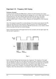
To illustrate this last point, Figure 1 below shows what happens when all but the first two of a 

squarewave’s sinewaves are removed. As you can see, the signal is distorted. 

Figure 1 

16-2 

© 2007 Emona Instruments Experiment 16 – Bandwidth limiting and restoring digital signals

Making matters worse, the channel is like a filter in that it shifts the phase of sinewaves by 

different amounts. Again, to illustrate, Figure 2 below shows the signal in Figure 1 but with one 

of its two sinewaves phase shifted by 40º. 

Figure 2 

Imagine the difficulty a digital receiver circuit such as a PCM decoder would have trying to 

interpret the logic level of a signal like Figure 2. Some, and possibly many, of the codes would 

be misinterpreted and incorrect voltages generated. The makes the recovered message “noisy” 

which is obviously a problem. 

The experiment 

In this experiment you’ll use the Emona DATEx to set up a PCM communications system. Then 

you’ll model bandwidth limiting of the channel by introducing a low-pass filter. You’ll observe 

the effect of bandwidth limiting on the PCM data using a scope. Finally, you’ll use a comparator 

to restore a digital signal and observe its limitations. 

It should take you about 50 minutes to complete this experiment and an additional 20 minutes 

to complete the Eye-Graph addendum. 

Equipment 

Personal computer with appropriate software installed 

NI ELVIS plus connecting leads 

NI Data Acquisition unit such as the USB-6251 (or a 20MHz dual channel oscilloscope) 

Emona DATEx experimental add-in module 

two BNC to 2mm banana-plug leads 

assorted 2mm banana-plug patch leads 

Experiment 16 – Bandwidth limiting and restoring digital signals © 2007 Emona Instruments 16-3

Procedure 

Part A – The effects of bandwidth limiting on PCM decoding 

As mentioned in the preliminary discussion, bandwidth limiting in a channel can distort digital 

signals and upset the operation of the receiver. This part of the experiment demonstrates this 

using a PCM transmission system. 

1. Ensure that the NI ELVIS power switch at the back of the unit is off. 

2. Carefully plug the Emona DATEx experimental add-in module into the NI ELVIS. 

3. Set the Control Mode switch on the DATEx module (top right corner) to PC Control. 

4. Check that the NI Data Acquisition unit is turned off. 

5. Connect the NI ELVIS to the NI Data Acquisition unit (DAQ) and connect that to the 

personal computer (PC). 

6. Turn on the NI ELVIS power switch at the back then turn on its Prototyping Board 

Power switch at the front. 

7. Turn on the PC and let it boot-up. 

8. Once the boot process is complete, turn on the DAQ then look or listen for the 

indication that the PC recognises it. 

9. Launch the NI ELVIS software. 

10. Launch the DATEx soft front-panel (SFP) and check that you have soft control over the 

DATEx board. 

11. Slide the NI ELVIS Function Generator’s Control Mode switch so that it’s no-longer in 

the Manual position. 

12. Launch the Function Generator’s VI. 

13. Press the Function Generator VI’s ON/OFF control to turn it on. 

14. Adjust the Function Generator using its soft controls for an output with the following 

specifications: 

 

 

 

 

Waveshape: Sine 

Frequency: 20Hz 

Amplitude: 4Vp-p 

DC Offset: 0V 

15. Minimise the Function Generator’s VI. 



16. Connect the set-up shown in Figure 3 below. 

MASTER 

SIGNALS 

FUNCTION 

GENERATOR 

PCM 

ENCODER 

PCM 

DECODER 

GND 

PCM 

100kHz 

SINE 

ANALOG I/ O 

TDM 

TDM 

SCOPE 

CH A 

100kHz 

COS 

ACH1 

DAC1 

INPUT 2 

FS 

FS 

CH B 

100kHz 

DIGITAL 

8kHz 

DIGITAL 

2kHz 

DIGITAL 

2kHz 

SINE 

ACH0 DAC0 

VARIABLE DC 

+ 

INPUT 1 

CLK 

PCM 

DATA 

PCM 

DATA 

CLK 

OUTPUT2 

OUTPUT 

TRIGGER 

Figure 3 

This set-up can be represented by the block diagram in Figure 4 below. The PCM Encoder 

module converts the Function Generator’s output to a digital signal which the PCM Decoder 

returns to a sampled version of the original signal. Importantly, the patch lead that connects 

the PCM Encoder module’s PCM DATA output to the PCM Decoder module’s PCM DATA input is 

the communication system’s “channel”. 

Function 

Generator 

Message 

To Ch.A 

"Stolen" FS 

20Hz 

IN 

The channel 

Output 

To Ch.B 

CLK 

"Stolen" CLK 

2kHz 

Master 

Signals 

PCM Encoding 

PCM Decoding 

Figure 4 


17. Launch the NI ELVIS Oscilloscope VI. 

18. Set up the scope per the procedure in Experiment 1 with the following change: 

 

Timebase control to 10ms/div instead of 500µs/div 

19. Activate the scope’s Channel B input to observe the PCM Decoder module’s output as well 

as the PCM Encoder module’s input. 

Note: If the set-up is working, you should see a 20Hz sinewave for the message and its 

sampled equivalent out of the PCM Encoder module. 

Ask the instructor to check 

your work before continuing. 



20. Locate the Tuneable Low-pass Filter module on the DATEX SFP and set its soft Gain 

control to about the middle of its travel. 

21. Turn the Tuneable Low-pass Filter module’s soft Cut-off Frequency Adjust control to 

about the middle of its travel. 

22. Modify the set-up as shown in Figure 5 below. 

MASTER 

SIGNALS 

FUNCTION 

GENERATOR 

PCM 

ENCODER 

TUNEABLE 

LPF 

PCM 

DECODER 

GND 

PCM 

f C x10 0 

100kHz 

SINE 

ANALOG I/ O 

TDM 

TDM 

SCOPE 

CH A 

100kHz 

COS 

100kHz 

DIGITAL 

ACH1 

DAC1 

INPUT 2 

FS 

f C 

FS 

CH B 

8kHz 

DIGITAL 

2kHz 

DIGITAL 

2kHz 

SINE 

ACH0 DAC0 

VARIABLE DC 

+ 

INPUT 1 

CLK 

PCM 

DATA 

GAIN 

PCM 

DATA 

CLK 

OUTPUT2 

OUTPUT 

TRIGGER 

IN 

OUT 

Figure 5 

The set-up can be represented by the block diagram in Figure 6 below. The Tuneable Low-pass 

Filter module models bandwidth limiting of the channel. 

Message 

To Ch.A 

Tuneable LPF 

"Stolen" FS 

20Hz 

IN 

OUTPUT 

To Ch.B 

CLK 

"Stolen" CLK 

2kHz 

Figure 6 


23. Slowly turn the Tuneable Low-pass Filter module’s soft Cut-off Frequency Adjust 

control anti-clockwise. 

Tip: Use the keyboard’s TAB and arrow keys to make fine adjustment of this control. 

24. Stop the moment the PCM Decoder module’s output contains the occasional error. 

Question 1 

What’s causing the errors on the PCM Decoder module’s output? Tip: If you’re not sure, 

see the preliminary discussion. 

Question 2 

If this were a communications system transmitting speech, what would these errors 

sound like when the message is reconstructed? 

25. Reduce the channel’s bandwidth further to observe the effect of severe bandwidth 

limiting of the channel on the PCM Decoder module’s output. 





You have just seen what bandwidth limiting has done to the sampled signal in the time domain 

so now let’s look at what happens in the frequency domain. 

26. Increase the channel’s bandwidth just until the PCM Decoder’s output no-longer contains 

errors. 

27. Suspend the scope VI’s operation by pressing its RUN control once. 

28. Launch the NI ELVIS Dynamic Signal Analyzer VI. 

29. Adjust the Signal Analyzer’s controls as follows: 

General 

Sampling to Run 

Input Settings 

 

Source Channel to Scope CHB 

Voltage Range to ±10V 

FFT Settings 

Frequency Span to 1,000 

Resolution to 400 

Window to 7 Term B-Harris 

Averaging 

Mode to RMS 

Weighting to Exponential 

# of Averages to 3 

Triggering 

 

Triggering to Immediate 

Frequency Display 

 

Units to dB 

 

Markers to OFF (for now) 

 

RMS/Peak to RMS 

 

Scale to Auto 

30. Activate the Signal Analyzer’s markers by pressing the Markers button. 

31. Use the Signal Analyzer’s M1 marker to examine the frequency of the sinewaves that 

make up the sampled message. 

32. Use the M1 marker to locate the sinewave in the sampled message that has the same the 

frequency as the original message. 


33. Reduce the channel’s bandwidth so that the PCM Decoder module’s output contains 

occasional errors and observe the effect on the signal’s spectral composition. 

Tip: Use the Signal Analyzer’s lower display (which is basically a scope) to help you set 

the level of errors. 

34. Reduce the channel’s bandwidth so that the PCM Decoder module’s output is severely 

bandwidth limited and observe the effect on the signal’s spectral composition. 

Question 3 

The Signal Analyzer’s trace should now be much smother than it was before (that is, 

fewer peaks and troughs). What is this telling you about the spectral composition of the 

PCM Decoder module’s output? 

Question 4 

These extra sinewaves are heard as noise. Why doesn’t the Tuneable Low-pass Filter 

module remove them? 





Part B – The effects of bandwidth limiting on a digital signal’s shape 

You’ve seen how a channel’s bandwidth can upset a receiver’s operation. Now let’s have a look at 

how it affects the shape of the digital signal at the receiver’s input. 

Importantly, digital signals that are generated by a message such as a sinewave, speech or 

music cannot be used for this part of the experiment. This is because the data stream is too 

irregular for the scope to be able to lock onto the signal and show a stable sequence of 1s and 

0s. To get around this problem the Sequence Generator module’s 32-bit sequence is used to 

model a digital data signal. 

35. Close the Signal Analyzer VI. 

36. Completely dismantle the previous set-up. 

37. Set the Tuneable Low-pass Filter module’s soft Gain control to about the middle of its 

travel. 

38. Turn the Tuneable Low-pass Filter module’s soft Cut-off Frequency Adjust control fully 

clockwise. 

39. Locate the Sequence Generator module on the DATEx SFP and set its soft dip-switches 

to 00. 

40. Connect the set-up shown in Figure 7 below. 

MASTER 

SIGNALS 

SEQUENCE 

GENERATOR 

TUNEABLE 

LPF 

O 

LINE 

CODE 

100kHz 

SINE 

1 

OO NRZ-L 

SYNC 

O1 Bi-O 

1O RZ-AMI 

11 NRZ-M 

X 

f C x100 

SCOPE 

CH A 

100kHz 

COS 

100kHz 

DIGITAL 

8kHz 

DIGITAL 

2kHz 

DIGITAL 

2kHz 

SINE 

Y 

CLK 

SPEECH 

GND 

GND 

f C 

GAIN 

IN OUT 

CH B 

TRIGGER 

Figure 7 

This set-up can be represented by the block diagram in Figure 8 on the next page. The 

Sequence Generator module is used to model a digital signal and its SYNC output is used to 

trigger the scope to provide a stable display. 


Master 

Signals 

Sequence 

Generator 

Tuneable LPF 

Digital signal 

To Ch.A 

2kHz 

CLK 

Bandwidth limited 

digital signal 

To Ch.B 

SYNC 

SYNC 

To Trig. 

Digital signal modelling 

BW limited channel 

Figure 8 

41. Restart the scope’s VI by pressing its RUN control once. 

42. Adjust the following scope controls: 

 

 

Trigger Source control to TRIGGER instead of CH A 


43. Note the effects of making the channel’s bandwidth narrower by turning the Tuneable 

Low-pass Filter module’s soft Cut-off Frequency Adjust control anti-clockwise. 

Question 5 

What two things are happening to cause the digital signal to change shape? Tip: If 

you’re not sure, see the preliminary discussion. 





An obvious solution to the problem of bandwidth limiting of the channel is to use a transmission 

medium that has a sufficiently wide bandwidth for the digital data. In principle, this is a good 

idea that is used - certain cable designs have better bandwidths than others. However, as 

digital technology spreads, there are demands to push more and more data down existing 

channels. To do so without slowing things down requires that the transmission bit rate be 

increased. This ends up having the same effect as reducing the channel’s bandwidth. The next 

part of the experiment demonstrates this. 

44. Turn the Tuneable Low-pass Filter module’s soft Cut-off Frequency Adjust control fully 

clockwise to make the channel’s bandwidth as wide as possible (about 13kHz). 

45. Launch the Function Generator’s VI. 

46. Adjust the Function Generator for a 2kHz output. 

Note: It’s not necessary to adjust any other controls as the Function Generator’s SYNC 

output will be used and this is a digital signal. 


Note: As you have set up the Function Generator’s output for a signal that’s the same as 

the Master Signals module’s 2kHz DIGITAL output, the signals on the scope shouldn’t 

change. 

FUNCTION 

GENERATOR 

SEQUENCE 

GENERATOR 

TUNEABLE 

LPF 

O 

LINE 

CODE 

ANALOG I/ O 

1 

OO NRZ-L 

SYNC 

O1 Bi-O 

1O RZ-AMI 

11 NRZ-M 

f C x100 

SCOPE 

CH A 

X 

ACH1 

DAC1 

CLK 

Y 

f C 

CH B 

ACH0 DAC0 

VARIABLE DC 

+ 

SPEECH 

GND 

GAIN 

TRIGGER 

GND 

IN 

OUT 

Figure 9 


The set-up in Figure 9 can be represented by the block diagram in Figure 10 below. Notice that 

the Sequence Generator module’s clock is now provided by the Function Generator’s output and 

so it is variable. 

Function 

Generator 

CLK 

Variable 

frequency 

SYNC 


To Ch.A 



To Ch.B 

SYNC 

To Trig. 


BW limited channel 

Figure 10 

48. To model increasing the transmission bit-rate, increase the Function Generator’s output 

frequency in 5,000Hz intervals until the clock is about 50kHz. 

Tip: As you do this, you’ll need to adjust the scope’s Timebase control as well so that you 

can properly see the digital signals. 

Question 6 

What other change to your communication system distorts the digital signal in the same 

way as increasing its bit-rate? 





Part C – Restoring digital signals 

As you have seen, bandwidth limiting distorts digital signals. As you have also seen, digital 

receivers such as PCM decoders have problems trying to interpret bandwidth limited digital 

signals. The trouble is, bandwidth limiting is almost inevitable and its effects get worse as the 

digital signal’s bit-rate increases. 

To manage this problem, the received digital signal must be cleaned-up or “restored” before it 

is decoded. A device that is ideal for this purpose is the comparator. Recall that the 

comparator amplifies the difference between the voltages on its two inputs by an extremely 

large amount. This always produces a heavily clipped or “squared-up” version of any AC signal 

connected to one input if it swings above and below a DC voltage on the other input. 

As you know, ordinarily we avoid clipping but in this case it’s very useful. The bandwidth limited 

digital signal is connected to one of the comparator’s inputs and a variable DC voltage is 

connected to the other. The bandwidth limited digital signal swings above and below the DC 

voltage to produce a digital signal on the comparator’s output. Then, the variable DC voltage is 

adjusted until this happens at the right points in the bandwidth limited digital signal for the 

comparator’s output to be a copy of the original digital signal. 

Unfortunately, this simple yet clever idea has its limitations. First, bandwidth limiting can 

distort the digital signal too much for the comparator to restore accurately (that is, without 

errors). Second, the channel can cause the received digital signal (and the hence the restored 

digital signal) to become phase shifted. For reasons not explained here this can cause other 

problems for receivers. 

This part of the experiment lets you restore a bandwidth limited digital signal using a 

comparator and observe these limitations. 

49. Slide the NI ELVIS Variable Power Supplies’ positive output Control Mode switch so that 

it’s no-longer in the Manual position. 

50. Launch the Variable Power Supplies VI. 

51. Set the Variable Power Supplies’ positive output to 0V by pressing its RESET button. 

52. Set the scope’s Timebase control to the 1ms/div position. 


53. Disconnect the patch lead to the Function Generator’s output then modify the set-up as 

shown in Figure 11 below. 

MASTER 

SIGNALS 

SEQUENCE 

GENERATOR 

O 

LINE 

CODE 

TUNEABLE 

LPF 

FUNCTION 

GENERATOR 

UTILITIES 

COM PARATOR 

REF 

100kHz 

SINE 

100kHz 

COS 

100kHz 

DIGITAL 

8kHz 

DIGITAL 

2kHz 

DIGITAL 

2kHz 

SINE 

1 

OO NRZ-L 

O1 Bi-O 

1O RZ-AMI 

11 NRZ-M 

CLK 

SPEECH 

GND 

GND 

X 

Y 

SYNC 

IN 

f C 

GAIN 

f C x10 0 

OUT 

ANALOG I/ O 

ACH1 

ACH0 

VARIABLE DC 

+ 

DAC1 

DAC0 

IN OUT 

RECTIFIER 

DIODE & RC LPF 

RC LPF 

SCOPE 

CH A 

CH B 

TRIGGER 

Figure 11 

The entire set-up can be represented by the block diagram in Figure 12 below. The comparator 

on the Utilities module is used to restore the bandwidth limited digital signal. 


modelling 

BW limited 

channel 

Restoration 

2kHz 

CLK 

SYNC 

REF 

IN 

Restored 


To Ch.B 


To Ch.A 

SYNC 

To Trig. 

Figure 12 

16-16 


54. Compare the signals. 

Question 7 

Although the restored digital signal is almost identical to the original digital signal, 

there is a difference. Can you see what it is? Tip: If you can’t, set the scope’s Timebase 

control to the 100µs/div position. 

Question 8 

Can this difference be ignored? Why? 



55. Return the scope’s Timebase control to the 1ms/div position. 

56. Increase the Variable Power Supplies’ positive output in 0.2V intervals and observe the 

effect. 

Question 9 

Why do some DC voltages cause the comparator to output the wrong information? Tip: 

If you’re not sure, see the notes on page 16-17. 




1ORZ-AMI 

57. Return the Variable Power Supplies positive output to 0V. 

58. Slowly make the channel’s bandwidth narrower by turning the Tuneable Low-pass Filter 

module’s soft Cut-off Frequency Adjust control anti-clockwise. 

Note: As you do this, the phase difference between the two digital signals will increase 

but ignore this. 

Question 10 

Why does the comparator begin to output the wrong information when this control is 

turned far enough? 

59. Make the channel’s bandwidth wider and stop when the comparator’s output is the same 

as the original digital signal (ignoring the phase shift). 

60. Compare the restored digital signal with the bandwidth limited digital signal by 

modifying the set-up as shown in Figure 13 below. 

MASTER 

SIGNALS 

SEQUENCE 

GENERATOR 

O 

LINE 

CODE 

TUNEABLE 

LPF 

FUNCTION 

GENERATOR 

UTILITIES 

COM PARATOR 

REF 

10kHz 

SINE 

10kHz 

COS 

10kHz 

DIGITAL 

8kHz 

DIGITAL 

2kHz 

DIGITAL 

2kHz 

SINE 

ONRZ-L 

O1Bi-O 

1NRZ-M 

1 

SYNC 

X 

Y 

CLK 

SPECH 

GND 

f C 

GAIN 

f C x10 0 

ANALOG I/ O 

ACH1 DAC1 

ACH0 DAC0 

VARIABLE DC 

+ 

IN OUT 

RECTIFIER 

DIODE & RC LPF 

RC LPF 

SCOPE 

CHA 

CHB 

TRIGER 

GND 

IN 

OUT 

Figure 13 



Question 11 

How can the comparator restore the bandwidth limited digital signal when it is so 

distorted? 


your work before finishing. 


Eye diagrams 

Regardless of whether the digital data is received from a satellite or the optical head 

of a CD drive, it’s important to be able to inspect and test its distortion (that is, the 

channel bandwidth & phase characteristics) and degradation (that is, the channel 

noise). One method of doing so involves using the received digital signal to develop an 

Eye Diagram. 

Eye diagrams can be readily set-up using a stand-alone scope or an Eye Diagram Virtual 

Instrument if the NI ELVIS test equipment is being used. For both, multiple sweeps of 

the scope are overlayed one upon another producing a display much like Figure 1 below. 

Figure 1 

As you can see, the spaces between the logic-1s and logic-0s produce “eyes” in the 

centre of the display. Importantly, the greater the effect of bandwidth limiting and 

phase distortion, the less ideal the logic levels become and so the eyes begin to “close”. 

In addition, channel noise appears as erratic traces across the centre of the eye 

though a scope with a very long persistence is needed to capture them if the Eye 

Diagram VI is not being used. 

If time permits, this activity gets you to develop an Eye Diagram and observe the 

effect of noise and bandwidth limiting on its eyes. 



1. Completely dismantle the existing set-up. 

Note: If you’re attempting this part of the experiment without having just completed 

the previous part, perform Steps 1 to 10 on page 16-4. 

2. Check that the Sequence Generator module’s soft dip-switches are set to 00. 

3. Connect the set-up shown in Figure 2 below. 

NOISE 

GENERATOR 

FUNCTION 

GENERATOR 

SEQUENCE 

GENERATOR 

CHANNEL 

MODULE 

0dB 

O 

LINE 

CODE 

-6 dB 

-20dB 

AMPLIFIER 

ANALOG I/ O 

ACH1 

DAC1 

1 

OO NRZ-L 

O1 Bi-O 

1O RZ-AMI 

11 NRZ-M 

CLK 

X 

Y 

SYNC 

CHANNEL 

BPF 

BASEBAND 

LPF 

ADDER 

SCOPE 

CH A 

CH B 

IN 

GAIN 

OUT 

ACH0 DAC0 

VARIABLE DC 

+ 

SPEECH 

GND 

NOISE 

SIGNAL 

CHANNEL 

OUT 

TRIGGER 

GND 

Figure 2 

This set-up can be represented by the block diagram in Figure 3 below. 

Function 

Generator 

Sequence 

Generator 

Adder 

Baseband 

LPF 

CLK 


noisy digital signal 

Bit-clock 

To Ch.B & Trig 

Noise 

generator 

Noisy digital 

signal 

To Ch.A 


Noisy & bandwidth limited channel 

Figure 3 


The Sequence Generator module is used to model a digital signal and its bit-clock is provided 

by the function generator so the data rate can be varied. An Adder is used to add noise to the 

digital signal that can be varied from -20dB (lowest) to 0dB (highest. The signal is finally 

bandwidth limited by the Baseband LPF. 

4. Slide the NI ELVIS Function Generator’s Control Mode switch so that it’s in the Manual 

position. 

5. Launch the NI ELVIS Oscilloscope VI. 

6. Set up the scope per the procedure in Experiment 1 with the following changes: 

 

 

Trigger Source control to TRIGGER instead of CH A 


7. Activate the scope’s Channel B input to observe the Sequence Generator module’s bitclock 

as well as the digital data on the Tuneable Low-pass Filter module’s output. 

8. Use the Function Generator’s hard frequency adjust controls to set the Sequence 

Generator module’s bit-clock frequency to 2kHz (as measured using the scope). 

Note: Once done, you should observe a digital signal with an obvious noise component. 

9. Increase the digital signal’s noise component to -6dB and observe the effect. 

10. Increase the digital signal’s noise component to 0dB and observe the effect. 

11. Return the digital signal’s noise component to -20dB. 


NOISE 

GENERATOR 

FUNCTION 

GENERATOR 

SEQUENCE 

GENERATOR 

CHANNEL 

MODULE 

LINE 

CODE 

0dB 

O 

-6 dB 

-20dB 

AMPLIFIER 

ANALOG I/ O 

ACH1 

DAC1 

1 

OO NRZ-L 

O1 Bi-O 

1O RZ-AMI 

11 NRZ-M 

CLK 

X 

Y 

SYNC 

CHANNEL 

BPF 

BASEBAND 

LPF 

ADDER 

SCOPE 

CH A 

CH B 

IN 

GAIN 

OUT 

ACH0 DAC0 

VARIABLE DC 

+ 

SPEECH 

GND 

NOISE 

SIGNAL 

CHANNEL 

OUT 

TRIGGER 

GND 

Figure 4 



This set-up can be represented by the block diagram in Figure 5 below. 

Function 

Generator 

Sequence 

Generator 

Adder 

Baseband 

LPF 

CLK 


noisy digital signal 

To Ch.A 

Bit-clock 

To Ch.B & Trig 

Noise 

generator 


Noisy & bandwidth limited channel 

Figure 5 

13. Repeat Steps 9 and 10 and observe the effect on the digital signal. 

Question 1 

Why has the noise disappeared? 

Note: Although much of the noise has been removed, this doesn’t mean that the digital signal 

is now unaffected. The remaining noise can still distort the digital signal enough to cause 

errors at the receiver. You can see the errors for yourself if you compare the signals with - 

20dB and 0dB of noise. 




14. Set the digital signal’s noise component to -6dB. 

15. Close all NI ELVIS VIs. 

16. Close the NI ELVIS software. 

17. Launch the DATEx Eye-Graph virtual instrument per the instructor’s directions. 

18. Once the Eye-Graph VI has initialised, activate it by pressing the RUN button on the 

VI’s toolbar. 

Note: Once done, multiple traces of a scope’s sweep for Channel A (the noisy bandwidth 

limited digital signal) are written on the Eye-Graph VI’s screen. This will produce an eye 

diagram similar to the one shown in Figure 1. 



19. Stop the DATEx Eye-Graph VI by pressing its STOP button. 

20. Increase digital signal’s noise component to 0dB. 

21. Run the Eye-Graph VI again and watch it for a couple of minutes to observe the effect. 

Question 2 

What’s the relationship between the size of the eye and the level of noise that the 

channel introduces to digital signal? 





22. Stop the DATEx Eye-Graph VI. 

23. Increase the digital signal’s data rate by increasing the Sequence Generator module’s 

bit-clock. 

Note 1: To do this, turn the Function Generator’s FINE FREQUENCY control about one 

quarter of a turn. 

Note 2: By increasing the digital signal’s data rate, you’ll increase the effect of 

bandwidth limiting. 

24. Run the Eye-Graph VI again and watch it for a couple of minutes to observe the effect. 

Question 3 

What’s the relationship between the size of the eye and the distortion level of the 

received digital signal? 


your work before finishing.

Experiment 16 â Bandwidth limiting and restoring digital signals

You also want an ePaper? Increase the reach of your titles

Delete template?

Save as template?

Experiment 16 â Bandwidth limiting and restoring digital signals