Master Thesis Stefan Jansen, Niels Bohr Institute, University of ...

PARAMETER INVESTIGATION FOR 

SUBSURFACE TOMOGRAPHY WITH 

REFRACTION SEISMIC DATA 

Master Thesis in Geophysics 

STEFAN JANSEN 

Niels Bohr Institute, University of Copenhagen 

Supervisors: 

Klaus Mosegaard, University of Copenhagen 

Roger Wisén, Rambøll Danmark 

2 nd November 2010

Master Thesis in Geophysics 

Title: Parameter Investigation for Subsurface Tomography with Refraction 

Seismic Data 

Author: Stefan Jansen 

CPR no.: 201170 

E-mail: stefan.jansen@vip.cybercity.dk 

ECTS points: 60 

Supervisor: Klaus Mosegaard, University of Copenhagen 

External Supervisor: Roger Wisén, Rambøll Danmark 

Submitted: 2 nd November 2010 

Updated: 5 th January 2011

Abstract 

For planned highway and railway improvements in Norway tomographic i- 

mages were modelled supplementary to results obtained from a layer based interpretation 

tool like for example the Generalized Reciprocal Method (GRM). 

In general good agreements between these methods were achieved, but some 

inconsistencies led to questions whether the tomographic inversions can be 

improved. 

In this master thesis the tomographic inversion tool Rayfract has been examined 

thoroughly with the aim of determining settings and parameters leading 

to tomographic images with increased velocity contrast. 

With the help of synthetic models containing various kinds of anomalies the 

sensitivity of the tool has been investigated. A thorough parameter investigation 

on one of these models led to the determination of six combinations of 

settings and parameters for obtaining an improved absolute RMS-error and 

model resemblance. Verification of these combinations with a model resembling 

one of the profiles from Norway showed unexpected responses. Finally 

these findings were applied to field data. 

Over all this work shows that two parameters, Smoothing and wavepath 

width, are decisive for the quality of all conducted inversions. These parameters 

are both directly or indirectly linked to smoothing of the result. Even 

if a fixed recipe for the choice of parameters can not be given, as they are 

dependent on the topography and subsurface condition of each individual 

profile, this thesis clearly defines the parameters in focus and how to perform 

a quick and reliable parameter test for each new situation. 

i

Contents 

Contents 

iii 

1 Introduction 1 

2 Refraction Seismology 5 

2.1 CMP-Refraction Seismology . . . . . . . . . . . . . . . . . . . 10 

3 The Generalized Reciprocal Method (GRM) 13 

4 Rayfract® Seismic Refraction & Borehole Tomography 17 

4.1 Delta-t-V Inversion . . . . . . . . . . . . . . . . . . . . . . . . 18 

4.1.1 Traveltime Field Computation . . . . . . . . . . . . . . 20 

4.2 Smooth Inversion . . . . . . . . . . . . . . . . . . . . . . . . . 23 

4.3 WET Wavepath Eikonal Traveltime tomography . . . . . . . . 24 

4.3.1 Fresnel volume - Fat Rays . . . . . . . . . . . . . . . . 27 

5 Investigations 29 

5.1 Sensitivity Investigation . . . . . . . . . . . . . . . . . . . . . 29 

5.1.1 Synthetic Models . . . . . . . . . . . . . . . . . . . . . 32 

5.1.2 Results of Sensitivity Investigation . . . . . . . . . . . 33 

5.2 Parameter Investigation . . . . . . . . . . . . . . . . . . . . . 35 

5.2.1 Smooth Inversion Settings . . . . . . . . . . . . . . . . 37 

5.2.2 Delta-t-V Inversion Settings and Parameters . . . . . . 38 

5.2.3 WET Tomography Inversion Settings and Parameters . 42 

6 Results of the Parameter Investigations 45 

6.1 Smooth Inversion . . . . . . . . . . . . . . . . . . . . . . . . . 45 

6.1.1 Smooth Inversion Settings . . . . . . . . . . . . . . . . 45 

6.1.2 Delta-t-V Inversion . . . . . . . . . . . . . . . . . . . . 48 

6.2 WET Tomo . . . . . . . . . . . . . . . . . . . . . . . . . . . . 50 

6.2.1 General WET Tomo Settings . . . . . . . . . . . . . . 50 

iii

6.2.2 Interactive WET Tomo Parameters . . . . . . . . . . . 51 

6.3 Combined Settings . . . . . . . . . . . . . . . . . . . . . . . . 54 

7 Case Ørbekk 59 

8 Ørbekk Field Data Processing 65 

8.1 Default Settings and Parameters . . . . . . . . . . . . . . . . . 65 

8.2 Combinations of Best Settings and Parameters . . . . . . . . . 68 

9 Sources of Uncertainties 71 

10 Conclusion and Prospects 73 

A Eikonal solver by Vidale 77 

B Refractor-imaging principle 79 

C Sensitivity Investigation 81 

C.1 Synthetic Models . . . . . . . . . . . . . . . . . . . . . . . . . 81 

C.1.1 Synthetic models with faults . . . . . . . . . . . . . . . 92 

D Results of the Parameter Investigation 99 

D.1 Tomogram of the Reference Model . . . . . . . . . . . . . . . 99 

D.2 Smooth Inversion . . . . . . . . . . . . . . . . . . . . . . . . . 100 

D.2.1 Smooth Inversion Settings . . . . . . . . . . . . . . . . 100 

D.2.2 Delta-t-V Inversion Settings . . . . . . . . . . . . . . . 101 

D.2.3 Parameters for Interactive Delta-t-V Inversion . . . . . 103 

D.3 WET Tomography . . . . . . . . . . . . . . . . . . . . . . . . 104 

D.3.1 WET Tomography Settings . . . . . . . . . . . . . . . 104 

D.3.2 Settings for Forward modelling . . . . . . . . . . . . . 106 

D.3.3 Interactive WET Tomomography Parameters . . . . . 107 

D.4 Combinations of Settings and Parameters . . . . . . . . . . . . 109 

D.4.1 Tomograms after 50 iterations . . . . . . . . . . . . . . 111 

D.4.2 Tomograms after 250 iterations . . . . . . . . . . . . . 112 

E Case Ørbekk - Inversion Results 113 

F Additional Analysis 117 

G Further Improvements 119 

Bibliography 121 

iv

Chapter 1 

Introduction 

Seismic tomography, also known as Refraction tomography, has in recent 

years gained increasing interest in near-surface processing. This method is 

able to overcome the constraints faced by conventional methods (Sheehan 

et al., 2005). Therefore it has become an interesting method for geotechnical 

applications where the near subsurface is explored. 

As many other geophysical methods, the refraction seismology has the aim 

of surveying the structure and physical properties of the subsurface from 

measurements taken on the surface. The refraction seismology is capable 

of determining the velocity of the layer beneath the weathering layer (top 

layer), called the refractor; this can not be achieved with reflection seismology. 

Refraction seismology is used for determining wave-velocities and layer 

thicknesses of the weathering layers, and for surveys for mapping larger a- 

reas and velocity determination of unknown areas as well as various other 

applications (Gebrande and Miller, 1985). Data processing is handled by the 

use of CMP (Common Mid-Point) refraction seismology, which simplifies the 

arrangement of sources and receivers as in reflection seismology. 

Conventional processing tools/interpretation methods, as for example delaytime 

and Plus-Minus-method or GRM (Generalized Reciprocal Method) analysis, 

make simplifying assumptions about the velocity structure that conflict 

with frequently observed near-surface attributes such as heterogeneity, lateral 

discontinuities, and gradients (Sheehan et al., 2005). Refraction tomography 

is not subject to these constraints and is therefore able to resolve velocity gradients 

and lateral velocity changes and can be applied in geological conditions

2 Introduction 

where conventional refraction techniques fail, such as areas of compaction, 

karst, and fault zones (Zhang and Toksoz, 1998). 

Tomographic imaging has been conducted by Rambøll Danmark with the 

tomographic code Rayfract ® by Intelligent Resources Inc., which inversions 

are based on Wavepath Eikonal Traveltime (WET) (Schuster and Quintus- 

Bosz, 1993), and directly compared to the layer based interpretation method 

Generalized Reciprocal Method (GRM). As the results of these different methods 

did not correlate perfectly the questions 

- Has the program been used correctly with respect to settings and chosen 

parameters? 

- Is it possible to improve the quality/velocity contrast of the tomograms? 

have been raised. 

In this thesis the functions of the program Rayfract ® , which creates 2D 

tomograms from refraction seismic data, are investigated in order to find the 

optimal settings and parameters for obtaining tomographic images with the 

best possible velocity contrast. 

Before the parameter investigation the code’s ability to recognize different 

objects in the subsurface is examined. Synthetic models with vertical anticlines 

and synclines (holes in the refractor) of different widths, anomalies 

- shaped as squares 

- with the shape of rectangulars 

- in different dimensions 

- with different velocities 

- in various locations 

as well as faults 

- with different sloping angles

3 

- with different widths 

are created for computing first arrival traveltimes. Also part of this investigation 

is the inspection of the difference between high and sparse shot and 

receiver coverage. From these models the best suited model for the subsequent 

parameter investigations is chosen as the reference model with default 

code settings. 

The parameter investigation is carried out by changing only one parameter at 

a time in order to see the influence of each parameter and setting individually. 

As a comparison criterion the resulting absolute RMS-error and normalized 

RMS-error, computed as the RMS-error divided by maximum pick time of 

all traces modelled, are good choices. 

After having studied the influence of all relevant settings and parameters, 

the ones giving the best results with respect to RMS-error are collected in 

different combinations. As a result of this study it is expected to find a 

combination, which yields a tomographic inversion with a better velocity 

contrast compared to the default settings and parameters. 

The thus determined settings and parameters are then applied to traveltimes, 

which are computed from a model resembling an extract of a real profile; this 

includes the station and shot coordinates from the original measurements. 

Finally with the combination, which yields the best result, a tomographic 

model from real measurement data is created. As the aim of this work is to 

improve the contrast of earlier obtained images the same field data are used. 

This way the direct comparison of the results reveals the dimension of the 

improvement. 

In chapter 2 the theory of refraction and CMP-Refraction seismology is discussed. 

Then a short description of the layer based interpolation tool Generalized 

Reciprocal Method (GRM) in chapter 3 is followed by an elaboration 

of the inversion processes the Rayfract code is built on (chapter 4). The 

actual parameter investigation follows the description of the examined sensitivity 

models and their outcome in chapter 5. After the investigation with 

synthetic data is completed the gained knowledge is applied to real survey 

data as described in chapter 8. The report rounds up with the discussion 

of possible uncertainties in chapter 9 and the conclusions and prospects in 

chapter 10.

4 Introduction 

In the Appendix all synthetic models and their respective tomograms as 

well as all parameter investigation results and the combined solutions can be 

found. 

For reading this report it is necessary to read it in parallel with the Appendix. 

A large number of investigations generated a tremendous amount of data and 

images and presenting them in the Appendix provides a more fluent read. 

However, tomographic images with the desired positive effect are integrated 

in the text and discussed there.

Chapter 2 

Refraction Seismology 

In order to determine the velocity structure of the subsurface the refraction 

seismology is a very important tool. This chapter provides a short review of 

the theory behind refraction seismology. 

A seismic ray that strikes the boundary of two layers, which mark the change 

in seismic velocity, is partitioned into a reflected and refracted ray. The angles 

the reflected and refracted waves form with the vertical plane are described 

by the law of reflection and law of refraction. The latter one is also known as 

Snell’s law (equation 2.0.1) with angles and velocities as illustrated in figure 

2.1. 

sin(i) 

v 1 

= sin(β) 

v 2 

= s (2.0.1) 

Incoming ray 

Reflected ray 

i 

i 

υ1 

β 

υ2 

Refracted ray 

Figure 2.1: An incoming ray strikes the boundary of two media with different velocities (v 2 

> v 1 ) and is partitioned into a reflected and refracted ray.

6 Refraction Seismology 

The quantity s is the horizontal slowness, also called the raypath parameter, 

and has the same value for incident, reflected and refracted waves. 

The incoming and reflected ray experience the same layer properties, hence 

their angles to the vertical plane are equal. For velocity v 2 greater than v 1 

the angle β becomes larger than angle i and vice versa. When β assumes the 

angle 90 degrees the refracted ray travels horizontally in the lower medium, 

parallel to the interface between the two media. This wave is also referred to 

as the headwave and it has the unique property that it continually transmits 

energy back into the upper layer as it travels along the interface (Lay and 

Wallace, 1995). The angle of incidence that causes this phenomenon is called 

the critical angle, i c and is defined as: 

i c = arcsin(v 1 /v 2 ). (2.0.2) 

For the case where the angle i is greater than i c it is impossible to satisfy 

Snell’s law as sin(β) cannot reach unity (Telford et al., 2004). No refracted 

ray exist and all energy is reflected back into the upper layer (total reflection). 

If v 2 is smaller than v 1 no critical angle exists and the refracted ray is 

deflected toward vertical. 

Traveltimes: 

For the determination of the velocities of the subsurface layers the traveltime 

is a very important parameter. The traveltime as a function of distance 

provides a direct measure of velocity at depth. As mentioned above, the 

reflected and refracted waves are the resulting travel paths when the lower 

velocity, v 2 , is greater than the upper velocity, v 1 . Furthermore, there is 

the direct arrival, which travels in a straight line between the source (i.e. an 

explosion) and receiver (i.e. a geophone or hydrophone). In figure 2.2 the 

explosion is marked as an asterisk, the receiver as ∇ and the distance the 

direct wave travels between them as ∆.

7 

★ 

Δ 

▽ 

direct 

H 

ic 

i 

i 

reflected 

ic 

υ 1 

refracted 

r 

υ 2 

Figure 2.2: Three principle rays in a layer over a refractor. A headwave is equivalent to the 

distance marked ’r’. 

For the paths shown in figure 2.2 the following three traveltimes for sources 

at the surface and the layer thickness H are found: 

ˆ Traveltime for direct arrival: 

t dir = ∆/v 1 (2.0.3) 

ˆ Traveltime for the reflected arrival: 

t refl = 2H/(cos(i)v 1 ) (2.0.4) 

ˆ Traveltime for the refracted arrival: 

t refr = r/v 2 + 2H/(cos(i c )v 1 ) (2.0.5) 

Here the parameter r is the distance the refracted wave travels in the refractor 

parallel to the intersection. As seen in figure 2.2, the refracted wave 

has travelled a certain horizontal distance in the upper medium before it is 

refracted and turns into a headwave. This implies that at a certain distance 

from the source there cannot be any refracted ray. This distance is also 

referred to as the critical distance, ∆ c , and is defined as: 

∆ c = 2H tan(i c ). (2.0.6)


Substituting the expression for i c in equation (2.0.2) and applying some basic 

trigonometric rules yields the following relation for the critical distance: 

∆ c = 2H tan(arcsin(v 1 /v 2 )) = 

2H 

√ 

. (2.0.7) 

(v 2 /v 1 ) 2 − 1 

For receivers with increasing distance from the source the term r/v 2 in equation 

(2.0.5) becomes more dominant; the wavefront travels along the surface 

with the apparent velocity v 2 . With r = ∆ − 2H tan(i c ) and sin(i c ) = v 1 /v 2 

equation (2.0.5) becomes 

t refr = 

2H 1 

+ 1 ( 

∆ − 2Hv ) 

1 

cos(i c ) v 1 v 2 cos(i c )v 2 

= 2H 

cos(i c ) 

( 1 

+ v ) 

1 

+ ∆ (2.0.8) 

v 1 v 2 

v 2 2 

This is a very useful equation because it separates the travelpath into a 

horizontal and a vertical term (Lay and Wallace, 1995). 

Figure 2.3 shows the traveltime curves for the three primary waves. At 

short distances only the direct (red) and reflected (green) arrivals exist. The 

reflected-arrival traveltime is described by a hyperbola. The intercept time 

τ 1 at ∆=0 has a traveltime of 2H/v 1 . At large distance the reflection traveltime 

becomes asymptotic to the direct arrival. The headwave appears as 

a reflection at the critical distance, ∆ c (Lay and Wallace, 1995). 

1 Intercept time is the traveltime at zero off-set. The time distance curve of the refracted 

line is back-projected to the zero off-set point, where the intercept-time is found. It is not 

a physical meaningful value as no refraction traveltimes exist for offsets less than ∆ c , but 

it is a very useful method for computing the layer thickness. See Telford et al. (2004) for 

details.

9 

slope = 1/υ1 

direct wave 

reflected wave 

refracted wave 

slope = 1/υ2 

τ 

Δc 

Distance Δ 

Figure 2.3: Time-distance curve of the direct, reflected and refracted arrivals. 

Figure 2.4 gives an example of a seismic profile recording of an area in the 

USA. Traveltimes for the direct arrivals, reflected arrivals and refracted arrivals 

are clearly visible and indicated in conformance with the lines in figure 

2.3. 

refracted wave 

direct wave 

reflected wave 

Figure 2.4: Seismic profile recording from Lenox, Tennessee, USA illustrating the three primary 

arrivals at the receivers. Source is a 4 kg sledgehammer, receiver-spacing 1.5 m. Coloured lines 

correspond to lines in figure 2.3. The traveltimes for the refracted wave appear earlier than 

can be seen in this seismogram. Source: http://pubs.usgs.gov/of/2003/ofr-03-218/ 

ofr-03-218.html


2.1 CMP-Refraction Seismology 

The common-midpoint-technique (CMP-technique) is originally known from 

reflection-seismology where it contributed a lot to its progress. Today it is 

almost exclusively used. 

A mid-point is defined as the mid-point between source and receiver position 

and traces are gathered with a common midpoint position. By this all 

reflections, measured at different offsets, are gathered in the same CMPs, 

which contain information of the same subsurface points below the midpoint 

positions. One important reason for this technique is its usage for the subsequent 

stacking where the generally poor signal-to-noise ratio is improved. For 

details about the CMP technique with reflection-seismology refer to Telford 

et al. (2004) or Drijkoningen and Verschuur (2003). 

Gebrande (1986) assumes that the advantages of this technique within reflection-seismology 

can lead to the same simplifications in refraction seismology. 

He derives formulas for the N-layer as well as 2-layer problem. In this thesis 

only the 2-layer-case shall be treated because this case often occurs in reality 

and forms the basis of the several layers problem. 

Figure 2.5 shows a CMP in refraction seismology, where it is defined as the 

midpoint X between the two shotpoints F (forward shot with receiver R) 

and R (reverse shot with receiver F ). 

F 

Δ/2 

X 

Δ/2 

R 

X 

X 

β 

α 

H(B) 

H(X) 

H(A) 

υ 1 

● 

● 

υ 2 

● 

φ 

Figure 2.5: Principle of the CMP Refraction Traveltimes. 

For two layers the CMP-model is described by the layer thickness, H(X), 

measured perpendicular to the layer boundary beneath the CMP X, the 

dipping angle ϕ and the layer velocities v 1 and v 2 .

CMP-Refraction Seismology 11 

Gebrande derives the following equation for the traveltime: 

√ 

t(X, ∆) = 2H(X) ( ) 2 v1 

1 − + ∆ cos(ϕ) . (2.1.1) 

v 1 v 2 v 2 

With this equation the CMP-traveltime can be seen as a function of two 

independent variables, the CMP-coordinates X and the offsets ∆. Partial 

differentiation with ∆ for constant X delivers the reciproke CMP-apparent 

velocity: 

( ) ∂t(X, ∆) 

∂∆ 

X 

= cos(ϕ) 

v 2 

= 1 

V CMP 

. (2.1.2) 

Partial differentiation with X for constant offset ∆ leads to the dipping function: 

( ) ∂t(X, ∆) 

∂X 

∆ 

√ 

= − 2 sin(ϕ) ( ) 2 v1 

1 − . (2.1.3) 

v 1 v 2 

When the velocity of the uppermost layer, v 1 , is known, then the dipping 

angle, ϕ, and refractor velocity, v 2 , or critical angle, i c = arcsin(v 1 /v 2 ), 

respectively, and with the CMP-intercept time, τ, which is the first term 

of equation (2.1.1), the local layer-thickness, H(X), can be determined. 

H(X) = τv 1 

2 

√ 

1 − 

( 

v1 

v 2 

) 2 

−1 

= τv 1 

2 cos(i c ) . (2.1.4) 

In principle this technique is similar to a forward and reverse-shot analysis 

with the advantage that extrapolations to the shotpoints are not necessary, 

but local, at CMP valid layer thicknesses, are found. The refractor is obtained 

as an envelope of circles with radius H(X) around the CMPs at the surface 

(Gebrande, 1986).

12 Refraction Seismology

Chapter 3 

The Generalized Reciprocal 

Method (GRM) 

Earlier made tomographic inversions have been compared to interpretations 

of the refraction seismic processing algorithm Generalized Reciprocal Method 

(GRM). 

The advantage of the GRM inversion algorithms, compared to conventional 

methods, is their emphasis of the lateral resolution of individual layers (Palmer, 

2009). Two inversion algorithms are employed: the refractor velocity analysis 

function t V and the time model algorithm t X . From the refractor velocity 

analysis function (equation (3.0.1)) the refractor velocity is obtained, 

and the time model algorithm ( equation (3.0.2)), also called the generalized 

time-depth, is a measure of the depth of the refractor. Figure 3.1 illustrates 

both algorithms. 

t V = 1 2 (t ∆F − t ∆R + t F R ) (3.0.1) 

t X = 1 2 

( 

( 

t ∆F + t ∆R − t F R + ∆ )) 

F ∆ R 

. (3.0.2) 

V n 

Here t ∆F is the traveltime at receiver ∆ F from forward shot point F , t ∆R 

is the traveltime at receiver ∆ R from reverse shot point R and t F R is the 

reciprocal time between the two shot points. V n is the apparent velocity and

14 The Generalized Reciprocal Method (GRM) 

its value is determined from the velocity analysis as explained below. 

Figure 3.1 clearly illustrates the parts of the traveltimes adding up in these 

equations as solid lines and the parts cancelling out as dashed lines. Figure 

3.1a sketches the reduction in equation (3.0.1) to the approximate traveltime 

from shot point F to a point in the refractor below the CMP X. 

F ΔR X ΔF R 

Vi 

ZX 

tΔR 

tΔF 

tFR 

● 

P 

Q 

Vn 

(a) 

F ΔR X ΔF R 

Vi 

tΔF 

ZX 

tΔR 

tFR 

P 

Q 

Vn 

(b) 

ΔFΔR/Vn 

Figure 3.1: GRM inversion algorithms (a) GRM refractor velocity analysis algorithm (equation 

(3.0.1)) and (b) GRM time model algorithm (generalized time-depth, equation (3.0.2)). 

The most important aspect of the GRM method is the determination of the 

optimum values for the distance ∆ F ∆ R . Optimum ∆ F ∆ R values are found 

where forward and reverse rays emerge from nearly the same point on the 

refractor. Two approaches for the determination of ∆ F ∆ R are Direction 

calculation of ∆ F ∆ R values and Observation of ∆ F ∆ R values, but Palmer 

(1981) does not quote these methods as reliable as the inspection of the velocity 

analysis and time-depth functions, which use a range of ∆ F ∆ R values.

15 

Applying refractor velocity analysis finds the optimum ∆ F ∆ R value by evaluating 

equation (3.0.1) for a range of ∆ F ∆ R -separations between points F 

and R with reference point X midway between F and R. Here the paths 

X∆ R and X∆ F are equal. Plotting t V against distance for several ∆ F ∆ R 

values and fit the obtained t V values for each ∆ F ∆ R value leads to the optimum 

∆ F ∆ R value, where the calculated points have the smallest deviations 

from the fitted line. Deviations can be both positive and negative which 

corresponds to the fact that the optimum ∆ F ∆ R represents an average value 

(Palmer, 1981). The ∆ F ∆ R value zero corresponds to the conventional reciprocal 

method and is similar to the plus term in the Plus-Minus method by 

Hagedoorn (1959), which is shortly described in Appendix B. 

The fitted line for the optimum ∆ F ∆ R has a slope defining the inverse of 

an apparent refractor velocity, V refractor : 

dt V 

d∆ = 1 

= 1 . (3.0.3) 

V refractor V n 

In case of major structures in the subsurface, which can be seen by larger deviations 

from the fitted line, Palmer (1981) developed the following approach 

for determining the optimum ∆ F ∆ R value(s) on either side of the structure. 

A value for major deviation is defined and from the fitted line the first and 

last major deviations are found. Positive and negative deviations are connected 

respectively and their resulting lines intersect on the optimum ∆ F ∆ R 

value. The found value is most likely not the same as the one found at first. 

This results in several optimum ∆ F ∆ R values, one found in the first stage 

and at least one in the second stage. Each value has its unique advantage 

with respect to the subsequent processing and interpretation. 

The time model algorithm t X (eq. (3.0.2)) provides a measure of the depth 

to the refracting interface in units of time (Palmer, 2009). Figure 3.1b illustrates 

the respective ray-paths where the dashed lines cancel each other out 

and the solid lines remain. The term ∆ F ∆ R /V n represents the additional 

traveltime in the refractor between the stations ∆ R and ∆ F . It can be seen 

that the GRM time model is the average of the reverse delay time at ∆ R 

and the forward delay time at ∆ F . Values of optimum ∆ F ∆ R are found by 

calculating time-depths for a range of ∆ F ∆ R values and plot them against 

distance. For example, for a refractor with two different levels, which are 

connected by a slope, the calculated t X values reproduce both the different

16 The Generalized Reciprocal Method (GRM) 

levels and slopes with different angles. Where the sloping part is steepest the 

optimum ∆ F ∆ R value is found. 

The time model is related to the thickness, Z i , and the seismic velocity, V i , 

of each layer in the weathering layer (Palmer, 2009): 

√ 

∑n−1 

2 2 Vn − V i 

t X = Z i . (3.0.4) 

V n V i 

i=1 

Due to large station spacing in most cases it is not possible to define all 

layers within the weathering layer. In this case the multiplicity of layers in 

equation (3.0.4) can be replaced with a single layer of total thickness Z X and 

an average seismic velocity V which leads to the following equations: 

V n V 

Z X = t X 

(3.0.5) 

√V 2 n − V 2 

√ 

2 

∆ F ∆ Roptimum V n 

V = 

(∆ F ∆ Roptimum + 2t X V n ) . (3.0.6) 

This is a unique feature of the GRM. An average vertical seismic velocity in 

the weathering layer can be computed where an optimum ∆ F ∆ R value can 

be recovered from the refractor velocity analysis function. ∆ F ∆ Roptimum is 

selected where the seismic velocity model is the simplest, and this is where 

the deviations to the straight line are smallest. The depth conversion factor, 

which is defined as equation (3.0.5) divided by t X , is relative insensitive 

to dips up to about 20 degrees as both forward and reverse data are used 

(Palmer, 1980). This insensitivity makes the GRM an extremely convenient 

method for dealing with irregular refractors, including those overlain by a 

layer within which the velocity varies continually with depth (Palmer, 1980). 

A ∆ F ∆ R -value of zero leads to a considerably smoothed subsurface model 

and can cause fictitious refractor velocity changes as well as gross smoothing 

of irregular refractor topography (Palmer, 1981). Best agreement with real 

conditions is obtained for the optimum ∆ F ∆ R value.

Chapter 4 

Rayfract ® Seismic Refraction & 

Borehole Tomography 

For the tomographic inversions the seismic refraction tomography software 

Rayfract ® by Intelligent Resources Inc., which is based on Wavepath Eikonal 

Traveltime (WET) inversion method, is used. The WET inversion is founded 

upon a back-projection formula for inverting velocities from travel times computed 

by a finite-difference solution to the Eikonal equation (Qin et al., 1992). 

Before initiating the WET inversion an initial model needs to be generated. 

For generating the initial model two methods are available. 

One method is the Delta-t-V method, which has been developed by Gebrande 

and Miller (1985). This method creates a Pseudo-2D Delta-t-V initial model 

and shows the relative velocity distribution in the subsurface. Both systematic 

velocity increases and strong velocity anomalies such as low velocity 

zones, faults etc. are visible in many situations (Rohdewald, 1999). The 

code-developer states that the obtained absolute velocity values may have 

an error of up to 15 to 20 percent or more. The disadvantage of using its 

output for the initial model is that there may be artefacts in case of strong 

lateral velocity variation in the near-surface overburden, which are not removed 

completely by the subsequent tomography algorithm. 

The other method for creating an initial model is the Smooth Inversion algorithm, 

which automatically creates a one-dimensional model based on the 

Delta-t-V result. Artefacts, which can be produced by the Delta-t-V solutions, 

are eliminated by the Smooth Inversion algorithm, because it starts

18 Rayfract® Seismic Refraction & Borehole Tomography 

with simple models. The artefacts are virtually eliminated and a more reliable 

solution for the absolute velocity estimates is obtained. The Smooth 

Inversion automatically starts the WET tomography processing for subsequent 

refinement. 

Once an initial model has been created it can be refined with the WET 

Wavepath Eikonal Traveltime tomography. Wave propagation is modelled 

with wavepaths, i.e. Fresnel volumes, also known as fat rays, based on an 

advanced first-order Eikonal solver (forward modelling algorithm for modelling 

of first breaks). 

This chapter discusses the algorithms used in the inversions. First the Deltat-V 

algorithm by Gebrande and Miller is explained followed by a short description 

of how the Smooth Inversion uses this algorithm, and then the WET 

Wavepath Eikonal Traveltime algorithm is discussed. 

4.1 Delta-t-V Inversion 

Applying Delta-t-V Inversion results in obtaining the relative velocity distribution 

of the subsurface. Traveltimes do not have to be mapped to the 

refractor; all that is needed is to import seismic data and complement with 

geometry information and traveltime picks (Rohdewald, 1999). 

This inversion method has been developed by Gebrande and Miller with 

the aim of using as much information of the traveltime curve as possible. As 

the name states, the horizontal offset, ∆, the travel time, t, and apparent 

velocity, V , are directly considered in this inversion method. One possibility 

to use these units is by applying the following equations: 

∆(V ) = 2 a 

√ 

V 2 − v 2 1, t(V ) = 2 a Arcosh(V/v 1) (4.1.1) 

where a is the velocity gradient, defined as dv/dz, and v 1 is the velocity in the 

uppermost layer. With the first parameter-triplet ∆ 1 , t 1 and V 1 , the velocity 

v 1 and velocity gradient a 1 can be determined numerically. These values lead 

also to the depth, z 1 , the ray has reached with the apparent velocity V 1 .

Delta-t-V Inversion 19 

z(V ) = ∆ 2 

√ 

V − v1 

V + v 1 

(4.1.2) 

Traveltimes and distances of all rays with larger apparent velocity are corrected 

to z 1 . With the next parameter-triplet the values of the next gradient 

layer (or layer with constant velocity) are determined and this is continued 

until the end of the traveltime curve is reached. Zones with lower velocities 

are discovered and it is secured that the original traveltime curve is obtained 

again when calculating backwards. 

A major drawback of this inversion method is the modelling of artefacts 

in case of strong lateral velocity variation in near surface overburden. This 

problem has been overcome by the implementation of Smooth inversion which 

virtually eliminates these artefacts in the initial model and obtains more reliable 

absolute velocity estimates (see section 4.2). 

From the Delta-t-V output most weight should be put on the near-surface 

imaging. Deeper structures are more uncertain wrt. depth and velocity as 

modelling errors in the overburden are accumulated to the next lower levels. 

These errors cause deeper traveltimes to be reduced with unrealistic delay 

times and being under-/over corrected (Rohdewald, 1999). The accumulation 

of these errors may result in unrealistic high/low velocities beyond certain 

depths or too shallow/deep interpretations. The reason for this is the specification 

of uncalibrated values for some Delta-t-V parameters. 

Too shallow/deep interpretations can also be caused by a too wide receiver or 

source spacing. This error can be revealed by applying forward modelling of 

first breaks, which compares modelled traveltimes with measured and picked 

times. Matching picked and modelled traveltimes proves a reasonable choice 

of parameters for obtaining the Delta-t-V initial model output. In the following 

section this algorithm is reviewed.


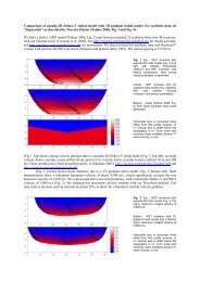
4.1.1 Traveltime Field Computation 

Traveltime field computation serves as quality control of depth-velocity models 

as obtained with Delta-t-V method by forward modelling of wave propagation 

through these models. Figure 4.1 shows the shot break windows 

within Rayfract illustrating the differences between modelled and measured 

traveltimes after 10 and 50 iterations. Modelled traveltimes are coloured blue 

while measured lines are black. Here the measured traveltimes are synthetically 

created traveltimes. 

Figure 4.1: Shot break windows illustrating the differences between modelled (blue) and 

measured (black) traveltimes after 10 (top) and 50 (bottom) iterations. It can easily be seen, 

that several iterations yield better agreement of the curves. 

The forward modelling algorithm is the first-order Eikonal solver, which calculates 

traveltimes of the fastest wave at any point of a regular grid, including

Delta-t-V Inversion 21 

head waves (Podvin and Lecomte, 1991). 

Refraction seismology is mostly based on traveltime interpretation and this 

algorithm is capable of finding both, traveltimes and raypaths (Lecomte et al., 

2000). Ray tracing can be used to obtain an estimate of the arrival time, but 

in classical approaches a layer must have a vertical velocity-gradient in order 

to simulate critically refracted rays back-propagating to the surface. Vidale 

(1988) proposed a very efficient method to calculate traveltimes on a regular 

velocity grid by solving the Eikonal equation using finite differences. This 

type of solution is called an Eikonal solver (Lecomte et al., 2000). 

The potential of the Eikonal solver in refraction seismic, both for modelling 

of traveltimes and inversion, has been shown by Aldridge and Oldenburg 

(1992), who used a modified version of Vidale’s (1988). They demonstrated 

how to apply the refractor-imaging principle of Hagedoorn (1959)(disussed 

in Appendix B), which requires back-propagation of the wavefronts associated 

with head waves. Their major problem was the restriction to a plane 

topography of the recording surface. This limitation has been overcome by 

Podvin and Lecomte (1991) by using a more flexible Eikonal solver algorithm 

based on Vidale (1988). 

S’’ 

O 

● 

○ 

P 

h 

S 

S’ 

● 

M 

● 

N 

(a) Local Scheme 

(b) Expanding/contracting square ring 

process 

Figure 4.2: (a) Local Scheme with three known traveltimes (t M , t N , t O ) for finding the 

fourth (t P ). Segments [MN], [MO] are plane wave estimators. A diffraction generated from 

M and two surface waves are calculated from the traveltimes at O and N. (b) The expanding/ 

contracting square ring process with point source in centre. When surface waves are generated 

along a side of the ring, potential back-propagating head waves are examined by contracting 

the ring from the respective side. (Lecomte et al., 2000)


Vidale (1988) obtained the Eikonal equation from the elastic-wave equations 

by searching for plane harmonic solutions and applying the high-frequency 

approximation of ray theory. In two dimensions this is: 

( ) 2 ( ) 2 ∂T ∂T 

+ = s 2 , (4.1.3) 

∂x ∂z 

where T is i.e. the traveltime of the wave with slowness s. 

Vidale solved equation (4.1.3) by using finite differences to estimate the partial 

derivatives. Considering the lower left square of figure 4.2a traveltimes 

are calculated within regular grids where the traveltimes at three out of the 

four corners are known (t M , t N and t O ) and the fourth (t P ) is found by applying 

the equation he derived (see section A in the Appendix). This equation 

(see eq: (A.0.1)) has some limitations and a major problem of this algorithm 

is that the local scheme is applied without considering the surrounding slowness 

structure. 

Podvin and Lecomte (1991) chose an approach where they used the regular 

grid slowness representation as a physical representation, i.e. the actual 

slowness model is approximated by a model with square cells of constant 

slowness. Using the local scheme in figure 4.2a with a wavefront passing 

point M first, they found five estimators for the traveltime from which the 

smallest is kept. 

t P = t N ± √ (hs) 2 − (t N − t M ) 2 

for 0 ≤ t N − t M ≤ hs √ 

2 

(4.1.4) 

t P = t O ± √ (hs) 2 − (t O − t M ) 2 

for 0 ≤ t O − t M ≤ hs √ 

2 

(4.1.5) 

t P = t M + √ 2hs (4.1.6) 

t P = t N + hmin(s, s ′ ) (4.1.7)

Smooth Inversion 23 

t P = t O + hmin(s, s ′′ ). (4.1.8) 

Here all sides of the cell have the same length, h, and the limits in equations 

(4.1.4) and (4.1.5) take the angle of the incoming wavefront into account; 

that is a rather steep wavefront passing first point M, then point O followed 

by the centre of the cell leads to the use of equation (4.1.5) while equation 

(4.1.4) does not fulfill the limit criteria. 

In spite of these five estimators, it still makes sense to use Vidale’s equation 

instead of equations (4.1.4), (4.1.5) and (4.1.6) as long as the argument 

of the square root of equation A.0.1 in Appendix A is not negative. 

Head waves propagating along the outer part of one of the cell sides are 

represented by traveltime estimators (4.1.7) and (4.1.8). As the head waves 

initiate wavefronts which may return to previous calculated zones Podvin 

and Lecomte (1991) introduced an expanding/contracting square ring process 

(figure 4.2b). From the source point, in the centre of the square, traveltimes 

are determined along successive square rings using traveltimes from the 

previous ring. When the two mentioned estimators are used along a side of 

the current ring, potential head waves are examined by contracting the ring 

from the respective side until no more traveltimes are updated (decreased). 

Systematic application of the estimators, which only use traveltimes on the 

previous ring, reveals the smallest traveltime. Then estimators, which use 

only one point on the previous ring and one on the current ring, are applied 

in one direction followed by the other direction. A recursive process will follow, 

if the interface wave estimator has minimized a travetlime. 

Other methods have been developed as well, but they are not as efficient 

as the described square ring process and shall not be elaborated here. For 

further reading refer to Lecomte et al. (2000). 

4.2 Smooth Inversion 

Smooth Inversion uses, as mentioned above, the result of theDelta-t-V Inversion 

method and generates a 1D-gradient initial model. The Pseudo-2D 

Delta-t-V initial model, obtained with Delta-t-V Inversion, results in an indi-


vidual velocity vs. depth profile below each profile station. Smooth inversion 

averages the obtained velocities over all profile stations at common depths 

resulting in an average velocity vs. depth profile. This average velocity vs. 

depth profile is then extended laterally along the whole profile. A 1D gradient 

velocity grid is generated based on these average velocities (Rohdewald, 

1999). Smooth inversion automatically starts the subsequent WET Wavepath 

Eikonal Traveltime Inversion with the default parameters and settings. 

4.3 WET Wavepath Eikonal Traveltime tomography 

The limitation conventional ray tracing tomography faces, modelling of just 

one ray per first break, has been overcome by Rayfract by using WET 

Wavepath Eikonal Traveltime tomography, in the following just called WET. 

WET models multiple signal propagation paths contributing to one first 

break. Wavepaths are based on Fresnel volumes, also known as fat rays 

(treated in section 4.3.1), which take the band-limited effects of the source 

wavelet and the diffraction effects into account. 

The used WET code has been developed by Schuster and Quintus-Bosz 

(1993) and is based on a finite-difference solution to the Eikonal equation 

(Schuster, 1991). When scattering effects are dominant or the characteristic 

scale of the medium is about the same as or smaller than the dominant source 

wavelength, this principle is invalid. 

The starting-point is the general formula for the back projection of traveltime 

or phase residuals: 

γ(x) = 2s(x)A rs∆t 

A xr A xs 

∫inf 

−inf 

ω 3 ˜Rrs (ω) × sin(ω[t xs + t xr − t rs ]) dω (4.3.1) 

with t xs and t xr the first-arrival traveltime solution to the Eikonal equation 

for a receiver at x r and source at x s , in a slowness distribution s(x); A xs is 

the associated geometrical spreading term of the first arrival, whose reciprocal 

satisfies the transport equation; ˜Rrs is an arbitrary weighting function, 

which main effect it is to smooth the gradient (or reconstruct the slowness

WET Wavepath Eikonal Traveltime tomography 25 

field) in a way that is consistent with the source spectrum and the path propagation. 

Scattering effects in the data are ignored as the phase is linearized 

with respect to frequency. Equation (4.3.1) is derived from the phase misfit 

function 

ɛ = 1 2 

∑ ∑ ∑ 

s r ω 

˜R rs (ω)∆φ(x r , x s , ω) 2 , (4.3.2) 

with the summation over the receivers r and sources s and over the discrete 

source frequencies ω. ∆φ(x r , x s , w) is the phase residual, which is determined 

as the difference between the calculated and observed phases of the first 

arrivals at a single frequency. 

The gradient of ɛ with respect to the slowness yields the gradient of the phase 

misfit. With this the slowness can be reconstructed. Implementing several 

definitions, substitutions and linearization of phase with respect to the firstarrival 

traveltime finally yields equation (4.3.1). 

Applying this equation by substituting certain expressions for the weighting 

function, ˜Rrs , leads to different tomography methods including the WET 

equation, which will be shown in the following. 

Considering the case of an inhomogeneous medium, a narrow-band source 

with a center frequency ω c and a bandwidth 2ω 0 , setting ˜R rs (ω) to 1 / 2 , and 

replacing the integration by 

−ω∫ 

c+ω 0 

−ω c−ω 0 

dω + 

ω∫ 

c+ω 0 

ω c−ω 0 

dω, (4.3.3) 

and assuming an ω-value close to zero yields: 

γ(x) = 4ω 0s(x)A rs ∆t 

A xr A xs 

( 

× sinc ′′′ ω0 

) 

π (t xs + t xr − t rs ) . (4.3.4) 

The triple prime indicates the triple differentiation with respect to the argument. 

Traveltime residuals are back-projected into the medium along ’sincpaths’ 

(rather than raypaths) and weighted along surfaces of constant phase


or traveltime (Schuster and Quintus-Bosz, 1993). 

Replacing ˜R rs (ω) in equation (4.3.1) by the magnitude spectrum of i.e. a 

Ricker wavelet 1 replaces the triple derivative sinc-function by the time domain 

Ricker wavelet W ′′′ (t xs + t xr − t rs )/2ω 0 . The asymptotic gradient for 

the WET inversion is then (Schuster, 1991, Quintus-Bosz, 1992): 

γ(x) = 2s(x)A rs∆t 

A xr A xs 

W ′′′ (t xs + t xr − t rs ). (4.3.5) 

With this equation the wavepath is shaped by the magnitude spectrum of the 

source wavelet, which is physically consistent with the actual path of wave 

propagation for a shifted zero phase wavelet. 

After the first-arrival traveltimes, t obs 

rs , have been picked from seismograms 

the numerical algorithm for WET inversion is: 

ˆ to propose an initial slowness model and solve the Eikonal equation by 

a finite difference method (Qin et al., 1992) to get t xs and t xr . The 

traveltime residual ∆t = t rs − t obs 

rs is computed. t rs are the finitedifference 

traveltimes. 

ˆ to evaluate source weighting function in equation (4.3.5) at all points 

in the medium yielding γ(x). In practice, summation over source and 

receiver positions are included in order to take multiple sources and 

receivers into account. 

ˆ to update the slowness model and repeat the steps iteratively until convergence. 

This scheme has been successfully tested for its effectiveness 

by Quintus-Bosz (1992). 

1 Ricker wavelet is the negative normalized second derivative of at Gaussian function. 

It is defined by the input parameters “wavelet reference (center) 

time”, t 0 , and “maximum amplitude frequency”, f m , with the respective 

units seconds and Hz. In analytical form they are used in 

) 

with the spec- 

) 

W (t) = 

(1 − (2πfm(t−t0))2 

2 

exp 

( ( 

trum S(ω) = 4√ πω 2 

(2πf m) 

exp − 

3 

(− (2πfm(t−t0))2 

4 

ω 

2πf m 

) 2 

) 

exp(iωt 0 ). 

It is also known as the“Mexican hat wavelet”which becomes clear 

when looking at its curve as illustrated in the figure on the right.

WET Wavepath Eikonal Traveltime tomography 27 

4.3.1 Fresnel volume - Fat Rays 

Geometric ray theory is commonly used in seismic imaging. It is an asymptotic 

solution of the wave equation in the high-frequency limit. It includes 

the assumption that waves propagate along infinite narrow lines, rays, joining 

the source and receiver (Spetzler and Snieder, 2004). Infinite narrow lines 

correspond to infinite frequencies, which is not the case for waves recorded 

in reality as their frequency content is finite. Limiting the frequency band of 

waves implies that their propagation is extended to a finite volume around 

the geometrical ray path. This volume is called the Fresnel volume. 

Husen and Kissling (2001) define the Fresnel volume of a seismic wave as the 

innermost spatial region where constructive interference of seismic energy 

takes place. Hence, scattering from each point within the Fresnel volume 

contributes constructively to the signal observed at a receiver. 

Solving the Eikonal equations directly guarantees that the global minimum 

traveltime is found (Husen and Kissling, 2001). 

Summation of both travel time 

Receiver 

∇ 

fields, the forward and the backward 

propagating waves, yields the 

t sx +t rx -t sr =T/2 

fat ray (Fig. 4.3) representing the 

● x 

wave path from the source to the 

receiver. 

The traveltime fields of both 

the forward and backward waves 

Source 

are calculated using the finitedifference 

algorithm as described in 

t sx +t rx -t sr =0 

* 

chapter 4.1.1. The width of the Figure 4.3: Diagram of the fat ray concept. 

Fresnel volume is defined by Cerveny 

and Soares (1992) in terms 

Source and Receiver travel time are computed using 

finite-difference modelling. Their summation 

is used to define a fat ray, given those points with 

of travel times t sx , t rx between a summed travel time less than t sr + T/2. 

the source and the receiver respectively, 

and a point x within the Fresnel volume as 

|t sx + t rx − t sr | ≤ T/2 (4.3.6) 

where T is the dominant period of the seismic wave and t sr the shortest 

traveltime between source and receiver. The width of the fat ray should be 

defined by the points resulting from the equality of equation (4.3.6) in order


to correctly represent the first Fresnel volume. For example, for a dominant 

frequency of 50 Hz the ideal fat ray width should correspond to points 

having a 0.01 s traveltime difference. With a refractor of uniform velocity 

v 2 equal to 5000 m/s and an overburden velocity v 1 of 500 ms the corresponding 

minimum fat ray width of 100 m within the refractor, and 10 m in 

the overburden, is obtained. In areas of higher velocities the fat ray tends to 

broaden, which is an expected behaviour of Fresnel zones. 

A more theoretical approach is described by Spetzler and Snieder (2004).

Chapter 5 

Investigations 

For the following investigations the version 3.16 of the tomographic inversion 

tool Rayfract is used. 

In order to understand the capabilities the Rayfract code has to recognize 

anomalies of different dimensions, locations and properties, a rather thorough 

sensitivity investigation is necessary to start this work. 

A description of how synthetic traveltimes are created is followed by an 

overview of the models designed for computing the first arrival traveltimes. 

Then the outcome of the sensitivity investigation is shortly described. The 

result of this investigation decides the choice of the model for the subsequent 

parameter investigation. In this chapter all for the inversion relevant settings 

and parameter options are stated. The results, which have the desired 

positive impact on the inversions, are discussed in chapter 6, where different 

combinations of the findings are presented as well. 

5.1 Sensitivity Investigation 

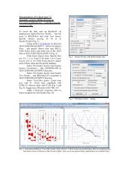
Synthetic traveltimes are computed by the program using its built in Eikonal 

solver. 

The procedure is to import a set of random traveltimes in form of an ASCIIfile, 

which contains shot positions, receiver positions and first arrival travel-

30 Investigations 

times. The number of receivers and shots should correspond to the desired 

set-up. A Delta-t-V Inversion is run, which creates a set of files including the 

grid-file DELTATV.GRD, which dictates the frame for the synthetic model; 

amongst others it states the borders, number of grid-points and spacing between 

points to be used for the model. The synthetic models have been 

created with Golden Software Surfer 1 . When conducting the forward modelling 

traveltimes, which is an option within the menu-item WET Tomo 2 , 

the created model is imported for the computations. Modelled traveltimes 

are then exported to an ASCII-file, which contains the first arrival traveltimes 

of the synthetic model. 

Here two sets of data densities are created for nearly all synthetic models. 

One set of traveltimes is with 48 receivers and 25 shots, with a shot at every 

second receiver; the other set corresponds to a field setup and consists of two 

spreads, each with 24 receivers, and the source at every sixth receiver (figure 

5.1). This comparison reveals the quality of inversions with a sparse data set 

compared to a dense data set. 

It shall be mentioned that all inversions are run with 50 iterations instead of 

the default 10 iterations 3 . As stated by the software developer and verified 

in pre-studies increases the image contrast with an increased number of iterations. 

Fifty iterations is rated as a reasonable choice with respect to inversion time 

and image quality. 

Figure 5.2 illustrates the development of the absolute RMS-error and maximum 

absolute error versus numbers of iterations for the inversion set-up 

PARRES 1 as discussed in section 6.3. Maximum absolute error is the error 

for a certain trace and shot number. 

1 Any other software, which is capable of creating a grid-file (grd.-file), can be used as 

well. 

2 In version 3.18 this function is located in the menu point ”Model” and the generation 

of synthetic traveltimes is simplified as the Delta-t-V Inversion is no longer needed. 

3 For narrow shot spacing (here the set-up with 48 geophones and 25 shots) the default 

is 20 iterations and for wide shot spacing (here the set-up with 2 × 24 geophones and 2 × 

6 shots) the default is 10 iterations.

Time [ms] 

Sensitivity Investigation 31 

G1 G2 G3 G4 G47 G48 

▼ ▼ ▼ ▼ ▼ ▼ 

★ ★ ★ ★ 

S1 S2 S24 S25 

at G49 

G23 G24 G25 G45 G46 

▼ ▼ ▼ ▼ ▼ 

G1 G2 G3 G23 G24 

▼ ▼ ▼ ▼ ▼ 

★ ★ ★ ★ ★ 

S1 

S4 / S7 

S5 / S8 S6 / S9 

S12 

at G19 

at G25 at G31 

at G49 

Figure 5.1: Illustration of the used source-receiver set-ups for the sensitivity investigation. 

The upper part shows the set-up for a spread with 48 geophones and 25 shots, one at every 

other geophone position. The lower sketch shows a set-up with two spreads, each with 24 

geophones, and six shots per spread. The two spreads overlap with two geophone positions 

and three shot positions. First two geophones of the second spread are numbered 23 and 24 

as their position is equal to the last two geophones of the first spread. This way of numbering 

is important for the processing. 

1,2 

1 

absolute RMS error [ms] 

Maximum absolute error [ms] 

0,8 

0,6 

0,4 

0,2 

0 

0 100 200 300 400 500 

Number of Iterations 

Figure 5.2: Development of the absolute RMS and maximum error in steps of 10 for up to 500 

iterations. A minimum of the absolute RMS-error is reached after 140 iterations whereupon 

it stays constant. The maximum absolute error reaches its minimum after 200 iterations and 

increases slowly before it jumps in parallel with the absolute RMS-error in the last iteration. 

This behaviour is explained in the text.


A minimum of the absolute RMS-error is reached after 140 iterations whereupon 

this value stays constant. The maximum absolute error reaches its 

minimum after 200 iterations, thereafter its value increases slowly. 

The explanation for this is, that the maximum absolute error originates from 

a certain shot and trace number and varies or can vary for each iteration. 

Starting with iteration 200, the same trace causes the largest absolute error 

up to iteration 499. An increase of the error means that the inversion output 

becomes less dependent on this trace (Rohdewald, 2010). At the last iteration 

the increase of 0.02 ms originates from a different shot and trace number. 

With this increase a simultaneous increase of the absolute RMS-error follows 

as the maximum absolute error is part of its computation. 

It shall be noted that this example deals with synthetically modelled traveltimes 

and errors are marginal, therefore it is not necessary to run such a 

high number of iterations. However, when working with data from field measurements 

an examination of these errors can help to obtain a more reliable 

result. 

5.1.1 Synthetic Models 

For each subsurface structure a synthetic model was designed. All together 

27 models were created. The build up of these models is: 

ˆ velocity gradient: 1000 m/s at top, increasing with 50 m/s per metre, 

and anomalies 

– of 5 × 5 m 2 and 2 × 2 m 2 with a constant velocity of 5000 m/s, 

– in different locations within the layer: centre, lower centre, upper 

centre, middle left, upper left and lower left. 

– of 5 × 5 m 2 with constant velocity of 3000, 2000 and 1500 m/s. 

ˆ overburden with above velocity gradient and a constant refractor velocity 

of 5000 m/s and 

– 10 × 10 m 2 and 5 × 10 m 2 anticlines in the lower centre, lower 

left. 

– 10 m wide synclines penetrating into the refractor.

Sensitivity Investigation 33 

ˆ overburden with above velocity gradient and a constant refractor velocity 

of 1000 m/s and 

– 10 × 10 m 2 anticline in the lower centre 

ˆ vertically divided area, left side above velocity gradient and 

– right side with a higher velocity gradient 

– right side with a constant velocity of 5000 m/s 

ˆ overburden with above velocity gradient, an opening of 100 m in the 

refractor and 

– a constant refractor velocity of 2000 m/s 

– a constant refractor velocity of 5000 m/s 

ˆ Overburden of 5 m thickness and above velocity gradient, constant 

refractor velocity of 5000 m/s and 

– rift with 10 m opening at interface and 15 degree dipping angle 




ˆ Overburden of 5 m thickness and above velocity gradient, refractor 

velocity gradient with 4000 m/s at interface, increase of 40 m/s per 

metre and 



Illustrations of all synthetic models can be found in Appendix C. 

5.1.2 Results of Sensitivity Investigation 

In this section a resumé of the outcome of the sensitivity investigation is 

given. 

For anomalies with larger velocities than the surroundings the code has no


problem in modellinig them, neither the 5 × 5 m 2 nor 2 × 2 m 2 anomalies. 

Different locations in the subsurface are recognized as well. But the 

same box-shaped anomalies are not recognized by the inversion when their 

velocities are equal to or smaller than their surroundings (see figure C.19). 

However, an anomaly of larger dimension and in connection with the low 

velocity refractor is discovered by the code (see figure C.12). 

These results show clearly that the set-up used in field surveys (sparse shot 

and receiver coverage as shown in figure 5.1) is sufficient for being used for 

the parameter investigation (see figures in Appendix C). 

Dipping faults with an opening of 10 m at the interface compose some difficulties. 

Neither the 15 nor the 75 degrees rift is modelled by the inversion; 

both are modelled as vertical structures. However, with a larger opening 

(here 38 m) the code is capable of modelling an angle, though not the original 

15 degrees, which is the only model tested with this opening. 

In order to see, if there are traveltime differences for different dipping angles, 

an examination of their first arrival traveltimes is carried out. Times 

for a plane structure (0 degree) and dipping angles of 15, 75 and 90 degrees 

are directly compared by subtracting them from each other. 

Figure C.28 illustrates the obtained time differences in % with the CMP in 

station-numbers as x-axis and the offset in station-numbers as y-axis. Differences 

of first arrival traveltimes between various dipping angles can be 

observed. With larger differences between the dipping angles the time differnces 

increases as well. This could be caused by the fact that for rifts with 

larger angles the wavepaths travel a longer distance in the low velocity zone 

of the rift. 

But, are the respective angles of the models disclosed by these plots, too? 

In the first three sub-figures, where the traveltimes for the plane structure 

is subtracted from traveltims for the dipping structures, the time differences 

are very symmetric, which means that the differences in dipping angles are 

not revealed. The same symmetry is the case in the fourth sub-figure (figure 

C.28d). The time difference for the last case does not show this symmetry, 

which proves, that rifts with different dipping angles and an opening of only 

10 m at the same offset are modelled by the code, and not only the opening. 

Here, time differences of more than 10 % are modelled.

Parameter Investigation 35 

5.2 Parameter Investigation 

As a consequence of the sensitivity investigation one model was chosen for 

the following parameter investigation. Criterion for the chosen model was 

that it, as much as possible, should conform with realistic subsurface geologies. 

As the most suited model for the investigation model Ub, as shown in 

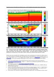
Figure 5.3a, was selected. Figure 5.3b illustrates the tomogram obtained for 

default settings and parameters. Grey dots mark the receiver stations and 

red triangles the shot positions. 

(a) Model U 

(b) Tomogram for model U 

Figure 5.3: (a) Model for the parameter investigations. The velocity gradient of the overburden 

starts with 1000 m/s at the surface and increases with 50 m/s per metre; it continues 

into the anomaly through the hole of 10 m width. The anomaly has a constant velocity of 

5000 m/s. (b) Tomogram for model U with two spreads of 24 geophones (grey dots) and 

six shots (red triangles) per spread. Two receiver positions and three shot positions overlap. 

Default settings and parameters are used. The resulting absolute and normalized RMS-errors 

are 0.17 ms and 0.3 % respectivley. The x-axis states the offset and the y-axis the altitude, 

both in metres.


Its associated RMS-error is 0.17 ms, which corresponds to 0.3 % for the normalized 

RMS-error. Figure 5.4 illustrates the wavepath coverage belonging 

to this tomogram. 

Figure 5.4: Wavepath coverage to the tomogram in figure 5.3b in number of wavepaths per 

pixel. 

Only the case, which corresponds to a field measurement set-up, 2 × 24 geophones 

with 2 × 6 shots, was used for the investigations as the sensitivity 

investigation showed this to be sufficient, and with future applications in 

mind. 

In order to see the influence of each setting and parameter individually only 

one at a time was changed compared to default. After all possibilities were 

tested, the ones, which deliver improved RMS-errors compared to the reference, 

are combined in the same inversion. This led to several combination 

possibilities, which gave reasonable improved results. 

As mentioned above there are two options for generating initial gradient 

models for the WET tomography. One is the Delta-t-V Inversion which, 

according to the SW-provider, leads to artefacts in synclines and anticlines. 

The other is Smooth Inversion, which creates a quasi-horizontal subsurface 

layering based on the Delta-t-V Inversion. According to the SW-provider 

it guarantees a realistic interpretation and velocity artefacts from Delta-t- 

V Inversion are virtually eliminated. Figure 5.5 illustrates initial models 

generated with both options. The difference between these model is obvious.


Figure 5.5: Example of the difference between an initial model generated from Smooth 

Inversion (left) and Delta-t-V Inversion (right). 

In this investigation all initial models were created with the Smooth Inversion. 

As the Delta-t-V Inversion is the basis for the Smooth Inversion, its 

parameters do have an impact on it, therefore they are tested as well. As 

the last step the WET Tomography Inversion refines the initial model and 

creates a tomogram of the subsurface. As for the sensitivity investigation all 

inversions were run with 50 iterations. 

The following sections treat each part, Smooth Inversion, Delta-t-V Inversion 

and WET Tomography, separately describing the applied options and 

parameters. The inversion results are discussed in chapter 6. For evaluating 

the quality of the inversions, which is challenging when comparing tomograms, 

the absolute and normalized RMS-error, as directly calculated by the 

SW, were used. Nonetheless, an examination of the modelled velocities is 

conducted, too. 

5.2.1 Smooth Inversion Settings 

As this inversion is based on the Delta-t-V Inversion, there are not many 

possibilities to influence its settings. No parameters can be set, but there are 

some options to check and un-check. These options are: 

ˆ Lower velocity of 1D-gradient layers: 

Should be activated when obtained velocities seem too high. Disabled 

per default.


ˆ Interpolate velocity for 1D-gradient initial model: 

Self explanatory. Checked per default. 

ˆ Output inversion results in feet: 

Self explanatory and not actual here. 

ˆ Strict shot position checking: 

Self explanatory. Disabled per default. 

Options not active/accessible are not mentioned. Output inversion results in 

feet is not tested as only metric units are considered. 

5.2.2 Delta-t-V Inversion Settings and Parameters 

As mentioned before, the Delta-t-V inversion was not used for the creation 

of the initial model. But as the Smooth Inversion applies its parameters and 

settings they are tested as well. The General Delta-t-V Settings are: 

ˆ Output Measured CMP velocities: 

When activated inverted velocities and depths are combined with measured 

velocities at corresponding source-receiver offsets. When not active 

velocities are only based on inverted velocities. Default is not active. 

ˆ Output Horizontal offset of CMP pos. in meters: 

Checked per default. Non-active option results in the unit feet. 

ˆ Output Delta-t-V results in Feet: 

Self explanatory and not actual here. Un-checked per default. 

ˆ CMP is zero time trace: 

Adds a first break data point with time 0 at offset 0 of the CMP traveltime 

curve. Checked per default. 

ˆ Reduced offset 0.0 is valid trace with time 0.0: 

Enabled ensures the fullest use of information in near-offset part of 

CMP sorted and stacked traveltime curves. Active by default; should be 

de-activated when output too noisy.


ˆ Enforce Monotonically increasing layer bottom velocity: 

Self-explanatory. Not active per default. 

ˆ Suppress velocity artefacts: 

When active the generation of unrealistic velocity variations is suppressed. 

Best for medium and high coverage profiles. Per default not 

enabled. 

ˆ Process every CMP offset: 

When active a better vertical resolution is obtained, but an increased 

amount of artefacts might be obtained. Default is disabled. 

ˆ Prefer Average over minimum interface velocity: 

When enabled the capability of high velocity anomaly imaging in the 

near surface region is enhanced. Disabled it enhances the low velocity 

imaging capability of the Delta-t-V inversion. Recommended to leave 

enabled in case of strong lateral velocity variation. Default is enabled. 

ˆ Taper velocity steps at layer interface: 

Enabled it may result in an enhanced vertical resolution of subsurface 

layer interfaces, in case of subhorizontal layering and for high coverage 

surveys (e.g. 15 or more shots per profile). The resulting model will 

be slightly too deep i.e. too slow, in most situations. Recommended 

to leave this option disabled in case of strong lateral velocity variation. 

Not active per default. 

ˆ Smooth CMP traveltime curves: 

To be used for high coverage profiles only. May help to filter out bad 

picks from CMP sorted and stacked traveltime curves. For low coverage 

profiles, enabling this option may result in the destruction of valuable 

vertical gradient information. Not active per default. 

ˆ Weigh picks in CMP curves: 

Picked traveltime curves are weighted. Checked per default. 

In Interactive Delta-t-V several options and parameters can be chosen. This 

area is subdivided into group-windows. The main window, Parameters for 

Delta-t-V method, contains the following parameters: 

ˆ CMP curve stack width [CMPs]: 

Specifies the number of CMP positions for constructing the CMP traveltime 

curve. Ranges from 10 to 25 CMP s.


ˆ Regression over offset stations: 

Specifies the length of the offset interval for local piecewise linearization 

of CMP traveltime curves. A smoothed local apparent CMP velocity is 

obtained. Small values deliver shallower velocity-depths model, therefore 

for low coverage surveys values close to the minimum should be 

chosen. Ranges from 5 to 20 and the linear regression method is chosen 

in the option below. 

ˆ Linear regression method: 

– least squares: Local apparent CMP traveltime curve velocities are 

determined with an offset interval of length ’Regression over offset 

stations’ and centered at the offset currently evaluated. Active per 

default 

– least deviations: This method recognizes outliers and less relevant 

dats points and weighs them less when modelling. 

ˆ Weathering sub-layer count: 

For controlling weathering velocity in situations of strong possibly nonlinear 

vertical velocity gradients right below topography. Values range 

from 0 to 1000 and default is 3. High values yield lower traveltimes. 

When synthetic traveltimes are too fast this value should be increased. 

ˆ Maximum valid velocity: 

Limits the maximum velocity of the model to the specified value. 

ˆ Process all CMP curves: 

– process all CMP 

– skip every 2nd 

Two push buttons, named Static Corrections and Export Options, open new 

windows. Window Static Corrections contains the following possibilities: 

ˆ What static correction 

– No static corrections applied: 

In situations of flat topography or topography approximating a dipping 

plane. First breaks are still corrected for shot position offsets 

and shot hole depth. These corrections need near-surface weathering 

velocity, which is determined with the parameter “Weathering 

crossover” (see below).


– Surface consistent corrections: 

Static first break corrections relative to a floating datum obtained 

by applying a running average smoothing filter. Filter width is 

specified in field “Topography filter” (see below). 

– CMP Gather datum specific: 

First break static correction relative to a dipping datum plane specific 

to the CMP gather. The datum plane is obtained by linear regression 

of all sources and receivers connected to the actual CMP. 

ˆ Determination of weathering velocity 

– Copy v0 from Station editor: 

Reuses weathering velocities specified in Station editor. Not actual 

here. 

– Automatically estimate v0: 

Force estimation of a general laterally varying near-surface velocity 

based on the laterally constant crossover distance “Weathering 

crossover”. This option is active per default. 

ˆ Station number intervals [station nrs.] 

– Weathering crossover: 

Specifies the laterally constant estimated average crossover distance 

separating direct wave-arrivals from refracted arrivals. 

– Topography filter: 

Specifies the filter width for the running average filter applied to 

topography to obtain a smoothed floating datum. 

ˆ Trace weighting in CMP stack [1/stat.nrs.] 

– Inverse CMP offset power: 

Weighs individual traces in one CMP stack based on the actual 

CMP offset from the central CMP. Default value is 0.5 and decrease 

of it gives more weight to large CMP offsets. This option is 

active by default and the default value is kept for all investigations. 

Options and parameters within the window Export Options are not tested 

and therefore not mentioned here. Only the option Maximum velocity exported 

influences the generation of the initial model; the default value of this 

parameter is kept.


5.2.3 WET Tomography Inversion Settings and Parameters 

General Settings which can be checked/un-checked are listed below. Most 

functions are clear from their name and do not need further explanation; 

where necessary the purpose of the function is explained. 

ˆ Write grids for every iteration: 

No effect on the inversion itself. 

generated. 

After each iteration a grid-file is 

ˆ Update imaged grid depth: checked per default 

ˆ Adjust wavepath width: 

Enabled WET determines the wavepath width for each trace individually. 

Improved overburden resolution and more smoothing/less artefacts 

in the basement are ensured. When disabled the constant wavepath 

width (see ”Interactive WET tomography”) is used. For profiles with 72 

or more receiver stations this option is enabled per default. 

ˆ Scale WET filter height: 

Scales smoothing filter height with depth below topography. Ensures 

better vertical resolution of weathering layer and fewer artefacts at the 

bottom of WET tomograms. For profiles with 72 or more receiver stations 

this option is enabled per default. 

ˆ Blank low coverage after each iteration 

ˆ Blank low coverage after last iteration 

ˆ Blank below envelope after each iteration 

ˆ Blank below envelope after last iteration: checked per default 

ˆ Interpolate missing coverage after last iteration 

ˆ Disable wavepath adjustment for wide shot spacing: checked per default 

ˆ Reset WET tomography setting to default


Interactive WET tomography has the following options: 

ˆ Number of WET tomography iterations: 

Specifies the number of WET tomography iterations. Default is 10 i- 

terations (see footnote 3 on page 30). All investigations are performed 

with 50 iterations. 

ˆ Central Ricker wavelet frequency: 

Central frequency of the Ricker wavelet used to modulate the wavepath 

misfit gradient amplitude. Default value is 50 Hz which is kept during 

the investigations. 

ˆ Degree of differentiation of Ricker wavelet: 

This number specifies how many times the Ricker wavelet should be 

differentiated. Recommended to keep the default value of 0 resulting in 

a more robust tomographic inversion and fewer artefacts. 

ˆ Wavepath width [percent of one period]: 

Specifies the wavepath width in percent of one period of the Ricker 

wavelet central frequency. Ranges up to 10 % (and 100 % in version 

3.18). Increased value corresponds to wider wavepaths and smoother 

velocity models. 

ˆ Envelope wavepath width [percent of period]: 

Specifies the width of the wavepaths used to construct the envelope at 

the bottom of the tomogram. Recommended value is 0, its maximum 

possible value is 0.1 % smaller than “Wavepath width”. 

ˆ Maximum valid velocity [m/sec.]: 

Specifies the maximum valid velocity when processing CMP curves and 

overrides the specified value of Interactive Delta-t-V maximum valid 

velocity. Velocities exceeding this threshold are reset to the specified 

value.


Furthermore there are the push buttons named Edit velocity smoothing and 

Edit grid file generation. Options within Edit velocity smoothing are: 

ˆ Full smoothing after each tomography iteration: 

Results in smoother tomograms. Recommended for the first (i.e. first 

ten) WET iterations. This option is chosen per default. 

ˆ Minimal smoothing after each tomography iteration: 

Results in tomograms with more details. Recommended for the last few 

(i.e. last ten) WET iterations. 

ˆ Manual specification of smoothing filter. These specifications are the 

Smoothing filter dimensions 

– Half smoothing filter width: 

Number of columns scanned on each side of the current cell. 

– Half smoothing filter height: 

Number of rows scanned above and below the current cell. 

ˆ Filter shallow dipping wavepath artefacts from model 

– Automatically adapt shape of rectangular filter matrix: 

Suppresses artefacts. Recommended to leave checked. 

ˆ Maximum relative velocity update after each iteration 

– Maximum velocity update: 

Specifies the maximum allowed relative update of each velocity 

model cell after each iteration. Updates will be limited by this 

threshold. Per default this value is set to 15 % and it ranges from 

5 % to 35 %. 

Options within the push button Edit grid file generation do only have impact 

on the files generated after each iteration and not on the tomographic 

inversions. Therefore no inversions for examining them are carried out and 

they are not elaborated any further.

Chapter 6 

Results of the Parameter 

Investigations 

In this chapter the settings and parameters, which have a positive impact on 

the inversion results for the synthetic traveltimes computed from model Ub, 

are discussed. This means, only inversions with reduced absolute/normalized 

RMS errors are discussed. An overview of the remaining tomograms and their 

respective RMS-errors can be found in Appendix D. 

6.1 Smooth Inversion 

6.1.1 Smooth Inversion Settings 

From all possible settings within Smooth Inversion the options Lower velocity 

of 1D-gradient layers activated, and Interpolate velocity for 1D-gradient 

initial model deactivated, yield lower RMS-errors compared to the reference. 

In the first case an absolute RMS-error of 0.16 ms and in the second case of 

0.15 ms, which corresponds to an improvement of 0.01 ms (6 %) and 0.02 

ms (12 %) respectively, is obtained. Table 6.1 gives an overview of all results 

and figure 6.1 shows their tomograms.

46 Results of the Parameter Investigations 

In table 6.1 an overview of the obtained inversion results is shown. 

Smooth Inversion Setting option RMS-error 

Default Settings 

0.17 ms 

Lower velocity of 1D-gradient layers activated 0.16 ms 

Interoplate velocity for 1D-gradient de-activated 0.15 ms 

initial model 

Strict shot position checking activated 0.17 ms 

Table 6.1: 

iterations. 

Smooth Inversion settings with respective absolute RMS-error after 50 WET 

The difference in absolute RMS-error seems small and at first glance their 

tomograms are almost identical with the reference. 

Taking a closer look at the contour-lines reveals a difference in altitude compared 

to the reference model. In the upper tomogram the contour line for 

1500 m/s is located at about the 90 m mark while it is above this mark in the 

reference model. This agrees very well with the synthetic model which has 

exactly the same velocity at this altitude. Reaching the anomaly, at about 

81 m, does not show any difference, but beneath a slight uplift of the 4500 

m/s line is observed. Both the 1500 and 4500-line are indications of causing 

the decrease of absolute RMS-error. 

In the lower tomogram the 1500-line is moved further below the 90 m mark. 

This is worse compared to the synthetic model. Looking at the area below 

the intersection, a further increase of the velocity is revealed in the lower 

half-space. The 4500-line is lifted up to about 77 m. 

Activating the option Strict shot position checking yields exactly the same 

inversion result as the default settings. Since the task of this option is to 

check whether the traveltimes are picked correctly in relation to the shot 

position this result is as expected.


(a) 

(b) 

Figure 6.1: Tomograms for model U with (a)“Lower velocity of 1D-gradient layers”activated, 

(b)“Interpolate velocity for 1D-gradient initial model”deactivated. The improvement in figure 

(a) is 0.01 ms and 0.02 ms in figure (b). The normalized RMS-error is not changed.


6.1.2 Delta-t-V Inversion 

General Options: 

An overview of the obtained inversion results is given in table 6.2. 

Delta-t-V Setting option RMS-error 

Default Settings 

0.17 ms 

Output measured CMP velocities activated 0.17 ms 

CMP is zero time trace de-activated 0.17 ms 

Reduced offset 0.0 is valid trace with time 0.0 de-activated 0.17 ms 

Enforce Monotonically layer increasing bottom 

activated 0.18 ms 

velocity 

Suppress velocity artefacts activated 0.17 ms 

Process every CMP offset activated 0.15 ms 

Prefer Average over minimum interface velocity 

de-activated 0.17 ms 

Taper velocity steps at layer interfaces activated 0.l7 ms 

Smooth CMP traveltime curves activated 0.27 ms 

Weigh picks in CMP curves de-activated 0.17 ms 

Table 6.2: Absolute RMS-error after 50 iterations and the respective Delta-t-V settings applied 

different from default. Initial gradient models have been created with Smooth Inversion, Deltat-V 

has not been run. 

From all possible settings, only the option Process every CMP offset shows 

an improvement in the inversions. After 50 iterations the obtained absolute 

RMS-error of 0.15 ms improves the default by 0.02 ms or 12 %. Figure 6.2 

shows the tomogram while the remaining tomograms are illustrated in figure 

D.3 in Appendix D.2.2. 

Activation of Process every CMP offset moves the 1500 m/s-line down to the 

90 m-mark, where its velocity is in conformance with the synthetic model. 

For the 3000 m/s-line a less deep minimum is observed in the centre, where 

the the ’hole’ is located. The horizontal area of the 3500-line is moved slightly 

up compared to the default setting while its minimum has not changed. An 

increase of the velocity below the 3500-line is a positive response as the synthetic 

model has a velocity of 5000 m/s below this line. 

For the remaining inversions either the same or worse RMS-errors as for the 

reference model are obtained. Their tomograms are almost equal to the reference, 

some cases show the before observed less distinct minimum of the 

3000-line, which is an unwanted effect.


Figure 6.2: Tomogram with Delta-t-V option “Process every CMP offset” activated. An 

absolute RMS-error of 0.15 ms, which is an improvement of 0.02 ms, is obtained. 

Interactive Delta-t-V: 

All investigated parameters within the Interactive Delta-t-V dialogue-boxes 

result in exactly the same RMS-error as for the default settings. Table D.1 

in Appendix D.2.3 gives an overview over all conducted inversions and the 

respective RMS-error results. As both, RMS-errors and tomograms equal 

the reference model their tomograms are not shown.


6.2 WET Tomo 

6.2.1 General WET Tomo Settings 

As seen in table 6.3 only deactivating the option Blank below envelope after 

last iteration shows an absolute RMS-error improvement of 0.01 ms, 6 %. 

Comparing this tomogram (figure 6.3) with the reference model reveals that 

the only difference is in the bottom area. The reference tomogram is computed 

to about 70 m altitude while this tomogram reveals velocities down to 

about 65 m altitude. 

When enabled, the blanking is active after the last WET iteration, but before 

forward modelling over the final tomogram for the determination of the 

RMS error after the last iteration. Disabling this option results in wavepaths 

(rays), which are modelled deeper into the subsurface. This may result in 

smaller RMS-errors (Rohdewald, 2010). 

The remaining inversions result in either the same or worse RMS-values and 

their tomograms do not show any improvement towards the synthetic model. 

An overview of all obtained tomograms is depicted in figure D.4 in Appendix 

D.3. 

WET TomoSetting option RMS-error 

Write grids for every iteration checked 0.17 ms 

Update imaged grid depth un-checked 0.18 ms 

Adjust wavepath width un-checked 0.18 ms 

Scale WET filter height un-checked 0.18 ms 

Blank low coverage after each iteration checked 0.17 ms 

Blank low coverage after last iteration checked 0.17 ms 

Blank below envelope after each iteration checked 0.27 ms 

Blank below envelope after last iteration un-checked 0.16 ms 

Interpolate missing coverage after last iteration checked 0.88 ms 

Disable wavepath adjustment for short profile un-checked 0.17 ms 

Table 6.3: RMS-error results for the respective general WET Tomography setting after 50 

WET iterations for each inversion. Initial gradient model created with Smooth Inversion.

WET Tomo 51 

Figure 6.3: Tomogram with WET-Tomo option “Blank below envelope after last iteration” 

deactivated. An absolute RMS-error of 0.16 ms, which corresponds to an improvement of 0.01 

ms, or 6 %, is obtained. 

6.2.2 Interactive WET Tomo Parameters 

As mentioned before all parameter investigations are carried out with 50 

iterations and changing the Central Ricker frequency does not show any systematic 

behaviour; therefore, these parameters are not changed in this investigation. 

Field data, obtained with an explosive source, filtered for the first arrivals 

from P-waves, and Fourier transformed, result in central frequencies between 

50 and 80 Hz. As the frequency is different for each shot, perfect fitting 

frequency can never be found for a whole line as several shots are conducted. 

Table 6.4 shows that lower values for the option Wavepath width decrease 

the absolute RMS-error by up to 0.03 ms, 18 %. A wavepath width of 10 

% (of the Central Ricker wavelet) yields an absolute RMS-error of 0.28 ms 

while 1 and 2 % yield 0.14 ms. For the latter cases the tomograms emphasize 

the ’hole’ in the anomaly stronger, and the velocities are lower as seen from 

the 3000-line, which reaches down to about 77 m (figure 6.4a with 2 %). Also


at offset 120 m (just beneath shot number eight) an area of lower velocity is 

spotted around the inlet of the ’hole’. This area is a bit more clear in the 1 

%-case. 

Interactive WET-Tomo Parameter value/option RMS-error 

Number of WET iterations 50 0.17 ms 

Central Ricker frequency 50 0.17 ms 

Degree of differentiation of Ricker wavelet 1 0.16 ms 

Wavepath width 1 % 0.14 ms 


Wavepath width 2.5 % 0.15 ms 



Envelope wavepath width 3.4 % 0.16 ms 



Minimal Smoothing checked 0.15 ms 

Manual Smoothing 16 / 2 0.17 ms 



Filter shallow dipping wavepath artefacts un-checked 0.16 ms 

from model 

Maximum relative velocity update after each 5 % 0.17 ms 

iteration 

Maximum relative velocity update after each 20 % 0.17 ms 

iteration 

Maximum relative velocity update after each 

iteration 

30 % 0.17 ms 

Table 6.4: Overview of WET Tomography results for the respective Interactive WET Tomomography 

parameters after 50 iterations. The first two parameters are fixed during the whole 

investigation as pre-investigations prove them to be a reasonable choice for the parameter 

investigation. 

The option Envelope wavepath width can maximum be set to 0.1 % below 

the chosen wavepath width value. When setting this value to the maximum 

possible (in relation to default of 3.5 %) a slight improvement of 0.01 ms, 

compared to reference, is observed. Exactly the same result is obtained for 

the values 3.0 and 2.0 %. This parameter specifies the width of the wavepaths 

used to construct the envelope at the bottom of the tomogram. It yields a

WET Tomo 53 

somewhat deeper image with the trade off of a more uncertain tomographic 

image. From the tomogram (figure 6.4b) with this parameter applied no 

improvement of the upper area can be observed. 

(a) 

(b) 

(c) 

(d) 

Figure 6.4: Tomograms with improved RMS-error for applied parameters in Interactive WET 

Tomography. Figure (a) for Wavepath width of 2 %, figure (b) for Envelope wavepath width 

of 3.4 % (maximum 0.1 % below wavepath width value), (c) for option Minimal Smoothing 

activated and (d) for option Filter shallow dipping wavepath deactivated. 

Minimal Smoothing after each tomography iteration results in a 0.02 ms lower 

RMS-value. It can clearly be seen in the tomogram (figure 6.4c) that the contour 

lines are at about the same position as the reference, but more rippled. 

On the other hand the syncline is emphasized more clearly by a sharper 3200- 

contour line. This option is recommended for use when more iterations are 

run, but the ripples can distort the interpretation of the subsurface. This is


clearly illustrated by, for example, the yellow line in figure 6.4c, which marks 

a velocity of 3700 m/s. Here the area from 75 to 80 m is modelled much 

wider than the reference. 

De-selecting the option Filter shallow dipping wavepath artefacts from model 

yields a slightly better RMS-value than the reference. This option is recommended 

by the SW-supplier to be activated (see Rohdewald (1999)). Comparing 

this tomogram (figure 6.4d) to the reference does not show any differences 

observable by the naked eye. 

6.3 Combined Settings 

Settings and parameters leading to a lower absolute RMS-error have now 

been gathered. Improved results in relation to default settings were obtained 

for following settings and parameters: 

ˆ Smooth Invert Settings 

– Lower velocity of 1D-gradient activated 

– Interpolate velocity for 1D-gradient initial model de-activated 

ˆ Delta-t-V Settings 

– Process every CMP offset activated 

ˆ Interactive WET Tomo parameter 

– Wavepath width set to 2.0 or 1.0 % 

– Filter shallow dipping wavepath artefacts from model deactivated 

– Determination of smoothing filter dimensions set to Minimal smoothing 

after each tomography iteration 

Applying these settings in different combinations, but not all of them applied 

at the same time, lead to two combinations, which give the lowest absolute 

RMS-error. Table 6.5 lists these combinations and their respective RMSerrors 

after 50 and 250 iterations and figure 6.5 illustrates the respective 

tomograms. 

Here inversions have been run with 250 iterations as well in order to see the

Combined Settings 55 

maximum possible improvement of the RMS-error and image contrast. 

Note that deactivating the option Blank below envelope after last iteration 

contributes to an improvement as well. 

After 50 iterations a reduction of the absolute RMS-error of 30 % is achieved. 

For 250 iterations (see figure D.1 on page 99) the reduction is in the order of 

54 %. 

RMS-error 

Parameter/Setting value/option 50 it. 250 it. Fig. 

PARRES 4 

Lower velocity of 1D-gradient activated 0.12 ms 0.06 ms 6.5a/ 

layer 

Process every CMP offset activated 6.5c 

Blank below envelope after last de-activated 

iteration 

Wavepath width 2 % 

Smoothing 

Minimal 

PARRES 6 

Lower velocity of 1D-gradient activated 0.12 ms 0.06 ms 6.5b/ 

layer 

Process every CMP offset activated 6.5d 

Blank below envelope after last de-activated 

iteration 

Filter shallow dipping wavepath 

un-checked 

artefacts from model 


Smoothing 

Minimal 

Table 6.5: Combinations of options and parameters yielding the lowest absolut RMS-error. 

Each combination was run with 50 and 250 iterations. The column on the right states the 

respective sub-figure in figure 6.5.


(a) 

(b) 

(c) 

(d) 

Figure 6.5: Best obtained tomograms with different combinations of parameters and settings 

found in the parameter investigation. The respective combinations are stated in table 6.5. On 

the left the first case is shown with 50 iterations (a) and 250 iterations (c). The right column 

shows the second case for 50 and 250 iterations in (b) and (d) respectively. 

All combinations and their respective absolute RMS-errors are shown in the 

Appendix, table D.2, and the respective tomograms in figures D.6 and D.7. 

Choosing a random distance in the tomogram and average the velocity over a 

range of 10 m horizontal distance illuminates the increase of velocity-contrast 

as illustrated in figure 6.6 for all six combinations and the reference model 

after 250 iterations.

Velocity [m/s] 

Combined Settings 57 

6000 

Velocity vs. Altitude - velocity averaged from 45 to 55 m offset 

5000 

4000 

3000 

Ub2 (Ref) 

2000 

ParRes 

ParRes 2 

ParRes 3 

1000 

ParRes 4 

ParRes 6 

ParRes 7 

Model U 

0 

105 

100 

95 

90 

85 

80 

75 

70 

Altitude [m] 

Figure 6.6: Development of the velocity versus altitude for the six combinations in table D.2 

and the reference model after 250 iterations. The velocities are averaged between 45 and 

55m. The dashed line illustrates the synthetic model. Lines are according to the table and 

tomograms: ParRes = (a), ParRes2 = (b), ParRes3 = (c), ParRes4 = (d), ParRes6 = (e) and 

ParRes7 = (f). 

The lines following the dashed line as close as possible, or with the steepest 

slope between 80 and 85 m altitude, reflect the largest velocity contrast. 

None of these lines are close to the dashed line and the sloping angle is identical 

for all. Closest to the dashed line is Ub2(Ref), the reference model, but 

only between the surface and refractor. The second best choice would be the 

parameter combination PARRES 4. Below the intersection, this is below 82 

m altitude, the curves obtained with combinations PARRES 6 and PARRES 

7, which are equal, approximate the dashed line best; they are followed by 

the curve for the combination PARRES 3. 

In summary, none of the combinations increase the velocity contrast noticeably. 

Their slopes at the intersection between overburden and refractor 

are equal to the reference model and the velocities are not much closer to the 

the ’real’ one. 

Even so this completes this investigation; the absolute RMS-error has been 

reduced significantly and this knowledge will be verified in the following chapter.

58 Results of the Parameter Investigations

Chapter 7 

Case Ørbekk 

Ørbekk is a town about 80 km north of Oslo in the Akershus community, 

close to Norway’s largest lake Mjøsa. 

Because of planned improvements to the highway E6 and the railway in that 

area, Ørbekk is one of three areas where seismic measurements have been 

conducted in 2008 by Rambøll Danmark for Statens Vegvesen 1 and Jernbaneverket 

2 . Further surveys have been made in Korslund and Morskogen, both 

located north of Ørbekk. Data have been processed with the layer based 

interpretation tool GRM and the tomographic inversion tool Rayfract. 

For enhancing their understanding of these methods, NGU (Norges geologiske 

undersøkelse 3 ) performed further surveys by means of resistivity and 

IP (Induced Polarity) measurements, and re-processed the refraction seismic 

data with a different tomographic inversion tool. All results are interpreted, 

compared, and documented in Rønning et al. (2009). 

The conclusion for this particular area is that tomographic inversion with 

Rayfract agrees to some degree well with the GRM method except for some 

details. Nevertheless, there are some discrepancies and as the tomographic 

inversion of the Ørbekk-data then was made with Rayfract’s default settings 

and parameters, an attempt to improve the contrast of the obtained tomographic 

image is made. 

1 Norwegian Public Roads Administration 

2 Norwegian National Rail Administration 

3 The Geological Survey of Norway

60 Case Ørbekk 

For this a synthetic model, corresponding to a certain section of the real 

profile, is created. The topography of this area resembles a small valley and 

the subsurface contains a rather wide low velocity area with an offset from 

the centre of the valley. Information about the topography, receiver positions 

and shot positions are extracted from the field data. 

Figure 7.1 illustrates the synthetic model and figure 7.2 the tomogram with 

default settings after 50 iterations. Figure E.1 in Appendix E illustrates the 

initial model for the subsequent WET inversions. 

Figure 7.1: The synthetic model for Ørbekk case study resembles an extract of the original 

profile as interpreted from the measured traveltimes. The negative velocity area in the top of 

the model is not considered in the inversions as receiver stations and shot positions are located 

about the 500 m/s level. The velocity gradient of weathering layer runs parallel to the slopes. 

Default settings yield an absolute RMS-error of 3.21 ms corresponding to a 

normalized RMS-error of 2.6 %. The slopes are modelled nicely, especially 

on the left side, and the low velocity zone between 62 and 100 m offset is 

modelled correctly.

61 

Figure 7.2: Inversion result for traveltimes computed with model in figure 7.1 and shot- and 

station-coordinates from field measurements. Default settings and 50 iterations. Grey contour 

lines mark the synthetic model. 

Figure 7.3: Tomogram for the inversion with parameter combination PARRES 2 applied to 

synthetically created traveltimes for the Ørbekk case.

62 Case Ørbekk 

Applying the findings from the previous chapter (see table 6.5) yields absolute 

RMS-errors as shown in table 7.1. Due to the fact that the combinations 

PARRES 4 and PARRES 6 do not give the expected results, which is an improvement 

of the absolute RMS-error in the order of about 30 %, inversions 

with the other combinations are run as well. 

Comparing these results to the one obtained with default parameters shows 

that combinations PARRES 1, PARRES 3 and PARRES 4 increase the absolute 

RMS-error by 30 %, 70 % and 32 %, respectively. An improvment of 

47 % for the absolute RMS-error is obtained with combination PARRES 2, 

while combinations PARRES 6 and PARRES 7 only give insignificant improvements 

of less than 1 %. 

The inspection of the settings in combination PARRES 2 shows, that they 

are equal to combination PARRES 1, except for the Wavepath width, which 

is set to 3.5 % instead of 2 %. This difference of 1.5 % results in a 59 % lower 

RMS-error (compared to PARRES 1). 

These combinations are the result of an investigation on a profile with no 

topography and a simple syncline with a narrow opening; and applying them 

to a profile with topography and a different subsurface structure delivers 

a large discrepancy. At this point it is not possible to state whether this 

deviation is caused by the differnce of topography or the structure of the 

subsurface. 

For the inversion result with combination PARRES 2 the tomogram is shown 

in figure 7.3. Tomograms of all inversions as well as images of their respective 

wavepath-coverages can be found in Appendix E. 

In the following chapter, the influence of combination PARRES 2 is tested 

on field data from the Ørbekk-survey.

63 

Parameters/Settings value/option RMS-error 

PARRES 1 

Lower velocity of 1D-gradient layer activated 4.17 ms 

Process every CMP offset 

activated 


Smoothing 

Minimal 

PARRES 2 



activated 

Wavepath width 3.5 % 

Smoothing 

Minimal 

PARRES 3 



activated 

Interpolate velocity for 1D-gradient initial 

de-activated 

model 


Smoothing 

Minimal 

PARRES 4 



activated 

Blank below envelope after last iteration 

de-activated 


Smoothing 

Minimal 

PARRES 6 



activated 


de-activated 

Filter shallow dipping wavepath artefacts 

un-checked 

from model 


Smoothing 

Minimal 

PARRES 7 



activated 

Filter shallow dipping wavepath artefacts 

un-checked 

from model 


Smoothing 

Minimal 

Table 7.1: RMS-error for combinations of options and parameters which give the best results in 

the parameter investigation applied to traveltimes computed form the synthetic Ørbekk-model 

as shown in figure 7.1. Each combination was run with 50 iterations.

64 Case Ørbekk

Chapter 8 

Ørbekk Field Data Processing 

After the parameter combinations, which were found in the parameter investigation, 

have been verified with the synthetic data computed from a section 

of the Ørbekk profile, the one leading to the best result is now applied to data 

from the Ørbekk field survey. In the ensuing section the default tomographic 

image is presented. This is followed by the tomographic inversion with the 

derived parameter combination utilized yielding a reduction of the absolute 

RMS-error. 

8.1 Default Settings and Parameters 

Figure 8.1 displays the tomogram of the Ørbekk profile for default settings 

and parameters after 50 iterations. The absolute RMS-error comes to a value 

of 1.72 ms and the normalized error to 2.5 %. 

The tomographic image exhibits layers and low velocity zones, as for example 

the one between offset 125 and 200 m, well. Referring to the analysis of Rønning 

et al. (2009), it should be mentioned that interpretations from resistivity 

and IP data reveal further low resistivity zones, which are only vaguely indicated 

in this tomogram. For example do both methods suggest a thin steep 

fault beneath shot point 705 extending more than 60 m and dipping towards 

north.

66 Ørbekk Field Data Processing 

Figure 8.1: Tomogram of Ørbekk profile with data from field measurements. Default settings 

and parameters and 50 iterations are applied. The X-axis states the horizontal offset and the 

Y-axis the altitude, both in m. 

Figure 8.2: Wavepath coverage for tomogram in figure 8.1. Axes as above, the scale is in 

paths/pixels.

Default Settings and Parameters 67 

Figure 8.3: Tomogram of Ørbekk profile with field data for combination PARRES 2 and 50 

WET iterations. The X-axis states the horizontal offset and the Y-axis the altitude, both in 

m. 

Figure 8.4: Wavepath coverage for tomogram in figure 8.3. Axes as above, the scale is in 

paths/pixels.

68 Ørbekk Field Data Processing 

Another thin fault seems to start between shot 706 and 707 dipping towards 

south an intersecting with the fault beneath shot 705 about 40 m beneath 

the surface. Both are suspected to be filled with water, which is why these 

methods easily detect them. For the rift beneath shot 705 an indication can 

be observed in the tomogram, though only extended by 10 m below the surface. 

For the interpretation of tomograms the wavepath coverages are very helpful. 

Areas with high coverage ensure more reliable interpretations and areas 

with low wavepath coverage should be treated more carefully. As seen in the 

wavepath coverage image in figure 8.4 are the outermost areas of the profile 

covered rather poorly by the wavepaths. This makes the interpretation of 

the low velocities below shot numbers 705, 706 and 707 more uncertain. 

Comparing the absolute RMS-error of 1.72 ms to the actual first arrival travel 

times shows that it corresponds to 1/12 and 1/40 of the respective average 

and maximum measured time. 

8.2 Combinations of Best Settings and Parameters 

Tomographic inversion containing the above found combination generates the 

tomogram depicted in figure 8.3. The absolute RMS-error of 1.43 ms, 2.1 % 

for the normalized error, reduces the default by 0.29 ms, corresponding to 

17 %; the normalized error is lowered by 0.4 %. 

More details are revealed in this tomogram. For exampe beneath shot point 

705 and 706 is a low velocity zone much more pronounced than in figure 

8.1, but also here its extension stops 10 m below the surface. As before, 

the wavepath coverage is very low and therefore, this interpretation is very 

uncertain. 

The broad velocity zone between offset 130 and 200 m is modelled similarly 

to figure 8.1; a detail on the left side of it, at 140 m altitude is added. 

This might be caused by low wavepath coverage in this area. 

Between offset 200 and 390 m more details are revealed as well, as for example 

a low velocity zone beneath shot number 721. This zone is not interpreted by

Combinations of Best Settings and Parameters 69 

the resistivity data (see Rønning et al. (2009)), but also here low wavepath 

coverage might cause this modelling. 

Wavepath coverages in figures 8.3 and 8.4 differ from each other. Some 

areas are covered better with PARRES 2-parameters applied (i.e. at offset 

250 m and 145 m altitude as well as between offset 300 and 350 m and 130 

to 140 m altitude) and others worse (i.e at offset 110 m with altitude 140 m 

and the aree beyond 340 m offset). 

Whether the tomographic image obtained with combination PARRES 2 or 

with default settings is best suited for interpretation can not be determined 

here. RMS-errors as low as possible and an increased amount of details have 

been achieved, but in order to decide whether these features contribute to 

more reliable interpretations a better knowledge of the real subsurface condition 

is required. 

As the wavepath coverage changes with different settings and parameters 

several tomograms, obtained with different sets of parameters, would supplement 

each other. By this both better wavepath coverages and more details 

open up for more certain interpretations.

70 Ørbekk Field Data Processing

Chapter 9 

Sources of Uncertainties 

First arrival traveltimes are assumed by the algorithm to be perfectly accurate 

measurements. Therefore no uncertainty of traveltimes is included in 

the computations. 

For the synthetically created traveltimes the forward algorithm (section 4.1.1), 

which computes these times, is the only source of uncertainties, but these uncertainties 

are negligible and can be ignored. 

The largest uncertainties are therefore generated by the inversion code. For 

example, the code can obtain a good agreement between modelled and measured 

traveltimes, but still, the modelled wavepaths can be very different 

from the actual ones. Another factor for modelling uncertainties is the nonuniqueness 

of the solution. 

When working with field data, the uncertainty of the inversion algorithm 

is accumulated by real factors. Factors contributing to timing errors, and 

not taken into account by the algorithm, are i.e.(Olaya and Romero, 2009): 

ˆ Seismic noise: The first arrival might be drowned in noise and therefore 

it is not possible to pick the moment of the signal arrival. Errorneously 

the arrival of the second maximum can be chosen. 

ˆ Picking first arrivals is a matter of the operator’s experience and preferences.

72 Sources of Uncertainties 

ˆ The size of the source: This is related to the first item. A stronger 

source results into a better signal-to-noise ratio. Seismic noise becomes 

less of a problem. 

ˆ Instrument errors 

ˆ Topographic errors like station offsets, source-receiver distances. 

Furthermore human errors could contribute to uncertainties. For the processing 

of traveltimes and the interpretation of seismic tomograms the possible 

impact of these uncertainties should be considered. 

One possibility for decreasing modelling uncertainties is the increase of data 

density, which is obtained by closer shot and receiver spacings.

Chapter 10 

Conclusion and Prospects 

Conclusion 

In this thesis the tomographic inversion tool Rayfract has been examined 

with the aim of determining settings and parameters for obtaining an increased 

velocity contrast compared to tomograms created earlier. 

Synthetic models form the basis for this investigation. First arrival traveltimes 

are created from these models and used as input data for the tomographic 

inversions. By using synthetic data, the outcome, the inversion is 

supposed to model, is known and can directly be compared to the model. 

Initially the program’s ability to recognize anomalies of different shapes, dimensions, 

velocities, and locations in the subsurface has been examined. High 

shot and receiver coverage as well as a sparse coverage, according to a field 

set-up, have been tested. 

From these investigations it can be concluded that the code is able to recognize 

most of them. For locations in the range of the rays and dimensions 

of only 2 × 2 m 2 , the code has no problems to model them, neither with 

high nor for sparse data coverage. Anomalies with a contrast of 1 to the 

surroundings are modelled with high coverage data, but not with the low 

coverage data. Anomalies with lower velocity than their surroundings are 

discovered as well, but their velocities are modelled to be larger than the

74 Conclusion and Prospects 

surroundings. 

From these models one model, which corresponds to real geological conditions, 

was chosen for the parameter investigation. 

All relevant settings and parameters have been explored one by one. The 

ones, which led to a reduced absolute RMS-error, have been used in different 

combination set-ups leading to the set-up with the lowest error. Here two 

combinations (PARRES 4 and PARRES 6) led to equally low RMS-errors 

improving the reference inversion by about 30 % after 50 iterations and 54 

% after 250 iterations. 

Applying these combinations to a model resembling a condition from a real 

profile resulted in unexpected RMS-errors. While combination PARRES 6 

gave an improvement of less than 1 %, worsened combination PARRES 4 it 

by 32 %. 

Inversions with the combinations PARRES 1 and PARRES 3 increased the 

absolute RMS-error by 30 % and 70 %, respectively. Applying the combination 

PARRES 7 and PARRES 2 improved the RMS-error by less than 1 % 

and by 47 %, respectively. 

Verifying this combination (PARRES 2) with field data led to an error improvement 

of about 17 %. 

Main conclusions for this work are: 

ˆ Parameter investigation were carried out with the initial model created 

with Smooth Inversion only. Inversions performed with initial models 

created with Delta-t-V Inversion (in pre-studies) showed very unstable 

behaviour. This agrees well with the code supplier statement that this 

inversion method can cause artefacts. RMS-error improving parameters 

and settings led to two combinations, which both yield an improvement 

of about 30 % after 50 iterations and about 54 % after 250 iterations. 

ˆ The settings and parameters, which perform well for one profile do not 

necessarily have the same effect on another profile. As shown in this 

work did the parameter combinations PARRES 4 and PARRES 6 not 

have the same positive affect on the synthetic model for Ørbekk as 

for the reference model Ub. On the other hand gave the combination 

PARRES 2 a much better result than expected.

75 

ˆ The code models velocity gradients, also for heterogeneous anomalies. 

This might result in too high modelled velocities for the overburden 

and too low for the refractor at the layer boundary. 

ˆ The two Interactive WET Tomography parameters Wavepath width 

with a value of 2 % and Minimal Smoothing appear in all combinations 

for the lowest RMS-error. These parameters bear the largest part 

of lowering the RMS-error and will most likely work for inversions of all 

kind of data. Activation or deactivation of certain settings can generate 

further improvements depending on surface and subsurface conditions. 

ˆ A lower or minimized RMS-error is not synonymous with a better tomographic 

image. An enhancement of details, which not necessarily 

are true, can make it difficult to interpret the outcome. 

ˆ Furthermore does a lower RMS-error not lead to an increased velocity 

contrast as shown in figure 6.6. Nevertheless can the tomographic 

images be improved by means of better visibility of anomalies in the 

subsurface. For example can an increase of iterations improve the WET 

Tomography output while the (normalized) RMS-error is not changed 

(Rohdewald, 2010). 

ˆ The use of wavepath coverage images together with the tomographic 

images strengthens the quality of the interpretations. Several tomographic 

images, obtained with different parameters and settings, complement 

each other with respect to wavepath coverage and the amount 

of details. This contributes to a more certain interpretation of the 

subsurface. 

Summarizing these findings, it can be stated that, except for the two WET 

parameters Smoothing and Wavepath width, a general set-up valid for all 

kinds of profiles can not be given. Basically, the default settings deliver 

an acceptable tomographic image, and by applying the above mentioned 

parameters, the RMS-error decreases and more details are revealed, but it 

can be discussed whether these details are more realistic.

76 Conclusion and Prospects 

Prospects 

The used code has been examined thoroughly with respect to its sensitivity 

and with respect to the best parameters and settings for the synthetic model 

Ub. A significant improvement of the RMS-error has been achieved. Obviously 

do the settings and parameters not have the same impact on different 

profile conditions, both surface and subsurface conditions. 

For future work the following points could be of interest: 

ˆ For profiles with no topography some options and parameters do have a 

positive impact on the RMS-error as shown in chapter 6. A parameter 

investigation for subsurfaces, which often occur in reality, could lead to 

set-ups yielding lower inversion errors. 

ˆ Profiles with topography respond differently to certain parameters than 

profiles without topography. A parameter investigation for profiles with 

topographies, which occur frequently in reality, could be conducted as 

well. 

ˆ From experience a large knowledge of the most occurring subsurface 

structures exist. For these structures a model catalogue as guide for 

how to interpret the modelled images could be composed. Of course, 

this catalogue should take the code’s weaknesses, too high overburden 

velocity and too low refractor velocity at the layer intersection, into 

account and guide the interpreter to an interpretation closer to the 

real conditions. For improving the subsurface interpretation the seismic 

measurements could be supplemented with crosshole and/or VSP 

(Vertical Seismic Profile) surveys. 

ˆ Tomographic inversions with Rayfract could be compared to inversion 

results of other tomography-tools. Sheehan et al. (2005) have carried 

out such a work with Rayfract, GeoCT (GeoTomo, LLC) and SeisImager/2D 

(OYO). Nevertheless, as this investigation has been conducted 

5 years ago and with Rayfract’s version 2.51, it would be worth the effort 

to make a new evaluation with a newer version of Rayfract (as i.e. 

today’s version 3.18).

Appendix A 

Eikonal solver by Vidale 

In section 4.1.1 the by the code used forward modelling algorithm, which 

calculates the traveltime of the fastest wave at any point of a regular grid, 

developed by Podvin and Lecomte (1991) has been discussed. The basis for 

their work is the proposed method by Vidale (1988) where the Eikonal equation 

is solved by using finite differences. Here his method is shortly presented. 

Traveltimes are calculated within regular grids where the traveltimes at three 

out of four corners are known and the fourth (see figure A.1a) is found by 

using the following equation: 

t P = t M ± √ 2(hs) 2 − (t N − t O ) 2 

(A.0.1) 

with h the length of the sides of the square cell. This equation is only 

exact, if the traveltimes t M , t N and t O are associated with a locally plane 

wavefront. The sign of the square root is undetermined because the Eikonal 

equation gives only the modulus of the slowness vector and not its direction. 

In order for the sign to be determined an expanding square ring (figure A.1b) 

is introduced with the shotpoint in its centre. Traveltimes on the current 

ring are calculated by using traveltimes from the previous ring, following a 

minimum-to-maximum traveltime progression. In case of being in front of 

a minimum another finite-difference estimation of the Eikonal equation is 

applied:

78 Eikonal solver by Vidale 

t P = t M + √ (h˜s) 2 − 0.25(t N − t O ) 2 , 

(A.0.2) 

where ˜s is the mean of the slownesses of the two neighbouring cells (figure 

A.1c). Gridpoints on the current ring in front of a maximum will be assigned 

to traveltimes, where the minimum time is chosen, which is characteristic for 

Eikonal solvers (provide only the fastest arrival). The estimated traveltime 

calculated at the fourth point may be associated with supercritical incidence 

with respect to the slownesses of the two adjacent cells. The traveltimes for 

the adjacent cells will give a negative argument under the square root and 

hence an imaginary term. Vidale (1988) chose to ignore the imaginary term 

and set the traveltime at the fourth point, t P , equal to t M in order to avoid 

holes in the traveltime grid. This causes incorrect traveltimes. 

O 

● 

○ 

P 

h 

s 

M 

● 

● 

N 

(a) Local scheme 

(b) Expanding square ring 

P 

○ 

S’ 

S 

● ● ● 

O 

(c) Local scheme in front of minima 

Figure A.1: The original method of Vidale (1988). (a) The local scheme: the traveltime at 

three corners (M, N, O) of a cell are used to estimate the traveltime at the fourth corner 

(P). (b) The expanding square ring process: the initial stage is the emission time at a source 

point on a regular grid (star). Thereafter, traveltimes are determined along successive square 

rings centred at the source, using traveltimes on the previous ring. (c) Local scheme in front 

of traveltime minima. From (Lecomte et al., 2000) 

M 

N

Appendix B 

Refractor-imaging principle 

A refractor imaging principle, also called Plus-Minus method, developed by 

Hagedoorn (1959), is shortly discussed in this section. Figure B.1 illustrates 

this principle. For this method it is a requirement that the shot points F 

(shot) and R (re-shot) have a distance such that the refracted wavefronts are 

first arrivals at the surface. Its limitation lies in the fact, that boundaries 

(refractors) have to be flat and the velocities of the layers constant. Having 

these requirements fulfilled leads to the possibility of simple geometric solutions. 

Wavefronts from shot and re-shot intersecting at time intervals, δ 

ms, form a quite regular pattern. This pattern consists of diamond-shaped 

figures as illustrated in figure B.1. 

The horizontal and vertical diagonals of the the diamonds are equal to v 2 δ 

and v 1 δ/ cos θ c , respectively. Adding shot and re-shot traveltimes at each intersection 

and subtracting the traveltime between the two shot-points (equal 

for both directions) results in a plus value which equals 0 on the refractor, 

+2δ on the horizontal line through the first set of intersections vertically 

above the refractor, +4δ on the next line, and so on. As the distance between 

each pair of adjacent lines is v 1 δ/ cos θ c , any plus line can be used to 

plot the refractor. 

Subtracting the two traveltimes at an intersection gives the minus value. 

This value is constant along vertical lines passing through the intersections 

of wavefronts. Successive minus lines have at distance of v 2 δ which enables 

a continuous check on v 2 .

80 Refractor-imaging principle 

t R = t’ + δ 

t F + t R – t FR = t + t’ + 2δ 

υ 1 δ /cosθ c 

t R = t’ 

υ 2 δ 

t F = t + δ 

t F = t 

refractor 

t F + t R – t FR = 0 

t F - t R = t - t’ - δ 

t F – t R = t + δ - t’ 

Figure B.1: Illustration of the Plus-Minus method by Hagedoorn (1959). Blue lines are 

wavefronts from forward shot, F , and red lines from reverse shot, R, δ is the time interval 

for forward and reverse shot intersection, θ c the critical angle, v 1 and v 2 the velocity of the 

overburden and refractor respectively. 

As mentioned above, this procedure is only valid for horizontal refractors, 

but for moderate dips only small changes are found and it is assumed that 

the plus lines are still parallel to the refractor and the minus lines do not 

converge or diverge (Telford et al., 2004).

Appendix C 

Sensitivity Investigation 

C.1 Synthetic Models 

In this chapter all synthetic models and their tomographic images for the 

sensitivity investigation are illustrated. All investigations were conducted 

with high receiver and shot density (a-figures) and one low density (b-figures). 

Station spacing for all set-ups is 5 m. Unless otherwise stated, the velocity 

gradient of the upper layer is 1000 m/s at the surface and increasing with 

50 m/s per m, and the anomaly has a constant velocity of 5000 m/s. All 

tomographic inversion were run with 50 iterations. The X-axis depicts the 

distance (offset) and the Y-axis the elevation, both in metres. Grey dots 

mark the receiver stations and red triangles the shot points.

82 Sensitivity Investigation 

(a) 

Figure C.1: Model A: The anomaly of the dimension 5 m × 5 m is located in the centre of 

the area of interest. Figure (a): high density data with 48 geophones and 25 shots. Figure 

(b): low density with 2 × 24 geophones and 2 × 6 shots. Both cases recognize the anomaly, 

but not its much higher velocity. Furthermore it is extended upwards and downwards in bot 

cases. 

(b) 

(a) 

Figure C.2: Model B: The anomaly of dimension 2 m × 2 m is located in the centre of the 

area of interest. Figure (a): high density data with 48 geophones and 25 shots. Figure (b): low 

density with 2 × 24 geophones and 2 × 6 shots. Both cases recognize the anomaly, though a 

bit vague for the low density case. As above the modelled velocity is lower, but the extension 

is only directed downwards. 

(b)

Synthetic Models 83 

(a) 

Figure C.3: Model C: The anomaly of dimension 5 m × 5 m is located in the lower centre 

of the area of interest. Figure (a): high density data with 48 geophones and 25 shots. Figure 

(b): low density with 2 × 24 geophones and 2 × 6 shots. Both cases recognize the anomaly 

clearly; in the case with lower density it is even located a little bit deeper and therefore closer 

to its true location. Also here both cases extend the anomaly downwards. 

(b) 

(a) 

Figure C.4: Model D: The anomaly of the dimension 5 m × 5 m is located in the upper 

centre of the area of interest. Figure (a): high density data with 48 geophones and 25 shots. 

Figure (b): low density with 2 × 24 geophones and 2 × 6 shots. Both cases recognize the 

anomaly clearly at its true position and extend it towards the bottom. The low density case 

models an anomaly of larger dimensions. 

(b)


(a) 

Figure C.5: Model E: The anomaly of the dimension 5 m × 5 m is located on the left side 

of the middle of the area of interest. Figure (a): high density data with 48 geophones and 25 

shots. Figure (b): low density with 2 × 24 geophones and 2 × 6 shots. Both cases recognize 

the anomaly clearly and extend it downwards. 

(b) 

(a) 

Figure C.6: Model G: The anomaly of the dimension 5 m × 5 m is located on the lower left 

side of the area of interest. Figure (a): high density data with 48 geophones and 25 shots. 


anomaly clearly at its true position and extend it towards the bottom. 

(b)


(a) 

Figure C.7: Model H: The anomaly of the dimension 5 m × 5 m is located in the upper left 

side of the area of interest. Figure (a): high density data with 48 geophones and 25 shots. 


anomaly clearly at its true position and extend it towards the bottom. The low coverage case 

adds a low velocity zone to the right of the anomaly. 

(b) 

(a) 

Figure C.8: Model M: The anomaly corresponds to at very steep anticline of 10 m × 10 m in 

the lower centre extending from the refractor. Figure (a): high density data with 48 geophones 

and 25 shots. Figure (b): low density with 2 × 24 geophones and 2 × 6 shots. Both cases 

recognize the anomaly clearly at the real position; the low coverage case models a velocity 

zone of 4000 m/s continuing towards the bottom of the image. 

(b)


(a) 

Figure C.9: Model N: The anomaly corresponds to at very steep anticline of 5 m width and 

10 m in height in the lower center connected to the refractor. Figure (a): high density data 

with 48 geophones and 25 shots. Figure (b): low density with 2 × 24 geophones and 2 × 6 

shots. Both cases recognize the anomaly clearly at its real position; also here models the low 

coverage case a continuing lower velocity towards the bottom. 

(b) 

(a) 

Figure C.10: Model O: The anomaly corresponds to at very steep anticline of 10 m x 10 m 

in the lower left connected to the refractor. Figure (a): high density data with 48 geophones 

and 25 shots. Figure (b): low density with 2 × 24 geophones and 2 × 6 shots. Both cases 

recognize the anomaly clearly at its true position. 

(b)


(a) 

Figure C.11: Model P: The anomaly corresponds to at very steep anticline of 5 m width and 

10 m in height in the lower left and is connected to the refractor. Figure (a): high density 

data with 48 geophones and 25 shots. Figure (b): low density with 2 × 24 geophones and 2 

× 6 shots. Both cases recognize the anomaly clearly at its true position. 

(b) 

(a) 

Figure C.12: Model Q: The anomaly with a velocity of 1000 m/s corresponds to at very 

steep anticline of 10 m × 10 m in the lower centre and is connected to the refractor with the 

same velocity. Figure (a): high density data with 48 geophones and 25 shots. Figure (b): low 

density with 2 × 24 geophones and 2 × 6 shots. Both cases recognize the anomaly but not 

the lower velocity. The lower velocity is modelled towards the bottom though this does not 

exist. 

(b)


(a) 

Figure C.13: Model S: Area is divided into two parts with a velocity gradient (as stated in 

the text above) on the left and a constant anomaly of 5000 m/s on the right. Figure (a): high 

density data with 48 geophones and 25 shots. Figure (b): low density with 2 × 24 geophones 

and 2 × 6 shots. Both inversions model this set-up though with a tilting partition wall, which 

is steeper for the low coverage case. 

(b) 

(a) 

Figure C.14: Model T: The anomaly occupies the whole lower right area within the area 

of interest. Figure (a): high density data with 48 geophones and 25 shots. Figure (b): low 

density with 2 × 24 geophones and 2 × 6 shots. Both inversions are able to model this set-up 

quite precisely. 

(b)


(a) 

Figure C.15: Model U: The anomaly-layer below the upper layer is interrupted by a 10 m wide 

steep syncline with the upper velocity gradient penetrating into the refractor. Figure (a): high 

density data with 48 geophones and 25 shots. Figure (b): low density with 2 × 24 geophones 

and 2 × 6 shots. Both inversions model this set-up and add a small bump right above the 

syncline with slightly higher velocity than the overburden. 

(b) 

(a) 

Figure C.16: Model V: Area is divided into two parts with a velocity gradient (as stated in 

the text above) on the left and a higher velocity gradient on the right. Figure (a): high density 

data with 48 geophones and 25 shots. Figure (b): low density with 2 × 24 geophones and 

2 × 6 shots. Both inversions model the larger gradient on the right and only considering the 

area down to an elevation of 75 m reveals no big difference between the two inversions. The 

white area in figure (a) is caused by low wavepath coverage. Increase of wavepath width would 

smooth this image more. Furthermore can the algorithm for determining the wavepath envelope 

at the bottom of the tomogram cause this as this algorithm is not fail save (Rohdewald, 2010). 

(b)


(a) 

Figure C.17: Model X: The anomaly of the dimension 5 m × 5 m and 3000 m/s velocity 

(contrast of 2) is located in the centre of the area of interest. Figure (a): high density data 

with 48 geophones and 25 shots. Figure (b): low density with 2 × 24 geophones and 2 × 

6 shots. Both inversions localize the anomaly and model it with a lower velocity at higher 

altitude. 

(b) 

(a) 

Figure C.18: Model Y: The anomaly of the dimension 5 m × 5 m and 2000 m/s velocity 

(contrast of 1.33) is located in the centre of the area of interest. Figure (a): high density data 


shots. Both inversions localize the anomaly and model it at higher altitude. 

(b)


(a) 

Figure C.19: Model Z: The anomaly of the dimension 5 m × 5 m and 1500 m/s velocity 

(contrast of 1) is located in the centre of the area of interest. Figure (a): high density data 


shots. The high density case lets one suspect a weak anomaly but not the low density case. 

(b) 

(a) 

Figure C.20: Model AA: The anomaly with a velocity of 2000 m/s is located on the bottom 

left and right leaving an opening of 100 m in the centre. Resulting contrast is 1.2. Figure 

(a): high density data with 48 geophones and 25 shots. Figure (b): low density with 2 × 24 

geophones and 2 × 6 shots. In both cases only the reddish areas on the left and right bottom 

of the tomograms reveal this set-up weakly. 

(b)


(a) 

Figure C.21: Model AB: The anomaly with a velocity of 5000 m/s is located on the bottom 

left and right leaving an opening of 100 m. Resulting contrast is 2.67. Figure (a): high density 

data with 48 geophones and 25 shots. Figure (b): low density with 2 × 24 geophones and 

2 × 6 shots. Both cases recognize this set-up and model the anomaly a the right altitude 

and opening. The green area in the lower left of figure (a) probably caused by the wavepath 

envelope algorithm, which might fail, or low wavepath coverage. 

(b) 

C.1.1 

Synthetic models with faults 

In the following, the results from investigations of models with faults are 

illustrated. Faults with an opening of 10 m and sloping angles of 15 and 75 

degrees have been modelled as well as with 15 degrees slope and an opening 

of 38 m. All models have a weathering layer of 5 m thickness and refractors 

with constant velocity as well as gradients are used. Different initial models 

are considered, too. 

Additionally, first arrivals traveltimes are compared. Traveltime differences 

of models with faults of 90, 75, 15 degrees and a plane refractor (0 degree) 

are generated and compared to each other by subtracting them from each 

other.


(a) 

(b) 

(c) 

Figure C.22: Model: Weathering layer with velocity gradient and 5 m thickness, constant 

refractor velocity (5000 m/s). Rift with 10 m opening at top of refractor and 15 degrees dipping 

angle. (a): tomogram from high density data with 48 geophones and 25 shots. (b): wavepath 

coverage for (a) in paths/pixel.(c): tomogram from low density with 2 × 24 geophones and 2 

× 6 shots. (d): wavepath coverage for (c) in paths/pixels. Both cases model the opening but 

not the slope. 

(d)


(a) 

(b) 

(c) 

(d) 

(e) 

Figure C.23: Model: Weathering layer of 5 m thickness and gradient refractor velocity with 

4000 m/s at top and 40 m/s/m increase. Rift with 10 m opening at top of refractor and 

15 degrees dipping angle. (a): tomogram from high density data with 48 geophones and 25 

shots. (b): wavepath coverage for (a) in paths/pixel. (c): tomogram from low density with 2 

× 24 geophones and 2 × 6 shots. (d): wavepath coverage for (c) in paths/pixels. (e): as (c) 

with Delta-t-V initial model. (f): wavepath coverage for (e) in paths/pixel. All cases model 

the opening but not the slope. 

(f)


(a) 

Figure C.24: Model: Weathering layer of 5 m thickness with constant refractor velocity of 

5000 m/s. Rift with 38 m opening at top of refractor and 15 degrees dipping angle. (a): 

tomogram from high density data with 48 geophones and 25 shots. (b): wavepath coverage 

for (a) in paths/pixel. The opening is well modelled and a slope is recognized as well but with 

a steeper angle. 

(b) 

(a) 

Figure C.25: Model: Weathering layer of 5 m thickness and gradient refractor velocity with 

4000 m/s at top and 40 m/s/m increase. Rift with 38 m opening at top of refractor and 15 

degrees dipping angle. (a): tomogram from high density data with 48 geophones and 25 shots. 

(b): wavepath coverage for (a) in paths/pixel. The opening is well modelled and a slope is 

recognized as well but with a larger angle. 

(b)


(a) 

(b) 

(c) 

Figure C.26: Model: Weathering layer of 5 m thickness and constant refractor velocity (5000 

m/s). Rift with 10 m opening at top of refractor and 75 degrees dipping angle. (a): tomogram 

from high density data with 48 geophones and 25 shots. (b): wavepath coverage for (a) in 

paths/pixel. (c): tomogram from low density with 2 × 24 geophones and 2 × 6 shots. (d): 

wavepath coverage for (c) in paths/pixels. Both cases model the opening, the slope can not 

really be seen in (a) but (c) shows a tendency. 

(d)


(a) 

(b) 

(c) 

(d) 

(e) 

Figure C.27: Model: Weathering layer of 5 m thickness with gradient refractor velocity and 

4000 m/s at top and 40 m/s/m increase. Rift with 10 m opening at top of refractor and 

75 degrees dipping angle. (a): tomogram from high density data with 48 geophones and 25 

shots. (b): wavepath coverage for (a) in paths/pixel. (c): tomogram from low density with 2 

× 24 geophones and 2 × 6 shots. (d): wavepath coverage for (c) in paths/pixels. (e): as (c) 

with Delta-t-V initial model. (f): wavepath coverage for (e) in paths/pixel. Case (a) models 

the opening but not the slope, cases (c) and (e) reveal some tendency of an angle. Difference 

between (c) and (e) is the initial model which is generated with Delta-t-V inversion in case 

(e). 

(f)


Comparison of First Arrival Traveltimes 

(a) 15 ◦ − 0 ◦ (b) 75 ◦ − 0 ◦ 

(c) 90 ◦ − 0 ◦ (d) 90 ◦ − 15 ◦ 

(e) 90 ◦ − 75 ◦ 

Figure C.28: Comparison of First Arrival Traveltimes for a plane refractor (0 degree) and 

dipping angles of 15, 75 and 90 degrees. Area not covered by the first arrival time is blanked. 

An increase of difference can be observed from (a) to (b) to (c) and a decrease from (c) to 

(d) to (e). Figures (a), (b), (c) and (d) show very symmetric differences, which is synonymous 

for that different angles are modelled as the same angles. Figure (e) shows some asymmetry, 

which means, that the different angles can be recognized by the traveltimes.

Appendix D 

Results of the Parameter 

Investigation 

D.1 Tomogram of the Reference Model 

Figure D.1: Tomogram for Model Ub which serves as reference for Parameter Investigations. 

Default settings have been applied. Left shows the result after 50 iterations and right after 

250 iterations.

100 Results of the Parameter Investigation 

D.2 Smooth Inversion 

D.2.1 

Smooth Inversion Settings 

(a) Lower velocity of 1D-gradient - activated 

(b) Interpolate velocity for 1D-gradient initial 

model - deactivated 

(c) Strict shot position checking - activated 

Figure D.2: Tomograms for respective settings within Smooth Inversion. Compared to default 

settings better RMS-errors are obtained with the settings in (a) and (b). The scale next to 

figure (c) is valid for all three tomograms.


D.2.2 

Delta-t-V Inversion Settings 

(a) Suppress velocity artefacts - activated 

(b) Process every CMP offset - activated 

(c) Taper velocity steps at layer interfaces 

- activated 

(d) Smooth CMP traveltime curves - activated 

(e) Output Measured CMP velocities - activated 

(f) Enforce Monotonically increasing layer 

bottom velocity - activated


(g) CMP is zero time trace - deactivated 

(h) Reduced offset 0.0 is valid trace with 

time 0.0 - deactivated 

(i) Prefer Average over Minimum interface 

velocity - deactivated 

(j) Weigh picks in CMP curves - deactivated 

Figure D.3: WET inversion results after 50 iterations with respective Delta-t-V settings as 

stated beneath each tomogram. Initial model created with Smooth Inversion.


D.2.3 

Parameters for Interactive Delta-t-V Inversion 

For all inversion results, the RMS-values as well as the tomograms, equal the 

reference model both after Smooth Inversion and WET tomo. In the table 

below an overview of all tested parameters and the absolute RMS-errors are 

stated. 

Interactive Delta-t-V value RMS-error 

Parameter 

CMP curve stack width 10 0.17 ms 

CMP curve stack width 5 (default is 15) 0.17 ms 

Linear regression method: least squares 

Regression over offset stations 10 0.17 ms 

Linear regression method: least deviations 

Regression over offset stations 10 0.17 ms 

No static corrections weathering crossover = 10 0.17 ms 



No static corrections weathering crossover = 3 1 0.17 ms 

Surface consistent corrections Topography filter = 100 0.17 ms 



CMP gather datum weathering crossover = 3 0.17 ms 




Trace weighting in CMP stack 1 2 0.17 ms 

Trace weighting in CMP stack 0.1 0.17 ms 

Trace weighting in CMP stack 0.01 1 0.17 ms 

Gridding method Delaunay triangulation 0.17 ms 

Gridding method Minimum curvature 0.17 ms 

Gridding method Natural Neighbor 0.17 ms 

Gridding method Nearest Neighbor 0.17 ms 

Table D.1: WET Tomography results after 50 iterations with different Interactive Delta-t-V 

parameters applied. The Interactive Delta-t-V inversion has not been run. All results equal 

the default result. 

1 This is the minimum value. 

2 This is the maximum value.


D.3 WET Tomography 

D.3.1 

WET Tomography Settings 

(a) Update imaged grid depth - deactivated 

(b) Adjust wavepath width - deactivated 

(c) Scale WET filter height - deactivated 

(d) Blank low coverage after each iteration 

- activated 

(e) Blank low coverage after last iteration - 

activated 

(f) Blank below envelope after each iteration 

- activated

WET Tomography 105 

(g) Blank below envelope after last iteration 

- deactivated 

(h) Interpolate missing coverage after last 

iteration - activated 

(i) Disable wavepath width adjustment for 

wide shot spacing - deactivated 

Figure D.4: Tomograms from WET inversions with different WET Tomo settings activated/ 

deactivated. The best result is shown in figure (g) and the worst in figure (h).


D.3.2 

Settings for Forward modelling 

For the settings listed below all inversion results are equal to the reference 

model (RMS-error: 0.17 ms/0.3 %). The following settings have been applied: 

ˆ Correct all velocities for Delta-t-V systematic error 

ˆ Correct basement velocities for Delta-t-V systematic errors 

ˆ Skip every 2nd shot for forward modelling 

ˆ Allow gaps in coverage of velocity model grid columns

WET Tomography 107 

D.3.3 

Interactive WET Tomomography Parameters 

(a) Degree of differentiations: 1 (b) Wavepath width: 2.5 % 

(c) Wavepath width: 5 % (d) Wavepath width: 10 % 

(e) Wavepath width: 2 % (f) Wavepath width: 1 %


(g) Envelope wavepath width: 3.4 % 

(h) Minimal Smoothing 

(i) Manual Smoothing: 16 columns, 2 rows 

(j) Manual Smoothing: 20 columns, 4 rows 

(k) Manual Smoothing: 10 columns, 1 row 

(l) Filter shallow dipping wavepath artefacts 

from model- deactivated 

Figure D.5: Tomograms for Interactive WET Tomography parameter investigation after 50 

iterations. Respective parameters are stated below each figure; the scale in the bottom is valid 

for all tomograms.

Combinations of Settings and Parameters 109 

D.4 Combinations of Settings and Parameters 

In table D.2 the settings and parameters yielding a better absolute RMS 

error than default settings are applied in different combinations. For each 

combination 50 and 250 iterations were run. The letters in the very right 

column state the respective sub-figure in figures D.6 and D.7.


RMS-error 

Parameter/Setting value/option 50 it. 250 it. Fig. 

PARRES 1 

Lower velocity of 1D-gradient layer activated 0.13 ms 0.08 ms a 


activated 


Smoothing 

Minimal 

PARRES 2 

Lower velocity of 1D-gradient layer activated 0.15 ms 0.09 ms b 


activated 

Wavepath width 3.5 % 

Smoothing 

Minimal 

PARRES 3 

Lower velocity of 1D-gradient layer activated 0.13 ms 0.08 ms c 


activated 

Interpolate velocity for 1D-gradient de-activated 

initial model 


Smoothing 

Minimal 

PARRES 4 

Lower velocity of 1D-gradient layer activated 0.12 ms 0.06 ms d 


activated 


de-activated 


Smoothing 

Minimal 

PARRES 6 

Lower velocity of 1D-gradient layer activated 0.12 ms 0.06 ms e 


activated 


de-activated 

Filter shallow dipping wavepath un-checked 



Smoothing 

Minimal 

PARRES 7 

Lower velocity of 1D-gradient layer activated 0.13 ms 0.07 ms f 


activated 

Filter shallow dipping wavepath un-checked 



Smoothing 

Minimal 

Table D.2: Combinations of options and parameters yielding better RMS-error than the 

default settings. Each combination was run with 50 and 250 iterations. The column on the 

right states the respective sub-figure in figures D.6 and D.7.

Combinations of Settings and Parameters 111 

D.4.1 

Tomograms after 50 iterations 

(a) PARRES 1 (b) PARRES 2 

(c) PARRES 3 (d) PARRES 4 

(e) PARRES 6 (f) PARRES 7 

Figure D.6: Tomograms for parameter- and setting-combination as stated beneath each 

image. The respective combinations are stated in D.2. All inversions have been run with 50 

iterations.


D.4.2 

Tomograms after 250 iterations 

(a) PARRES 1 (b) PARRES 2 

(c) PARRES 3 (d) PARRES 4 

(e) PARRES 6 (f) PARRES 7 

Figure D.7: Tomograms for parameter- and setting-combination as stated beneath each 

image. The respective combinations are stated in D.2. All inversions have been run with 250 

iterations.

Appendix E 

Case Ørbekk - Inversion 

Results 

Figure E.1: Initial model for the inversions of the Ørbekk case. The default settings have 

been applied. 

(a) Default Parameters 

(b) Wavepath coverage for a

114 Case Ørbekk - Inversion Results 

(c) PARRES 1 

(d) Wavepath coverage for c 

(e) PARRES 2 

(f) Wavepath coverage for e 

(g) PARRES 3 

(h) Wavepath coverage for g

115 

(i) PARRES 4 

(j) Wavepath coverage for i 

(k) PARRES 6 

(l) Wavepath coverage for k 

(m) PARRES 7 

(n) Wavepath coverage for m 

Figure E.2: Case Ørbekk: Tomograms and wavepath-coverages for inversions applying the 

parameter combinations as stated in table D.2.

116 Case Ørbekk - Inversion Results

Velocity [m/s] 

Appendix F 

Additional Analysis 

6000 

5000 

4000 

3000 

2000 

50 iterations 

100 iterations 

1000 




Model U 

0 

105 

100 

95 

90 

85 

80 

75 

70 

65 

Altitude [m] 

Figure F.1: This diagram shows the development of the velocity contrast at a vertical cut 

around 50 m offset. The velocities are averaged between 45 and 55 m. Curves for 50, 100, 

150, 200 and 250 iterations are shown.

118 Additional Analysis

Appendix G 

Further Improvements 

Model Ub: same result as for PARRES 4 and PARRES 6 for 

ˆ 1D-Gradient smooth initial model with default settings 

ˆ Wavepath width: 2 %, Minimal Smoothing, Blank below envelope after 

last iteration and Filter shallow dipping wavepath artefacts from model 

deactivated 

Ørbekk synthetic model: RMS-error 1.70 ms to 1.28 ms for 


ˆ Wavepath width: 6.5 % (default is 6 %) and Minimal Smoothing 

Ørbekk field data: RMS-error 1.43 ms to 1.37 ms for 


ˆ Wavepath width 3.0 or 3.5 % and Minimal Smoothing

120 Further Improvements

Bibliography 

Aldridge, D. F., Oldenburg, D. W., 1992. Refractor imaging using an automated 

wavefront reconstruction method. Geophysics 57, 378–385. 

Cerveny, V., Soares, J., 1992. Fresnel volume ray tracing. Geophysics 57, 

902–915. 

Drijkoningen, G. G., Verschuur, D. J., September 2003. Seismic data processing. 

Tech. rep., Centre for Technical Geoscience, Delft University of 

Technology. 

Gebrande, H., 1986. CMP-Refraktionsseismik. In: Seismik auf neuen Wegen, 

Expanded abstract. Lothar Dresen, Jürgen Fertig, Horst Rüter, Wolfgang 

Budach, pp. 191–205. 

Gebrande, H., Miller, H., 1985. Refraktionsseismik. In: Angewandte Wissenschaften 

II. Ferdinand Enke Verlag, Stuttgart, pp. 226–260. 

Hagedoorn, J. G., 1959. The Plus-Minus Method of Interpreting Seismic 

Refraction Sections. Geophysical Prospecting 7, 158–182. 

Husen, S., Kissling, E., 2001. Local earthquake tomography between rays and 

waves: fat ray tomography. Physics of the earth and Planetary Interiors 

123, 129–149. 

Lay, T., Wallace, T. C., 1995. Modern Global Seismology. Vol. 58 of International 

Geophysics Series. Academic Press. 

Lecomte, I., Gjoystdal, H., Dahle, A., Pedersen, O. C., 2000. Improving 

modeling and inversion in refraction seismics with a first-order Eikonal 

solver. Geophysical Prospecting 48, 437–454.

122 Bibliography 

Olaya, J. C., Romero, R., 2009. Visualization of Inversion Uncertainty in 

Travel Time Seismic Tomography. Tech. rep., Department of Computer 

Science, University of Texas at El Paso. 

Palmer, D., 1980. The Generalized Reciprocal Method of Seismic Refraction 

Interpretation. Society of Exploration Geophysicists, Tulsa. 

Palmer, D., 1981. An introduction to the generalized reciprocal method of 

seismic refraction interpretation. Geophysics 46, 1508–1518. 

Palmer, D., 2009. Exploiting Lateral Resolution of Near-Surface Seismic Refraction 

Methods. Journal of Earth Science 20 (3), 526–545. 

Podvin, P., Lecomte, I., 1991. Finite difference computation of traveltimes 

in very contrasted velocity models: a massively parallel approach and its 

associated tools. Geophysical Journal International 105, 271–284. 

Qin, F., Luo, Y., Olsen, K., Cai, W., Schuster, G., 1992. Finite difference 

solution to the eikonal equation. Geophysics 57, 478–487. 

Quintus-Bosz, A., 1992. Wavapath eikonal equation traveltime inversion. 

Master’s thesis, University of Utah. 

Rønning, J. S., Dalsegg, E., Heincke, B. H., Tønnesen, J. F., Wisén, R., 

December 2009. Resistivitetsmålinger og retolkning av seismikk langs E6 

og Dovrebanen ved Mjøsa. Tech. rep., Norges geologiske undersøkelse. 

Rohdewald, S. R., 1999. Rayfract manual. 

Rohdewald, S. R., October 2010. E-mail correspondence with S. R. Rohdewald 

(Rayfract). 

Schuster, G. T., 1991. Wave-equation phase inversion in the frequency domain. 

61st Ann. Internat. Mtg., Soc. Expl. Geophys. Expanded Abstract, 

909–912. 

Schuster, G. T., Quintus-Bosz, A., 1993. Wavepath eikonal traveltime inversion: 

Theory. Geophysics 58, 1314–1323. 

Sheehan, J. R., Doll, W. E., Mandell, W. A., March 2005. An Evaluation 

of Methods and Available Software for Seismic Refraction Tomography. 

Journal of Environmental and Engineering Geophysics 10, 21–34. 

Spetzler, J., Snieder, R., May–June 2004. The Fresnel volume and transmitted 

waves. Geophysics 69, 653–663.

Bibliography 123 

Telford, W. M., Geldart, L. P., Sheriff, R. E., 2004. Applied Geophysics, 2nd 

Edition. Cambridge University Press. 

Vidale, J., 1988. Finite-difference calculation of traveltimes. BSSA 78, 2062– 

2076. 

Zhang, J., Toksoz, M. N., 1998. Nonlinear refraction travel time tomography. 

Geophysics 63, 1726–1737.

”Judgement is thus the intelligent use of experience or, more cautiously expressed, 

it is the recognition of one’s limitations of the methods one uses, and of the limitations 

and uncertainties of the materials one works with; and this brings us back 

to geology.” 

Herbert H. Einstein, 1991

Master Thesis Stefan Jansen, Niels Bohr Institute, University of ...

You also want an ePaper? Increase the reach of your titles

Delete template?

Save as template?