Photogrammetric Modeling of Drapham Dzong (Bhutan) - Institute of ...
Photogrammetric Modeling of Drapham Dzong (Bhutan) - Institute of ...
Photogrammetric Modeling of Drapham Dzong (Bhutan) - Institute of ...

Create successful ePaper yourself
Turn your PDF publications into a flip-book with our unique Google optimized e-Paper software.
<strong>Photogrammetric</strong> <strong>Modeling</strong> <strong>of</strong> <strong>Drapham</strong> <strong>Dzong</strong> (<strong>Bhutan</strong>)<br />
Technical Report<br />
Maroš Bláha<br />
Henri Eisenbeiss<br />
Martin Sauerbier<br />
Armin Grün<br />
<strong>Institute</strong> <strong>of</strong> Geodesy and Photogrammetry<br />
Swiss Federal <strong>Institute</strong> <strong>of</strong> Technology Zurich<br />
i
Acknowledgements<br />
Acknowledgements<br />
We want to express our special gratitude to Eberhard Fischer, Peter Fux and Namgyel Tsering,<br />
who supported our work through their collaboration and man-power, as well as for the help<br />
during the preparation phase <strong>of</strong> the project and the UAV field mission. Without their support the<br />
UAV flight over <strong>Drapham</strong> <strong>Dzong</strong> would not be possible. Additionally, we are very grateful to<br />
Hilmar Ingensand, who enabled the data processing at the <strong>Institute</strong> <strong>of</strong> Geodesy and Photogrammetry<br />
(ETH Zurich). Furthermore, we thank Emil Siegrist from Omnisight, who supported us<br />
with the UAV field equipment. Finally, we thank Nusret Demir, David Novák and Fabio<br />
Remondino, who helped us during data processing.<br />
ii
Abstract<br />
Abstract<br />
The following report is based on the bachelor’s thesis <strong>of</strong> Maroš Bláha which was accomplished<br />
in spring 2010 at the <strong>Institute</strong> <strong>of</strong> Geodesy and Photogrammetry (ETH Zurich).<br />
The main topic <strong>of</strong> the <strong>Bhutan</strong> project is the photogrammetric modeling <strong>of</strong> the ruin <strong>of</strong> <strong>Drapham</strong><br />
<strong>Dzong</strong>. The required input data was captured during the field campaign from 2 – 13 November<br />
2009 during which the ancient citadel was documented using the UAV (Unmanned Aerial Vehicle)<br />
system MD4-200 in addition to terrestrial images. This documentation was carried out<br />
within the framework <strong>of</strong> the first archeological project in the Kingdom <strong>of</strong> <strong>Bhutan</strong>. The goal is to<br />
generate a DSM (Digital Surface Model) <strong>of</strong> the ruin and its environment as well as an orthoimage<br />
<strong>of</strong> the corresponding area. These products can then be used for further projects mainly<br />
in the field <strong>of</strong> archeology. In addition, the aim was to visualize the castle complex and show the<br />
results at the <strong>Bhutan</strong> exhibition at the Rietberg Museum in Zurich (4 July – 17 October 2010).<br />
The first part <strong>of</strong> this report contains some basic theoretical principles which were applied during<br />
the data processing. Subsequently the photogrammetric evaluation <strong>of</strong> the image data is explained<br />
in detail. Thereby a distinction is made between UAV image processing and terrestrial<br />
image processing. The final results <strong>of</strong> these procedures are the orthoimages and an overview<br />
map <strong>of</strong> the main ruin structures in addition to a digital 3D model <strong>of</strong> further ruin objects adjacent<br />
to the main citadel. In the conclusion some further works relating to the photorealistic 3D model<br />
and the visualization products <strong>of</strong> the ruin are introduced.<br />
iii
Content<br />
Content<br />
Acknowledgements ....................................................................................................................... ii<br />
Abstract ........................................................................................................................................ iii<br />
Content ......................................................................................................................................... iv<br />
Figures ........................................................................................................................................... v<br />
Tables ........................................................................................................................................... vi<br />
1 Introduction ........................................................................................................................... 1<br />
1.1 About the Project .......................................................................................................... 1<br />
1.2 Research Goals .............................................................................................................. 2<br />
1.3 Outline ........................................................................................................................... 4<br />
2 Theory ................................................................................................................................... 6<br />
2.1 Mathematic Fundamentals ............................................................................................ 6<br />
2.2 The Interior Orientation ................................................................................................ 7<br />
2.3 The Exterior Orientation ............................................................................................... 8<br />
2.4 Image Orientation.......................................................................................................... 8<br />
2.5 Digital Terrain Models ................................................................................................ 10<br />
2.6 Orthoimage Generation ............................................................................................... 11<br />
3 Processing <strong>of</strong> the UAV Images ........................................................................................... 12<br />
3.1 Calibration <strong>of</strong> the Panasonic Lumix DMC-FX35 ....................................................... 12<br />
3.2 Preprocessing <strong>of</strong> the UAV Images .............................................................................. 13<br />
3.3 Orientation <strong>of</strong> the UAV Images .................................................................................. 16<br />
3.4 DSM and Orthoimage Generation .............................................................................. 19<br />
3.5 Results ......................................................................................................................... 22<br />
4 Processing <strong>of</strong> the Terrestrial Images ................................................................................... 30<br />
4.1 Calibration <strong>of</strong> the Nikon D3X ..................................................................................... 30<br />
4.2 Preprocessing <strong>of</strong> the Terrestrial Images ...................................................................... 31<br />
4.3 Orientation <strong>of</strong> the Terrestrial Images .......................................................................... 33<br />
4.4 <strong>Modeling</strong> <strong>of</strong> the Recorded Area .................................................................................. 36<br />
4.5 Results ......................................................................................................................... 37<br />
5 Further Works ..................................................................................................................... 39<br />
5.1 Digital Model <strong>of</strong> the Main Ruin Structures <strong>of</strong> <strong>Drapham</strong> <strong>Dzong</strong> ................................. 39<br />
5.2 Larger Area DSM and Orthoimage ............................................................................. 39<br />
5.3 Site Map ...................................................................................................................... 40<br />
6 Conclusions ......................................................................................................................... 42<br />
Bibliography................................................................................................................................ 43<br />
iv
Figures<br />
Figures<br />
Figure 1: Hill with the main ruin structures <strong>of</strong> <strong>Drapham</strong> <strong>Dzong</strong>. ............................................... 1<br />
Figure 2: Further ruin objects at the bottom <strong>of</strong> the hill. .............................................................. 2<br />
Figure 3: The MD4-200 during a test flight at the Jungfraujoch (Switzerland). ........................ 3<br />
Figure 4: GPS 500 during measurement <strong>of</strong> a GCP. .................................................................... 4<br />
Figure 5: Overview <strong>of</strong> the GCPs at the top <strong>of</strong> the hill. ............................................................... 5<br />
Figure 6: Simplified illustration <strong>of</strong> the central projection. ......................................................... 6<br />
Figure 7: Purpose <strong>of</strong> image orientation: determination <strong>of</strong> object points on the basis <strong>of</strong><br />
intersecting rays (Photometrix, 2009). ......................................................................... 8<br />
Figure 8: Difference between a DTM and a DSM (Hanusch, 2009). ....................................... 10<br />
Figure 9: Indirect method <strong>of</strong> orthoimage generation (Photogrammetrie GZ, 2009). ............... 11<br />
Figure 10: Example <strong>of</strong> a picture which was used for the calibration <strong>of</strong> the Panasonic Lumix<br />
DMC-FX35. ............................................................................................................... 13<br />
Figure 11: Adjustment <strong>of</strong> the selected UAV images. ................................................................. 15<br />
Figure 12: Example <strong>of</strong> a manually measured tie point in LPS. .................................................. 17<br />
Figure 13: Distribution <strong>of</strong> the control points and tie points in the two image strips. ................. 18<br />
Figure 14: Top-down view <strong>of</strong> a DSM generated with SAT-PP out <strong>of</strong> a stereo scene <strong>of</strong> two<br />
images. The image section shows the area around the main tower Utze. .................. 20<br />
Figure 15: GRID <strong>of</strong> <strong>Drapham</strong> <strong>Dzong</strong> area generated with SCOP 5.4. ....................................... 21<br />
Figure 16: Manually measured 3D points in the <strong>Drapham</strong> <strong>Dzong</strong> ruin area. ............................. 21<br />
Figure 17: Orthomosaic <strong>of</strong> the area <strong>of</strong> <strong>Drapham</strong> <strong>Dzong</strong> (whole ruin complex) based on UAV<br />
images <strong>of</strong> the two image strips and the automatically generated DSM. .................... 23<br />
Figure 18: Orthomosaic <strong>of</strong> the area <strong>of</strong> <strong>Drapham</strong> <strong>Dzong</strong> (main citadel) based on UAV images<br />
<strong>of</strong> the two image strips and the automatically generated DSM. ................................. 24<br />
Figure 19: Orthomosaic <strong>of</strong> the area <strong>of</strong> <strong>Drapham</strong> <strong>Dzong</strong> (whole ruin complex) based on UAV<br />
images <strong>of</strong> the two image strips and the manually generated DTM. ........................... 25<br />
Figure 20: Orthomosaic <strong>of</strong> the area <strong>of</strong> <strong>Drapham</strong> <strong>Dzong</strong> (main citadel) based on UAV images<br />
<strong>of</strong> the two image strips and the manually generated DTM. ....................................... 26<br />
Figure 21: Orthomosaic <strong>of</strong> the area <strong>of</strong> <strong>Drapham</strong> <strong>Dzong</strong> (whole ruin complex) based on the<br />
UAV overview images. .............................................................................................. 27<br />
Figure 22: Orthomosaic <strong>of</strong> the area <strong>of</strong> <strong>Drapham</strong> <strong>Dzong</strong> (main citadel) based on the UAV<br />
overview images. ....................................................................................................... 28<br />
Figure 23: Overview map <strong>of</strong> the <strong>Drapham</strong> <strong>Dzong</strong> ruin area based on the second orthomosaic. 29<br />
Figure 24: Larger object <strong>of</strong> the additional ruin structures <strong>of</strong> <strong>Drapham</strong> <strong>Dzong</strong>. ......................... 31<br />
Figure 25: Putative water mill <strong>of</strong> <strong>Drapham</strong> <strong>Dzong</strong>. ................................................................... 32<br />
Figure 26: Camera positions and the corresponding photographs <strong>of</strong> the first terrestrial image<br />
group. ......................................................................................................................... 32<br />
Figure 27: Camera positions and the corresponding photographs <strong>of</strong> the second terrestrial<br />
image group................................................................................................................ 33<br />
Figure 28: Example <strong>of</strong> a manually measured tie point in PhotoModeler. .................................. 34<br />
Figure 29: Automatically generated tie points in two terrestrial images. ................................... 35<br />
Figure 30: Points measured in a clockwise sense on the top edge <strong>of</strong> a ruin wall. ...................... 37<br />
Figure 31: 3D model <strong>of</strong> the bigger ruin building resulting from the terrestrial image<br />
processing................................................................................................................... 38<br />
Figure 32: 3D model <strong>of</strong> the smaller ruin building resulting from the terrestrial image<br />
processing................................................................................................................... 38<br />
Figure 33: 3D model <strong>of</strong> the main ruin structures <strong>of</strong> <strong>Drapham</strong> <strong>Dzong</strong>. ....................................... 39<br />
Figure 34: View towards south on the surrounding area <strong>of</strong> <strong>Drapham</strong> <strong>Dzong</strong>. The arrow<br />
points on the ruin <strong>of</strong> the castle (Grün, et al., 2010). ................................................... 40<br />
Figure 35: Map <strong>of</strong> the archaeological site at <strong>Drapham</strong> <strong>Dzong</strong> (Grün, et al., 2010). .................. 41<br />
v
Tables<br />
Tables<br />
Table 1: Main parameters <strong>of</strong> the flight planning in <strong>Bhutan</strong> (Sauerbier and Eisenbeiss, 2010). 3<br />
Table 2: Technical parameters <strong>of</strong> the Panasonic Lumix DMC-FX35 which were used for<br />
the computation <strong>of</strong> the exact pixel size. ..................................................................... 12<br />
Table 3: Calibration results <strong>of</strong> the Panasonic Lumix DMC-FX35. ......................................... 13<br />
Table 4: Criteria <strong>of</strong> the image selection. ................................................................................. 14<br />
Table 5: Enhancement values <strong>of</strong> the UAV images in Photoshop. ........................................... 15<br />
Table 6: Adjustment <strong>of</strong> the coordinates <strong>of</strong> the principal point (Panasonic Lumix DMC-<br />
FX35 camera). ............................................................................................................ 16<br />
Table 7: A priori triangulation properties and a posteriori triangulation summary <strong>of</strong> the<br />
Table 8:<br />
two image strips. ........................................................................................................ 19<br />
Technical parameters <strong>of</strong> the Nikon D3X which were used for the computation <strong>of</strong><br />
the exact pixel size. .................................................................................................... 30<br />
Table 9: Calibration results <strong>of</strong> the Nikon D3X. ...................................................................... 31<br />
Table 10: Enhancement values (in Photoshop) <strong>of</strong> the terrestrial images. ................................. 33<br />
Table 11: Adjustment <strong>of</strong> the principal point’s coordinates (Nikon D3X camera). ................... 34<br />
Table 12: Results <strong>of</strong> the image orientation <strong>of</strong> the terrestrial images. ........................................ 36<br />
vi
Introduction<br />
1 Introduction<br />
The first chapter gives a short overview about the ruin <strong>of</strong> <strong>Drapham</strong> <strong>Dzong</strong>. Furthermore, the allembracing<br />
project in context with the archeological excavation situated at <strong>Drapham</strong> <strong>Dzong</strong> is<br />
introduced (Meyer, et al., 2007). Finally, the works which were done in the context <strong>of</strong> the field<br />
campaign in <strong>Bhutan</strong> and the outline <strong>of</strong> this project are described.<br />
The photographs presented in this report were taken by the project team (Maroš Bláha, Peter<br />
Fux, Armin Grün and Henri Eisenbeiss) during the field work and data processing.<br />
1.1 About the Project<br />
The Ruin <strong>of</strong> <strong>Drapham</strong> <strong>Dzong</strong><br />
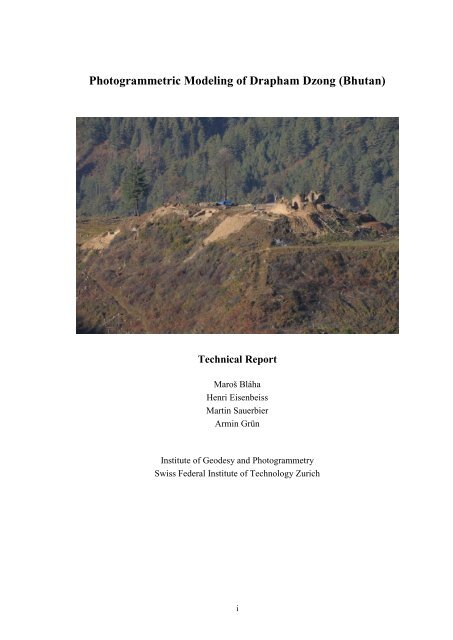
The <strong>Drapham</strong> <strong>Dzong</strong> is a ruin complex located in the District <strong>of</strong> Bumthang in central <strong>Bhutan</strong>.<br />
According to oral tradition the ancient citadel was built in 15 th /16 th century. Nowadays there is<br />
an archeological excavation at the <strong>Drapham</strong> <strong>Dzong</strong> which is part <strong>of</strong> the first archeological project<br />
in the Kingdom <strong>of</strong> <strong>Bhutan</strong>. The main wall structures <strong>of</strong> the excavation, including the solid<br />
main tower (the so-called Utze), are located on the top <strong>of</strong> an approximately 80 m high hill in the<br />
valley and cover an area <strong>of</strong> 225 m x 100 m (figure 1). These structures are surrounded by watchtowers<br />
in the corners. Further ruin objects are situated on the eastern bottom <strong>of</strong> the rocky hill<br />
(figure 2). One <strong>of</strong> those objects adjoins a nearby brook. The structures at the foot <strong>of</strong> the hill<br />
represent the reputed economic center <strong>of</strong> the castle complex whereas the object next to the<br />
brook served most probably as water mill. In addition there are two fortified staircases which<br />
connect the different parts <strong>of</strong> the ancient castle complex. The whole area <strong>of</strong> the excavation lies<br />
at an altitude <strong>of</strong> almost 2900 m a. s. l. (Grün, et al., 2010; SLSA, 2013).<br />
Figure 1: Hill with the main ruin structures <strong>of</strong> <strong>Drapham</strong> <strong>Dzong</strong>.<br />
1
Introduction<br />
Figure 2: Further ruin objects at the bottom <strong>of</strong> the hill.<br />
The Documentation <strong>of</strong> <strong>Drapham</strong> <strong>Dzong</strong><br />
The documentation <strong>of</strong> <strong>Drapham</strong> <strong>Dzong</strong> is a collective project by ETH Zurich, SLSA (Swiss-<br />
Liechtenstein Foundation <strong>of</strong> Archaeological Research Abroad) and Helvetas. Its aim is to generate<br />
a digital 3D model <strong>of</strong> the ruin which can be used for further works e.g. in archeology. The<br />
whole documentation project was carried out within the framework <strong>of</strong> the first archeological<br />
project in <strong>Bhutan</strong>.<br />
The here presented work shows the acquired data during the field campaign in <strong>Bhutan</strong> (November<br />
2009), the photogrammetric processing and the obtained results. In combination with some<br />
further works which are described in chapter 5, the results gathered in this project build the<br />
foundation <strong>of</strong> the visualizations at the exhibition ate the Rietberg Museum (Sacred art from the<br />
Himalayas, 2010).<br />
1.2 Research Goals<br />
During the field campaign from 2 - 13 November 2009, the whole ruin complex <strong>of</strong> <strong>Drapham</strong><br />
<strong>Dzong</strong> was documented with photogrammetric recording methods. Thereby the main part <strong>of</strong> the<br />
excavation, located on the top <strong>of</strong> the hill, was recorded with the mini-UAV (Unmanned Aerial<br />
Vehicle) system MD4-200 from Microdrones. The MD4-200 is an electrically powered quadrotor<br />
with a diameter <strong>of</strong> less than 70 cm and an empty weight <strong>of</strong> 585 g. These parameters allowed<br />
for its easy transportation from Switzerland to <strong>Bhutan</strong> which was one <strong>of</strong> the reasons why this<br />
UAV system was chosen for this project. A second constitutive reason was the successful flight<br />
test at the Jungfraujoch (Switzerland) with the MD4-200 (figure 3). The height test was accomplished<br />
in summer 2009 and showed that the system copes well with the little air present at a<br />
height <strong>of</strong> up to 3000 m a.s.l. (Sauerbier and Eisenbeiss, 2010).<br />
2
Introduction<br />
Figure 3: The MD4-200 during a test flight at the Jungfraujoch (Switzerland).<br />
However, the autonomous flight modus was not working during the data acquisition in <strong>Bhutan</strong>.<br />
Therefore the photographs were acquired in the GPS-based assisted flight modus. At the same<br />
time, the image overlap was controlled by the operator on the ground control station, using the<br />
live-view modus (Grün, et al., 2010). Table 1 shows the summarized parameters <strong>of</strong> the flight<br />
planning in <strong>Bhutan</strong>.<br />
Table 1: Main parameters <strong>of</strong> the flight planning in <strong>Bhutan</strong> (Sauerbier and Eisenbeiss, 2010).<br />
Area<br />
<strong>Bhutan</strong><br />
H g<br />
120 m<br />
f<br />
4.4 mm<br />
GSD<br />
4-5 cm<br />
v UAV<br />
2 m/s<br />
Flight mode<br />
Assisted<br />
Acquisition mode<br />
Cruising<br />
Size <strong>of</strong> the area<br />
350 m x 200 m<br />
p/q 75/75 %<br />
Due to technical problems with the remote control <strong>of</strong> the MD4-200 some parts <strong>of</strong> the excavation<br />
could not be recorded with aerial images. For this reason the ruin objects underneath the hill<br />
were documented with terrestrial pictures.<br />
Besides the acquisition <strong>of</strong> the image data, eleven GCPs (Ground Control Points) were surveyed<br />
during the field campaign in November 2009. These points were placed temporarily by the project<br />
team and served for the purpose <strong>of</strong> the absolute orientation in the photogrammetric processing.<br />
Seven out <strong>of</strong> the eleven GCPs covered the area with the main citadel whereas the remaining<br />
four were located at the foot <strong>of</strong> the hill. All GCPs were measured with two GNSS receivers<br />
GPS 500 from Leica Geosystems. In the process, one system was positioned as reference<br />
station while the other was used for the individual measurements <strong>of</strong> the numerous GCPs<br />
(Grün, et al., 2010).<br />
3
Introduction<br />
Figure 4: GPS 500 during measurement <strong>of</strong> a GCP.<br />
1.3 Outline<br />
The main objective was set on the reconstruction <strong>of</strong> several ruin structures. A further ambition<br />
was to generate an orthoimage <strong>of</strong> the main ruin complex situated on the hilltop. The basic principle<br />
<strong>of</strong> both procedures, the modeling as well as the orthoimage generation, is the photogrammetric<br />
processing <strong>of</strong> the image data which was acquired in <strong>Bhutan</strong>. In particular, the photogrammetric<br />
processing contains the following steps:<br />
<br />
<br />
<br />
<br />
<br />
Preprocessing <strong>of</strong> the images (UAV images and terrestrial images)<br />
Orientation <strong>of</strong> the images (UAV images and terrestrial images)<br />
DTM generation (UAV images and terrestrial images)<br />
Orthoimage generation (UAV images)<br />
Measurement <strong>of</strong> the ruin structures (terrestrial images)<br />
The raw data which was available for this project consisted mainly <strong>of</strong> the aerial images taken<br />
with the MD4-200 and the terrestrial photographs, which can be divided into two different<br />
groups. The first group consists <strong>of</strong> pictures which describe the ruin objects at the bottom <strong>of</strong> the<br />
hill with the main castle complex. The second group contains special photographs <strong>of</strong> the walls<br />
on the hilltop. These can be used for the purpose <strong>of</strong> texture mapping which is necessary in order<br />
to generate a photorealistic model <strong>of</strong> <strong>Drapham</strong> <strong>Dzong</strong>. The Panasonic DMC-FX35 was applied<br />
for the acquisition <strong>of</strong> the UAV image data. The aerial images feature a format <strong>of</strong> 3648 x 2736<br />
pixels. The terrestrial photographs were taken with the Nikon D3X and Nikon D2XS cameras.<br />
These pictures feature a maximum format <strong>of</strong> 6048 x 4032 pixels. Moreover, there are general<br />
documentation photographs available that can be applied for several purposes (e.g. presentation<br />
and poster <strong>of</strong> this project, exhibition at the Rietberg Museum, etc.). In addition to the image<br />
data, there are coordinates <strong>of</strong> eleven GCPs which were surveyed during the field campaign in<br />
<strong>Bhutan</strong> using Geographic Coordinates. The GCPs were measured with the static GNSS measurement<br />
system GPS 500 and feature an accuracy <strong>of</strong> 1 – 2 cm. Figure 5 shows the distribution <strong>of</strong><br />
the seven GCPs on the top <strong>of</strong> the hill. The remaining four GCPs lie next to the hill in the area <strong>of</strong><br />
the further ruin objects.<br />
4
Introduction<br />
Figure 5: Overview <strong>of</strong> the GCPs at the top <strong>of</strong> the hill.<br />
5
Theory<br />
2 Theory<br />
The purpose <strong>of</strong> this chapter is to explain several theoretical basics which were applied during<br />
this work. However, the theory described within this chapter is just a simplified extract <strong>of</strong> the<br />
extensive scientific literature. Nevertheless, it makes a contribution to the general understanding<br />
<strong>of</strong> the data processing which is topic <strong>of</strong> chapter 3 and 4.<br />
2.1 Mathematic Fundamentals<br />
Central Projection<br />
In order to reconstruct the shape and position <strong>of</strong> an object from photographs, it is necessary to<br />
know the geometry <strong>of</strong> the image forming system. Basically a photograph can be considered as a<br />
central projection <strong>of</strong> the recorded object. However, the central projection is just an approximation<br />
<strong>of</strong> the real world. For the purpose <strong>of</strong> high accuracy level results, it is necessary to incorporate<br />
additional sources <strong>of</strong> error which are caused by the lens system <strong>of</strong> the camera in question<br />
(Kraus, 2007; Grün, et al., 2010).<br />
Figure 6 shows a general, simplified model <strong>of</strong> the central projection. A more detailed description<br />
can be found in the book Photogrammetry – Geometry from Images and Laser Scans<br />
(Kraus, 2007). In addition, figure 6 contains couple values which are important in the context <strong>of</strong><br />
metric cameras. The left and the right part <strong>of</strong> the illustration are not related directly to each other.<br />
Figure 6: Simplified illustration <strong>of</strong> the central projection.<br />
6
Theory<br />
The principle point is the perpendicular projection <strong>of</strong> the center <strong>of</strong> perspective on the image<br />
plane. The distance between the center <strong>of</strong> perspective and the principal point is the focal length<br />
<strong>of</strong> the applied camera. This parameter depends on the camera lens and the position <strong>of</strong> the image<br />
plane. The focal length affects the scale factor <strong>of</strong> the image directly.<br />
Collinearity Equation<br />
The relationship between an object point in the object coordinate system and an image point in<br />
the image coordinate system is defined by the collinearity equation. Since this equation is described<br />
in detail in the scientific literature, it is just mentioned here briefly in words. The elements<br />
<strong>of</strong> the collinearity equation are:<br />
The coordinates <strong>of</strong> the object point in the object coordinate system<br />
The rotation matrix 1<br />
The coordinates <strong>of</strong> the center <strong>of</strong> perspective in the object coordinate system<br />
The coordinates <strong>of</strong> the image point in the image coordinate system<br />
The coordinates <strong>of</strong> the principal point in the image coordinate system<br />
The scale factor 2<br />
The collinearity equation says that for each object point one certain image point exists. Contrariwise<br />
for each image point infinitely many object points exist. Therefore it is not possible to<br />
reconstruct an object from just one image. In order to solve this problem, it is necessary that<br />
each object is visible in at least two pictures (Kraus, 2007).<br />
2.2 The Interior Orientation<br />
Constitutive for the photogrammetric processing <strong>of</strong> metric images are the values <strong>of</strong> the interior<br />
orientation <strong>of</strong> a camera. These values allow the reconstruction <strong>of</strong> the spatial bundle rays, which<br />
are required for the generation <strong>of</strong> a digital 3D model from images. The rays are defined by the<br />
center <strong>of</strong> perspective and the coordinates <strong>of</strong> points in the image coordinate system. Hence, the<br />
parameters <strong>of</strong> the interior orientation are:<br />
<br />
<br />
The focal length<br />
The coordinates <strong>of</strong> the principal point in the image coordinate system<br />
The meaning <strong>of</strong> the focal length and the coordinates <strong>of</strong> the principal point have already been<br />
explained above. In order to achieve results on a high accuracy level it is important to consider<br />
additionally the lens distortion values. The influence <strong>of</strong> these parameters can be generally described<br />
as follows: in theory an object point, the center <strong>of</strong> perspective and the corresponding<br />
image point form a spatial ray which is assumed to be a straight line. Due to radial symmetric<br />
distortion introduced by the camera lens, the ray deviates from a straight line. This effect is<br />
caused because <strong>of</strong> the changing refraction <strong>of</strong> the light rays at the objective lens. For the purpose<br />
<strong>of</strong> an accurate photogrammetric processing, the radial symmetric distortion has to be considered<br />
in the interior orientation (Photometrix, 2009). In some cases even more parameters, e.g. the<br />
decentering distortion, are determined in addition to the radial symmetric distortion.<br />
In the case <strong>of</strong> metric cameras, the parameters <strong>of</strong> the interior orientation are provided by the<br />
camera manufacturer in a calibration protocol. Contrariwise the interior orientation <strong>of</strong> <strong>of</strong>f-theshelf<br />
cameras is usually not known and has to be determined. This procedure is called camera<br />
calibration.<br />
1 The rotation matrix describes the orientation <strong>of</strong> an image in the object coordinate system.<br />
2 The scale factor is defined among others by the focal length <strong>of</strong> the concerning camera. In the case <strong>of</strong><br />
aerial images the scale factor is defined as ratio <strong>of</strong> the focal length to the flying height.<br />
7
Theory<br />
2.3 The Exterior Orientation<br />
The parameters <strong>of</strong> the exterior orientation describe the position <strong>of</strong> an image in object space.<br />
With the aid <strong>of</strong> these parameters, combined with the values <strong>of</strong> the interior orientation, it is possible<br />
to reconstruct an object in its real shape and position. Each image features six parameters<br />
<strong>of</strong> the exterior orientation:<br />
The spatial coordinates <strong>of</strong> the center <strong>of</strong> perspective in the object coordinate system<br />
The angles <strong>of</strong> rotation with respect to the axes <strong>of</strong> the object coordinate system 3<br />
There are basically two different methods for determining the parameters <strong>of</strong> the exterior orientation:<br />
the direct and the indirect georeferencing. If a GPS/IMU 4 system is used while taking the<br />
images, it is possible to measure the values <strong>of</strong> the exterior orientation directly during the recording<br />
process. Therefore this procedure is also known as direct georeferencing. Otherwise, if no<br />
GPS/IMU is available, the parameters <strong>of</strong> the exterior orientation have to be determined using<br />
control points. Since this is an indirection, this method is called indirect georeferencing (Kraus,<br />
2007).<br />
2.4 Image Orientation<br />
Image orientation is a prerequisite for the generation <strong>of</strong> 3D models from images. The purpose <strong>of</strong><br />
this procedure is to re-establish the geometrical relations <strong>of</strong> the central projection in order to be<br />
able to reconstruct an object in its real shape and position. For this re-establishment, the parameters<br />
<strong>of</strong> the interior and exterior orientation are required. The purpose <strong>of</strong> the image orientation is<br />
depicted in figure 7. Thereby the descriptions S1, S2 and S3 represent the particular centers <strong>of</strong><br />
perspective and the camera locations respectively.<br />
Figure 7: Purpose <strong>of</strong> image orientation: determination <strong>of</strong> object points on the basis <strong>of</strong> intersecting rays<br />
(Photometrix, 2009).<br />
3 For the angles <strong>of</strong> rotation <strong>of</strong>ten the identifiers ω, φ and κ are used.<br />
4 IMU stands for Inertial Measurement Unit.<br />
8
Theory<br />
There are several methods <strong>of</strong> image orientation. One <strong>of</strong>ten applied method is the block triangulation.<br />
Since this procedure was also used for the UAV image orientation, it is briefly explained<br />
below. To describe all other procedures in detail would excess the frame <strong>of</strong> this report. A circumstantial<br />
description <strong>of</strong> different orientation methods including the exact mathematical backgrounds<br />
can be found in the book Photogrammetry – Geometry from Images and Laser Scans<br />
(Kraus, 2007). However, the image orientation can be split basically into two procedures – the<br />
relative and the absolute orientation – which are explained hereafter. For the purpose <strong>of</strong> a good<br />
comprehensibility, it is assumed that only two images are oriented. Furthermore, the interior<br />
orientation is assumed to be known while the exterior orientation is computed by the way <strong>of</strong><br />
indirect georeferencing. This means that overall twelve parameters <strong>of</strong> the exterior orientation<br />
need to be determined (six for each image). It should be mentioned that in reality there are usually<br />
more than two images which are processed during image orientation.<br />
Relative Orientation<br />
In the first part <strong>of</strong> image orientation the relative position and orientation <strong>of</strong> the images are determined.<br />
This process is called relative orientation. The relative orientation is conducted by the<br />
measuring <strong>of</strong> tie points in the pictures. Tie points represent the intersection <strong>of</strong> homologous rays 5<br />
and are usually significant, static points equally distributed over the overlapping area <strong>of</strong> the two<br />
images. The result <strong>of</strong> the relative orientation is a stereo model 6 <strong>of</strong> the recorded area in the model<br />
coordinate system 7 . Though, the stereo model features an arbitrary scale, position and orientation<br />
in space. Hence it follows that it does not have any reference with a global coordinate system.<br />
The determination <strong>of</strong> these parameters is part <strong>of</strong> the absolute orientation.<br />
The mathematical basis for the relative orientation is the coplanarity condition which is defined<br />
by nine parameters. Since the relative orientation is defined by just five parameters, the remaining<br />
four parameters can be fixed arbitrarily. For that reason there are different possible methods<br />
<strong>of</strong> the relative orientation, depending on which parameters are fixed and which ones are computed.<br />
Absolute Orientation<br />
In the part <strong>of</strong> the relative orientation, five <strong>of</strong> overall twelve parameters <strong>of</strong> the exterior orientation<br />
were determined. The remaining seven parameters have to be computed in the absolute<br />
orientation process. These seven parameters describe a 3D similarity transformation which is<br />
applied on the stereo model from the relative orientation. Through this transformation the coherence<br />
between the model coordinate system and the object coordinate system accrues whereby<br />
the stereo model regains its original scale, position and orientation.<br />
As previously mentioned above, in this case the absolute orientation is carried out through control<br />
points. Control points are spots whose coordinates are known in a superior coordinate system,<br />
mostly a national coordinate system. There are three different sorts <strong>of</strong> control points:<br />
<br />
<br />
<br />
Full control point (X, Y and Z are known)<br />
Horizontal control point (X and Y are known)<br />
Height control point (Z is known)<br />
Since the 3D similarity transformation is defined by seven parameters, there are at least seven<br />
pieces <strong>of</strong> control point information required in order to accomplish an absolute orientation.<br />
Thereby four out <strong>of</strong> the seven pieces <strong>of</strong> control point information must be horizontal infor-<br />
5 Homologous rays are defined by image points <strong>of</strong> an identical object point and intersect in the corresponding<br />
point in object space.<br />
6 A stereo model in the model coordinate system is defined by all intersections <strong>of</strong> homologous rays. The<br />
precondition for such a model is the successful relative orientation <strong>of</strong> the images.<br />
7 The model coordinate system lies in an arbitrary position in space. It features no reference to a subordinate<br />
coordinate system.<br />
9
Theory<br />
mation. Therefore it follows that for an absolute orientation at least two horizontal control<br />
points and three height control points or two full control points and one height control point<br />
must be available.<br />
Block Triangulation<br />
In this procedure, the relative and absolute orientation are calculated in one step. Hereby the<br />
coherence between the image coordinates and the object coordinates is determined directly and<br />
without a loop way over the model coordinates. The unknown values <strong>of</strong> the block triangulation<br />
are the parameters <strong>of</strong> the exterior orientation. Furthermore, the object coordinates <strong>of</strong> all measured<br />
tie points also need to be determined. As observations serve the image coordinates <strong>of</strong> the<br />
control points and <strong>of</strong> the tie points. It is presumed that the coordinates <strong>of</strong> the control points are<br />
known. The adjustment principle can be described in the following way: the homologous rays<br />
are dislocated and rotated in such a way that they intersect the tie points as precisely as possible<br />
and that they converge with the control points as precisely as possible (Kraus, 2007).<br />
2.5 Digital Terrain Models<br />
A digital terrain model (DTM) describes the spatial characteristics <strong>of</strong> the topography. Thereby<br />
the spatial distribution <strong>of</strong> the terrain is usually represented by a horizontal coordinate system (X,<br />
Y) whereas the terrain characteristic is given by the corresponding Z coordinate. Moreover, a<br />
distinction can be made between 2.5D and 3D data. In the case <strong>of</strong> 2.5D data, there is exactly one<br />
corresponding Z value for each X, Y tuple. On the contrary, in 3D models it is possible that an<br />
X, Y tuple has several Z values.<br />
There are different possibilities in order to describe the topographic characteristics. Essentially<br />
the ground surface level can be described in two different ways:<br />
<br />
<br />
Models which represent the bare topography without any objects like e.g. trees or buildings.<br />
The generic term for such types <strong>of</strong> models is DTM (Digital Terrain Model).<br />
Models which describe the earth’s surface including objects like trees or buildings. These<br />
models can be generalized under the term DSM (Digital Surface Model).<br />
Figure 8 illustrates the difference between a DTM and a DSM.<br />
Figure 8: Difference between a DTM and a DSM (Hanusch, 2009).<br />
A DSM can be generated through both manual measurement as well as automatic DSM generation.<br />
In the following, the latter procedure is briefly described. The automatic DSM generation<br />
is based upon corresponding descriptions <strong>of</strong> identical objects. This process is also called matching.<br />
Relatively oriented images are a prerequisite for a successful matching. The final result is a<br />
3D point cloud. However, the spots within the point cloud are distributed irregularly which is<br />
one <strong>of</strong> the reasons why it is not appropriate for the purpose <strong>of</strong> visualization. Therefore, the point<br />
cloud is <strong>of</strong>ten processed again into a more demonstrative data model. Two representations <strong>of</strong>ten<br />
encountered are:<br />
10
Theory<br />
<br />
<br />
GRID: In this representation the spatial data is available in a regular raster. The raster follows<br />
from the interpolation 8 into the original points <strong>of</strong> the 3D point cloud.<br />
TIN (Triangulated Irregular Network): In a TIN the points <strong>of</strong> the 3D point cloud are meshed<br />
to not overlapping triangles without any gap. The benefit <strong>of</strong> a TIN compared with a GRID<br />
is that it is possible to visualize more complex surfaces.<br />
2.6 Orthoimage Generation<br />
An orthoimage corresponds to a parallel projection with a consistent scale factor in the whole<br />
image. In contrast to a common photograph, which is generally an inclined central projection, it<br />
features no <strong>of</strong>fset stacking, thus allowing reliable distance measurements. Additionally, it is<br />
possible to superpose an orthoimage on an ordinary map correctly. Typical application areas for<br />
orthoimages are e.g. photorealistic maps or visualization products in general.<br />
In order to be able to generate an orthoimage the orientation data <strong>of</strong> an image (interior and exterior)<br />
and the associated DTM are required. There are two methods <strong>of</strong> orthoimage generation: the<br />
direct and the indirect method. From a mathematical point <strong>of</strong> view, both techniques are based<br />
upon the same foundations. Since the indirect method is <strong>of</strong>ten preferred, only this will be explained<br />
in the following section. The main procedures <strong>of</strong> an indirect orthoimage generation are:<br />
<br />
<br />
<br />
<br />
Firstly, an X, Y matrix consisting <strong>of</strong> quadratic elements is spread out on the layer <strong>of</strong> the<br />
orthoimage.<br />
In the next step, the corresponding Z value for each X, Y tuple is computed using the available<br />
DTM.<br />
Afterwards, the collinearity equation is implemented as follows: the previously calculated Z<br />
value and the center <strong>of</strong> perspective <strong>of</strong> the image build a line which intersects with the image<br />
plane. This intersection defines the image point (x’, y’) which corresponds to the X, Y tuple<br />
in the orthoimage.<br />
Finally, the grey tone <strong>of</strong> the above determined image point (x’, y’) is interpolated onto the<br />
corresponding X, Y tuple in the orthoimage.<br />
Figure 9 shows the process <strong>of</strong> indirect orthoimage generation in a simplified manner. The identifiers<br />
<strong>of</strong> the indirect orthoimage generation process described above are related to those in figure<br />
9.<br />
Figure 9: Indirect method <strong>of</strong> orthoimage generation (Photogrammetrie GZ, 2009).<br />
8 The purpose <strong>of</strong> the interpolation process is to determine a closed surface by considering the original<br />
spots <strong>of</strong> the 3D point cloud. This can be accomplished in two different ways: Interpolation or Approximation.<br />
11
Processing <strong>of</strong> the UAV Images<br />
3 Processing <strong>of</strong> the UAV Images<br />
The following chapter describes all steps which were accomplished during the processing <strong>of</strong> the<br />
UAV image data. Thereby, most <strong>of</strong> the applied processes are based on the theoretical basics<br />
described in chapter 2. Furthermore, this work step can be divided into two parts: processing <strong>of</strong><br />
two image strips and processing <strong>of</strong> the overview images. Unless particularly mentioned, the<br />
procedures in both parts were identical. Three orthoimages and an overview map <strong>of</strong> the main<br />
ruin complex <strong>of</strong> <strong>Drapham</strong> <strong>Dzong</strong> resulted from the UAV image processing.<br />
3.1 Calibration <strong>of</strong> the Panasonic Lumix DMC-FX35<br />
General Information about the Panasonic Lumix DMC-FX35<br />
For the acquisition <strong>of</strong> the UAV images, the camera model Panasonic Lumix DMC-FX35 was<br />
used. The DMC-FX35 is a compact camera with a zoom lens and a maximum format <strong>of</strong><br />
3648 x 2736 pixels. As already mentioned above, the documentation images <strong>of</strong> the <strong>Drapham</strong><br />
<strong>Dzong</strong> also feature this resolution. Additional functions <strong>of</strong> the DMC-FX35 include an image<br />
stabilizer, a shutter <strong>of</strong> up to two milliseconds and a live-view video function (Sauerbier and<br />
Eisenbeiss, 2010).<br />
Computation <strong>of</strong> the Exact Pixel Size<br />
Constitutive for an accurate camera calibration is the value <strong>of</strong> the exact pixel size. In fact, a<br />
wrong pixel size can lead to satisfactory calibration results, but the calculated focal length <strong>of</strong> the<br />
concerned camera will be incorrect. As a result, a wrong pixel size causes a scaling effect<br />
(Photometrix, 2009). Since the pixel size was not provided by the camera’s manufacturer, it was<br />
necessary to calculate this value in a roundabout way using the available technical data.<br />
On the www.dpreview.com website, among others, the following technical parameters concerning<br />
the DMC-FX35 can be found:<br />
Table 2: Technical parameters <strong>of</strong> the Panasonic Lumix DMC-FX35 which were used for the computation <strong>of</strong><br />
the exact pixel size.<br />
Sensor photo detection<br />
Sensor width<br />
Sensor height<br />
10.7 megapixel<br />
6.13 mm<br />
4.6 mm<br />
Using the data in table 2 it was possible to calculate the pixel size <strong>of</strong> the Panasonic Lumix<br />
DMC-FX35. Thereby it had to be foreclosed that a pixel was generally assumed to be quadratic.<br />
The first step in this procedure was the calculation <strong>of</strong> the sensor size, which was obtained<br />
through the multiplication <strong>of</strong> the sensor width (6.13 mm) and sensor height (4.6 mm). Hence a<br />
sensor size <strong>of</strong> 28.198 mm 2 followed. In order to ascertain the size <strong>of</strong> one pixel, the<br />
28.198 mm 2 were divided by 10700000 which resulted in a pixel size <strong>of</strong> 2.6353e-6 mm 2 . The<br />
square root results to a pixel size <strong>of</strong> 1.62 microns (same for x and y direction).<br />
Calibration <strong>of</strong> the Panasonic Lumix DMC-FX35<br />
The calibration <strong>of</strong> the Panasonic DMC-FX35 was performed with the s<strong>of</strong>tware package iWitness.<br />
Via the AutoCal command, iWitness computed an automated camera calibration by using<br />
twelve color coded targets arranged in the shape <strong>of</strong> a rectangle (figure 10). Thereby two <strong>of</strong> the<br />
targets need to be elevated. The reason therefore is that the height is correlated directly with the<br />
focal length. An accurate and reliable camera calibration requires images taken from different<br />
viewpoints, rotations and distances to the object. Obviously it is necessary that the targets are<br />
12
Processing <strong>of</strong> the UAV Images<br />
visible in the recorded pictures. Since the DMC-FX35 was already stored in the iWitness database,<br />
no input values needed to be entered for an automated camera calibration. The only parameter<br />
which was saved wrongly and needed to be corrected was the above computed pixel<br />
size (1.62 microns).<br />
Figure 10: Example <strong>of</strong> a picture which was used for the calibration <strong>of</strong> the Panasonic Lumix DMC-FX35.<br />
For the calibration <strong>of</strong> the Panasonic DMC-FX35 21 photographs <strong>of</strong> the targets were taken from<br />
different positions. The results <strong>of</strong> the calibration including all significant camera parameters are<br />
listed in table 3. Furthermore, the parameters K1, K2 and K3 in table 3 represent the radial distortion<br />
<strong>of</strong> the camera lens.<br />
Table 3: Calibration results <strong>of</strong> the Panasonic Lumix DMC-FX35.<br />
Resolution, width<br />
Resolution, height<br />
Pixel width<br />
Pixel height<br />
Focal length<br />
Coordinate xp, principal point<br />
Coordinate yp, principal point<br />
K1<br />
K2<br />
K3<br />
3648 pixels<br />
2736 pixels<br />
1.6 microns<br />
1.6 microns<br />
4.3968 mm<br />
0.0078 mm<br />
0.0414 mm<br />
-1.0888e-003<br />
3.6922e-004<br />
-1.2841e-005<br />
3.2 Preprocessing <strong>of</strong> the UAV Images<br />
Image Selection<br />
Before image orientation was carried out, the UAV photographs were preprocessed. The first<br />
step in this context was the selection <strong>of</strong> appropriate images according to the criteria: image<br />
sharpness, lighting conditions, orientation and overlapping areas <strong>of</strong> the pictures. Since all fol-<br />
13
Processing <strong>of</strong> the UAV Images<br />
lowing procedures depended on this image selection, it was important for it to be completed<br />
very carefully. Thereby highest priority was placed on image sharpness and lighting conditions.<br />
Furthermore, the pictures needed to have a sufficient overlapping area <strong>of</strong> 60% or more. In order<br />
to clarify the meaning <strong>of</strong> the above mentioned criteria, the following table was created:<br />
Table 4: Criteria <strong>of</strong> the image selection.<br />
Criterion Appropriate picture(s) Inappropriate picture(s)<br />
Image sharpness<br />
Lighting Conditions<br />
Orientation<br />
Overlapping area<br />
During the field campaign in November 2009, 202 aerial images overall were taken with the<br />
MD4-200. The data content <strong>of</strong> these images is the hill with the main part <strong>of</strong> the ruin complex.<br />
The aerial photographs can be divided into three different groups. The first group contains overview<br />
images which served mainly for the purpose <strong>of</strong> the flight planning. Each one <strong>of</strong> the remaining<br />
two groups forms one image strip whereas the strips proceed parallel to each other in a<br />
northeast to southwest direction. At first all blurred and overexposed pictures were deselected.<br />
In the next step the photographs with an overlapping area <strong>of</strong> approximately 60% or more in<br />
addition to an appropriate orientation were sorted out. Thus, with regard to the photogrammetric<br />
processing and the final products, it was important that the selected images covered the whole<br />
14
Processing <strong>of</strong> the UAV Images<br />
hill including the main structures <strong>of</strong> <strong>Drapham</strong> <strong>Dzong</strong>. The result <strong>of</strong> the image selection were 6<br />
overview images and two image strips consisting <strong>of</strong> 8 and 10 images for strip one and two respectively.<br />
The following figure shows the adjustment <strong>of</strong> the two image strips which were used<br />
for the image orientation (Grün, et al., 2010). It should be mentioned that in each <strong>of</strong> the two<br />
strips an additional two pictures were deactivated because they interfered with the results <strong>of</strong> the<br />
image orientation in LPS.<br />
Image strip 1<br />
Image strip 2<br />
Figure 11: Adjustment <strong>of</strong> the selected UAV images.<br />
Image Enhancement<br />
Despite the above mentioned image selection procedure, the selected pictures still featured some<br />
shortcomings in image quality (e.g. overexposure). Therefore the second part <strong>of</strong> the preprocessing<br />
was the enhancement <strong>of</strong> the selected images, such that these shortcomings could be<br />
reduced. This step was only applied to the two image strips. It was accomplished with Adobe<br />
Photoshop and included image contrast and brightness enhancement. Since the images <strong>of</strong> the<br />
two strips were acquired on different days and day time, they featured different lighting conditions.<br />
For this reason the strips were edited individually. The exact enhancement values <strong>of</strong> Photoshop<br />
which were applied to the image strips can be extracted from the following table (Grün,<br />
et al., 2010):<br />
Table 5: Enhancement values <strong>of</strong> the UAV images in Photoshop.<br />
Contrast<br />
Brightness<br />
Strip 1 (2 nd flight) -25 -35<br />
Strip 2 (2 nd flight) -25 -35<br />
Strip 2 (3 rd flight) -15 -10<br />
Image Caption<br />
In order to simplify the following procedures, it was necessary to develop a systematic caption<br />
code for the selected images <strong>of</strong> the two image strips. This meant that each name should be significant<br />
and contain the strip number and the enhancement procedures which were applied to<br />
the picture in question. Also, the original name <strong>of</strong> the image should be present in the new caption.<br />
The outcome <strong>of</strong> these requirements was the following code, which is explained here in two<br />
examples:<br />
<br />
<br />
1B_1S_2F_P1030955_Brightness_Contrast_gedreht<br />
1B_2S_3F_P1040075_Brightness_Contrast_gedreht<br />
15
Processing <strong>of</strong> the UAV Images<br />
The letters B, S and F stand for the German words Bild (Eng. image), Streifen (Eng. strip) and<br />
Flug (Eng. flight). Hence it is possible to conclude that both examples represent the first photograph<br />
per strip, whereas the examples were taken during the second and third flight respectively.<br />
The numeration within both strips proceeds from northeast to southwest. The original name<br />
<strong>of</strong> the image as it was given by the camera then follows. Last but not least the steps which were<br />
applied to the picture during image enhancement are retained. Here the German word gedreht<br />
(Eng. rotated) informs us that the selected images were rotated 90 degrees clockwise. The rotation<br />
<strong>of</strong> the images does not affect the results <strong>of</strong> the following image orientation. However, this<br />
step helps with regard to the measurement <strong>of</strong> tie points in the photogrammetric processing with<br />
LPS (Leica Photogrammetry Suite). Since the number <strong>of</strong> the selected overview images was<br />
substantially lower than that <strong>of</strong> the image strips, it was not necessary to apply a caption code in<br />
this case.<br />
3.3 Orientation <strong>of</strong> the UAV Images<br />
The orientation <strong>of</strong> the UAV image data was accomplished with the s<strong>of</strong>tware Leica Photogrammetry<br />
Suite 9.2 (LPS). Before one was able to properly start processing the pictures some preparation<br />
work was necessary. The first step (after the LPS project had been set up and the UAV<br />
images imported) at this stage was to import the parameters <strong>of</strong> the interior orientation. Since the<br />
UAV images <strong>of</strong> the two image strips were rotated 90 degrees clockwise, it was necessary to<br />
adjust the coordinate values <strong>of</strong> the principle point. Table 6 shows the relation between the old<br />
and the new coordinates <strong>of</strong> the principal point. In the case <strong>of</strong> the overview images it was not<br />
necessary to convert the coordinates <strong>of</strong> the principal point.<br />
Table 6: Adjustment <strong>of</strong> the coordinates <strong>of</strong> the principal point (Panasonic Lumix DMC-FX35 camera).<br />
Old (iWitness)<br />
New (LPS)<br />
x-coordinate 0.0078 mm 0.0414 mm<br />
y-coordinate 0.0414 mm -0.0078 mm<br />
The remaining calibration parameters (focal length and radial distortion) were taken directly<br />
from the iWitness calibration report without any changes. The calculation <strong>of</strong> image pyramids<br />
subsequently followed. Here the resolution was modulated on three zoom levels which are used<br />
in LPS.<br />
Once all preparation work was completed, it was possible to start with the image orientation.<br />
Firstly, the coordinates <strong>of</strong> the surveyed GCPs were imported into the LPS project (in this case<br />
the GCPs represent full control points). Because these coordinates were not available in the<br />
required UTM format, they first had to be converted. This conversion was performed with the<br />
online s<strong>of</strong>tware Geographic/UTM Coordinate Converter (Taylor, 2013). It was then possible to<br />
import the coordinates <strong>of</strong> the ground control points and measure them in the LPS Classic Point<br />
Measurement Tool. In order to avoid confusion in the subsequent image processing it was important<br />
that the measured points had a systematic ID number. For this purpose the following ID<br />
code was applied:<br />
<br />
<br />
<br />
<br />
1XXX for all GCPs<br />
2XXX for all tie points within the first image strip<br />
3XXX for all tie points within the second image strip<br />
4XXX for all tie points between the first and the second image strip<br />
The next step in the image orientation - measurement <strong>of</strong> the tie points – was also carried out in<br />
the Classic Point Measurement Tool <strong>of</strong> LPS. Thereby the tie points in all overlapping areas<br />
within the image strips (i.e. the 2XXX and 3XXX points) were firstly measured. This part consisted<br />
mainly <strong>of</strong> the manual tie point measurement and the automatic tie point generation. For<br />
the purpose <strong>of</strong> a good automatic tie point generation it was important that the manually meas-<br />
16
Processing <strong>of</strong> the UAV Images<br />
ured tie points were distributed equally in the overlapping areas <strong>of</strong> the pictures. This was necessary<br />
both for the position as well as for the height. For the manually measured tie points clear<br />
spots, e.g. corners <strong>of</strong> walls, were <strong>of</strong>ten used. Figure 12 shows a typical example <strong>of</strong> a manually<br />
measured tie point in LPS. Also visible in figure 12 is the symmetric division <strong>of</strong> the screen into<br />
two halves. Each <strong>of</strong> them represents an aerial image in three different zoom levels. Related to<br />
the left image the display window in the top left corner shows the lowest zoom level whereas<br />
the window to the right shows the highest zoom level. The big image section below shows the<br />
middle zoom level <strong>of</strong> the left image.<br />
Figure 12: Example <strong>of</strong> a manually measured tie point in LPS.<br />
In this project approximately 6 points were measured manually in each overlapping area. These<br />
spots were used as initial measurements for the automated tie point generation (Grün, et al.,<br />
2010). The automated tie point generation is based on a matching procedure, whereby the coefficient<br />
limit was set at 0.95 here. By the use <strong>of</strong> such a high coefficient limit, the probability <strong>of</strong><br />
blunders is reduced. Additionally, 25 was entered as the intended number <strong>of</strong> points per image.<br />
The remaining adjustments <strong>of</strong> the automated tie point generation in LPS were kept at their default<br />
values. Despite the high coefficient limit all automatically generated tie points were controlled<br />
on blunders. In some cases LPS was not able to generate points. Forested and underexposed<br />
areas particularly featured problems in this aspect. In these areas additional tie points<br />
were measured manually. Finally, it should be mentioned that many tie points appeared in more<br />
than one overlapping area. All these points were measured in a high image ray number. This led<br />
to a more stable image block and also to better results in the image orientation.<br />
By the end <strong>of</strong> the tie point measurement all 4XXX points had been quantified. For this step the<br />
automatic tie point generation was not applied. Only a few tie points were measured in the overlapping<br />
area <strong>of</strong> the two image strips. The requests for the distribution <strong>of</strong> these points were the<br />
same as in the case <strong>of</strong> the 2XXX and 3XXX points. Finally there were ~550 (image strips) and<br />
~100 (overview images) measured tie points respectively. An overview <strong>of</strong> the measured tie<br />
points is illustrated in figure 13. The IDs <strong>of</strong> the several points have been left out as they would<br />
interfere with the clear illustration.<br />
17
Processing <strong>of</strong> the UAV Images<br />
Figure 13: Distribution <strong>of</strong> the control points and tie points in the two image strips.<br />
The next step was to calculate the block triangulation. Since in this case the working images are<br />
aerial photographs, this procedure is also called aerial triangulation. In contrast to the overview<br />
images which all were oriented in one step, the two image strips were at first oriented separately.<br />
During this process some <strong>of</strong> the photographs caused difficulties. Therefore these images<br />
were deactivated and not used for the orientation. However, this approach was only possible<br />
because the remaining photographs satisfied the requirement for a sufficient overlapping area.<br />
The images which were not used for the image orientation are:<br />
<br />
<br />
<br />
<br />
6B_1S_2F_P1030995_Brightness_Contrast_gedreht<br />
8B_1S_2F_P1040004_Brightness_Contrast_gedreht<br />
8B_2S_2F_P1040008_Brightness_Contrast_gedreht<br />
10B_2S_2F_P1040007_Brightness_Contrast_gedreht<br />
Afterwards both image strips were oriented together. Not all tie points and control points were<br />
used for the whole orientation process. The reason for this is that some points were measured<br />
imprecisely which would reduce the accuracy <strong>of</strong> the block triangulation. This especially affects<br />
the manually measured spots. Since in this project enough tie points were measured so that the<br />
mathematical model <strong>of</strong> the block triangulation was over-determined, it was possible not to use<br />
some <strong>of</strong> the redundant points for the image orientation. The following table shows the triangulation<br />
properties which were applied to the block triangulation and the results <strong>of</strong> the calculated<br />
block triangulation.<br />
18
Processing <strong>of</strong> the UAV Images<br />
Table 7: A priori triangulation properties and a posteriori triangulation summary <strong>of</strong> the two image strips.<br />
A priori triangulation properties<br />
Image point standard 0.6 pixels [x] 0.6 pixels [y]<br />
deviation (image<br />
coordinates)<br />
GCP standard deviation<br />
0.03 m [X] 0.03 m [Y] 0.03 m [Z]<br />
(object coordi-<br />
nates)<br />
A posteriori triangulation summary<br />
Total image unitweight<br />
0.5411 pixels<br />
RMSE<br />
Root mean square 0.0748 m [X] 0.0666 m [Y] 0.0828 m [Z]<br />
error <strong>of</strong> the ground<br />
coordinates<br />
Root mean square<br />
error <strong>of</strong> the image<br />
coordinates<br />
0.8126 pixels [x] 0.6570 pixels [y]<br />
An important value in the triangulation summary is the total image unit-weight RMSE; RMSE<br />
stands for Root Mean Square Error. This parameter describes the total root mean square error<br />
for the triangulation and represents the global quality <strong>of</strong> the block triangulation.<br />
3.4 DSM and Orthoimage Generation<br />
DSM Generation with SAT-PP<br />
Following the orientation <strong>of</strong> the UAV images in LPS it was possible to generate a DSM <strong>of</strong> the<br />
recorded area. In a first approach, the s<strong>of</strong>tware SAT-PP (Satellite Image Precision Processing)<br />
was applied in order to realize this step. This s<strong>of</strong>tware was developed by the Group <strong>of</strong> Photogrammetry<br />
and Remote Sensing at ETH Zurich (Zhang 2005). The main element <strong>of</strong> SAT-PP is<br />
the matching algorithm for DSM generation. Here the s<strong>of</strong>tware measures identical points in<br />
overlapping images which were taken from different positions. The basis for this process is a<br />
multi-image least-squares matching (LSM) for image features like points and edges. For the<br />
purpose <strong>of</strong> accurate and reliable results additional geometrical constraints are applied. The result<br />
is a dataset <strong>of</strong> 3D points and edges which finally are combined to a raster dataset. This dataset<br />
describes the ground surface covered by the stereo scene 9 <strong>of</strong> the images. More details concerning<br />
the above mentioned algorithm can be found in the scientific literature (Zhang, 2005; Grün,<br />
et al., 2010).<br />
In this project, a separate DSM was generated for each stereo scene but within both image strips<br />
only. In this way it was possible to extract the best parts from each DSM and combine them at<br />
the end. The result <strong>of</strong> this procedure was 5 DSMs for the first image strip and 7 DSMs for the<br />
second one. For the DSM generation the SAT-PP function Image Matching & DEM Generation<br />
for Image Stereo Pair was used. In the process Mass Points and Line Features were applied as<br />
Matching Parameters. An example <strong>of</strong> a DSM generated with the s<strong>of</strong>tware SAT-PP is illustrated<br />
in figure 14.<br />
9 A stereo scene accrues through overlapping images and allows a spatial consideration and processing <strong>of</strong><br />
the image data.<br />
19
Processing <strong>of</strong> the UAV Images<br />
Figure 14: Top-down view <strong>of</strong> a DSM generated with SAT-PP out <strong>of</strong> a stereo scene <strong>of</strong> two images. The image<br />
section shows the area around the main tower Utze.<br />
Once all DSMs were generated they were loaded into the s<strong>of</strong>tware Geomagic Studio 9. The<br />
reason for this proceeding was to choose the best parts <strong>of</strong> the particular point clouds and to<br />
combine them to one conclusive DSM which represents the recorded area. In order to avoid<br />
noise effects, caused by orientation effects, in the following interpolation it was aimed that the<br />
overlapping areas <strong>of</strong> the several models were as small as possible. On the other side it was important<br />
to avoid holes between the different DSMs. Considering these two criteria all point<br />
clouds were cropped and finally merged into a surface consisting out <strong>of</strong> 2,329,211 triangles. The<br />
merging process served mainly for the purpose <strong>of</strong> fitting the different point clouds in the overlapping<br />
areas to each other. In the end the 3D coordinates <strong>of</strong> 2,200,000 points <strong>of</strong> the merged<br />
model were exported and used for the interpolation into a GRID. This work step is described in<br />
the next paragraph.<br />
The generation <strong>of</strong> a GRID was realized with the program SCOP 5.4 (Inpho). SCOP allows to<br />
calculate a GRID with different interpolation methods. In this case two different GRID versions<br />
were generated: One with the classic prediction method and another with the robust filtering<br />
method. In both cases the GRID width was set to 0.25 m. In terms <strong>of</strong> the orthoimage generation<br />
the classic prediction conducted to an unusable result. Therefore this procedure is not exemplified<br />
here in detail anymore. Also the result <strong>of</strong> the robust filtering (figure 15) featured some<br />
shortcomings, but it was suitable for the following procedures. Some important steps <strong>of</strong> the<br />
robust filtering strategy are: Eliminate buildings, filter, interpolate, fill void areas, classify, edit,<br />
thin out and sort out. After the interpolation the GRID was loaded back into the final LPS project<br />
<strong>of</strong> the UAV images. There it was used for the calculation <strong>of</strong> an orthomosaic 10 .<br />
10 An orthomosaic is a combined picture consisting out <strong>of</strong> several orthoimages.<br />
20
Processing <strong>of</strong> the UAV Images<br />
Figure 15: GRID <strong>of</strong> <strong>Drapham</strong> <strong>Dzong</strong> area generated with SCOP 5.4.<br />
An additional DTM was measured manually by identifying corresponding points in the stereo<br />
scenes <strong>of</strong> the processed UAV images. The purpose <strong>of</strong> this proceeding was to improve the shortcomings<br />
which occurred in the automatic DSM generation. These insufficiencies induced geometrical<br />
problems in the following orthoimage rectification (see also chapter 3.5). For the manual<br />
DTM generation the stereo tool <strong>of</strong> LPS emerged as appropriate in order to measure the 3D<br />
coordinates in the <strong>Drapham</strong> <strong>Dzong</strong> ruin area (figure 16). The interpolation <strong>of</strong> these points into a<br />
GRID was carried out analogically to the automatic DSM generation. Overall, the new GRID<br />
consists <strong>of</strong> 354,144 3D points. Finally, this DTM was also used for the rectification <strong>of</strong> an additional<br />
orthoimage.<br />
Figure 16: Manually measured 3D points in the <strong>Drapham</strong> <strong>Dzong</strong> ruin area.<br />
Orthoimage Generation<br />
Based on the UAV images <strong>of</strong> the two image strips and the above calculated GRIDs two orthomosaics<br />
and an overview map <strong>of</strong> the ruin complex were produced. Furthermore, a third orthomosaic<br />
was generated based on the 6 overview images. Therefore a source DTM was used<br />
21
Processing <strong>of</strong> the UAV Images<br />
which was generated by Fabio Remondino at the Bruno Kessler Foundation in Trento (Italy).<br />
All three steps were accomplished using the LPS Mosaic Tool. Thereby the output cell size <strong>of</strong><br />
the orthoimage was set to 5 cm. The cutlines for the intersections <strong>of</strong> the images were generated<br />
automatically by means <strong>of</strong> the Automatically Generate Seamlines for Intersections function <strong>of</strong><br />
LPS. Moreover, the seams <strong>of</strong> the orthomosaic based on the manual measured DTM were edited<br />
additionally. Besides, no color corrections were applied in this process. The contrast and brightness<br />
adjustment was later carried out in Photoshop. This step was accomplished analog to the<br />
image enhancement mentioned above. The outcomes <strong>of</strong> the orthoimage generation are presented<br />
in the next chapter.<br />
3.5 Results<br />
The results <strong>of</strong> the UAV image processing are three orthomosaics and an overview map <strong>of</strong> the<br />
main ruin structures <strong>of</strong> <strong>Drapham</strong> <strong>Dzong</strong>. In the following the first image refers to the orthomosaic<br />
based on automatically generated DSM while the second one refers to the orthomosaic<br />
based on the manually measured DTM. The image source <strong>of</strong> both orthomosaics are the two<br />
strips. Finally, the third mentioned orthomosaic is based on the overview images.<br />
In its current status the first image features some shortcomings in geometry and radiometry<br />
(figure 17 and 18). While the radiometric difficulties were mainly caused by different lighting<br />
conditions in the pictures, the origin <strong>of</strong> the geometric problems is the automatically calculated<br />
DSM (see also chapter 3.4). The radiometric problems can be rectified with the LPS Color Correction<br />
functions, in addition to the general image adjustment tools in Photoshop. More problematical<br />
was the elimination <strong>of</strong> the shortcomings in the DSM. Since the ground surface <strong>of</strong> the<br />
<strong>Drapham</strong> <strong>Dzong</strong> area is very complex (it includes vegetation, walls, buildings without ro<strong>of</strong>s,<br />
holes from the excavation, etc.), it is very difficult to produce a DSM which leads to an errorfree<br />
orthoimage. One possibility in order to solve this problem is to edit the DSM manually and<br />
generate a true orthoimage based on the measured ruin structures in the digital 3D model <strong>of</strong><br />
<strong>Drapham</strong> <strong>Dzong</strong> (see also chapter 5.1). A similar approach was realized in conjunction with the<br />
second generated orthomosaic (figure 19 and 20). However, in this case a completely new DTM<br />
was measured manually instead <strong>of</strong> editing the existing DSM <strong>of</strong> the first image. The result<br />
showed a clear improvement considering the geometric and radiometric characteristics.<br />
Since the overview images have been acquired from a higher altitude (approximately 120 m)<br />
than the UAV images <strong>of</strong> the two strips, the third orthomosaic features a lower ground resolution<br />
than the first and second one (figure 21 and 22). In addition there are geometrical problems in<br />
the border areas <strong>of</strong> this image. Those are caused mainly by shortcomings in the source DTM.<br />
However, the textures in the second orthomosaic are better compared to the first two. The reason<br />
therefore are beneficial lighting conditions in the here applied aerial images.<br />
Comparing all three orthomosaics with each other one can conclude that overall the radiometric<br />
and geometrical aspects appear best in the second image. Decisive for this result are among<br />
other things the manually measured DSM in addition to the manually edited seamlines. For this<br />
reason, an overview map including contour lines and a coordinate grid was generated out <strong>of</strong> the<br />
second image (figure 23). The s<strong>of</strong>tware package which was used for this proceeding was<br />
ArcGIS.<br />
22
Processing <strong>of</strong> the UAV Images<br />
Figure 17: Orthomosaic <strong>of</strong> the area <strong>of</strong> <strong>Drapham</strong> <strong>Dzong</strong> (whole ruin complex) based on UAV images <strong>of</strong> the two<br />
image strips and the automatically generated DSM.<br />
23
Processing <strong>of</strong> the UAV Images<br />
Figure 18: Orthomosaic <strong>of</strong> the area <strong>of</strong> <strong>Drapham</strong> <strong>Dzong</strong> (main citadel) based on UAV images <strong>of</strong> the two image<br />
strips and the automatically generated DSM.<br />
24
Processing <strong>of</strong> the UAV Images<br />
Figure 19: Orthomosaic <strong>of</strong> the area <strong>of</strong> <strong>Drapham</strong> <strong>Dzong</strong> (whole ruin complex) based on UAV images <strong>of</strong> the two<br />
image strips and the manually generated DTM.<br />
25
Processing <strong>of</strong> the UAV Images<br />
Figure 20: Orthomosaic <strong>of</strong> the area <strong>of</strong> <strong>Drapham</strong> <strong>Dzong</strong> (main citadel) based on UAV images <strong>of</strong> the two image<br />
strips and the manually generated DTM.<br />
26
Processing <strong>of</strong> the UAV Images<br />
Figure 21: Orthomosaic <strong>of</strong> the area <strong>of</strong> <strong>Drapham</strong> <strong>Dzong</strong> (whole ruin complex) based on the UAV overview<br />
images.<br />
27
Processing <strong>of</strong> the UAV Images<br />
Figure 22: Orthomosaic <strong>of</strong> the area <strong>of</strong> <strong>Drapham</strong> <strong>Dzong</strong> (main citadel) based on the UAV overview images.<br />
28
Processing <strong>of</strong> the UAV Images<br />
Figure 23: Overview map <strong>of</strong> the <strong>Drapham</strong> <strong>Dzong</strong> ruin area based on the second orthomosaic.<br />
29
Processing <strong>of</strong> the Terrestrial Images<br />
4 Processing <strong>of</strong> the Terrestrial Images<br />
The topic <strong>of</strong> chapter 4 is the processing <strong>of</strong> the terrestrial images. Most procedures described<br />
hereafter were done for the same purpose as in the case <strong>of</strong> the UAV images. The theoretical<br />
backgrounds and details in context with the here mentioned methods can be found in chapter 2<br />
and 3. The result <strong>of</strong> the terrestrial image processing was a digital 3D model <strong>of</strong> two ruin objects<br />
situated at the foot <strong>of</strong> the hill with the main ruin.<br />
4.1 Calibration <strong>of</strong> the Nikon D3X<br />
General Information About the Nikon D3X<br />
For the documentation <strong>of</strong> the putative economic center <strong>of</strong> <strong>Drapham</strong> <strong>Dzong</strong> located on the eastern<br />
foot hill the Nikon D2XS and D3X camera models were used. Since the images <strong>of</strong> the<br />
D2XS were not used for the processing <strong>of</strong> the terrestrial images this camera is not mentioned in<br />
detail here. The Nikon D3X is a high-resolution reflex camera (SLR) with a maximum format<br />
<strong>of</strong> 6048 x 4032 pixels which was also applied to the terrestrial photographs <strong>of</strong> <strong>Drapham</strong> <strong>Dzong</strong>.<br />
It is possible to use the Nikon D3X in combination with a GPS receiver which allows to measure<br />
the position from which the pictures were taken. In addition the exchangeability <strong>of</strong> the<br />
lenses increases the flexibility <strong>of</strong> the camera and allows the Nikon D3X to be optimally applied<br />
in different situations.<br />
Computation <strong>of</strong> the Exact Pixel Size<br />
The exact pixel size <strong>of</strong> the Nikon D3X was computed in a different manner to that <strong>of</strong> the DMC-<br />
FX35. Additionally, in the terrestrial case the source <strong>of</strong> the required technical parameters was<br />
the webpage www.dpreview.com, and this information is also confirmed by other sources. The<br />
values which were used for the determination <strong>of</strong> the Nikon D3X pixel size are listed in table 8.<br />
Table 8: Technical parameters <strong>of</strong> the Nikon D3X which were used for the computation <strong>of</strong> the exact pixel size.<br />
Maximal format<br />
Sensor width<br />
Sensor height<br />
6048 x 4032 pixels<br />
35.9 mm<br />
24 mm<br />
The exact pixel size <strong>of</strong> the Nikon D3X was computed as follows:<br />
Firstly, the sensor width (35.9 mm) was divided by the according number <strong>of</strong> pixels (6048).<br />
Hence this resulted in a pixel side length <strong>of</strong> 5.94 microns.<br />
Secondly, the analogue calculation was performed for the sensor height (24 mm) with its<br />
corresponding number <strong>of</strong> pixels (4032). The result was a pixel side length <strong>of</strong><br />
5.95 microns which affirms the result obtained above. Additionally, this fact confirms the<br />
general assumption <strong>of</strong> quadratic pixels in chapter 3.1.<br />
Calibration <strong>of</strong> the Nikon D3X<br />
Similar to the Panasonic Lumix DMC-FX35, the Nikon D3X was also calibrated using the<br />
iWitness program. Since this process is analogous to the calibration <strong>of</strong> the DMC-FX35, it is not<br />
explained here in any more detail. However, one constitutive difference was that a separate calibration<br />
was carried out for each lens which was used on the Nikon D3X in <strong>Bhutan</strong>. Due to the<br />
fact that only the 50 mm lens was used for the terrestrial documentation <strong>of</strong> <strong>Drapham</strong> <strong>Dzong</strong>,<br />
only the results <strong>of</strong> this calibration process are shown here (table 9). The other lenses were only<br />
used for documentary pictures <strong>of</strong> the field campaign.<br />
30
Processing <strong>of</strong> the Terrestrial Images<br />
Table 9: Calibration results <strong>of</strong> the Nikon D3X.<br />
Resolution, width<br />
6048 pixels<br />
Resolution, height<br />
4032 pixels<br />
Pixel width<br />
5.9 microns<br />
Pixel height<br />
5.9 microns<br />
Focal length<br />
52.4558 mm<br />
Coordinate xp, principal point<br />
0.0949 mm<br />
Coordinate yp, principal point<br />
-0.1822 mm<br />
K1<br />
5.2256e-005<br />
K2 -1.1876-008<br />
K3<br />
-1.1761e-011<br />
4.2 Preprocessing <strong>of</strong> the Terrestrial Images<br />
Since most <strong>of</strong> the work steps during the preprocessing <strong>of</strong> the terrestrial images were very similar<br />
to the steps <strong>of</strong> chapter 3.2 only the relevant facts and results are detained in the following.<br />
Image Selection<br />
During the terrestrial documentation <strong>of</strong> <strong>Drapham</strong> <strong>Dzong</strong> all in all 95 photographs were taken.<br />
As already mentioned in the introduction the data content <strong>of</strong> these images is the eastern part <strong>of</strong><br />
the castle complex which is located at the bottom <strong>of</strong> the hill with the main ruin. This part <strong>of</strong> the<br />
excavation mainly consists <strong>of</strong> two ruin objects. The first is situated more to the west, directly<br />
next to the hill, and is slightly larger (figure 24). The smaller object represents the putative water<br />
mill <strong>of</strong> <strong>Drapham</strong> <strong>Dzong</strong> and lies more downhill (figure 25). Due to difficult topography on<br />
the site, the terrestrial photographs feature irregular recording positions. This issue complicates<br />
additionally the starting position for the data processing.<br />
Figure 24: Larger object <strong>of</strong> the additional ruin structures <strong>of</strong> <strong>Drapham</strong> <strong>Dzong</strong>.<br />
31
Processing <strong>of</strong> the Terrestrial Images<br />
Figure 25: Putative water mill <strong>of</strong> <strong>Drapham</strong> <strong>Dzong</strong>.<br />
Due to the fact that the two objects mentioned above are spread widely apart and therefore the<br />
relevant images do not feature appropriate overlapping areas, it was decided to evaluate them<br />
separately. This fact fundamentally affected the terrestrial image selection. The final images<br />
which were selected for the photogrammetric processing can be divided into two groups. The<br />
first group describes the larger object closer to the hill and consists out <strong>of</strong> 14 pictures. This<br />
group can be additionally divided into four image strips whereupon each strip shows the building<br />
from different perspectives. The data content <strong>of</strong> the second group is the smaller object. This<br />
group contains seven images and cannot be divided into any further image strips (Grün, et al.,<br />
2010). Figure 26 and 27 show the camera positions and the images which were finally used for<br />
the terrestrial image processing.<br />
Figure 26: Camera positions and the corresponding photographs <strong>of</strong> the first terrestrial image group.<br />
32
Processing <strong>of</strong> the Terrestrial Images<br />
Figure 27: Camera positions and the corresponding photographs <strong>of</strong> the second terrestrial image group.<br />
Image Enhancement<br />
The image enhancement <strong>of</strong> the terrestrial photographs was performed using Photoshop. The<br />
enhancement values which were applied to the terrestrial images are listed in table 10.<br />
Table 10: Enhancement values (in Photoshop) <strong>of</strong> the terrestrial images.<br />
Contrast<br />
Brightness<br />
Strip 1 -25 -30<br />
Strip 2 -30 -35<br />
Strip 3 -25 -30<br />
Strip 4 -25 -30<br />
Caption <strong>of</strong> the Images<br />
The caption code for the terrestrial images is essentially the same as the one <strong>of</strong> the UAV images.<br />
The only two differences are:<br />
<br />
<br />
The names <strong>of</strong> the images logically do not feature any flight number.<br />
Since the terrestrial pictures were not rotated, only the brightness and contrast are listed as<br />
enhancement values.<br />
4.3 Orientation <strong>of</strong> the Terrestrial Images<br />
For the orientation <strong>of</strong> the terrestrial images, PhotoModeler 6 emerged as a convenient s<strong>of</strong>tware.<br />
The image orientation procedure in PhotoModeler was similar to the one in LPS. However,<br />
there were some essential differences, <strong>of</strong> which the most significant was that PhotoModeler<br />
calculates the relative and the absolute orientation separately. Furthermore, as previously mentioned<br />
above the terrestrial images were processed in two groups. For this reason two separate<br />
projects were set up in PhotoModeler. In the following paragraphs, unless specifically mentioned,<br />
all procedures in the two projects were identical.<br />
The first step <strong>of</strong> the image processing in PhotoModeler was the import <strong>of</strong> the terrestrial images.<br />
Accordingly, the camera which was used to take the photographs had to be defined. Therefore<br />
the calibration values from iWitness were transferred into the project in PhotoModeler. With the<br />
33
Processing <strong>of</strong> the Terrestrial Images<br />
exception <strong>of</strong> the principal point coordinates, all values were imported without any changes. The<br />
reason why the coordinates <strong>of</strong> the principle point needed to be adjusted manually was a different<br />
definition <strong>of</strong> the point <strong>of</strong> origin <strong>of</strong> the image coordinate system. While iWitness defines this<br />
point to be in the middle <strong>of</strong> an image, PhotoModeler considers the top left <strong>of</strong> a picture as the<br />
point <strong>of</strong> origin. The relation between the old and new coordinates <strong>of</strong> the principal point is shown<br />
in table 11.<br />
Table 11: Adjustment <strong>of</strong> the principal point’s coordinates (Nikon D3X camera).<br />
Old (iWitness)<br />
New (PhotoModeler)<br />
x-coordinate 0.0949 mm 18.0949<br />
y-coordinate -0.1822 mm 12.1822<br />
The next procedure was the manual measurement <strong>of</strong> tie points in the first two images. As in the<br />
UAV photographs, a good distribution <strong>of</strong> tie points in the overlapping area was also aimed for.<br />
This procedure was accomplished with PhotoModeler’s Mark Points Mode and Referencing<br />
Mode and also included the measuring <strong>of</strong> GCPs as tie points. Since the program numbers all<br />
measured points consecutively, it was not possible to apply a systematic point code here. In<br />
general the manual measuring <strong>of</strong> tie points in the terrestrial images was more difficult than in<br />
the UAV images. As there were not as many walls as on the top <strong>of</strong> the hill, stones and stumps<br />
were also used as tie points. Figure 28 shows a typical example <strong>of</strong> a manually measured tie<br />
point in PhotoModeler.<br />
Figure 28: Example <strong>of</strong> a manually measured tie point in PhotoModeler.<br />
Furthermore, it was not possible to generate enough well distributed tie points automatically in<br />
the terrestrial images. The reason for this were occlusions and the vegetation in the overlapping<br />
areas which caused significant differences in image texture. Figure 29 shows an example <strong>of</strong><br />
automatic generated tie points in two images. Those were computed with the s<strong>of</strong>tware Gummireifen<br />
by David Novák. It is apparent that this point distribution is suboptimal. In the end,<br />
approximately 20 tie points resulted out <strong>of</strong> the manual measurement (Grün, et al., 2010).<br />
34
Processing <strong>of</strong> the Terrestrial Images<br />
Figure 29: Automatically generated tie points in two terrestrial images.<br />
After all tie points in the overlapping area were measured, the image pair was oriented relatively<br />
with the PhotoModeler Process function. In this procedure the remaining images without any tie<br />
points thus far were ignored and not oriented. After a successful orientation <strong>of</strong> the first two images<br />
both pictures were retained. This means that they were used for the following process, but<br />
the adjustment 11 <strong>of</strong> the images calculated above was not changed anymore.<br />
Now the third image was attached to the first two images and the manual measurement <strong>of</strong> tie<br />
points started from the beginning. Firstly all previously measured tie points which were visible<br />
in the new overlapping areas 12 were imported. Then some additional tie points were measured<br />
until approximately 20 well-distributed tie points were available in the new overlapping areas.<br />
11 The adjustment <strong>of</strong> the images means their relative orientation.<br />
12 One overlapping area accrues between the first and the third image and one overlapping area accrues<br />
between the second and the third image.<br />
35
Processing <strong>of</strong> the Terrestrial Images<br />
Subsequently the third image was relatively oriented with respect to the already existing adjustment<br />
<strong>of</strong> the first two images. Likewise, after processing, the image was also retained and not<br />
adjusted in the following procedures anymore. This sequence was completed for all terrestrial<br />
images. Sometimes PhotoModeler was not able to calculate a relative image orientation. This<br />
was the case if the camera positions from which the photographs were taken were too close to<br />
each other and therefore built a short base. Since this problem reoccurred several times during<br />
the processing <strong>of</strong> the terrestrial images, further photographs were sifted out and not used in the<br />
orientation process. More details in context with the number <strong>of</strong> oriented pictures are listed in<br />
table 12.<br />
Finally, the absolute orientation <strong>of</strong> the terrestrial photographs was calculated. For this procedure<br />
the previously calculated UTM coordinates <strong>of</strong> the available GCPs were used. The absolute orientation<br />
was the only step in the image orientation which was fundamentally different for the<br />
two image groups. As four GCPs were visible in the pictures <strong>of</strong> the first group, it was possible<br />
to calculate the absolute orientation <strong>of</strong> those photographs directly. Thereby the coordinates <strong>of</strong><br />
the GCPs were imported into the PhotoModeler project by using the s<strong>of</strong>tware’s Imports Explorer.<br />
The coordinates <strong>of</strong> the control points were then allocated to the corresponding points in the<br />
PhotoModeler project, which so far served as tie points. Finally a new orientation run was accomplished<br />
in which the absolute orientation <strong>of</strong> the whole image block was determined. Due to<br />
the fact that no GCPs were visible in the pictures <strong>of</strong> the second image group, it was not possible<br />
to calculate directly an absolute orientation. Therefore the absolute orientation <strong>of</strong> the second<br />
image group was calculated in a roundabout way via eccentric control points. Eccentric control<br />
points are points, whose coordinates can be computed by using already oriented images. As<br />
parts <strong>of</strong> the smaller objects were also visible in the first image group, it was possible to calculate<br />
four eccentric control points. These points enabled the absolute orientation <strong>of</strong> the second image<br />
block. The correct absolute orientation <strong>of</strong> the first image group was the precondition for this<br />
procedure (Grün, et al., 2010). The quality <strong>of</strong> the final orientation results is shown in table 12.<br />
Table 12: Results <strong>of</strong> the image orientation <strong>of</strong> the terrestrial images.<br />
Image block 1 Image block 2<br />
Total image number 12 5<br />
Oriented images 8 5<br />
Overall RMS 0.78 pixels 0.529 pixels<br />
Maximum RMS 1.483 pixels 0.922 pixels<br />
Minimum RMS 0.001 pixels 0.012 pixels<br />
Maximum point tightness 0.064 m 0.0095 m<br />
Minimum point tightness 2.5e-005 m 0.0001 m<br />
Overall RMS vector length 0.0828 m 0.0238 m<br />
Maximum vector length 0.324 m 0.044 m<br />
Minimum vector length 0.0302 m 0.0132 m<br />
4.4 <strong>Modeling</strong> <strong>of</strong> the Recorded Area<br />
The first part <strong>of</strong> the modeling was accomplished in PhotoModeler 6 likewise. Therefore the<br />
final PhotoModeler file <strong>of</strong> the image orientation was split into three different projects. In the<br />
first one, points along the top edges <strong>of</strong> all walls were measured clockwise (figure 30). This proceeding<br />
was necessary with a view to the following modeling process in CCModeler 5.0. In<br />
order to get 3D coordinates <strong>of</strong> the measured spots, all points needed to be measured in at least<br />
two images. Since some walls were obscured by trees, it was not possible to detect all structures<br />
in very high detail.<br />
36
Processing <strong>of</strong> the Terrestrial Images<br />
Figure 30: Points measured in a clockwise sense on the top edge <strong>of</strong> a ruin wall.<br />
In the second and third project <strong>of</strong> PhotoModeler further points on the bare ground were measured.<br />
In general it was aimed to measure spots in a raster pattern with a raster width <strong>of</strong> approximately<br />
1.5 m. Because <strong>of</strong> the dense vegetation on-site it was not possible to measure such points<br />
in each part <strong>of</strong> the recorded area. The spots measured in the second and third project represented<br />
the environment <strong>of</strong> the ruin structures and needed to be measured in at least two images as well.<br />
The third project in particular contained points along the bottom edges <strong>of</strong> the ruin walls. From<br />
all these points a DTM was generated by Martin Sauerbier using the s<strong>of</strong>tware DTMZ which is<br />
an interpolation program based on the finite element interpolation. Since the DTM <strong>of</strong> the smaller<br />
ruin object did not cover the whole area with all ruin walls, some additional pseudo points<br />
were inserted manually into the concerning model.<br />
The second part <strong>of</strong> the modeling was the reconstruction <strong>of</strong> the whole 3D scene with the program<br />
CCModeler 5.0. Therefore the points <strong>of</strong> the first project and the previously computed DTM<br />
were imported into a new CCModeler file. For the reconstruction <strong>of</strong> the ruin structures the<br />
House reconstruction tool <strong>of</strong> the s<strong>of</strong>tware was used. This procedure can be described in the<br />
following way: The points <strong>of</strong> the top wall edges were connected to a triangulated irregular network<br />
(TIN) which represents the upper surface <strong>of</strong> a ruin wall. The border <strong>of</strong> this surface was<br />
extruded vertically and intersected with the DTM. From this followed a water-pro<strong>of</strong> 3D model<br />
<strong>of</strong> a ruin wall (Grün, et al., 2010). This process was applied repetitively to all walls. The result<br />
was a 3D model <strong>of</strong> the whole scene.<br />
After the reconstruction some walls featured deficits in geometry. To rectify these shortcomings<br />
these walls were edited using the s<strong>of</strong>tware CC Edit 5.0. The tool which was applied in this connection<br />
was the Snap to 3D point function. Due to problems caused by the s<strong>of</strong>tware, this work<br />
step was only applied to the model <strong>of</strong> the larger ruin object closer to the hill.<br />
4.5 Results<br />
The results <strong>of</strong> the terrestrial image processing are two 3D models <strong>of</strong> the ruin objects situated on<br />
the bottom <strong>of</strong> the hill (figure 31 and 32). In the current status only the model <strong>of</strong> the larger object<br />
(figure 31) is edited. The next step in a future work should be the editing <strong>of</strong> the second model.<br />
In particular that means to straighten certain walls and to eliminate blunders which followed<br />
from the modeling process. Moreover, in the terrestrial case there are no usable texture images<br />
available. The reason for it is the difficult topography on location in addition to fences which<br />
37
Processing <strong>of</strong> the Terrestrial Images<br />
are placed directly in front <strong>of</strong> certain walls. Anyhow it was tried to furnish the model <strong>of</strong> the<br />
larger ruin object with textures. This step was done with the aid <strong>of</strong> Fabio Remondino by using<br />
the s<strong>of</strong>tware TextureMapping3D. As expected, the resulting 3D model was unusable for the<br />
purpose <strong>of</strong> the visualization. Therefore, it was not used in the further procedures. An alternative<br />
solution for this problem is to use artificial textures. Also conceivable is to extract some usable<br />
textures from the available image data and to stitch them repetitively on the digital 3D model. In<br />
order to compare different s<strong>of</strong>tware packages on their modeling capabilities, it would be also<br />
interesting to reconstruct the ruin objects with another program (e.g. a CAD s<strong>of</strong>tware).<br />
Figure 31: 3D model <strong>of</strong> the bigger ruin building resulting from the terrestrial image processing.<br />
Figure 32: 3D model <strong>of</strong> the smaller ruin building resulting from the terrestrial image processing.<br />
38
Further Works<br />
5 Further Works<br />
The work which is mentioned in this chapter was mainly done for the purpose <strong>of</strong> the visualization<br />
<strong>of</strong> <strong>Drapham</strong> <strong>Dzong</strong> at the <strong>Bhutan</strong> exhibition at the Rietberg Museum in 2010. As already<br />
mentioned in the introduction, one part <strong>of</strong> the visualization is a flyover <strong>of</strong> the larger surrounding<br />
area <strong>of</strong> <strong>Drapham</strong> <strong>Dzong</strong>. The flyover implements both, a digital model <strong>of</strong> the ruin structures as<br />
well as a rough DSM <strong>of</strong> the surrounding area <strong>of</strong> the excavation. In order to be able to generate<br />
such a DSM the required image data was needed. Therefore, a stereo scene <strong>of</strong> the adequate area<br />
was acquired at the beginning <strong>of</strong> 2010. A brief description <strong>of</strong> the DSM generation can be found<br />
in chapter 5.2. The digital model <strong>of</strong> the ruin structures consists mainly <strong>of</strong> two parts: the model<br />
<strong>of</strong> the main castle complex on the hilltop and the ruin objects downhill which were recorded<br />
with terrestrial photographs. The modeling process <strong>of</strong> the main citadel is the topic <strong>of</strong> the following<br />
chapter. The ruin objects further downhill were modeled within the bounds <strong>of</strong> the bachelor’s<br />
thesis <strong>of</strong> Maroš Bláha. This procedure is described in chapter 4 <strong>of</strong> this report. A further paragraph<br />
<strong>of</strong> this chapter shows a site map which serves also for the purpose to visualize the whole<br />
castle complex.<br />
5.1 Digital Model <strong>of</strong> the Main Ruin Structures <strong>of</strong> <strong>Drapham</strong> <strong>Dzong</strong><br />
The main ruin complex was modeled by Fabio Remondino at the Bruno Kessler Foundation in<br />
Trento (Italy). This modeling process was realized with the s<strong>of</strong>tware 3D Studio Max. A snapshot<br />
<strong>of</strong> the final result is shown in figure 33.<br />
Figure 33: 3D model <strong>of</strong> the main ruin structures <strong>of</strong> <strong>Drapham</strong> <strong>Dzong</strong>.<br />
In its current status the model features some shortcomings in both, geometry and texture mapping.<br />
However, for the production <strong>of</strong> the flyover it is possible to avoid these through the choice<br />
<strong>of</strong> a clever flight path. Indeed, for the purpose <strong>of</strong> an accurate 3D model <strong>of</strong> <strong>Drapham</strong> <strong>Dzong</strong> it is<br />
aimed to correct these insufficiencies. As an alternative to the 3D model it is also conceivable to<br />
use a DSM overlaid with an orthoimage <strong>of</strong> the concerning area for production <strong>of</strong> the flyover.<br />
5.2 Larger Area DSM and Orthoimage<br />
In order to be able to visualize a larger surrounding area <strong>of</strong> <strong>Drapham</strong> <strong>Dzong</strong> a GeoEye-1 stereo<br />
scene was acquired in January 2010. Hence a DSM with a covering area <strong>of</strong> 10.7 x 10.7 km 2 was<br />
generated by Martin Sauerbier at ETH Zurich. For this procedure the SAT-PP s<strong>of</strong>tware was<br />
39
Further Works<br />
used. The functionality and applied methods <strong>of</strong> SAT-PP are already described in chapter 3.4 <strong>of</strong><br />
this report. Furthermore, it should be mentioned that the orientation <strong>of</strong> the stereo scene was<br />
available through Rational Polynomial Coefficients (RPC); these were supplied with the images<br />
by the German Aerospace Center (DLR). Based on the generated DSM, an orthoimage was<br />
produced using the PAN channel with a ground resolution <strong>of</strong> 0.41 m and the RGB channels<br />
(1.61 m resolution) <strong>of</strong> the GeoEye-1 stereo scene. The result was a virtual textured 3D model <strong>of</strong><br />
the landscape which can be used for the flyover. Figure 34 shows an extract <strong>of</strong> the DSM generated<br />
by GeoEye-1 imagery (Grün, et al., 2010).<br />
Figure 34: View towards south on the surrounding area <strong>of</strong> <strong>Drapham</strong> <strong>Dzong</strong>. The arrow points on the ruin <strong>of</strong><br />
the castle (Grün, et al., 2010).<br />
5.3 Site Map<br />
In addition to the two above described visualization products, a map <strong>of</strong> the archaeological site<br />
was produced by Peter Fux (figure 35). The numerous wall structures on the top <strong>of</strong> the hill were<br />
measured in the LPS Stereo Analyst. The final LPS project which resulted from the UAV image<br />
orientation was used for these measurements. The visualization <strong>of</strong> the site map was produced<br />
using the ArcGIS s<strong>of</strong>tware package. This included also implementing the models <strong>of</strong> the ruin<br />
objects at the foot <strong>of</strong> the hill into the map (green area in figure 35).<br />
40
Further Works<br />
Figure 35: Map <strong>of</strong> the archaeological site at <strong>Drapham</strong> <strong>Dzong</strong> (Grün, et al., 2010).<br />
41
Conclusions<br />
6 Conclusions<br />
Based on the raw data which was acquired during the field campaign in November 2009, the<br />
photogrammetric visualization <strong>of</strong> the ruin <strong>of</strong> <strong>Drapham</strong> <strong>Dzong</strong> was accomplished within the<br />
framework <strong>of</strong> this project. Since the main citadel was recorded with aerial images while additional<br />
ruin objects were documented with terrestrial images, the starting position <strong>of</strong> the data<br />
processing was tricky. In order to achieve optimal results different photogrammetric methods<br />
and s<strong>of</strong>tware packages were applied. Furthermore the UAV images and the terrestrial images<br />
were processed separately. One <strong>of</strong> the main difficulties in the UAV image processing was the<br />
DSM generation. Because <strong>of</strong> the complex ground level <strong>of</strong> <strong>Drapham</strong> <strong>Dzong</strong> area it was not possible<br />
to generate a faultless DSM. Therefore, an additional DTM was measured manually and<br />
used for the corresponding working steps. Also the processing <strong>of</strong> the terrestrial images included<br />
problems. In this procedure, the photographs itself were the biggest challenge. Due to difficult<br />
environmental conditions on site some <strong>of</strong> the images feature occlusions and adverse perspectives.<br />
The final results <strong>of</strong> this project are three orthoimages <strong>of</strong> the main castle complex and a<br />
digital 3D model <strong>of</strong> further ruin objects adjacent to the main citadel. Products which occurred in<br />
an expanded frame <strong>of</strong> this venture are a map <strong>of</strong> the archeological site, a digital model <strong>of</strong> the<br />
main ruin structures and a larger area DSM in addition to a further orthoimage. Moreover, the<br />
modeling <strong>of</strong> the main fortress was further continued. The outcomes <strong>of</strong> this proceeding were<br />
presented on the ISPRS congress 2012 in Melbourne (Grün, et al., 2012).<br />
In spite <strong>of</strong> the above mentioned difficulties during the data processing the achieved results have<br />
potential and can be used for further works and projects e.g. in archeology. In particular, the<br />
orthoimages are appropriate for the generation <strong>of</strong> a site map. Furthermore it is possible to continue<br />
processing the present results. Especially some parts <strong>of</strong> the digital 3D model but also the<br />
orthoimages feature shortcomings which can be rectified. Moreover, it is possible to generate<br />
new products from the raw data (e.g. a physical 3D model <strong>of</strong> the <strong>Drapham</strong> <strong>Dzong</strong> ruin complex).<br />
A couple <strong>of</strong> such products have already been realized. The results <strong>of</strong> these works are<br />
shown in chapter 5.<br />
42
Bibliography<br />
Bibliography<br />
Digital Photography Review, 2013. Digital Photography Review corporate website,<br />
http://www.dpreview.com/, (accessed 29 January 2013).<br />
Eisenbeiss, H., 2009. UAV Photogrammetry, DISS. ETH NO. 18515, <strong>Institute</strong> <strong>of</strong> Geodesy and<br />
Photogrammetry, ETH Zurich, Zurich, Switzerland, p. 235.<br />
Eisenbeiss, H., Sauerbier, M., 2011. Investigation <strong>of</strong> UAV systems and flight modes for photogrammetric<br />
applications, The <strong>Photogrammetric</strong> Record 26 (136): 400-421 (December 2011),<br />
doi: 10.1111/j.1477-9730.2011.00657x.<br />
Gruen, A., Eisenbeiss, H., Blaha, M., Sauerbier, M., Fux, P., 2010. UAV Photogrammetry<br />
Project <strong>Drapham</strong> <strong>Dzong</strong>, <strong>Bhutan</strong>, SLSA-Jahresbericht 2009, SLSA, Zurich Switzerland, p. 61-<br />
70.<br />
Gruen, A., Zhang, Z., Eisenbeiss, H., 2012. UAV photogrammetry in remote areas – 3D modeling<br />
<strong>of</strong> <strong>Drapham</strong> <strong>Dzong</strong> <strong>Bhutan</strong>, In: ISPRS Archives XXXIX-B1, 2012 XXII ISPRS Congress,<br />
25 August – 01 September 2012, Melbourne, Australia.<br />
Hanusch, T., 2009. Digitale Terrainmodelle, lecture documents, digitale Photogrammetrie HS<br />
2009, <strong>Institute</strong> <strong>of</strong> Geodesy and Photogrammetry, ETH Zurich, Zurich, Switzerland, p.25.<br />
Kraus, K., 2007. Photogrammetry - Geometry from Images and Laser Scans, Walter de<br />
Gruyter, Goettingen, Germany, p.459.<br />
Meyer, W., Fischer, E., Britschgi, J., 2007. The <strong>Bhutan</strong>-Swiss Archaeological Project – The<br />
Fortification <strong>Drapham</strong> <strong>Dzong</strong> in Central <strong>Bhutan</strong>, SLSA-Jahresbericht 2007, SLSA, Zurich<br />
Switzerland, p. 29-42.<br />
Microdrones, 2010. Microdrones GmbH corporate website,<br />
http://www.microdrones.com/en_home.php, (accessed 2 May 2010).<br />
Photogrammetrie GZ, 2009. Orthophoto, lecture documents, Photogrammetrie GZ FS 2009,<br />
<strong>Institute</strong> <strong>of</strong> Geodesy and Photogrammetry, ETH Zurich, Zurich, Switzerland, p.19.<br />
Photometrix, 2009. Users Manual for iWitness and iWitnessPro, p.127.<br />
Sauerbier, M., Eisenbeiss, H., 2010. UAVs for the documentation <strong>of</strong> archaeological excavations.<br />
International Archives <strong>of</strong> Photogrammetry, Remote Sensing and Spatial Information Sciences,<br />
Vol. XXXVIII, Part 5, Commission V Symposium, Newcastle upon Tyne, UK.<br />
Schweizer Fernsehen, 2013. Achriv Übersicht 2010, Schweiz aktuell corporate website,<br />
http://videoportal.sf.tv/video?id=b9f385cc-9fe8-41ff-a588-<br />
fa470423fa61&referrer=http%3A%2F%2Fwww.sf.tv%2Fsendungen%2Fschweizaktuell%2Find<br />
ex.php%3Fdocid%3D20100409, (accessed 29 January 2013).<br />
SLSA, 2013. SLSA corporate website, http://www.slsa.ch/Projekte/<strong>Drapham</strong><strong>Dzong</strong>E.htm,<br />
(accessed 29 January 2013).<br />
Taylor, C., 2013. Geographic/UTM Coordinate Converter corporate website,<br />
http://home.hiwaay.net/~taylorc/toolbox/geography/geoutm.html, (accessed 29 January 2013).<br />
Zhang, L., 2005. Automatic digital surface model (DSM) generation from linear array images,<br />
DISS. ETH NO. 16078, <strong>Institute</strong> <strong>of</strong> Geodesy and Photogrammetry, ETH Zurich, Zurich, Switzerland,<br />
p. 219.<br />
43