Diffusion MRI: From Quantitative Measurement to In vivo ...
Diffusion MRI: From Quantitative Measurement to In vivo ...
Diffusion MRI: From Quantitative Measurement to In vivo ...

Create successful ePaper yourself
Turn your PDF publications into a flip-book with our unique Google optimized e-Paper software.
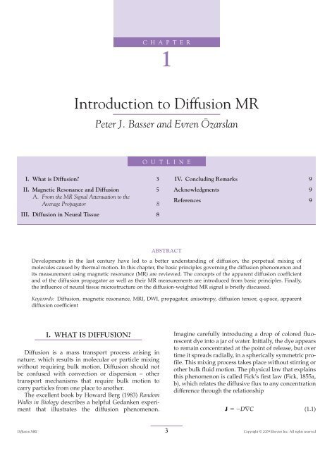
C H A P T E R<br />
1<br />
<strong>In</strong>troduction <strong>to</strong> <strong>Diffusion</strong> MR<br />
Peter J. Basser and Evren Ö zarslan<br />
O U T L I N E<br />
I. What is <strong>Diffusion</strong>? 3<br />
II. Magnetic Resonance and <strong>Diffusion</strong> 5<br />
A. <strong>From</strong> the MR Signal Attenuation <strong>to</strong> the<br />
Average Propaga<strong>to</strong>r 8<br />
III. <strong>Diffusion</strong> in Neural Tissue 8<br />
IV. Concluding Remarks 9<br />
Acknowledgments 9<br />
References 9<br />
ABSTRACT<br />
Developments in the last century have led <strong>to</strong> a better understanding of diffusion, the perpetual mixing of<br />
molecules caused by thermal motion. <strong>In</strong> this chapter, the basic principles governing the diffusion phenomenon and<br />
its measurement using magnetic resonance (MR) are reviewed. The concepts of the apparent diffusion coefficient<br />
and of the diffusion propaga<strong>to</strong>r as well as their MR measurements are introduced from basic principles. Finally,<br />
the influence of neural tissue microstructure on the diffusion-weighted MR signal is briefly discussed.<br />
Keywords: <strong>Diffusion</strong>, magnetic resonance, <strong>MRI</strong>, DWI, propaga<strong>to</strong>r, anisotropy, diffusion tensor, q-space, apparent<br />
diffusion coefficient<br />
I. WHAT IS DIFFUSION?<br />
<strong>Diffusion</strong> is a mass transport process arising in<br />
nature, which results in molecular or particle mixing<br />
without requiring bulk motion. <strong>Diffusion</strong> should not<br />
be confused with convection or dispersion – other<br />
transport mechanisms that require bulk motion <strong>to</strong><br />
carry particles from one place <strong>to</strong> another.<br />
The excellent book by Howard Berg (1983) Random<br />
Walks in Biology describes a helpful Gedanken experiment<br />
that illustrates the diffusion phenomenon.<br />
Imagine carefully introducing a drop of colored fluorescent<br />
dye in<strong>to</strong> a jar of water. <strong>In</strong>itially, the dye appears<br />
<strong>to</strong> remain concentrated at the point of release, but over<br />
time it spreads radially, in a spherically symmetric profile.<br />
This mixing process takes place without stirring or<br />
other bulk fluid motion. The physical law that explains<br />
this phenomenon is called Fick’s first law ( Fick, 1855a,<br />
b ), which relates the diffusive flux <strong>to</strong> any concentration<br />
difference through the relationship<br />
J D∇ C<br />
(1.1)<br />
<strong>Diffusion</strong> <strong>MRI</strong><br />
3<br />
Copyright © 2009 Elsevier <strong>In</strong>c. All rights reserved
4<br />
J<br />
1. INTRODUCTION TO DIFFUSION MR<br />
FIGURE 1.1 According <strong>to</strong> Fick’s first law, when the specimen<br />
contains different regions with different concentrations of molecules,<br />
the particles will, on average, tend <strong>to</strong> move from high concentration<br />
regions <strong>to</strong> low concentration regions leading <strong>to</strong> a net flux ( J ).<br />
where J is the net particle flux (vec<strong>to</strong>r), C is the particle<br />
concentration, and the constant of proportionality,<br />
D , is called the “diffusion coefficient ” . As illustrated<br />
in Figure 1.1 , Fick’s first law embodies the notion that<br />
particles flow from regions of high concentration <strong>to</strong><br />
low concentration (thus the minus sign in equation<br />
(1.1)) in an entirely analogous way that heat flows<br />
from regions of high temperature <strong>to</strong> low temperature,<br />
as described in the earlier Fourier’s law of heating on<br />
which Fick’s law was based. <strong>In</strong> the case of diffusion,<br />
the rate of the flux is proportional <strong>to</strong> the concentration<br />
gradient as well as <strong>to</strong> the diffusion coefficient. Unlike<br />
the flux vec<strong>to</strong>r or the concentration, the diffusion coefficient<br />
is an intrinsic property of the medium, and its<br />
value is determined by the size of the diffusing molecules<br />
and the temperature and microstructural features<br />
of the environment. The sensitivity of the diffusion<br />
coefficient on the local microstructure enables its use<br />
as a probe of physical properties of biological tissue.<br />
On a molecular level diffusive mixing results solely<br />
from collisions between a<strong>to</strong>ms or molecules in the<br />
liquid or gas state. Another interesting feature of diffusion<br />
is that it occurs even in thermodynamic equilibrium,<br />
for example in a jar of water kept at a constant<br />
temperature and pressure. This is quite remarkable<br />
because the classical picture of diffusion, as expressed<br />
above in Fick’s first law, implies that when the temperature<br />
or concentration gradients vanish, there is<br />
no net flux. There were many who held that diffusive<br />
mixing or energy transfer s<strong>to</strong>pped at this point.<br />
We now know that although the net flux vanishes,<br />
microscopic motions of molecule still persist; it is<br />
just that on average, there is no net molecular flux in<br />
equilibrium.<br />
A framework that explains this phenomenon has<br />
its origins in the observations of Robert Brown, who is<br />
FIGURE 1.2 Robert Brown, a botanist working on the mechanisms<br />
of fertilization in flowering plants, noticed the perpetual<br />
motion of pollen grains suspended in water in 1827.<br />
credited with being the first one <strong>to</strong> report the random<br />
motions of pollen grains while studying them under<br />
his microscope ( Brown, 1828 ); his observation is illustrated<br />
in a car<strong>to</strong>on in Figure 1.2 . He reported that particles<br />
moved randomly without any apparent cause.<br />
Brown initially believed that there was some life force<br />
that was causing these motions, but disabused himself<br />
of this notion when he observed the same fluctuations<br />
when studying dust and other dead matter.<br />
<strong>In</strong> the early part of the 20th century, Albert Einstein,<br />
who was unaware of Brown’s observation and seeking<br />
evidence that would undoubtedly imply the existence<br />
of a<strong>to</strong>ms, came <strong>to</strong> the conclusion that ( Einstein,<br />
1905 ; F ü rth and Cowper, 1956 ) “ … bodies of microscopically<br />
visible size suspended in a liquid will perform<br />
movements of such magnitude that they can<br />
be easily observed in a microscope ” . Einstein used a<br />
probabilistic framework <strong>to</strong> describe the motion of an<br />
ensemble of particles undergoing diffusion, which<br />
led <strong>to</strong> a coherent description of diffusion, reconciling<br />
the Fickian and Brownian pictures. He introduced the<br />
“ displacement distribution ” for this purpose, which<br />
quantifies the fraction of particles that will traverse<br />
a certain distance within a particular timeframe, or<br />
equivalently, the likelihood that a single given particle<br />
will undergo that displacement. For example, in free<br />
diffusion the displacement distribution is a Gaussian<br />
function whose width is determined by the diffusion<br />
coefficient as illustrated in Figure 1.3 . Gaussian<br />
diffusion will be treated in more detail in Chapter 3,<br />
I. INTRODUCTION TO DIFFUSION <strong>MRI</strong>
MAGNETIC RESONANCE AND DIFFUSION<br />
5<br />
Probability (μm 1 )<br />
0.08<br />
0.06<br />
0.04<br />
0.02<br />
0.00<br />
30 20 10 0 10 20 30<br />
whereas the more general case of non-Gaussianity<br />
will be tackled in Chapters 4 and 7.<br />
Using the displacement distribution concept,<br />
Einstein was able <strong>to</strong> derive an explicit relationship<br />
between the mean-squared displacement of the<br />
ensemble, characterizing its Brownian motion, and the<br />
classical diffusion coefficient, D , appearing in Fick’s<br />
law ( Einstein, 1905, 1926 ), given by<br />
2<br />
Displacement (μm)<br />
D 0.510 3 μm 2 /s<br />
D 1.010 3 μm 2 /s<br />
D 1.510 3 μm 2 /s<br />
D 2.010 3 μm 2 /s<br />
FIGURE 1.3 The Gaussian displacement distribution plotted<br />
for various values of the diffusion coefficient when the diffusion<br />
time was taken <strong>to</strong> be 40 ms. Larger diffusion coefficients lead <strong>to</strong><br />
broader displacement probabilities suggesting increased diffusional<br />
mobility.<br />
〈 x 〉 2DΔ (1.2)<br />
where x 2 is the mean-squared displacement of particles<br />
during a diffusion time, Δ , and D is the same classical<br />
diffusion coefficient appearing in Fick’s first law<br />
above.<br />
At around the same time as Einstein, Smoluchowski<br />
(1906) was able <strong>to</strong> reach the same conclusions using<br />
different means. Langevin improved upon Einstein’s<br />
description of diffusion for ultra-short timescales<br />
in which there are few molecular collisions, but we<br />
are not able <strong>to</strong> probe this regime using MR diffusion<br />
measurements in water. Since a particle experiences<br />
about 10 21 collisions every second in typical pro<strong>to</strong>nrich<br />
solvents like water ( Chandrasekhar, 1943 ), we<br />
generally do not concern ourselves with this correction<br />
in diffusion MR.<br />
II. MAGNETIC RESONANCE<br />
AND DIFFUSION<br />
Magnetic resonance provides a unique opportunity<br />
<strong>to</strong> quantify the diffusional characteristics of a wide<br />
range of specimens. Because diffusional processes<br />
are influenced by the geometrical structure of the<br />
Rf<br />
Signal<br />
90°<br />
τ<br />
environment, MR can be used <strong>to</strong> probe the structural<br />
environment non-invasively. This is particularly<br />
important in studies that involve biological samples<br />
in which the characteristic length of the boundaries<br />
influencing diffusion are typically so small that they<br />
cannot be resolved by conventional magnetic resonance<br />
imaging (<strong>MRI</strong>) techniques.<br />
A typical nuclear magnetic resonance (NMR) scan<br />
starts with the excitation of the nuclei with a 90 degree<br />
radiofrequency (rf) pulse that tilts the magnetization<br />
vec<strong>to</strong>r in<strong>to</strong> the plane whose normal is along the main<br />
magnetic field. The spins subsequently start <strong>to</strong> precess<br />
around the magnetic field – a phenomenon called<br />
Larmor precession. The angular frequency of this precession<br />
is given by<br />
ω<br />
180°<br />
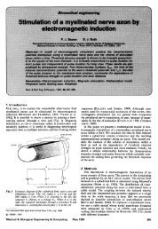
FIGURE 1.4 A schematic of the spin-echo method introduced<br />
by Hahn.<br />
γB (1.3)<br />
where B is the magnetic field that the spin is exposed<br />
<strong>to</strong> and γ is the gyromagnetic ratio – a constant specific<br />
<strong>to</strong> the nucleus under examination. <strong>In</strong> water, the hydrogen<br />
nucleus (i.e. the pro<strong>to</strong>n) has a gyromagnetic ratio<br />
value of approximately 2.68 10 8 rad/s/tesla. Spins<br />
that are initially coherent dephase due <strong>to</strong> fac<strong>to</strong>rs such<br />
as magnetic field inhomogeneities and dipolar interactions<br />
( Abragam, 1961 ) leading <strong>to</strong> a decay of the voltage<br />
(signal) induced in the receiver.<br />
As proposed by Edwin Hahn ( Hahn, 1950 ), and<br />
illustrated in Figure 1.4 , the dephasing due <strong>to</strong> magnetic<br />
field inhomogeneities can be reversed through a<br />
subsequent application of a 180 degree rf pulse, and<br />
the signal is reproduced. <strong>In</strong> this “ spin-echo ” experiment,<br />
the time between the first rf pulse and formation<br />
of the echo is called TE and it is twice the time<br />
between the two rf pulses, which is denoted by τ . The<br />
generated echo is detected by a receiver antenna (MR<br />
coil) and is used <strong>to</strong> produce spectra. Carefully devised<br />
sequences of rf pulses along with external magnetic<br />
field gradients linearly changing in space, enable the<br />
acquisition of magnetic resonance images. MR signal<br />
and image acquisition will be discussed in detail in<br />
Chapter 2.<br />
τ<br />
I. INTRODUCTION TO DIFFUSION <strong>MRI</strong>
6<br />
1. INTRODUCTION TO DIFFUSION MR<br />
The sensitivity of the spin-echo MR signal on<br />
molecular diffusion was recognized by Hahn. He<br />
reported a reduction of signal of the spin echo and<br />
explained it in terms of the dephasing of spins caused<br />
by translational diffusion within an inhomogeneous<br />
magnetic field ( Hahn, 1950 ). While he proposed that<br />
one could measure the diffusion coefficient of a solution<br />
containing spin-labeled molecules, he did not<br />
propose a direct method for doing so.<br />
A few years later, Carr and Purcell (1954) proposed<br />
a complete mathematical and physical framework for<br />
such a measurement using Hahn’s NMR spin-echo<br />
sequence. They realized that the echo magnitude<br />
could be sensitized solely <strong>to</strong> the effects of random<br />
molecular spreading caused by diffusion in a way<br />
that permits a direct measurement. The idea they<br />
employed is not very different from what is utilized in<br />
most current studies of diffusion-weighted imaging.<br />
Because a spin’s precession frequency is determined<br />
by the local magnetic field as implied by equation<br />
(1.3), if a “ magnetic field gradient ” is applied, spins<br />
that are at different locations experience different<br />
magnetic fields – hence they precess at different angular<br />
frequencies. After a certain time, the spins acquire<br />
different phase shifts depending on their location.<br />
Stronger gradients will lead <strong>to</strong> sharper phase changes<br />
across the specimen, yielding a higher sensitivity<br />
on diffusion. <strong>In</strong> most current clinical applications, a<br />
quantity called the “ b -value ” , which is proportional <strong>to</strong><br />
the square of the gradient strength, is used <strong>to</strong> characterize<br />
the level of the induced sensitivity on diffusion.<br />
<strong>In</strong> the scheme considered by Carr and Purcell, a<br />
constant magnetic field gradient is applied throughout<br />
the entire Hahn spin-echo experiment as shown<br />
in Figure 1.5 . Such an acquisition can be performed<br />
either in a spatially linear main field, or using another<br />
coil that is capable of creating a linear magnetic field<br />
on <strong>to</strong>p of the homogeneous field of the scanner ( B 0 ).<br />
<strong>In</strong> their description, at a particular time t , a particle<br />
situated at position x experiences a magnetic field of<br />
B 0 G x ( t ). If the particle is assumed <strong>to</strong> spend a short<br />
time, τ , at this point before moving <strong>to</strong> another location,<br />
it suffers a phase shift given by<br />
φ( xt ( )) ω( xt ( )) τ<br />
γ( B0 G x( t))<br />
τ<br />
(1.4)<br />
as a result of the Larmor precession at the field modified<br />
by the constant gradient. Here, the minus sign<br />
is necessary for pro<strong>to</strong>ns whose precession is in the<br />
clockwise direction on the plane perpendicular <strong>to</strong> the<br />
main magnetic field. Therefore, the net phase shift<br />
that influences the MR signal at t 2 τ is related <strong>to</strong><br />
the motional his<strong>to</strong>ry of the particles in the ensemble.<br />
By exploiting this phenomenon Carr and Purcell proposed<br />
MR sequences <strong>to</strong> sensitize the MR spin echo<br />
<strong>to</strong> the effects of diffusion, and developed a rigorous<br />
mathematical framework <strong>to</strong> measure the diffusion<br />
coefficient from such sequences. This elevated NMR<br />
as a “ gold standard ” for measuring molecular diffusion.<br />
An alternative mathematical formulation of the<br />
problem was introduced by Torrey (1956) who generalized<br />
the phenomenological Bloch equations ( Bloch,<br />
1946 ) <strong>to</strong> include the effects of diffusion.<br />
After about a decade, Stejskal and Tanner (1965)<br />
introduced many innovations that made modern diffusion<br />
measurements by NMR and <strong>MRI</strong> possible.<br />
First, they introduced the pulsed gradient spin-echo<br />
(PGSE) sequence, which replaced Carr and Purcell’s<br />
constant magnetic field with short duration gradient<br />
pulses as illustrated in Figure 1.6 . This allowed<br />
a clear distinction between the encoding time (pulse<br />
duration, δ ) and the diffusion time (separation of the<br />
two pulses, Δ ). A particularly interesting case of this<br />
pulse sequence that makes the problem considerably<br />
180°<br />
90°<br />
180°<br />
Rf<br />
90°<br />
Rf<br />
Gradient<br />
Signal<br />
FIGURE 1.5 A schematic of the spin-echo experiment in the<br />
presence of a constant field gradient discussed by Carr and Purcell.<br />
<strong>Diffusion</strong> taking place in the resulting inhomogeneous field gives<br />
rise <strong>to</strong> a decreased MR signal intensity.<br />
Gradient<br />
Signal<br />
G<br />
δ<br />
Δ<br />
FIGURE 1.6 A schematic of the pulsed field gradient spin-echo MR<br />
technique introduced by Stejskal and Tanner. The time between the<br />
application of the two gradient pulses, Δ , may be anywhere between<br />
10 ms and a few hundreds of milliseconds. The gradient pulse duration,<br />
δ , can vary between a few milliseconds <strong>to</strong> Δ , where when δ Δ ,<br />
the pulse sequence becomes the same as that in Figure 1.5 .<br />
δ<br />
I. INTRODUCTION TO DIFFUSION <strong>MRI</strong>
MAGNETIC RESONANCE AND DIFFUSION<br />
7<br />
simpler – from a theoretical point of view is obtained<br />
when the diffusion gradients are so short that diffusion<br />
taking place during the application of these<br />
pulses can be neglected. <strong>In</strong> this “ narrow pulse ”<br />
regime, the net phase change induced by the first gradient<br />
pulse is given simply by<br />
φ 1 qx 1<br />
(1.5)<br />
where x 1 is the position of the particle during the<br />
application of the first pulse and we ignore the phase<br />
change due <strong>to</strong> the B 0 field, which is constant for all<br />
spins in the ensemble. <strong>In</strong> the above expression all<br />
experimental parameters were combined in the quantity<br />
q γδ G , where δ and G are the duration and<br />
the magnitude of the gradient pulses, respectively.<br />
Similarly, if the particle is situated at position x 2 during<br />
the application of the second pulse, the net phase<br />
change due <strong>to</strong> the second pulse is given by<br />
φ 2 qx 2<br />
(1.6)<br />
The 180 degree rf pulse applied in between the two<br />
gradient pulses reverses the phase change that occurs<br />
prior <strong>to</strong> it, i.e. that induced by the first gradient pulse.<br />
Therefore, the aggregate phase change that the particle<br />
suffers is given by<br />
φ<br />
− φ qx<br />
( x) (1.7)<br />
2 1 2 1<br />
Clearly, if particles remained stationary, i.e. x 1 x 2 ,<br />
the net phase shift would vanish. <strong>In</strong> this case, and in<br />
the case in which all spins are displaced by the same<br />
constant amount, the magnitude of the echo will be<br />
unchanged (except for the T1 and T2 decay that is<br />
occurring throughout the sequence). However, if particles<br />
diffuse randomly throughout the excited volume,<br />
the phase increment they gain during the first<br />
period does not generally cancel the phase decrement<br />
they accrue during the second period. This incomplete<br />
cancellation results in phase dispersion or a spreading<br />
of phases among the randomly moving population of<br />
spins. Therefore, the overall signal, given by the sum<br />
of the magnetic moments of all spins, is attenuated<br />
due <strong>to</strong> the incoherence in the orientations of individual<br />
magnetic moments.<br />
It is more convenient <strong>to</strong> introduce a new quantity,<br />
E ( q ), called MR signal attenuation, than <strong>to</strong> deal with<br />
the MR signal itself. E ( q ) is obtained by dividing<br />
the diffusion-attenuated signal, S ( q ), by the signal in<br />
the absence of any gradients, S 0 S (0), i.e. E ( q ) S ( q ) /<br />
S 0 . Since relaxation-related signal attenuation is<br />
approximately independent of the applied diffusion<br />
gradients, dividing S ( q ) by S 0 eliminates the effects<br />
of relaxation, and the q -dependence of E ( q ) can be<br />
attributed solely <strong>to</strong> diffusion. The MR signal attenuation<br />
is then given by<br />
∫ ∫ , , d d<br />
iq( x x<br />
)<br />
ρ 1 1 2 2 1<br />
2 1<br />
Eq () ( x) Px ( x Δ ) e x x (1.8)<br />
where we employed two new quantities. The first of<br />
these, ρ ( x 1 ), is the spin density at the time of application<br />
of the first pulse quantifying the likelihood of<br />
finding a spin at location x 1 . <strong>In</strong> most applications, this<br />
function can be taken <strong>to</strong> be a constant throughout the<br />
water-filled region, where the value of the constant<br />
is determined by setting the integral of ρ ( x 1 ) equal <strong>to</strong><br />
unity. The second function that we used, P ( x 1 , x 2 , Δ ),<br />
is the diffusion propaga<strong>to</strong>r (Green’s function) that<br />
denotes the likelihood that a particle initially located<br />
at position x 1 will have ended up at x 2 after a time Δ –<br />
the separation of the two gradients. These two functions<br />
are related through the expression<br />
lim Px ( , x , t) ρ ( x)<br />
(1.9)<br />
t→∞<br />
1 2 1<br />
as when the diffusion time is very long, a spin can<br />
traverse <strong>to</strong> any location in space with the same probability.<br />
The remaining quantity in equation (1.8),<br />
iq( x x<br />
)<br />
2 1<br />
e cos( q( x2 x1)) isin( q( x2 x1 )) (1.10)<br />
where i 2 1, is the “ Fourier kernel ” that is used, e.g.,<br />
in obtaining the frequency response of a time-dependent<br />
signal. Here, the real (cosine) and imaginary (sine)<br />
components of the Fourier kernel represent, respectively,<br />
the x and y components of the two-dimensional<br />
magnetization vec<strong>to</strong>r on the plane perpendicular <strong>to</strong><br />
the main magnetic field, and the integration represents<br />
the summation over all possible displacements<br />
in the ensemble.<br />
If diffusion is free, the propaga<strong>to</strong>r is Gaussian<br />
and the MR signal attenuation is given by another<br />
Gaussian, Eq () e qD<br />
2 Δ . This expression is a special<br />
case of the more general Stejskal – Tanner relation,<br />
which takes the duration of the pulses in<strong>to</strong> consideration<br />
as well, given by<br />
Eq ()<br />
<br />
<br />
2<br />
qD( Δδ/3)<br />
e<br />
e<br />
bD<br />
(1.11)<br />
where b q 2 ( Δ δ / 3) ( γδ G ) 2 ( Δ δ / 3) is the b -value<br />
discussed above.<br />
Stejskal employed the above formalism for the case<br />
of free, anisotropic diffusion in the principal frame of<br />
reference ( Stejskal, 1965 ), where he used a “ tensor ” , i.e.<br />
a 3 3 matrix that represents the natural orientation of<br />
anisotropic diffusion with respect <strong>to</strong> the three axes of the<br />
labora<strong>to</strong>ry reference frame, which is determined by the<br />
I. INTRODUCTION TO DIFFUSION <strong>MRI</strong>
8<br />
1. INTRODUCTION TO DIFFUSION MR<br />
orthogonal orientations of the magnetic field gradients<br />
produced by the three gradient coils. A general scheme,<br />
called diffusion tensor imaging (DTI), was developed<br />
<strong>to</strong> measure the entire diffusion tensor (both its diagonal<br />
and off-diagonal elements) in each voxel within the labora<strong>to</strong>ry<br />
frame of reference ( Basser et al ., 1994 ).<br />
A. <strong>From</strong> the MR Signal Attenuation <strong>to</strong> the<br />
Average Propaga<strong>to</strong>r<br />
To glean the microstructural features of the specimen<br />
from the MR signal intensity, one may fit mathematical<br />
models <strong>to</strong> the acquired diffusion-weighted data.<br />
However, when the specimen’s microstructural features<br />
are not known a priori , or when the specimen exhibits<br />
considerable regional variability like in most applications<br />
of biological and medical imaging, an alternative<br />
approach that does not assume any particular model may<br />
be advantageous. For example, in the above discussion<br />
we have not employed any particular model and it would<br />
be desirable <strong>to</strong> obtain the local propaga<strong>to</strong>r, P (x 1 , x 2 , Δ ),<br />
employed in equation (1.8) from the MR signal. However,<br />
finite resolution of the images and the unavailability<br />
of the spin density function prohibit the inference of the<br />
local propaga<strong>to</strong>r directly from the MR signal.<br />
The difficulty associated with obtaining the local<br />
propaga<strong>to</strong>r can be overcome <strong>to</strong> some extent by introducing<br />
a net displacement variable x x 2 x 1 that<br />
makes it possible <strong>to</strong> write the simplified expression<br />
iqx<br />
Eq () ∫ Px (, Δ)<br />
e d x<br />
(1.12)<br />
where Px ( , Δ ) is the ensemble average propaga<strong>to</strong>r<br />
given by<br />
Px ( , Δ) ∫ ρ( x 1 ) Px ( 1 , x 1 x,<br />
Δ) d x 1 (1.13)<br />
This procedure, initially proposed by Stejskal<br />
(1965) , makes it possible <strong>to</strong> obtain an average propaga<strong>to</strong>r<br />
from the E ( q ) data by inverting the Fourier<br />
transform in equation (1.12). The propaga<strong>to</strong>r reconstructed<br />
in this fashion can be envisioned <strong>to</strong> be a<br />
“q -space image ” of the displacements ( Callaghan et al. ,<br />
1990 ). If the diffusion-sensitizing pulses are embedded<br />
in<strong>to</strong> imaging pro<strong>to</strong>cols and the average propaga<strong>to</strong>r<br />
is reconstructed at each voxel of the image,<br />
spatially localized displacement maps can be obtained<br />
( Callaghan et al. , 1988 ); this approach laid the foundation<br />
for developments of q -space NMR and <strong>MRI</strong><br />
( Callaghan, 1991 ) or equivalently, diffusion spectrum<br />
imaging (DSI) ( Tuch et al. , 2001 ; Wedeen et al. , 2005 ).<br />
The q -space imaging and DSI will be discussed in<br />
more detail in Chapters 4 and 7.<br />
III. DIFFUSION IN NEURAL TISSUE<br />
The incessant random motion of water molecules<br />
within the tissue is influenced by a variety of fac<strong>to</strong>rs<br />
such as restrictions due <strong>to</strong> cell membranes, cy<strong>to</strong>skele<strong>to</strong>n,<br />
and macromolecules ( Tanner and Stejskal, 1968 ).<br />
Figure 1.7 depicts how the cells may hinder the otherwise<br />
free motion of molecules. By employing the<br />
understanding of how microstructural features contribute<br />
<strong>to</strong> the overall diffusional process, it may be<br />
possible <strong>to</strong> obtain valuable information about the biological<br />
microstructure simply by observing the motion<br />
of water molecules. This is particularly important in<br />
the understanding of neural tissue for its no<strong>to</strong>riously<br />
complicated structure.<br />
Enhancing diffusive attenuation with the application<br />
of gradients, as we discussed for the case of spin echoes<br />
above, introduces a contrast mechanism different<br />
FIGURE 1.7 Biological cells may hinder the Brownian motion of extracellular water molecules (left). <strong>In</strong>side each cell, diffusion may be<br />
envisioned <strong>to</strong> be restricted by the cellular membranes (right).<br />
I. INTRODUCTION TO DIFFUSION <strong>MRI</strong>
REFERENCES<br />
9<br />
than that in relaxation-weighted magnetic resonance<br />
images. Such maps of the signal intensity S are called<br />
diffusion-weighted images. <strong>Diffusion</strong>-weighted images<br />
have been utilized extensively in neuroimaging since it<br />
was shown that ischemic strokes can be detected much<br />
earlier with diffusion-weighted images when compared<br />
<strong>to</strong> traditional T1 and T2 weighted magnetic resonance<br />
images ( Moseley et al. , 1990b ). This discovery<br />
has made diffusion-weighted imaging an indispensable<br />
<strong>to</strong>ol in the diagnosis and management of ischemic<br />
stroke.<br />
The central nervous system (CNS) comprises neuronal<br />
cells connected <strong>to</strong> each other through axons<br />
that function as transmission lines between different<br />
regions. An understanding of how the brain and<br />
the spinal cord function is not possible without the<br />
knowledge of how different ana<strong>to</strong>mical regions are<br />
connected <strong>to</strong> each other. Since water molecules tend<br />
<strong>to</strong> diffuse more freely along the direction of the fiber,<br />
if one can quantify the orientational preference of<br />
diffusion, it may be possible <strong>to</strong> relate it <strong>to</strong> the axonal<br />
orientations.<br />
<strong>In</strong> tissues, such as brain gray matter, where the<br />
measured apparent diffusivity is largely independent<br />
of the orientation of the tissue (i.e. isotropic) at the<br />
voxel length scale, it is usually sufficient <strong>to</strong> describe the<br />
diffusion characteristics with a single (scalar) apparent<br />
diffusion coefficient (ADC). However, in anisotropic<br />
media, such as white matter ( Henkelman et al. , 1994 ;<br />
Moseley et al. , 1990a, 1991 ) or skeletal and cardiac muscle<br />
( Cleveland et al. , 1976 ; Garrido et al. , 1994 ; Tanner,<br />
1979 ), where the measured diffusivity is known <strong>to</strong><br />
depend upon the orientation of the tissue, a single<br />
ADC does not adequately characterize the orientation-dependent<br />
water mobility. The next most complex<br />
model that describes anisotropic diffusion replaces the<br />
scalar ADC with a symmetric effective or apparent diffusion<br />
tensor of water, D (e.g. see Crank, 1975 ).<br />
The causes or biophysical basis of diffusion anisotropy<br />
in brain parenchyma and other tissues have<br />
not been fully elucidated, although most investiga<strong>to</strong>rs<br />
ascribe it <strong>to</strong> ordered, heterogeneous structures,<br />
such as large oriented extracellular and intracellular<br />
macromolecules, supermacromolecular structures,<br />
organelles, and membranes. Clearly, in the central<br />
nervous system (CNS), diffusion anisotropy in white<br />
matter is not simply caused by myelin, since several<br />
studies have shown that even before myelin is deposited,<br />
diffusion anisotropy can be measured using<br />
<strong>MRI</strong> ( Neil et al. , 1998 ; Beaulieu and Allen, 1994a, b ;<br />
Wimberger et al. , 1995 ). Thus, despite the fact that<br />
increases in myelin are temporally correlated with<br />
increases in diffusion anisotropy, structures other than<br />
the myelin sheath must significantly contribute <strong>to</strong><br />
diffusion anisotropy ( LeBihan et al. , 1993 ). This is<br />
important because the degree of diffusion anisotropy<br />
is not a quantitative measure or “ stain ” of myelin<br />
content ( Pierpaoli and Basser, 1996 ). The ana<strong>to</strong>mical<br />
determinants of diffusion anisotropy will be discussed<br />
in great detail in Chapter 5.<br />
IV. CONCLUDING REMARKS<br />
As water (or another spin-labeled molecule) undergoes<br />
diffusion, it also encounters barriers, macromolecules,<br />
sampling many different local environments.<br />
Collectively, the signal we measure in an MR experiment<br />
contains contributions from water motion in<br />
these various microenvironments. The challenge in<br />
diffusion NMR and <strong>MRI</strong> is <strong>to</strong> try <strong>to</strong> infer features of<br />
the local tissue ana<strong>to</strong>my, composition, and microstructure<br />
from MR displacement measurements. One great<br />
advantage of MR is that it permits one <strong>to</strong> probe tissue<br />
structure at different length scales ( Ö zarslan and<br />
Basser, 2008 ) – i.e. levels of hierarchical architectural<br />
organization ( Ö zarslan et al. , 2006 ). Specifically, while<br />
the mean-squared displacement of water is on the<br />
order of microns for typical MR experiments, these<br />
molecular motions are ensemble-averaged within a<br />
voxel, and then subsequently assembled in<strong>to</strong> multislice<br />
or 3D images of tissues and organs. Thus, this<br />
imaging modality permits us <strong>to</strong> study and elucidate<br />
complex structural features spanning length scales<br />
ranging from the macromolecular <strong>to</strong> the macroscopic –<br />
without the use of exogenous contrast agents.<br />
ACKNOWLEDGMENTS<br />
This research was supported by the <strong>In</strong>tramural<br />
Research Program of the Eunice Kennedy Shriver<br />
National <strong>In</strong>stitute of Child Health and Human<br />
Development.<br />
REFERENCES<br />
Abragam A ( 1961 ) The Principles of Nuclear Magnetism . Oxford :<br />
Clarendon Press .<br />
Basser PJ , Mattiello J , LeBihan D ( 1994 ) Estimation of the effective<br />
self-diffusion tensor from the NMR spin echo . J Magn Reson B<br />
103 ( 3 ) : 247 – 254 .<br />
Beaulieu C , Allen PS ( 1994 a ) Determinants of anisotropic water diffusion<br />
in nerves . Magn Reson Med 31 ( 4 ) : 394 – 400 .<br />
Beaulieu C , Allen PS ( 1994 b ) Water diffusion in the giant axon of the<br />
squid: implications for diffusion-weighted <strong>MRI</strong> of the nervous<br />
system . Magn Reson Med 32 ( 5 ) : 579 – 583 .<br />
Berg HC (ed.) ( 1983 ) Random Walks in Biology . Prince<strong>to</strong>n, NJ :<br />
Prince<strong>to</strong>n University Press .<br />
I. INTRODUCTION TO DIFFUSION <strong>MRI</strong>
10<br />
1. INTRODUCTION TO DIFFUSION MR<br />
Bloch F ( 1946 ) Nuclear induction . Phys Rev 70 ( 7,8 ) : 460 – 474 .<br />
Brown R ( 1828 ) A brief account of microscopical observations made<br />
in the months of June, July, and August, 1827, on the particles<br />
contained in the pollen of plants; and on the general existence<br />
of active molecules in organic and inorganic bodies . Phil Mag<br />
4 : 161 – 173 .<br />
Callaghan PT ( 1991 ) Principles of Nuclear Magnetic Resonance<br />
Microscopy . Oxford : Clarendon Press .<br />
Callaghan PT , Eccles CD , Xia Y ( 1988 ) NMR microscopy of<br />
dynamic displacements: k -space and q -space imaging . J Phys E<br />
21 : 820 – 822 .<br />
Callaghan PT , MacGowan D , Packer KJ , Zelaya FO ( 1990 ) Highresolution<br />
q -space imaging in porous structures . J Magn Reson<br />
90 : 177 – 182 .<br />
Carr HY , Purcell EM ( 1954 ) Effects of diffusion on free precession<br />
in nuclear magnetic resonance experiments . Phys Rev<br />
94 ( 3 ) : 630 – 638 .<br />
Chandrasekhar S ( 1943 ) S<strong>to</strong>chastic problems in physics and astronomy<br />
. Rev Mod Phys 15 ( 1 ) : 1 – 89 .<br />
Cleveland GG , Chang DC , Hazlewood CF , Rorschach HE ( 1976 )<br />
Nuclear magnetic resonance measurement of skeletal muscle:<br />
anisotropy of the diffusion coefficient of the intracellular water .<br />
Biophys J 16 ( 9 ) : 1043 – 1053 .<br />
Crank J ( 1975 ) Mathematics of <strong>Diffusion</strong> . Oxford : Clarendon Press .<br />
Einstein A ( 1905 ) Ü ber die von der molekularkinetischen Theorie<br />
der w ä rme gefordete Bewegung von in ruhenden Fl ü ssigkeiten<br />
suspendierten Teilchen . Ann Physik 4 : 549 – 560 .<br />
Einstein A ( 1926 ) <strong>In</strong>vestigations on the Theory of the Brownian<br />
Movement . New York : Dover Publications, <strong>In</strong>c .<br />
Fick A ( 1855 a ) Concerns diffusion and concentration gradient . Ann<br />
Phys Lpz 170 : 59 .<br />
Fick A ( 1855 b ) Ü ber diffusion . Ann Phys 94 : 59 .<br />
F ü rth R , Cowper AD (eds) ( 1956 ) <strong>In</strong>vestigations on the Theory of the<br />
Brownian Movement . New York : Dover Publications .<br />
Garrido L , Wedeen VJ , Kwong KK , Spencer UM , Kan<strong>to</strong>r HL ( 1994 )<br />
Anisotropy of water diffusion in the myocardium of the rat . Circ<br />
Res 74 ( 5 ) : 789 – 793 .<br />
Hahn EL ( 1950 ) Spin echoes . Phys Rev 80 : 580 – 594 .<br />
Henkelman RM , Stanisz GJ , Kim JK , Bronskill MJ ( 1994 ) Anisotropy<br />
of NMR properties of tissues . Magn Reson Med 32 : 592 – 601 .<br />
LeBihan D , Turner R , Douek P ( 1993 ) Is water diffusion restricted<br />
in human brain white matter? An echo-planar NMR imaging<br />
study . Neuroreport 4 ( 7 ) : 887 – 890 .<br />
Moseley ME , Cohen Y , Kucharczyk J , Min<strong>to</strong>rovitch J , Asgari HS ,<br />
Wendland MF , Tsuruda J , Norman D ( 1990 a ) <strong>Diffusion</strong>-weighted<br />
MR imaging of anisotropic water diffusion in cat central nervous<br />
system . Radiology 176 ( 2 ) : 439 – 445 .<br />
Moseley ME , Cohen Y , Min<strong>to</strong>rovitch J , Chileuitt L , Shimizu H ,<br />
Kucharczyk J , Wendland MF , Weinstein PR ( 1990 b ) Early detection<br />
of regional cerebral ischemia in cats: comparison of diffusion<br />
and T 2 -weighted <strong>MRI</strong> and spectroscopy . Magn Reson Med<br />
14 : 330 – 346 .<br />
Moseley ME , Kucharczyk J , Asgari HS , Norman D ( 1991 ) Anisotropy<br />
in diffusion-weighted <strong>MRI</strong> . Magn Reson Med 19 ( 2 ) : 321 – 326 .<br />
Neil JJ , Shiran SI , McKinstry RC , Schefft GL , Snyder AZ , Almli CR ,<br />
Akbudak E , Aronovitz JA , Miller JP , Lee BC , Conturo TE ( 1998 )<br />
Normal brain in human newborns: apparent diffusion coefficient<br />
and diffusion anisotropy measured by using diffusion tensor<br />
MR imaging . Radiology 209 ( 1 ) : 57 – 66 .<br />
Ö zarslan E , Basser PJ ( 2008 ) Microscopic anisotropy revealed by<br />
NMR double pulsed field gradient experiments with arbitrary<br />
timing parameters . J Chem Phys 128 ( 15 ) : 154511 .<br />
Ö zarslan E , Basser PJ , Shepherd TM , Thelwall PE , Vemuri BC ,<br />
Blackband SJ ( 2006 ) Observation of anomalous diffusion in<br />
excised tissue by characterizing the diffusion-time dependence<br />
of the MR signal . J Magn Reson 183 ( 2 ) : 315 – 323 .<br />
Pierpaoli C , Basser PJ ( 1996 ) Toward a quantitative assessment of<br />
diffusion anisotropy . Magn Reson Med 36 ( 6 ) : 893 – 906 .<br />
Smoluchowski MR ( 1906 ) Zur kinetischen Theorie der Brownschen<br />
Molekularbewegung und der Suspensionen . Ann Phys<br />
21 : 756 – 780 .<br />
Stejskal EO ( 1965 ) Use of spin echoes in a pulsed magnetic-field gradient<br />
<strong>to</strong> study anisotropic, restricted diffusion and flow . J Chem<br />
Phys 43 ( 10 ) : 3597 – 3603 .<br />
Stejskal EO , Tanner JE ( 1965 ) Spin diffusion measurements: spin<br />
echoes in the presence of a time-dependent field gradient .<br />
J Chem Phys 42 ( 1 ) : 288 – 292 .<br />
Tanner JE ( 1979 ) Self diffusion of water in frog muscle . Biophys<br />
J 28 ( 1 ) : 107 – 116 .<br />
Tanner JE , Stejskal EO ( 1968 ) Restricted self-diffusion of pro<strong>to</strong>ns<br />
in colloidal systems by the pulsed-gradient, spin-echo method .<br />
J Chem Phys 49 ( 4 ) : 1768 – 1777 .<br />
Torrey HC ( 1956 ) Bloch equations with diffusion terms . Phys Rev<br />
104 ( 3 ) : 563 – 565 .<br />
Tuch DS, Wiegell MR, Reese TG, Belliveau JW, Wedeen VJ (2001)<br />
Measuring cortico-cortical connectivity matrices with diffusion<br />
spectrum imaging. <strong>In</strong>: Proc. of the 9th Annual Meeting of ISMRM ,<br />
Glasgow, p. 502.<br />
Wedeen VJ , Hagmann P , Tseng W-YI , Reese TG , Weisskoff RM ( 2005 )<br />
Mapping complex tissue architecture with diffusion spectrum<br />
magnetic resonance imaging . Magn Reson Med 54 ( 6 ) : 1377 – 1386 .<br />
Wimberger DM , Roberts TP , Barkovich AJ , Prayer LM , Moseley ME ,<br />
Kucharczyk J (1995 ) Identification of “premyelination ” by diffusionweighted<br />
<strong>MRI</strong> . J Comput Assist Tomogr 19 ( 1 ) : 28 – 33 .<br />
I. INTRODUCTION TO DIFFUSION <strong>MRI</strong>