Slides Chapter 1. Measure Theory and Probability
Slides Chapter 1. Measure Theory and Probability
Slides Chapter 1. Measure Theory and Probability

You also want an ePaper? Increase the reach of your titles
YUMPU automatically turns print PDFs into web optimized ePapers that Google loves.
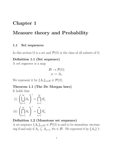
<strong>Chapter</strong> 1<br />
<strong>Measure</strong> theory <strong>and</strong> <strong>Probability</strong><br />
<strong>1.</strong>1 Set sequences<br />
In this section Ω is a set <strong>and</strong> P(Ω) is the class of all subsets of Ω.<br />
Definition <strong>1.</strong>1 (Set sequence)<br />
A set sequence is a map<br />
IN → P(Ω)<br />
n A n<br />
We represent it by {A n } n∈IN ∈ P(Ω).<br />
Theorem <strong>1.</strong>1 (The De Morgan laws)<br />
It holds that<br />
( ∞<br />
) c<br />
⋃ ∞⋂<br />
(i) A n = A c n.<br />
(ii)<br />
n=1<br />
(<br />
⋂ ∞<br />
) c<br />
A n =<br />
n=1<br />
n=1<br />
∞⋃<br />
A c n.<br />
n=1<br />
Definition <strong>1.</strong>2 (Monotone set sequence)<br />
A set sequence {A n } n∈IN ∈ P(Ω) is said to be monotone increasing<br />
if<strong>and</strong>onlyifA n ⊆ A n+1 ,∀n ∈ IN. Werepresentitby{A n } ↑.<br />
1
<strong>1.</strong><strong>1.</strong> SET SEQUENCES<br />
When A n ⊇ A n+1 , ∀n ∈ IN, the sequence is said to be monotone<br />
decreasing, <strong>and</strong> we represent it by {A n } ↓.<br />
Example <strong>1.</strong>1 Consider the sequences defined by:<br />
(i) A n = (−n,n), ∀n ∈ IN. This sequence is monotone increasing,<br />
since ∀n ∈ IN,<br />
A n = (−n,n) ⊂ (−(n+1),n+1) = A n+1 .<br />
(ii) B n = (−1/n,1+1/n), ∀n ∈ IN. This sequence is monotone<br />
decreasing, since ∀n ∈ IN,<br />
B n = (−1/n,1+1/n) ⊃ (−1/(n+1),1+1/(n+1)) = B n+1 .<br />
Definition <strong>1.</strong>3 (Limit of a set sequence)<br />
(i) We call lower limit of {A n }, <strong>and</strong> we denote it limA n , to the<br />
set of points of Ω that belong to all A n s except for a finite<br />
number of them.<br />
(ii) We call upper limit of {A n }, <strong>and</strong> we denote it limA n , to the<br />
set of points of Ω that belong to infinite number of A n s. It<br />
is also said that A n occurs infinitely often (i.o.), <strong>and</strong> it is<br />
denoted also limA n = A n i.o.<br />
Example <strong>1.</strong>2 If ω ∈ A 2n , ∀n ∈ IN, then ω ∈ limA n but ω /∈<br />
limA n since there is an infinite number of A n s to which ω does not<br />
belong, {A 2n−1 } n∈IN .<br />
Proposition <strong>1.</strong>1 (Another characterization of limit of<br />
a set sequence)<br />
∞⋃ ∞⋂<br />
(i) limA n =<br />
k=1n=k<br />
A n<br />
ISABEL MOLINA 2
<strong>1.</strong><strong>1.</strong> SET SEQUENCES<br />
(ii) limA n =<br />
∞⋂<br />
∞⋃<br />
k=1n=k<br />
A n<br />
Proposition <strong>1.</strong>2 (Relationbetweenlower <strong>and</strong>upperlimits)<br />
The lower <strong>and</strong> upper limits of a set sequence {A n } satisfy<br />
limA n ⊆ limA n<br />
Definition <strong>1.</strong>4 (Convergence)<br />
A set sequence {A n } converges if <strong>and</strong> only if<br />
Then, we call limit of {A n } to<br />
limA n = limA n .<br />
lim<br />
n→∞ A n = limA n = limA n .<br />
Definition <strong>1.</strong>5 (Inferior/Superior limit of a sequence of<br />
real numbers)<br />
Let {a n } n∈IN ∈ IR be a sequence. We define:<br />
(i) liminf a n = sup inf a n;<br />
n→∞ k n≥k<br />
(ii) limsup<br />
n→∞<br />
a n = inf sup a n .<br />
k n≥k<br />
Proposition <strong>1.</strong>3 (Convergence of monotoneset sequences)<br />
Any monotone (increasing of decreasing) set sequence converges,<br />
<strong>and</strong> it holds:<br />
(i) If {A n } ↑, then lim<br />
n→∞<br />
A n =<br />
(ii) If {A n } ↓, then lim<br />
n→∞<br />
A n =<br />
∞⋃<br />
A n .<br />
n=1<br />
∞⋂<br />
A n .<br />
n=1<br />
ISABEL MOLINA 3
<strong>1.</strong><strong>1.</strong> SET SEQUENCES<br />
Example <strong>1.</strong>3 Obtain the limits of the following set sequences:<br />
(i) {A n }, where A n = (−n,n), ∀n ∈ IN.<br />
(ii) {B n }, where B n = (−1/n,1+1/n), ∀n ∈ IN.<br />
(i) By the previous proposition, since {A n } ↑, then<br />
∞⋃ ∞⋃<br />
lim A n = A n = (−n,n) = IR.<br />
n→∞<br />
n=1<br />
n=1<br />
(ii) Again, using the previous proposition, since {A n } ↓, then<br />
∞⋂ ∞⋂<br />
(<br />
lim B n = B n = − 1<br />
n→∞ n ,1+ 1 )<br />
= [0,1].<br />
n<br />
Problems<br />
n=1<br />
<strong>1.</strong> Prove Proposition <strong>1.</strong><strong>1.</strong><br />
n=1<br />
2. Define sets of real numbers as follows. Let A n = (−1/n,1] if<br />
n is odd, <strong>and</strong> A n = (−1,1/n] if n is even. Find limA n <strong>and</strong><br />
limA n .<br />
3. Prove Proposition <strong>1.</strong>2.<br />
4. Prove Proposition <strong>1.</strong>3.<br />
5. Let Ω = IR 2 <strong>and</strong> A n the interior of the circle with center at<br />
the point ((−1) n /n,0) <strong>and</strong> radius <strong>1.</strong> Find limA n <strong>and</strong> limA n .<br />
6. Prove that (limA n ) c = limA c n <strong>and</strong> (limA n ) c = limA c n.<br />
7. Using the De Morgan laws <strong>and</strong> Proposition <strong>1.</strong>3, prove that if<br />
{A n } ↑ A, then {A c n} ↓ A c while if {A n } ↓ A, then {A c n} ↑<br />
A c .<br />
ISABEL MOLINA 4
<strong>1.</strong>2. STRUCTURES OF SUBSETS<br />
8. Let{x n }beasequenceofrealnumbers<strong>and</strong>letA n = (−∞,x n ).<br />
What is the connection between liminf x n <strong>and</strong> limA n ? Similarly<br />
between limsupx n <strong>and</strong> limA n .<br />
n→∞<br />
n→∞<br />
<strong>1.</strong>2 Structures of subsets<br />
AprobabilityfunctionwillbeafunctiondefinedovereventsorsubsetsofasamplespaceΩ.<br />
Itisconvenienttoprovidea“good”structure<br />
to these subsets, which in turn will provide “good” properties<br />
to the probability function. In this section we study collections of<br />
subsets of a set Ω with a good structure.<br />
Definition <strong>1.</strong>6 (Algebra)<br />
An algebra (also called field) A over a set Ω is a collection of<br />
subsets of Ω that has the following properties:<br />
(i) Ω ∈ A;<br />
(ii) If A ∈ A, then A c ∈ A;<br />
(iii) If A 1 ,A 2 ,...,A n ∈ A, then<br />
n⋃<br />
A i ∈ A.<br />
An algebra over Ω contains both Ω <strong>and</strong> ∅. It also contains all<br />
finite unions <strong>and</strong> intersections of sets from A. We say that A is<br />
closed under complementation, finite union <strong>and</strong> finite intersection.<br />
Extending property (iii) to an infinite sequence of elements of A<br />
we obtain a σ-algebra.<br />
Definition <strong>1.</strong>7 (σ-algebra)<br />
A σ-algebra (or σ-field) A over a set Ω is a collection of subsets of<br />
Ω that has the following properties:<br />
i=1<br />
ISABEL MOLINA 5
<strong>1.</strong>2. STRUCTURES OF SUBSETS<br />
(i) Ω ∈ A;<br />
(ii) If A ∈ A, then A c ∈ A;<br />
(iii) IfA 1 ,A 2 ...isasequenceofelementsofA,then∪ ∞ n=1A n ∈ A.<br />
Thus, a σ-algebra is closed under countable union. It is also<br />
closed under countable intersection. Moreover, if A is an algebra,<br />
a countable union of sets in A can be expressed as the limit of<br />
n⋃<br />
an increasing sequence of sets, the finite unions A i . Thus, a<br />
σ-algebra is an algebra that is closed under limits of increasing<br />
sequences.<br />
Example <strong>1.</strong>4 The smallest σ-algebra is {∅,Ω}. The smallest<br />
σ-algebra that contains a subset A ⊂ Ω is {∅,A,A c ,Ω}. It is<br />
contained in any other σ-algebra containing A. The collection of<br />
all subsets of Ω, P(Ω), is a well known algebra called the algebra<br />
of the parts of Ω.<br />
Definition <strong>1.</strong>8 (σ-algebra spanned by a collection C of<br />
events)<br />
Given a collection of sets C ⊂ P(Ω), we define the σ-algebra<br />
spanned by C, <strong>and</strong> we denote it by σ(C), as the smallest σ-algebra<br />
that contains C.<br />
Remark <strong>1.</strong>1 For each C, the σ-algebra spanned by C, σ(C), always<br />
exists, since A C is the intersection of all σ-algebras that contain<br />
C <strong>and</strong> at least P(Ω) ⊃ C is a σ-algebra.<br />
When Ω is finite or countable, it is common to work with the<br />
σ-algebra P(Ω), so we will use this one unless otherwise stated. In<br />
the case Ω = IR, later we will consider probability measures <strong>and</strong><br />
we will want to obtain probabilities of intervals. Thus, we need a<br />
i=1<br />
ISABEL MOLINA 6
<strong>1.</strong>2. STRUCTURES OF SUBSETS<br />
σ-algebra containing all intervals. The Borel σ-algebra is based on<br />
this idea, <strong>and</strong> it will be used by default when Ω = IR.<br />
Definition <strong>1.</strong>9 (Borel σ-algebra)<br />
Consider the sample space Ω = IR <strong>and</strong> the collection of intervals<br />
of the form<br />
I = {(−∞,a] : a ∈ IR}.<br />
We define the Borel σ-algebra over IR, represented by B, as the<br />
σ-algebra spanned by I.<br />
The Borel σ-algebra B contains all complements, countable intersections<br />
<strong>and</strong> unions of elements of I. In particular, B contains<br />
all types of intervals <strong>and</strong> isolated points of IR, although B is not<br />
equal to P(IR). For example,<br />
• (a,∞) ∈ B, since (a,∞) = (−∞,a] c , <strong>and</strong> (−∞,a] ∈ IR.<br />
• (a,b] ∈ IR, ∀a < b, since this interval can be expressed as<br />
(a,b] = (−∞,b]∩(a,∞), where (−∞,b] ∈ B <strong>and</strong> (a,∞) ∈<br />
B.<br />
∞⋂<br />
• {a} ∈ B,∀a ∈ IR,since{a} =<br />
(a− 1 ]<br />
n ,a ,whichbelongs<br />
to B.<br />
When the sample space Ω is continuous but is a subset of IR,<br />
we need a σ-algebra restricted to subsets of Ω.<br />
Definition <strong>1.</strong>10 (Restricted Borel σ-algebra )<br />
Let A ⊂ IR. We define the Borel σ-algebra restricted to A as the<br />
collection<br />
B A = {B ∩A : B ∈ B}.<br />
n=1<br />
ISABEL MOLINA 7
<strong>1.</strong>3. SET FUNCTIONS<br />
In the following we define the space over which measures, including<br />
probability measures, will be defined. This space will be<br />
the one whose elements will be suitable to “measure”.<br />
Definition <strong>1.</strong>11 (<strong>Measure</strong> space)<br />
The pair (Ω,A), where Ω is a sample space <strong>and</strong> A is an algebra<br />
over Ω, is called measurable space.<br />
Problems<br />
<strong>1.</strong> Let A,B ∈ Ω with A ∩ B = ∅. Construct the smallest σ-<br />
algebra that contains A <strong>and</strong> B.<br />
2. Prove that an algebra over Ω contains all finite intersections<br />
of sets from A.<br />
3. Prove that a σ-algebra over Ω contains all countable intersections<br />
of sets from A.<br />
4. Prove that a σ-algebra is an algebra that is closed under limits<br />
of increasing sequences.<br />
5. Let Ω = IR. Let A be the class of all finite unions of disjoint<br />
elements from the set<br />
C = {(a,b],(−∞,a],(b,∞);a ≤ b}<br />
Prove that A is an algebra.<br />
<strong>1.</strong>3 Set functions<br />
In the following A is an algebra <strong>and</strong> we consider the extended real<br />
line given by IR = IR∪{−∞,+∞}.<br />
ISABEL MOLINA 8
<strong>1.</strong>3. SET FUNCTIONS<br />
Definition <strong>1.</strong>12 (Additive set function)<br />
A set function φ : A → IR is additive if it satisfies:<br />
( n<br />
)<br />
⋃<br />
For all{A i } n i=1 ∈ AwithA i ∩A j = ∅, i ≠ j, φ A i =<br />
i=1<br />
n∑<br />
φ(A i ).<br />
We will assume that +∞ <strong>and</strong> −∞ cannot both belong to the<br />
range of φ. We will exclude the cases φ(A) = +∞ for all A ∈ A<br />
<strong>and</strong> φ(A) = −∞ for all A ∈ A. Extending the definition to an<br />
infinite sequence, we obtain a σ-additive set function.<br />
Definition <strong>1.</strong>13 (σ-additive set function)<br />
A set function φ : A → IR is σ-additive if it satisfies:<br />
For all {A n } n∈IN ∈ A with A i ∩A j = ∅, i ≠ j,<br />
( ∞<br />
)<br />
⋃ ∞∑<br />
φ A n = φ(A n ).<br />
n=1<br />
Observe that a σ-additive set function is well defined, since the<br />
infinite union of sets of A belongs to A because A is a σ-algebra.<br />
It is easy to see that an additive function satisfies µ(∅) = 0. Moreover,<br />
countable additivity implies finite additivity.<br />
n=1<br />
Definition <strong>1.</strong>14 (<strong>Measure</strong>)<br />
A set function φ : A → IR is a measure if<br />
(a) φ is σ-additive;<br />
(b) φ(A) ≥ 0, ∀A ∈ A.<br />
Definition <strong>1.</strong>15 (<strong>Probability</strong> measure)<br />
A measure µ with µ(Ω) = 1 is called a probability measure.<br />
i=1<br />
ISABEL MOLINA 9
<strong>1.</strong>3. SET FUNCTIONS<br />
Example <strong>1.</strong>5 (Counting measure)<br />
Let Ω be any set <strong>and</strong> consider the σ-algebra of the parts of Ω,<br />
P(Ω). Define µ(A) as the number of points of A. The set function<br />
µ is a measure known as the counting measure.<br />
Example <strong>1.</strong>6 (<strong>Probability</strong> measure)<br />
Let Ω = {x 1 ,x 2 ,...} be a finite or countably infinite set, <strong>and</strong> let<br />
p 1 ,p 2 ,..., be nonnegative numbers. Consider the σ-algebra of the<br />
parts of Ω, P(Ω), <strong>and</strong> define<br />
µ(A) = ∑ x i ∈Ap i .<br />
Thesetfunctionµisaprobabilitymeasureif<strong>and</strong>onlyif ∑ ∞<br />
i=1 p i =<br />
<strong>1.</strong><br />
Example <strong>1.</strong>7 (Lebesgue measure)<br />
A well known measure defined over (IR,B), which assigns to each<br />
element of B its length, is the Lebesgue measure, denoted here as<br />
λ. For an interval, either open, close or semiclosed, the Lebesgue<br />
measure is the length of the interval. For a single point, the<br />
Lebesgue measure is zero.<br />
Definition <strong>1.</strong>16 (σ-finite set function)<br />
A set function φ : A → IR is σ-finite if ∀A ∈ A, there exists a<br />
sequence {A n } n∈IN of disjoint elements of A with φ(A n ) < ∞ ∀n,<br />
whose union covers A, that is,<br />
∞⋃<br />
A ⊆ A n .<br />
n=1<br />
Definition <strong>1.</strong>17 (<strong>Measure</strong> space)<br />
The triplet (Ω,A,µ), where Ω is a sample space, A is an algebra<br />
<strong>and</strong> µ is a measure defined over (Ω,A), is called measure space.<br />
ISABEL MOLINA 10
<strong>1.</strong>3. SET FUNCTIONS<br />
Definition <strong>1.</strong>18 (Absolutely continuous measure with<br />
respect to another)<br />
A measure µ on Borel subsets of the real line is absolutely continuous<br />
with respect to another measure λ if λ(A) = 0 implies that<br />
µ(A) = 0. It is also said that µ is dominated by λ, <strong>and</strong> written as<br />
µ
<strong>1.</strong>4. PROBABILITY MEASURES<br />
defined on an algebra A, then for all A 1 ,...,A n ∈ A,<br />
( n<br />
)<br />
⋃ n∑<br />
µ A i ≤ µ(A i ).<br />
i=1<br />
5. Prove that for any measure µ defined on an algebra A, then<br />
for all A 1 ,...,A n ∈ A such that ⋃ ∞<br />
n=1 A n ∈ A,<br />
( ∞<br />
)<br />
⋃ ∞∑<br />
µ A n ≤ µ(A n ).<br />
n=1<br />
<strong>1.</strong>4 <strong>Probability</strong> measures<br />
i=1<br />
n=1<br />
Definition <strong>1.</strong>19 (R<strong>and</strong>om experiment)<br />
A r<strong>and</strong>om experiment is a process for which:<br />
• the set of possible results is known;<br />
• its result cannot be predicted without error;<br />
• if we repeat it in identical conditions, the result can be different.<br />
Definition <strong>1.</strong>20 (Elementary event, sample space, event)<br />
The possible results of the r<strong>and</strong>om experiment that are indivisible<br />
are called elementary events. The set of elementary events is<br />
known as sample space, <strong>and</strong> it will be denoted Ω. An event A is a<br />
subset of Ω, such that once the r<strong>and</strong>om experiment is carried out,<br />
we can say that A “has occurred” if the result of the experiment<br />
is contained in A.<br />
Example <strong>1.</strong>8 Examples of r<strong>and</strong>om experiments are:<br />
(a) Tossing a coin. The sample space is Ω = {“head”,“tail”}.<br />
Events are: ∅, {“head”}, {“tail”}, Ω.<br />
ISABEL MOLINA 12
<strong>1.</strong>4. PROBABILITY MEASURES<br />
(b) ObservingthenumberoftrafficaccidentsinaminuteinSpain.<br />
The sample space is Ω = IN ∪{0}.<br />
(c) Drawing a Spanish woman aged between 20 <strong>and</strong> 40 <strong>and</strong> measuring<br />
her weight (in kgs.). The sample space is Ω = [m,∞),<br />
were m is the minimum possible weight.<br />
We will require that the collection of events has a structure of<br />
σ-algebra. This will make possible to obtain the probability of all<br />
complements, unions <strong>and</strong> intersections of events. The probabilities<br />
will be set functions defined over a measurable space composed by<br />
the sample space Ω <strong>and</strong> a σ-algebra of subsets of Ω.<br />
Example <strong>1.</strong>9 For the experiment (a) described in Example <strong>1.</strong>8,<br />
a measurable space is:<br />
Ω = {“head”,“tail”}, A = {∅,{“head”},{“tail”},Ω}.<br />
For the experiment (b), the sample space is Ω = IN ∪{0}. If we<br />
take the σ-algebra P(Ω), then (Ω,P(Ω)) is a measurable space.<br />
Finally, for the experiment (c), with sample space Ω = [m,∞) ⊂<br />
IR, a suitable σ-algebra is the Borel σ-algebra restricted to Ω,<br />
B [m,∞) .<br />
Definition <strong>1.</strong>21 (Axiomatic definition of probability by<br />
Kolmogoroff)<br />
Let (Ω,A) be a measurable space, where Ω is a sample space <strong>and</strong><br />
A is a σ-algebra over Ω. A probability function is a set function<br />
P : A → [0,1] that satisfies the following axioms:<br />
(i) P(Ω) = 1;<br />
(ii) For any sequence A 1 ,A 2 ,... of disjoint elements of A, it holds<br />
( ∞<br />
)<br />
⋃ ∞∑<br />
P A n = P(A n ).<br />
n=1<br />
n=1<br />
ISABEL MOLINA 13
<strong>1.</strong>4. PROBABILITY MEASURES<br />
By axiom (ii), a probability function is a measure for which the<br />
measure of the sample space Ω is <strong>1.</strong> The triplet (Ω,A,P), where<br />
P is a probability P, is called probability space.<br />
Example <strong>1.</strong>10 Fortheexperiment(a)describedinExample<strong>1.</strong>8,<br />
with the measurable space (Ω,A), where<br />
define<br />
Ω = {“head”,“tail”}, A = {∅,{“head”},{“tail”},Ω},<br />
P 1 (∅) = 0, P 1 ({“head”}) = p, P 1 ({“tail”}) = 1−p, P 1 (Ω) = 1,<br />
where p ∈ [0,1]. This function verifies the axioms of Kolmogoroff.<br />
Example <strong>1.</strong>11 For the experiment (b) described is Example <strong>1.</strong>8,<br />
with the measurable space (Ω,P(Ω)), define:<br />
• For the elementary events, the probability is<br />
P({0}) = 0.131, P({1}) = 0.272, P({2}) = 0.27, P({3}) = 0.183,<br />
P({4}) = 0.09, P({5}) = 0.012, P({6}) = 0.00095, P({7}) = 0.00005,<br />
P(∅) = 0, P({i}) = 0, ∀i ≥ 8.<br />
• For other events, the probability is defined as the sum of the<br />
probabilities of the elementary events contains in that event,<br />
that is, if A = {a 1 ,...,a n }, where a i ∈ Ω are the elementary<br />
events, the probability of A is<br />
n∑<br />
P(A) = P({a i }).<br />
i=1<br />
This function verifies the axioms of Kolmogoroff.<br />
Proposition <strong>1.</strong>4 (Properties of the probability)<br />
The following properties are consequence of the axioms of Kolmogoroff:<br />
ISABEL MOLINA 14
<strong>1.</strong>4. PROBABILITY MEASURES<br />
(i) P(∅) = 0;<br />
(ii) Let A 1 ,A 2 ,...,A n ∈ A with A i ∩A j = ∅, i ≠ j. Then,<br />
P<br />
(<br />
⋃ n<br />
)<br />
A i =<br />
i=1<br />
n∑<br />
P(A i ).<br />
i=1<br />
(iii) ∀A ∈ A, P(A) ≤ <strong>1.</strong><br />
(iv) ∀A ∈ A, P(A c ) = 1−P(A).<br />
(v) For A,B ∈ A with A ⊆ B, it holds P(A) ≤ P(B).<br />
(vi) Let A,B ∈ A be two events. Then<br />
P(A∪B) = P(A)+P(B)−P(A∩B).<br />
(vii) Let A 1 ,A 2 ,...,A n ∈ A be events. Then<br />
( n<br />
)<br />
⋃ n∑ n∑<br />
P A i = P(A i )− P(A i1 ∩A i2 )<br />
i=1 i=1 i 1 ,i 2 =1<br />
i 1
<strong>1.</strong>4. PROBABILITY MEASURES<br />
Proposition <strong>1.</strong>6 (Sequential continuity of the probability)<br />
Let(Ω,A,P)beaprobabilityspace. Then,foranysequence{A n }<br />
of events from A it holds<br />
P<br />
(<br />
lim<br />
n→∞ A n<br />
)<br />
= lim<br />
n→∞<br />
P(A n ).<br />
Example <strong>1.</strong>12 Considerther<strong>and</strong>omexperimentofselectingr<strong>and</strong>omly<br />
a number from [0,1]. Then the sample space is Ω = [0,1].<br />
Consider also the Borel σ-algebra restricted to [0,1] <strong>and</strong> define the<br />
function<br />
g(x) = P([0,x]), x ∈ (0,1).<br />
Proof that g is always right continuous, for each probability measure<br />
P that we choose.<br />
Example <strong>1.</strong>13 (Construction of a probability measure<br />
for countable Ω)<br />
If Ω is finite or countable, the σ-algebra that is typically chosen<br />
is P(Ω). In this case, in order to define a probability function, it<br />
suffices to define the probabilities of the elementary events {a i } as<br />
P({a i }) = p i , ∀a i ∈ Ω with the condition that ∑ i p i = 1, p i ≥ 0,<br />
∀i. Then, ∀A ⊂ Ω,<br />
P(A) = ∑ a i ∈A<br />
P({a i }) = ∑ a i ∈Ap i .<br />
Example <strong>1.</strong>14 (Construction of a probability measure<br />
in (IR,B))<br />
How can we construct a probability measure in (IR,B)? In general,<br />
it is not possible to define a probability measure by assigning<br />
directly a numerical value to each A ∈ B, since then probably the<br />
axioms of Kolmogoroff will not be satisfied.<br />
ISABEL MOLINA 16
<strong>1.</strong>4. PROBABILITY MEASURES<br />
For this, we will first consider the collection of intervals<br />
C = {(a,b],(−∞,b],(a,+∞) : a < b}. (<strong>1.</strong>1)<br />
We start by assigning values of P to intervals from C, by ensuring<br />
that P is σ-additive on C. Then, we consider the algebra F obtained<br />
by doing finite unions of disjoint intervals from C <strong>and</strong> we<br />
extend P to F. The extended function will be a probability measureon(IR,F).<br />
Finally,thereisauniqueextensionofaprobability<br />
measure from F to σ(F) = B, see the following propositions.<br />
Proposition <strong>1.</strong>7 Consider the collection of all finite unions of<br />
disjoint intervals from C in (<strong>1.</strong>1),<br />
{ n<br />
}<br />
⋃<br />
F = A i : A i ∈ C, A i disjoint .<br />
Then F is an algebra.<br />
i=1<br />
Next we extend P from C to F as follows.<br />
Proposition <strong>1.</strong>8 (Extensionof theprobabilityfunction)<br />
(a) For all A ∈ F, since A = ⋃ n<br />
i=1 (a i,b i ], with a i ,b i ∈ IR ∪<br />
{−∞,+∞}, let us define<br />
n∑<br />
P 1 (A) = P(a i ,b i ].<br />
i=1<br />
Then, P 1 is a probability measure over (IR,F).<br />
(b) For all A ∈ C, it holds that P(A) = P 1 (A).<br />
Observe that B = σ(F). Finally, can we extend P from F to<br />
B = σ(F)? If the answer is positive, is the extension unique? The<br />
next theorem gives the answer to these two questions.<br />
ISABEL MOLINA 17
<strong>1.</strong>4. PROBABILITY MEASURES<br />
Theorem <strong>1.</strong>2 (Caratheodory’s Extension Theorem)<br />
Let(Ω,A,P)beaprobabilityspace, whereAisanalgebra. Then,<br />
P can be extended from A to σ(A), <strong>and</strong> the extension is unique<br />
(i.e., there exists a unique probability measure ˆP over σ(A) with<br />
ˆP(A) = P(A), ∀A ∈ A).<br />
TheextensionofP fromF toσ(F) = B isdonebysteps. First,<br />
P is extended to the collection of the limits of increasing sequences<br />
ofeventsinF,denotedC. ItholdsthatC ⊃ F <strong>and</strong>C ⊃ σ(F) = B<br />
(Monotone Class Theorem). The probability of each event A from<br />
C is defined as the limit of the probabilities of the sequences of<br />
events from F that converge to A. Afterwards, P is extended<br />
to the σ-algebra of the parts of IR. For each subset A ∈ P(IR),<br />
the probability is defined as the infimum of the probabilities of<br />
the events in C that contain A. This extension is not countably<br />
additive on P(IR), only on a smaller σ-algebra, so P it is not a<br />
probability measure on (IR,P(IR)). Finally, a σ-algebra in which<br />
P is a probability measure is defined as the collection H of subsets<br />
H ⊂ Ω, for which P(H)+P(H c ) = <strong>1.</strong> This collection is indeed a<br />
σ-algebra that contains C <strong>and</strong> P is a probability measure on it. It<br />
holds that σ(F) = B ⊂ H <strong>and</strong> P restricted to σ(F) = B is also a<br />
probability measure on (IR,B).<br />
Problems<br />
<strong>1.</strong> ProvethepropertiesoftheprobabilitymeasuresinProposition<br />
<strong>1.</strong>4.<br />
2. Prove Bool’s inequality in Proposition <strong>1.</strong>4.<br />
3. Prove the Sequential Continuity of the probability in Proposition<br />
<strong>1.</strong>6.<br />
ISABEL MOLINA 18
<strong>1.</strong>5. OTHER DEFINITIONS OF PROBABILITY<br />
<strong>1.</strong>5 Other definitions of probability<br />
WhenΩisfinite,sayΩ = {a 1 ,...,a k },manytimestheelementary<br />
events are equiprobable, that is, P({a 1 }) = ··· = P({a k }) = 1/k.<br />
Then, for A ⊂ Ω, say A = {a i1 ,...,a im }, then<br />
m∑<br />
P(A) = P({a ij }) = m k .<br />
j=1<br />
This is the definition of probability given by Laplace, which is<br />
useful only for experiments with a finite number of possible results<br />
<strong>and</strong> whose results are, a priori, equally frequent.<br />
Definition <strong>1.</strong>22 (Laplace rule of probability)<br />
The Laplace probability of an event A ⊆ Ω is the proportion of<br />
results favorable to A; that is, if k is the number of possible results<br />
or cardinal of Ω <strong>and</strong> k(A) is the number of results contained in A<br />
or cardinal of A, then<br />
P(A) = k(A)<br />
k .<br />
In order to apply the Laplace rule, we need to learn to count.<br />
The counting techniques are comprised in the area of Combinatorial<br />
Analysis.<br />
The following examples show intuitively the frequentist definition<br />
of probability.<br />
Example <strong>1.</strong>15 (Frequentist definition of probability)<br />
The following tables report the relative frequencies of the results<br />
of the experiments described in Example <strong>1.</strong>8, when each of these<br />
experiments are repeated n times.<br />
(a) Tossing a coin n times. The table shows that both frequencies<br />
of “head” <strong>and</strong> “tail” converge to 0.5.<br />
ISABEL MOLINA 19
<strong>1.</strong>5. OTHER DEFINITIONS OF PROBABILITY<br />
Result<br />
n “head” “tail”<br />
10 0.700 0.300<br />
20 0.550 0.450<br />
30 0.467 0.533<br />
100 0.470 0.530<br />
1000 0.491 0.509<br />
10000 0.503 0.497<br />
100000 0.500 0.500<br />
Lanzamiento de una moneda<br />
<strong>1.</strong>000<br />
0.900<br />
0.800<br />
0.700<br />
0.600<br />
Frec. rel.<br />
0.500<br />
0.400<br />
cara<br />
cruz<br />
0.300<br />
0.200<br />
0.100<br />
0.000<br />
0 10000 20000 30000 40000 50000 60000 70000 80000 90000 100000<br />
n<br />
(b) Observation of the number of traffic accidents in n minutes.<br />
We can observe in the table below that the frequencies of the<br />
possible results of the experiment seem to converge.<br />
ISABEL MOLINA 20
<strong>1.</strong>5. OTHER DEFINITIONS OF PROBABILITY<br />
Result<br />
n 0 1 2 3 4 5 6 7 8<br />
10 0.1 0.2 0.2 0.2 0.1 0.1 0.1 0 0<br />
20 0.2 0.4 0.15 0.05 0.2 0 0 0 0<br />
30 0.13 0.17 0.33 0.23 0.03 0 0 0 0<br />
100 0.12 0.22 0.29 0.24 0.09 0 0 0 0<br />
1000 0.151 0.259 0.237 0.202 0.091 0.012 0.002 0 0<br />
10000 0.138 0.271 0.271 0.178 0.086 0.012 0.0008 0.0001 0<br />
20000 0.131 0.272 0.270 0.183 0.090 0.012 0.00095 0.00005 0<br />
Número de accidentes de tráfico<br />
0.45<br />
0.4<br />
0.35<br />
Frec. rel.<br />
0.3<br />
0.25<br />
0.2<br />
0.15<br />
0.1<br />
X=0<br />
X=1<br />
X=2<br />
X=3<br />
X=4<br />
X=5<br />
X=6<br />
X=7<br />
X=8<br />
X=9<br />
X=10<br />
X=11<br />
0.05<br />
0<br />
0 2000 4000 6000 8000 10000 12000 14000 16000 18000 20000<br />
-0.05<br />
n<br />
Observación del número de accidentes<br />
0.300<br />
0.250<br />
0.200<br />
Frec. rel. límite<br />
0.150<br />
0.100<br />
0.050<br />
0.000<br />
0 2 4 6 8 10 12 14<br />
Número de accidentes<br />
ISABEL MOLINA 21
<strong>1.</strong>5. OTHER DEFINITIONS OF PROBABILITY<br />
(c) Independient drawing of n women aged between 20 <strong>and</strong> 40<br />
<strong>and</strong> measuring their weight (in kgs.). Again, we observe that<br />
the relative frequencies of the given weight intervals seem to<br />
converge.<br />
Weight intervals<br />
n (0,35] (35,45] (45,55] (55,65] (65,∞)<br />
10 0 0 0.9 0.1 0<br />
20 0 0.2 0.6 0.2 0<br />
30 0 0.17 0.7 0.13 0<br />
100 0 0.19 0.66 0.15 0<br />
1000 0.005 0.219 0.678 0.098 0<br />
5000 0.0012 0.197 0.681 0.121 0.0004<br />
Selección de mujeres y anotación de su peso<br />
1<br />
0.9<br />
0.8<br />
0.7<br />
Frec. rel.<br />
0.6<br />
0.5<br />
0.4<br />
(0,35]<br />
(35,45]<br />
(45,55]<br />
(55,65]<br />
>65<br />
0.3<br />
0.2<br />
0.1<br />
0<br />
0 500 1000 1500 2000 2500 3000 3500 4000 4500 5000<br />
n<br />
ISABEL MOLINA 22
<strong>1.</strong>5. OTHER DEFINITIONS OF PROBABILITY<br />
Selección de mujeres y anotación de su peso<br />
0.8<br />
0.7<br />
0.6<br />
0.5<br />
Frec. rel. límite<br />
0.4<br />
0.3<br />
0.2<br />
0.1<br />
0<br />
1 2 3 4 5<br />
Intervalo de pesos<br />
Definition <strong>1.</strong>23 (Frequentist probability)<br />
Thefrequentist definition of probability ofaneventAisthelimit<br />
of the relative frequency of this event, when we let the number of<br />
repetitions of the r<strong>and</strong>om experiment grow to infinity.<br />
If the experiment is repeated n times, <strong>and</strong> n A is the number of<br />
repetitions in which A occurs, then the probability of A is<br />
Problems<br />
n A<br />
P(A) = lim<br />
n→∞ n .<br />
<strong>1.</strong> Check if the Laplace definition of probability satisfies the axioms<br />
of Kolmogoroff.<br />
2. Check if the frequentist definition of probability satisfies the<br />
axioms of Kolmogoroff.<br />
ISABEL MOLINA 23
<strong>1.</strong>6. MEASURABILITY AND LEBESGUE INTEGRAL<br />
<strong>1.</strong>6 Measurability <strong>and</strong> Lebesgue integral<br />
A measurable function relates two measurable spaces, preserving<br />
the structure of the events.<br />
Definition <strong>1.</strong>24 Let (Ω 1 ,A 1 ) <strong>and</strong> (Ω 2 ,A 2 ) be two measurable<br />
spaces. A function f : Ω 1 → Ω 2 is said to be measurable if <strong>and</strong><br />
only if ∀B ∈ A 2 , f −1 (B) ∈ A 1 , where f −1 (B) = {ω ∈ Ω 1 :<br />
f(ω) ∈ B}.<br />
The sum, product, quotient (when the function in the denominatorisdifferentfromzero),maximum,minimum<strong>and</strong>composition<br />
of two measurable functions is a measurable function. Moreover,<br />
if {f n } n∈IN is a sequence of measurable functions, then<br />
sup{f n }, inf {f n}, liminf f n, limsupf n , lim f n ,<br />
n∈IN n∈IN n∈IN n∈IN n→∞<br />
assuming that they exist, are also measurable. If they are infinite,<br />
we can consider IR ¯ instead of IR.<br />
The following result will gives us a tool useful to check if a<br />
function f from (Ω 1 ,A 1 ) into (Ω 2 ,A 2 ) is measurable.<br />
Theorem <strong>1.</strong>3 Let (Ω 1 ,A 1 ) <strong>and</strong> (Ω 2 ,A 2 ) be measure spaces <strong>and</strong><br />
let f : Ω 1 → Ω 2 . Let C 2 ⊂ P(Ω 2 ) be a collection of subsets that<br />
generates A 2 , i.e, such that σ(C 2 ) = A 2 . Then f is measurable if<br />
<strong>and</strong> only of f −1 (A) ∈ A 1 , ∀A ∈ C 2 .<br />
Corolary <strong>1.</strong>1 Let (Ω,A) be a measure space <strong>and</strong> f : Ω → IR a<br />
function. Then f is measurable if <strong>and</strong> only if f −1 (−∞,a] ∈ A,<br />
∀a ∈ IR.<br />
The Lebesgue integral is restricted to measurable functions. We<br />
are going to define the integral by steps. We consider measurable<br />
ISABEL MOLINA 24
<strong>1.</strong>6. MEASURABILITY AND LEBESGUE INTEGRAL<br />
functions defined from a measurable space (Ω,A) on the measurable<br />
space (IR,B), where B is the Borel σ-algebra. We consider<br />
also a σ-finite measure µ.<br />
Definition <strong>1.</strong>25 (Indicator function)<br />
Given S ∈ A, an indicator function, 1 S : Ω → IR, gives value 1 to<br />
elements of S <strong>and</strong> 0 to the rest of elements:<br />
{ 1, ω ∈ S;<br />
1 S (ω) =<br />
0, ω /∈ S.<br />
Next we define simple functions, which are linear combinations<br />
of indicator functions.<br />
Definition <strong>1.</strong>26 (Simple function)<br />
Let (Ω,A,µ) be a measure space. Let a i be real numbers <strong>and</strong><br />
{S i } n i=1 disjoint elements of A. A simple function has the form<br />
n∑<br />
φ = a i 1 Si .<br />
i=1<br />
Proposition <strong>1.</strong>9 Indicators <strong>and</strong> simple functions are measurable.<br />
Definition <strong>1.</strong>27 (Lebesgueintegralfor simplefunctions)<br />
(i) The Lebesgue integral of a simple function φ with respect to<br />
a σ-finite measure µ is defined as<br />
∫ n∑<br />
φdµ = a i µ(S i ).<br />
Ω<br />
(ii) The Lebesgue integral of φ with respect to µ over a subset<br />
i=1<br />
A ∈ A is ∫<br />
A<br />
φdµ =<br />
∫<br />
A<br />
φ·1 A dµ =<br />
n∑<br />
a i µ(A∩S i ).<br />
i=1<br />
ISABEL MOLINA 25
<strong>1.</strong>6. MEASURABILITY AND LEBESGUE INTEGRAL<br />
The next theorem says that for any measurable function f on<br />
IR, we can always find a sequence of measurable functions that<br />
converge to f. This will allow the definition of the Lebesgue integral.<br />
Theorem <strong>1.</strong>4 Let f : Ω → IR. It holds:<br />
(a) f isapositivemeasurablefunctionif<strong>and</strong>onlyiff = lim n→∞ f n ,<br />
where {f n } n∈IN is an increasing sequence of non negative simple<br />
functions.<br />
(b) f isameasurablefunctionif<strong>and</strong>onlyiff = lim n→∞ f n ,where<br />
{f n } n∈IN is an increasing sequence of simple functions.<br />
Definition <strong>1.</strong>28 (Lebesgueintegralfor non-negativefunctions)<br />
Letf beanon-negativemeasurablefunctiondefinedover(Ω,A,µ)<br />
<strong>and</strong> {f n } n∈IN be an increasing sequence of simple functions that<br />
converge pointwise to f (this sequence can be always constructed).<br />
The Lebesgue integral of f with respect to the σ-finite measure µ<br />
is defined as ∫<br />
f dµ = lim f n dµ.<br />
Ω n→∞<br />
∫Ω<br />
Thepreviousdefinitioniscorrectduetothefollowinguniqueness<br />
theorem.<br />
Theorem <strong>1.</strong>5 (Uniqueness of Lebesgue integral)<br />
Let f be a non-negative measurable function. Let {f n } n∈IN <strong>and</strong><br />
{g n } n∈IN be two increasing sequences of non-negative simple functions<br />
that converge pointwise to f. Then<br />
∫<br />
lim<br />
n→∞<br />
Ω<br />
f n dµ = lim g n dµ.<br />
n→∞<br />
∫Ω<br />
ISABEL MOLINA 26
<strong>1.</strong>6. MEASURABILITY AND LEBESGUE INTEGRAL<br />
Definition <strong>1.</strong>29 (Lebesgueintegralfor generalfunctions)<br />
For a measurable function f that can take negative values, we can<br />
write it as the sum of two non-negative functions in the form:<br />
f = f + −f − ,<br />
wheref + (ω) = max{f(ω),0}isthepositive part off <strong>and</strong>f − (ω) =<br />
max{−f(ω),0} is the negative part of f. If the integrals of f +<br />
<strong>and</strong> f − are finite, then the Lebesgue integral of f is<br />
∫ ∫ ∫<br />
f dµ = f + dµ− f − dµ,<br />
Ω<br />
Ω<br />
assuming that at least one of the integrals on the right is finite.<br />
Definition <strong>1.</strong>30 TheLebesgue integral ofameasurablefunction<br />
f over a subset A ∈ A is defined as<br />
∫ ∫<br />
f dµ = f1 A dµ.<br />
A<br />
Definition <strong>1.</strong>31 A function is said to be Lebesgue integrable if<br />
<strong>and</strong> only if ∣∫<br />
∣∣∣ f dµ<br />
∣ < ∞.<br />
Ω<br />
Moreover, if instead of doing the decomposition f = f + − f −<br />
we do another decomposition, the result is the same.<br />
Theorem <strong>1.</strong>6 Letf 1 ,f 2 ,g 1 ,g 2 benon-negative measurable functions<br />
<strong>and</strong> let f = f 1 −f 2 = g 1 −g 2 . Then,<br />
∫ ∫ ∫ ∫<br />
f 1 dµ− f 2 dµ = g 1 dµ− g 2 dµ.<br />
Ω<br />
Ω<br />
Proposition <strong>1.</strong>10 A measurable function f is Lebesgue integrable<br />
if <strong>and</strong> only if |f| is Lebesgue integrable.<br />
Ω<br />
Ω<br />
Ω<br />
Ω<br />
ISABEL MOLINA 27
<strong>1.</strong>6. MEASURABILITY AND LEBESGUE INTEGRAL<br />
Remark <strong>1.</strong>2 The Lebesgue integral of a measurable function f<br />
defined from a measurable space (Ω,A) on (IR,B), over a Borel<br />
set I = (a,b) ∈ B, will also be expressed as<br />
∫ ∫ b<br />
f dµ = f(x)dµ(x).<br />
I<br />
a<br />
Proposition <strong>1.</strong>11 If a function f : IR → IR + = [0,∞) is Riemann<br />
integrable, then it is also Lebesgue integrable (with respect<br />
to the Lebesgue measure λ) <strong>and</strong> the two integrals coincide, i.e.,<br />
∫ ∫<br />
f(x)dµ(x) = f(x)dx.<br />
A<br />
Example <strong>1.</strong>16 The Dirichlet function 1 lQ is not continuous in<br />
any point of its domain.<br />
• This function is not Riemann integrable in [0,1] because each<br />
subinterval will contain at least a rational number <strong>and</strong> <strong>and</strong><br />
irrational number, since both sets are dense in IR. Then, each<br />
superior sum is 1 <strong>and</strong> also the infimum of this superior sums,<br />
whereas each lowersum is 0, the same as the suppremum of all<br />
lowersums. Sincethesuppresum<strong>and</strong>theinfimumaredifferent,<br />
then the Riemann integral does not exist.<br />
• However, it is Lebesgue integrable on [0,1] with respect to the<br />
Lebesgue measure λ, since by definition<br />
∫<br />
1 lQ dλ = λ(lQ∩[0,1]) = 0,<br />
[0,1]<br />
since lQ is numerable.<br />
Proposition <strong>1.</strong>12 (Properties of Lebesgue integral)<br />
(a) If P(A) = 0, then ∫ Af dµ = 0.<br />
A<br />
ISABEL MOLINA 28
<strong>1.</strong>6. MEASURABILITY AND LEBESGUE INTEGRAL<br />
(b) If {A n } n∈IN is a sequence of disjoint sets with A =<br />
then ∫ ∞<br />
A f dµ = ∑<br />
∫<br />
n=1<br />
A n<br />
f dµ.<br />
∞⋃<br />
A n ,<br />
(c) If two measurable functions f <strong>and</strong> g are equal in all parts of<br />
their domain except for a subset with measure µ zero <strong>and</strong> f<br />
is Lebesgue integrable, then g is also Lebesgue integrable <strong>and</strong><br />
their Lebesgue integral is the same, that is,<br />
∫ ∫<br />
If µ({ω ∈ Ω : f(ω) ≠ g(ω)}) = 0, then f dµ = gdµ.<br />
(d) Linearity: If f <strong>and</strong> g are Lebesgue integrable functions <strong>and</strong> a<br />
<strong>and</strong> b are real numbers, then<br />
∫ ∫ ∫<br />
(af +bg)dµ = a f dµ+b gdµ.<br />
A<br />
(e) Monotonocity: If f <strong>and</strong> g are Lebesgue integrable <strong>and</strong> f < g,<br />
then ∫ ∫<br />
f dµ ≤ gdµ.<br />
Theorem <strong>1.</strong>7 (Monotone convergence theorem)<br />
Consider a point-wise non-decreasing sequence of [0,∞]-valued<br />
measurable functions {f n } n∈IN (i.e., 0 ≤ f n (x) ≤ f n+1 (x), ∀x ∈<br />
IR, ∀n > 1) with lim n→∞ f n = f. Then,<br />
∫ ∫<br />
lim<br />
n→∞<br />
Ω<br />
f n dµ =<br />
A<br />
Ω<br />
fdµ.<br />
Theorem <strong>1.</strong>8 (Dominated convergence theorem)<br />
Consider a sequence of real-valued measurable functions {f n } n∈IN<br />
with lim n→∞ f n = f. Assume that the sequence is dominated<br />
Ω<br />
A<br />
n=1<br />
Ω<br />
ISABEL MOLINA 29
<strong>1.</strong>6. MEASURABILITY AND LEBESGUE INTEGRAL<br />
by<br />
∫<br />
an integrable function g (i.e., |f n (x)| ≤ g(x), ∀x ∈ IR, with<br />
Ωg(x)dµ < ∞). Then,<br />
∫ ∫<br />
f n dµ = fdµ.<br />
lim<br />
n→∞<br />
Ω<br />
Theorem <strong>1.</strong>9 (Hölder’s inequality)<br />
Let (Ω,A,µ) be a measure space. Let p,q ∈ IR such that p > 1<br />
<strong>and</strong> 1/p+1/q = <strong>1.</strong> Let f <strong>and</strong> g be measurable functions with |f| p<br />
<strong>and</strong> |g| q µ-integrable (i.e., ∫ |f| p dµ < ∞ <strong>and</strong> ∫ |g| q dµ < ∞.).<br />
Then, |fg| is also µ-integrable (i.e., ∫ |fg|dµ < ∞) <strong>and</strong><br />
∫ (∫ ) 1/p (∫ 1/q<br />
|fg|dµ ≤ |f| p dµ |g| dµ) q .<br />
Ω<br />
Ω<br />
The particular case with p = q = 2 is known as Schwartz’s inequality.<br />
Theorem <strong>1.</strong>10 (Minkowski’s inequality)<br />
Let (Ω,A,µ) be a measure space. Let p ≥ <strong>1.</strong> Let f <strong>and</strong> g be<br />
measurablefunctionswith|f| p <strong>and</strong>|g| p µ-integrable. Then,|f+g| p<br />
is also µ-integrable <strong>and</strong><br />
(∫ 1/p (∫ 1/p (∫ 1/p<br />
|f +g| dµ) p ≤ |f| dµ) p + |g| dµ) p .<br />
Ω<br />
Ω<br />
Definition <strong>1.</strong>32 (L p space)<br />
Let (Ω,A,µ) be a measure space. Let p ≠ 0. We define the L p (µ)<br />
space as the set of measurable functions f with |f| p µ-integrable,<br />
that is,<br />
L p (µ) = L p (Ω,A,µ) =<br />
Ω<br />
Ω<br />
{<br />
f : f measurable <strong>and</strong><br />
Ω<br />
∫<br />
Ω<br />
}<br />
|f| p dµ < ∞ .<br />
BytheMinkowski’sinequality,theL p (µ)spacewith1 ≤ p < ∞<br />
is a vector space in IR, in which we can define a norm <strong>and</strong> the<br />
corresponding metric associated with that norm.<br />
ISABEL MOLINA 30
<strong>1.</strong>7. DISTRIBUTION FUNCTION<br />
Proposition <strong>1.</strong>13 (Norm in L p space)<br />
The function φ : L p (µ) → IR that assigns to each function f ∈<br />
L p (µ) the value φ(f) = (∫ Ω |f|p dµ ) 1/p<br />
is a norm in the vector<br />
space L p (µ) <strong>and</strong> it is denoted as<br />
(∫ 1/p<br />
‖f‖ p = |f| dµ) p .<br />
Now we can introduce a metric in L p (µ) as<br />
Ω<br />
d(f,g) = ‖f −g‖ p .<br />
A vector space with a metric obtained from a norm is called a<br />
metric space.<br />
Problems<br />
<strong>1.</strong> Proof that if f <strong>and</strong> g are measurable, then max{f,g} <strong>and</strong><br />
min{f,g} are measurable.<br />
<strong>1.</strong>7 Distribution function<br />
Wewillconsider theprobability space (IR,B,P). The distribution<br />
function will be a very important tool since it will summarize the<br />
probabilities over Borel subsets.<br />
Definition <strong>1.</strong>33 (Distribucion function)<br />
Let (IR,B,P) a probability space. The distribution function<br />
(d.f.) associated with the probability function P is defined as<br />
F : IR → [0,1]<br />
x F(x) = P(−∞,x].<br />
WecanalsodefineF(−∞) = lim F(x)<strong>and</strong>F(+∞) = lim F(x).<br />
x↓−∞ x↑+∞<br />
Then, the distribution function is F : [−∞,+∞] → [0,1].<br />
ISABEL MOLINA 31
<strong>1.</strong>7. DISTRIBUTION FUNCTION<br />
Proposition <strong>1.</strong>14 (Properties of the d.f.)<br />
(i) The d.f. is monotone increasing, that is,<br />
(ii) F(−∞) = 0 <strong>and</strong> F(+∞) = <strong>1.</strong><br />
x < y ⇒ F(x) ≤ F(y).<br />
(iii) F is right continuous for all x ∈ IR.<br />
Remark <strong>1.</strong>3 If the d.f. was defined as F(x) = P(−∞,x), then<br />
it would be left continuous.<br />
We can speak about a d.f. without reference to the probability<br />
measure P that is used to define the d.f.<br />
Definition <strong>1.</strong>34 A function F : [−∞,+∞] → [0,1] is a d.f. if<br />
<strong>and</strong> only if satisfies Properties (i)-(iii).<br />
Now, given a d.f. F verifying (i)-(iii), is there a unique probability<br />
function over (IR,B) whose d.f. is exactly F?<br />
Proposition <strong>1.</strong>15 Let F : [−∞,+∞] → [0,1] be a function<br />
thatsatisfiesproperties(i)-(iii). Then,thereisauniqueprobability<br />
functionP F definedover(IR,B)suchthatthedistributionfunction<br />
associated with P F is exactly F.<br />
Remark <strong>1.</strong>4 Leta,bberealnumberswitha < b. ThenP(a,b] =<br />
F(b)−F(a).<br />
Theorem <strong>1.</strong>11 The set D(F) of discontinuity points of F is finite<br />
or countable.<br />
Definition <strong>1.</strong>35 (Discrete d.f.)<br />
Ad.f. F isdiscreteifthereexistafiniteorcountableset{a 1 ,...,a n ,...} ⊂<br />
IR such that P F ({a i }) > 0, ∀i <strong>and</strong> ∑ ∞<br />
i=1 P F({a i }) = 1, where P F<br />
is the probability function associated with F.<br />
ISABEL MOLINA 32
<strong>1.</strong>7. DISTRIBUTION FUNCTION<br />
Definition <strong>1.</strong>36 (<strong>Probability</strong> mass function)<br />
The collection of numbers P F ({a 1 }),...,P F ({a n }),..., such that<br />
P F ({a i }) > 0, ∀i <strong>and</strong> ∑ ∞<br />
i=1 P F({a i }) = 1, is called probability<br />
mass function.<br />
Remark <strong>1.</strong>5 Observe that<br />
F(x) = P F (−∞,x] = ∑ a i ≤xP F ({a i }).<br />
Thus, F(x) is a step function <strong>and</strong> the length of the step at a n is<br />
exactly the probability of a n , that is,<br />
P F ({a i }) = P(−∞,a n ]−P(−∞,a n ) = F(a n )− lim<br />
x↓an<br />
F(x)<br />
= F(a n )−F(a n −).<br />
Theorem <strong>1.</strong>12 (Radon-Nykodym Theorem)<br />
Givenameasurablespace(Ω,A), ifaσ-finitemeasureµon(Ω,A)<br />
is absolutely continuous with respect to a σ-finite measure λ on<br />
(Ω,A), then there is a measurable function f : Ω → [0,∞), such<br />
that for any measurable set A,<br />
∫<br />
µ(A) = f dλ.<br />
The function f satisfying the above equality is uniquely defined<br />
up to a set with measure µ zero, that is, if g is another function<br />
which satisfies the same property, then f = g except in a set with<br />
measure µ zero. f is commonly written dµ/dλ <strong>and</strong> is called the<br />
Radon–Nikodym derivative. Thechoiceofnotation<strong>and</strong>thename<br />
of the function reflects the fact that the function is analogous to<br />
a derivative in calculus in the sense that it describes the rate of<br />
change of density of one measure with respect to another.<br />
A<br />
ISABEL MOLINA 33
<strong>1.</strong>7. DISTRIBUTION FUNCTION<br />
Theorem <strong>1.</strong>13 A finite measure µ on Borel subsets of the real<br />
line is absolutely continuous with respect to Lebesgue measure if<br />
<strong>and</strong> only if the point function<br />
F(x) = µ((−∞,x])<br />
is a locally <strong>and</strong> absolutely continuous real function.<br />
If µ is absolutely continuous, then the Radon-Nikodym derivative<br />
of µ is equal almost everywhere to the derivative of F. Thus,<br />
the absolutely continuous measures on IR n are precisely those that<br />
have densities; as a special case, the absolutely continuous d.f.’s<br />
are precisely the ones that have probability density functions.<br />
Definition <strong>1.</strong>37 (Absolutely continuous d.f.)<br />
A d.f. is absolutely continuous if <strong>and</strong> only if there is a nonnegative<br />
Lebesgue integrable function f such that<br />
∫<br />
∀x ∈ IR,F(x) = fdλ,<br />
(−∞,x]<br />
where λ is the Lebesgue measure. The function f is called probability<br />
density function, p.d.f.<br />
Proposition <strong>1.</strong>16 Let f : IR → IR + = [0,∞) be a Riemann<br />
integrable function such that ∫ +∞<br />
∫ −∞<br />
f(t)dt = <strong>1.</strong> Then, F(x) =<br />
x<br />
−∞f(t)dt is an absolutely continuous d.f. whose associated p.d.f<br />
is f.<br />
All the p.d.f.’s that we are going to see are Riemann integrable.<br />
Proposition <strong>1.</strong>17 Let F be an absolutely continuous d.f. Then<br />
it holds:<br />
(a) F is continuous.<br />
ISABEL MOLINA 34
<strong>1.</strong>8. RANDOM VARIABLES<br />
(b) If f is continuous in the point x, then F is differentiable in x<br />
<strong>and</strong> F ′ (x) = f(x).<br />
(c) P F ({x}) = 0, ∀x ∈ IR.<br />
(d) P F (a,b) = P F (a,b] = P F [a,b) = P F [a,b] = ∫ b<br />
a<br />
with a < b.<br />
(e) P F (B) = ∫ Bf(t)dt,∀B ∈ B.<br />
Remark <strong>1.</strong>6 Note that:<br />
(1) Not all continuous d.f.’s are absolutely continuous.<br />
f(t)dt, ∀a,b<br />
(2) Anothertypeofd.f’sarethosecalledsingular d.f.’s, whichare<br />
continuous. We will not study them.<br />
Proposition <strong>1.</strong>18 Let F 1 ,F 2 be d.f.’s <strong>and</strong> λ ∈ [0,1]. Then,<br />
F = λF 1 +(1−λ)F 2 is a d.f.<br />
Definition <strong>1.</strong>38 (Mixed d.f.)<br />
A d.f. is said to be mixed if <strong>and</strong> only if there is a discrete d.f.<br />
F 1 , an absolutely continuous d.f. F 2 <strong>and</strong> λ ∈ [0,1] such that<br />
F = λF 1 +(1−λ)F 2 .<br />
<strong>1.</strong>8 R<strong>and</strong>om variables<br />
A r<strong>and</strong>om variable transforms the elements of the sample space<br />
Ω into real numbers (elements from IR), preserving the σ-algebra<br />
structure of the initial events.<br />
Definition <strong>1.</strong>39 Let (Ω,A) be a measurable space. Consider<br />
also the measurable space (IR,B), where B is the Borel σ-algebra<br />
ISABEL MOLINA 35
<strong>1.</strong>8. RANDOM VARIABLES<br />
over IR. A r<strong>and</strong>om variable (r.v.) is a function X : Ω → IR that<br />
is measurable, that is,<br />
∀B ∈ B, X −1 (B) ∈ A,<br />
where X −1 (B) := {ω ∈ Ω : X(ω) ∈ B}.<br />
Remark <strong>1.</strong>7 Observe that:<br />
(a) a r.v. X is simply a measurable function in IR. The name<br />
r<strong>and</strong>om variable stems from the fact the result of the r<strong>and</strong>om<br />
experiment ω ∈ Ω is r<strong>and</strong>om, <strong>and</strong> then the observed value of<br />
the r.v., X(ω), is also r<strong>and</strong>om.<br />
(b) the measurability property of the r.v. will allow transferring<br />
probabilities of events A ∈ A to probabilities of Borel sets<br />
I ∈ B, where I is the image of A through X.<br />
Example <strong>1.</strong>17 For the experiments introduced in Example <strong>1.</strong>8,<br />
the following are r<strong>and</strong>om variables:<br />
(a) Forthemeasurablespace(Ω,A)withsamplespaceΩ = {“head”,“tail”}<br />
<strong>and</strong> σ-algebra A = {∅,{“head”},{“tail”},Ω}, a r<strong>and</strong>om<br />
variable is: { 1 if ω = “head”,<br />
X(ω) =<br />
0 if ω = “tail”;<br />
This variable counts the number of heads when tossing a coin.<br />
In fact, it is a r<strong>and</strong>om variable, since for any event from the<br />
final space B ∈ B, we have<br />
̌ If 0,1 ∈ B, then X −1 (B) = Ω ∈ A.<br />
̌ If 0 ∈ B but 1 /∈ B, then X −1 (B) = {“tail”} ∈ A.<br />
̌ If 1 ∈ B but 0 /∈ B, then X −1 (B) = {“head”} ∈ A.<br />
̌ If 0,1 /∈ B, then X −1 (B) = ∅ ∈ A.<br />
ISABEL MOLINA 36
<strong>1.</strong>8. RANDOM VARIABLES<br />
(b) For the measurable space (Ω,P(Ω)), where Ω = IN ∪ {0},<br />
since Ω ⊂ IR, a trivial r.v. is X 1 (ω) = ω. It is a r.v. since for<br />
any B ∈ B,<br />
X −1<br />
1 (B) = {ω ∈ IN ∪{0} : X 1(ω) = ω ∈ B}<br />
is the set of natural numbers (including zero) that are containedinB.<br />
Butanycountablesetofnaturalnumbersbelongs<br />
to P(Ω), since this σ-algebra contains all subsets of IN ∪{0}.<br />
Therefore, X 1 =“Number of traffic accidents in a minute in<br />
Spain” is a r.v.<br />
Another r.v. could be<br />
X 2 (ω) =<br />
{ 1 if ω ∈ IN;<br />
0 if ω = 0.<br />
Again, X 2 is a r.v. since for each B ∈ B,<br />
̌ If 0,1 ∈ B, then X2 −1 (B) = Ω ∈ P(Ω).<br />
̌ If 1 ∈ B but 0 /∈ B, then X2 −1 (B) = IN ∈ P(Ω).<br />
̌ If 0 ∈ B but 1 /∈ B, then X2 −1 (B) = {0} ∈ P(Ω).<br />
̌ If 0,1 /∈ B, then X2 −1 (B) = ∅ ∈ P(Ω).<br />
(c) As in previous example, for the measurable space (Ω,B Ω ),<br />
where Ω = [m,∞), a possible r.v. is X 1 (ω) = ω, since for<br />
each B ∈ B, we have<br />
X −1<br />
1 (B) = {ω ∈ [a,∞) : X 1(ω) = ω ∈ B} = [a,∞)∩B ∈ B Ω .<br />
Another r.v. would be the indicator of less than 65 kgs., given<br />
by<br />
{ 1 if ω ≥ 65,<br />
X 2 (ω) =<br />
0 if ω < 65.<br />
ISABEL MOLINA 37
<strong>1.</strong>8. RANDOM VARIABLES<br />
Theorem <strong>1.</strong>14 Any function X from (IR,B) in (IR,B) that is<br />
continuous is a r.v.<br />
The probability of an event from IR induced by a r.v. is going<br />
to be defined as the probability of the “original” events from Ω,<br />
that is, the probability of a r.v. preserves the probabilities of the<br />
original measurable space. This definition requires the measurability<br />
property, since the “original” events must be in the initial<br />
σ-algebra so that they have a probability.<br />
Definition <strong>1.</strong>40 (<strong>Probability</strong> induced by a r.v.)<br />
Let (Ω,A,P) be a measure space <strong>and</strong> let B be the Borel σ-algebra<br />
over IR. The probability induced by the r.v. X is a function<br />
P X : B → IR, defined as<br />
P X (B) = P(X −1 (B)), ∀B ∈ B.<br />
Theorem <strong>1.</strong>15 The probability induced by a r.v. X is a probability<br />
function in (IR,B).<br />
Example <strong>1.</strong>18 For the probability function P 1 defined in Example<br />
<strong>1.</strong>10 <strong>and</strong> the r.v. defined in Example <strong>1.</strong>17 (a), the probability<br />
induced by a r.v. X is described as follows. Let B ∈ B.<br />
̌ If 0,1 ∈ B, then P 1X (B) = P 1 (X −1 (B)) = P 1 (Ω) = <strong>1.</strong><br />
̌ If0 ∈ Bbut1 /∈ B,thenP 1X (B) = P 1 (X −1 (B)) = P 1 ({“tail”}) =<br />
1/2.<br />
̌ If1 ∈ Bbut0 /∈ B,thenP 1X (B) = P 1 (X −1 (B)) = P 1 ({“head”}) =<br />
1/2.<br />
̌ If 0,1 /∈ B, then P 1X (B) = P 1 (X −1 (B)) = P 1 (∅) = 0.<br />
ISABEL MOLINA 38
<strong>1.</strong>8. RANDOM VARIABLES<br />
Summarizing, the probability induced by X is<br />
⎧<br />
⎨ 0, if 0,1 /∈ B;<br />
P 1X (B) = 1/2, if 0 or 1 are in B;<br />
⎩<br />
1, if 0,1 ∈ B.<br />
In particular, we obtain the following probabilities<br />
̌ P 1X ({0}) = P 1 (X = 0) = 1/2.<br />
̌ P 1X ((−∞,0]) = P 1 (X ≤ 0) = 1/2.<br />
̌ P 1X ((0,1]) = P 1 (0 < X ≤ 1) = 1/2.<br />
Example <strong>1.</strong>19 For the probability function P introduced in Example<br />
<strong>1.</strong>11 <strong>and</strong> the r.v. X 1 defined in Example <strong>1.</strong>17 (b), the probability<br />
induced by the r.v. X 1 is described as follows. Let B ∈ B<br />
such that IN ∩B = {a 1 ,a 2 ,...,a p }.<br />
P X1 (B) = P(X −1<br />
1 (B)) = P 1((IN∪{0})∩B) = P({a 1 ,a 2 ,...,a p }) =<br />
Definition <strong>1.</strong>41 (Degenerate r.v.)<br />
A r.v. X is said to be degenerate at a point c ∈ IR if <strong>and</strong> only if<br />
p∑<br />
P({a i<br />
i=1<br />
P(X = c) = P X ({c}) = <strong>1.</strong><br />
Since P X is a probability function, there is a distribution function<br />
that summarizes its values.<br />
Definition <strong>1.</strong>42 (Distribucion function)<br />
The distribucion function (d.f.) of a r.v. X is defined as the<br />
function F X : IR → [0,1] with<br />
F X (x) = P X (−∞,x], ∀x ∈ IR.<br />
ISABEL MOLINA 39
<strong>1.</strong>8. RANDOM VARIABLES<br />
Definition <strong>1.</strong>43 Ar.v. X issaidtobediscrete (absolutely continuous)<br />
if <strong>and</strong> only if its d.f. F X is discrete (absolutely continuous).<br />
Remark <strong>1.</strong>8 It holds that:<br />
(a) a discrete r.v. takes a finite or countable number of values.<br />
(b) a continuous r.v. takes infinite number of values, <strong>and</strong> the<br />
probability of single values are zero.<br />
Definition <strong>1.</strong>44 (Support of a r.v.)<br />
(a) If X is a discrete r.v., we define the support of X as<br />
D X := {x ∈ IR : P X {x} > 0}.<br />
(b) If X continuous, the support is defined as<br />
D X := {x ∈ IR : f X (x) > 0}.<br />
∑<br />
Observe that for a discrete r.v., P X {x} = 1 <strong>and</strong> D X is finite<br />
x∈D X<br />
or countable.<br />
Example <strong>1.</strong>20 From the r<strong>and</strong>om variables introduced in Example<br />
<strong>1.</strong>17, those defined in (a) <strong>and</strong> (b) are discrete, along with X 2<br />
form (c).<br />
For a discrete r.v. X, we can define a function the gives the<br />
probabilities of single points.<br />
Definition <strong>1.</strong>45 Theprobability mass function (p.m.f)ofadiscrete<br />
r.v. X is the function p X : IR → IR such that<br />
p X (x) = P X ({x}), ∀x ∈ IR.<br />
ISABEL MOLINA 40
<strong>1.</strong>8. RANDOM VARIABLES<br />
We will also use the notation p(X = x) = p X (x).<br />
The probability function induced by a discrete r.v. X, P X , is<br />
completely determined by the distribution function F X or by the<br />
mass function p X . Thus, in the following, when we speak about<br />
the “distribution” of a discrete r.v. X, we could be referring either<br />
to the probability function induced by X, P X , the distribution<br />
function F X , or the mass function p X .<br />
Example <strong>1.</strong>21 The r.v. X 1 : “Weight of a r<strong>and</strong>omly selected<br />
Spanish woman aged within 20 <strong>and</strong> 40”, defined in Example <strong>1.</strong>17<br />
(c), is continuous.<br />
Definition <strong>1.</strong>46 The probability density function (p.d.f.) of X<br />
is a function f X : IR → IR defined as<br />
{ 0 if x ∈ S;<br />
f X (x) =<br />
F X ′ (x) if x /∈ S.<br />
It is named probability density function of x because it gives the<br />
density of probability of an infinitesimal interval centered in x.<br />
The same as in the discrete case, the probabilities of a continuous<br />
r.v. X are determined either by P X , F X or the p.d.f. f X .<br />
Again, the “distribution” of a r.v., could be referring to any of<br />
these functions.<br />
R<strong>and</strong>omvariables, asmeasurable functions, inheritallthepropertiesofmeasurablefunctions.<br />
Furthermore, wewillbeabletocalculate<br />
Lebesgue integrals of measurable functions of r.v.’s using as<br />
measure their induced probability functions. This will be possible<br />
due to the following theorem.<br />
Theorem <strong>1.</strong>16 (Theorem of change of integrationspace)<br />
Let X be a r.v. from (Ω,A,P) in (IR,B) an g another r.v. from<br />
ISABEL MOLINA 41
<strong>1.</strong>8. RANDOM VARIABLES<br />
(IR,B) in (IR,B). Then,<br />
∫ ∫<br />
(g ◦X)dP =<br />
Ω<br />
IR<br />
gdP X .<br />
Remark <strong>1.</strong>9 Let F X be the d.f. associated with the probability<br />
measure P X . The integral<br />
∫ ∫ +∞<br />
gdP X = g(x)dP X (x)<br />
IR<br />
will also be denoted<br />
∫<br />
as<br />
gdF x =<br />
IR<br />
−∞<br />
∫ +∞<br />
−∞<br />
g(x)dF X (x).<br />
Proposition <strong>1.</strong>19 IfX isanabsolutelycontinuousr.v. withd.f.<br />
F X <strong>and</strong>p.d.f. withrespecttotheLebesguemeasuref X = dF X /dµ<br />
<strong>and</strong> if g is any function for which ∫ IR |g|dP X < ∞, then<br />
∫ ∫<br />
gdP X = g ·f X dµ.<br />
IR<br />
In the following we will see how to calculate these integrals for<br />
the most interesting cases of d.f. F X .<br />
IR<br />
(a) F X discrete: The probability is concentrated in a finite or numerablesetD<br />
X = {a 1 ,...,a n ,...},withprobabilitiesP{a 1 },...,P{a n },.<br />
Then, using properties (a) <strong>and</strong> (b) of the Lebesgue integral,<br />
∫ ∫ ∫<br />
gdP X = gdP X + g(x)dP X<br />
IR D X D<br />
∫<br />
X<br />
c<br />
= gdP X<br />
D X<br />
∞∑<br />
∫<br />
= gdP X<br />
=<br />
n=1<br />
{a n }<br />
∞∑<br />
g(a n )P{a n }.<br />
n=1<br />
ISABEL MOLINA 42
<strong>1.</strong>8. RANDOM VARIABLES<br />
(b) F X absolutely continuous: In this case,<br />
∫ ∫<br />
gdP X = g ·f X dµ<br />
IR<br />
<strong>and</strong> if g · f X is Riemann integrable, then it is also Lebesgue<br />
integrable <strong>and</strong> the two integrals coincide, i.e.,<br />
∫ ∫ ∫ +∞<br />
gdP X = g ·f X dµ = g(x)f X (x)dx.<br />
IR<br />
IR<br />
Definition <strong>1.</strong>47 The expectation of the r.v. X is defined as<br />
∫<br />
µ = E(X) = XdP.<br />
IR<br />
IR<br />
−∞<br />
Corolary <strong>1.</strong>2 The expectation of X can be calculated as<br />
∫<br />
E(X) = xdF X (x),<br />
IR<br />
<strong>and</strong> provided that X is absolutely continuous with p.d.f. f X (x),<br />
then<br />
∫<br />
E(X) = xf X (x)dx.<br />
IR<br />
Definition <strong>1.</strong>48 The k-th moment of X with respect to a ∈ IR<br />
is defined as<br />
α k,a = E(g k,a ◦X),<br />
where g k,a (x) = (x−a) k , provided that the expectation exists.<br />
Remark <strong>1.</strong>10 It holds that<br />
∫ ∫ ∫<br />
α k,a = g k,a ◦XdP = g k,a (x)dF X (x) =<br />
IR<br />
IR<br />
IR<br />
(x−a) k dF X (x).<br />
Observe that for the calculation of the moments of a r.v. X we<br />
only require is its d.f.<br />
ISABEL MOLINA 43
<strong>1.</strong>8. RANDOM VARIABLES<br />
Definition <strong>1.</strong>49 The k-th moment of X with respect to the<br />
mean µ is ∫<br />
µ k := α k,µ = (x−µ) k dF X (x).<br />
IR<br />
In particular, second moment with respect to the mean is called<br />
variance,<br />
∫<br />
σX 2 = V(X) = µ 2 = (x−µ) 2 dF X (x).<br />
The st<strong>and</strong>ard deviation is σ X = √ V(X).<br />
Definition <strong>1.</strong>50 The k-th moment of X with respect to the<br />
origin µ is<br />
∫<br />
α k := α k,0 = E(X n ) = x k dF X (x).<br />
Proposition <strong>1.</strong>20 It holds<br />
µ k =<br />
IR<br />
k∑<br />
( k<br />
(−1) k−i i<br />
i=0<br />
IR<br />
)<br />
µ k−i α i .<br />
Lemma <strong>1.</strong>1 If α k = E(X k ) exists <strong>and</strong> is finite, then there exists<br />
α m <strong>and</strong> is finite, ∀m ≤ k.<br />
One way of obtaining information about the distribution of a<br />
r<strong>and</strong>om variable is to calculate the probability of intervals of the<br />
type (E(X) − ǫ,E(X) + ǫ). If we do not know the theoretical<br />
distributionofther<strong>and</strong>omvariablebutwedoknowitsexpectation<br />
<strong>and</strong> variance, the Tchebychev’s inequality gives a lower bound of<br />
this probability. This inequality is a straightforward consequence<br />
of the following one.<br />
ISABEL MOLINA 44
<strong>1.</strong>9. THE CHARACTERISTIC FUNCTION<br />
Theorem <strong>1.</strong>17 (Markov’s inequality)<br />
Let X be a r.v. from (Ω,A,P) in (IR,B) <strong>and</strong> g be a non-negative<br />
r.v. from (IR,B,P X ) in (IR,B) <strong>and</strong> let k > 0. Then, it holds<br />
P ({ω ∈ Ω : g(X(ω)) ≥ k}) ≤ E[g(X)] .<br />
k<br />
Theorem <strong>1.</strong>18 (Tchebychev’s inequality)<br />
Let X be a r.v. with finite mean µ <strong>and</strong> finite st<strong>and</strong>ard deviation<br />
σ. Then<br />
P ({ω ∈ Ω : |X(ω)−µ| ≥ kσ}) ≤ 1 k 2.<br />
Corolary <strong>1.</strong>3 Let X be a r.v. with mean µ <strong>and</strong> st<strong>and</strong>ard deviation<br />
σ = 0. Then, P(X = µ) = <strong>1.</strong><br />
Problems<br />
<strong>1.</strong> Prove Markov’s inequality.<br />
2. Prove Tchebychev’s inequality.<br />
3. Prove Corollary <strong>1.</strong>3.<br />
<strong>1.</strong>9 The characteristic function<br />
Wearegoingtodefinethecharacteristicfunctionassociatedwitha<br />
distribution function (or with a r<strong>and</strong>om variable). This function is<br />
prettyusefulduetoitscloserelationwiththed.f. <strong>and</strong>themoments<br />
of a r.v.<br />
Definition <strong>1.</strong>51 (Characteristic function)<br />
Let X be a r.v. defined from the measure space (Ω,A,P) into<br />
ISABEL MOLINA 45
<strong>1.</strong>9. THE CHARACTERISTIC FUNCTION<br />
(IR,B). The characteristic function (c.f.) of X is<br />
ϕ(t) = E [ e itX] ∫<br />
= e itX dP, t ∈ IR.<br />
Remark <strong>1.</strong>11 (The c.f. is determined by the d.f.)<br />
ThefunctionY t = g t (X) = e itX isacompositionoftwomeasurable<br />
functions, X(ω) <strong>and</strong> g t (x), that is, Y t = g t ◦ X. Then, Y t is<br />
measurable <strong>and</strong> by the Theorem of change of integration space,<br />
the c.f. is calculated as<br />
∫ ∫<br />
ϕ(t) = e itX dP = (g t ◦X)dP<br />
∫Ω<br />
∫ Ω ∫<br />
= g t dP X = g t (x)dF(x) = e itx dF(x),<br />
Ω<br />
IR<br />
where P X is the probability induced by X <strong>and</strong> F is the d.f. associated<br />
with P X . Observe that the only thing that we need to obtain<br />
ϕ is the d.f., F, that is, ϕ is uniquely determined by F.<br />
Remark <strong>1.</strong>12 Observe that:<br />
• ∫ IR eitx dF(x) = ∫ IR cos(tx)dF(x)+i∫ IR sin(tx)dF(x).<br />
• Since |cos(tx)| ≤ 1 <strong>and</strong> |sin(tx)| ≤ 1, then it holds:<br />
∫ ∫<br />
|cos(tx)| ≤ 1, |sin(tx)| ≤ 1<br />
IR<br />
Ω<br />
<strong>and</strong> therefore, |cos(tx)| <strong>and</strong> |sin(tx)| are integrable. This<br />
means that ϕ(t) exists ∀t ∈ IR.<br />
• Many properties of the integral of real functions can be translatedtotheintegralofthecomplexfunctione<br />
itx . Inpractically<br />
allcases, theresultisastraightforwardconsequenceofthefact<br />
that to integrate a complex values function is equivalent to integrate<br />
separately the real <strong>and</strong> imaginary parts.<br />
IR<br />
IR<br />
ISABEL MOLINA 46
<strong>1.</strong>9. THE CHARACTERISTIC FUNCTION<br />
Proposition <strong>1.</strong>21 (Properties of the c.f.)<br />
Let ϕ(t) be the characteristic function associated with the d.f. F.<br />
Then<br />
(a) ϕ(0) = 1 (ϕ is non-vanishing at t = 0);<br />
(b) |ϕ(t)| ≤ 1 (ϕ is bounded);<br />
(c) ϕ(−t) = ϕ(t), ∀t ∈ IR, where ϕ(t) denotes the conjugate<br />
complex of ϕ(t);<br />
(d) ϕ(t) is uniformly continuous in IR, that is,<br />
lim<br />
h↓0<br />
|ϕ(t+h)−ϕ(t)| = 0, ∀t ∈ IR.<br />
Theorem <strong>1.</strong>19 (c.f. of a linear transformation)<br />
Let X be a r.v. with c.f. ϕ X (t). Then, the c.f. of Y = aX +b,<br />
where a,b ∈ IR, is ϕ Y (t) = e itb ϕ X (at).<br />
Example <strong>1.</strong>22 (c.f. for some r.v.s)<br />
Here we give the c.f. of some well known r<strong>and</strong>om variables:<br />
(i) For the Binomial distribution, Bin(n,p), the c.f. is given by<br />
ϕ(t) = (q +pe it ) n .<br />
(ii) For the Poisson distribution, Pois(λ), the c.f. is given by<br />
ϕ(t) = exp { λ(e it −1) } .<br />
(iii) For the Normal distribution, N(µ,σ 2 ), the c.f. is given by<br />
ϕ(t) = exp<br />
{iµt− σ2 t 2 }<br />
.<br />
2<br />
Lemma <strong>1.</strong>2 ∀x ∈ IR, |e ix −1| ≤ |x|.<br />
ISABEL MOLINA 47
<strong>1.</strong>9. THE CHARACTERISTIC FUNCTION<br />
Remark <strong>1.</strong>13 (Proposition <strong>1.</strong>21 does not determine a<br />
c.f.)<br />
If ϕ(t) is a c.f., then Properties (a)-(d) in Proposition <strong>1.</strong>21 hold<br />
but the reciprocal is not true, see Example <strong>1.</strong>23.<br />
Theorem <strong>1.</strong>20 (Moments are determined by the c.f.)<br />
If the n-th moment of F, α n = ∫ IR xn dF(x), is finite, then<br />
(a) Then-thderivativeofϕ(t)att = 0exists<strong>and</strong>satisfiesϕ n) (0) =<br />
i n α n .<br />
(b) ϕ n) (t) = i n ∫ IR eitx x n dF(x).<br />
Corolary <strong>1.</strong>4 (Series expansion of the c.f.)<br />
If α n = E(X n ) exists ∀n ∈ IN, then it holds that<br />
ϕ X (t) =<br />
∞∑<br />
n=0<br />
(it) n<br />
α n , ∀t ∈ (−r,r),<br />
n!<br />
where (−r,r) is the radius of convergence of the series.<br />
Example <strong>1.</strong>23 (Proposition <strong>1.</strong>21 does not determine a<br />
c.f.)<br />
Consider the function ϕ(t) = 1 , t ∈ IR. This function verifies<br />
1+t 4<br />
properties (a)-(d) in Proposition <strong>1.</strong>2<strong>1.</strong> However, observe that the<br />
first derivative evaluated at zero is<br />
∣ ϕ ′ (0) =<br />
−4t 3 ∣∣∣t=0<br />
∣ = 0.<br />
(1+t 4 ) 2<br />
The second derivative at zero is<br />
∣ ϕ ′ (0) =<br />
−12t 2 (1+t 4 ) 2 +4t 3 2(1+t 4 )4t 3 ∣∣∣t=0<br />
∣<br />
= 0.<br />
(1+t 4 ) 4<br />
ISABEL MOLINA 48
<strong>1.</strong>9. THE CHARACTERISTIC FUNCTION<br />
Then, if ϕ(t) is the c.f. of a r.v. X, the mean <strong>and</strong> variance are<br />
equal to<br />
E(X) = α 1 = ϕ′ (0)<br />
i<br />
= 0, V(X) = α 2 −(E(X)) 2 = α 2 = ϕ′′ (0)<br />
i 2 = 0.<br />
But a r<strong>and</strong>om variable with mean <strong>and</strong> variance equal to zero is a<br />
degenerate variable at zero, that is, P(X = 0) = 1, <strong>and</strong> then its<br />
c.f. is<br />
ϕ(t) = E [ e it0] = 1, ∀t ∈ IR,<br />
which is a contradiction.<br />
We have seen already that the d.f. determines the c.f. The<br />
following theorem gives an expression of the d.f. in terms of the<br />
c.f. for an interval. This result will imply that the c.f. determines<br />
a unique d.f.<br />
Theorem <strong>1.</strong>21 (Inversion Theorem)<br />
Let ϕ(t) be the c.f. corresponding to the d.f. F(x). Let a,b be<br />
two points of continuity of F, that is, a,b ∈ C(F). Then,<br />
F(b)−F(a) = 1<br />
2π lim<br />
T→∞<br />
∫ T<br />
−T<br />
e −ita −e −itb<br />
it<br />
ϕ(t)dt.<br />
As a consequence of the Inversion Theorem, we obtain the following<br />
result.<br />
Theorem <strong>1.</strong>22 (The c.f. determines a unique d.f.)<br />
If ϕ(t) is the c.f. of a d.f. F, then it is not the c.f. of any other d.f.<br />
Remark <strong>1.</strong>14 (c.f. for an absolutely continuous r.v.)<br />
If F is absolutely continuous with p.d.f. f, then the c.f. is<br />
ϕ(t) = E [ e itX] ∫ ∫<br />
= e itx dF(x) = e itx f(x)dx.<br />
IR<br />
IR<br />
ISABEL MOLINA 49
<strong>1.</strong>9. THE CHARACTERISTIC FUNCTION<br />
We have seen that for absolutely continuous F, the c.f. ϕ(t) can<br />
be expressed in terms of the p.d.f. f. However, it is possible to<br />
express the p.d.f. f in terms of the c.f. ϕ(t)? The next theorem is<br />
the answer.<br />
Theorem <strong>1.</strong>23 (Fourier transform of the c.f.)<br />
If F is absolutely continuous <strong>and</strong> ϕ(t) is Riemann integrable in IR,<br />
that is, ∫ ∞<br />
−∞<br />
|ϕ(t)|dt < ∞, then ϕ(t) is the c.f. corresponding to<br />
an absolutely continuous r.v. with p.d.f. given by<br />
f(x) = F ′ (x) = 1 ∫<br />
e −itx ϕ(t)dt,<br />
2π<br />
where the last term is called the Fourier transform of ϕ.<br />
In the following, we are going to study the c.f. of r<strong>and</strong>om variables<br />
that share the probability symmetrically in IR + <strong>and</strong> IR − .<br />
Definition <strong>1.</strong>52 (Symmetric r.v.)<br />
A r.v. X is symmetric if <strong>and</strong> only if X d = −X, that is, iff F X (x) =<br />
F −X (x), ∀x ∈ IR.<br />
Remark <strong>1.</strong>15 (Symmetric r.v.)<br />
Since ϕ is determined by F, X is symmetric iff ϕ X (t) = ϕ −X (t),<br />
∀t ∈ IR.<br />
Corolary <strong>1.</strong>5 (Another characterization of a symmetric<br />
r.v.)<br />
X is symmetric iff F X (−x) = 1 − F X (x − ), where F X (x − ) =<br />
P(X < x).<br />
Corolary <strong>1.</strong>6 (Another characterization of a symmetric<br />
r.v.)<br />
X is symmetric iff ϕ X (t) = ϕ X (−t), ∀t ∈ IR.<br />
IR<br />
ISABEL MOLINA 50
<strong>1.</strong>9. THE CHARACTERISTIC FUNCTION<br />
Corolary <strong>1.</strong>7 (Properties of a symmetric r.v.)<br />
Let X be a symmetric r.v. Then,<br />
(a) If F X is absolutely continuous, then f X (x) = f X (−x), ∀x ∈<br />
IR.<br />
(b) If F X is discrete, then P X (x) = P X (−x), ∀x ∈ IR.<br />
Theorem <strong>1.</strong>24 (c.f. of a symmetric r.v.)<br />
The c.f. ϕ of the d.f. F is real iff F is symmetric.<br />
Remark <strong>1.</strong>16 We know that ϕ(t), ∀t ∈ IR determines completely<br />
F(x), ∀x ∈ IR. However, if we only know ϕ(t) for t in<br />
a finite interval, then do we know completely F(x), ∀x ∈ IR? The<br />
answer is no, since we can find two different d.f.s with the same c.f.<br />
in a finite interval, see Example <strong>1.</strong>24.<br />
Example <strong>1.</strong>24 (The c.f. in a finite interval does not<br />
determine the d.f.)<br />
Consider the r.v. X taking the values ∓(2n+1), n = 0,1,2,···,<br />
with probabilities<br />
P(X = 2n+1) = P(X = −(2n+1)) =<br />
4<br />
π 2 (2n+1) 2, n = 0,1,2,···<br />
Consideralsother.v. Y takingvalues0,∓(4n+2),n = 0,1,2,...,<br />
with probabilities<br />
P(Y = 0) = 1/2<br />
P(Y = 4n+2) = P(X = −(4n+2)) =<br />
2<br />
π 2 (2n+1) 2, n = 0,1,2,···<br />
ISABEL MOLINA 51
<strong>1.</strong>9. THE CHARACTERISTIC FUNCTION<br />
Using the formulas<br />
∞∑ 1<br />
(2n+1) = π2<br />
2 8 ;<br />
prove:<br />
n=0<br />
8 ∑ ∞<br />
π 2<br />
n=0<br />
(a) P X is a probability function;<br />
(b) P Y is a probability function;<br />
(c) ϕ X (t) = ϕ Y (t), for |t| ≤ π/2.<br />
cos(2n+1)t<br />
= 1− 2|t| , |t| ≤ π,<br />
(2n+1) 2 π<br />
Remark <strong>1.</strong>17 From the series expansion of the c.f. in Corollary<br />
<strong>1.</strong>4, one is tempted to conclude that the c.f., <strong>and</strong> therefore also<br />
the d.f., of a r.v. is completely determined by all of its moments,<br />
provided that they exist. This is false, see Example <strong>1.</strong>25.<br />
Example <strong>1.</strong>25 (Moments do not always determine the<br />
c.f.)<br />
For a ∈ [0,1], consider the p.d.f. defines by<br />
f a (x) = 1 24 e−x1/4 (1−asin(x 1/4 ), x ≥ 0.<br />
Using the following formulas:<br />
prove:<br />
∫ ∞<br />
∫0<br />
∞<br />
0<br />
(a) f a is a p.d.f. ∀a ∈ [0,1].<br />
x n e −x1/4 sin(x 1/4 )dx = 0, ∀n ∈ IN ∪{0};<br />
x n e −x1/4 = 4(4n+3)!∀n ∈ IN ∪{0},<br />
ISABEL MOLINA 52
<strong>1.</strong>9. THE CHARACTERISTIC FUNCTION<br />
(b) The moments α n are the same ∀a ∈ [0,1].<br />
(c) The series ∑ ∞<br />
n=0 α n (it)n<br />
n!<br />
diverges for all t ≠ 0.<br />
Definition <strong>1.</strong>53 (Moment generating function)<br />
We define the moment generating function (m.g.f.) of a r.v. X as<br />
M(t) = E [ e tX] , t ∈ (−r,r) ⊂ IR, r > 0,<br />
assuming that there exists r > 0 such that the integral exists for<br />
all t ∈ (−r,r). If such r > 0 does not exist, then we say that the<br />
m.g.f. of X does not exist.<br />
Remark <strong>1.</strong>18 Remember that the c.f. always exists unlike the<br />
m.g.f.<br />
Proposition <strong>1.</strong>22 (Properties of the m.g.f.)<br />
If there exists r > 0 such that the series<br />
∞∑ (tx) n<br />
n=0<br />
is uniformly convergent in (−r,r), where r is called the radius of<br />
convergence of the series, then it holds that<br />
(a) The n-th moment α n exists <strong>and</strong> if finite, ∀n ∈ IN;<br />
(b) The n-th derivative of M(t), evaluated at t = 0, exists <strong>and</strong> it<br />
satisfies M n) (0) = α n , ∀n ∈ IN;<br />
(c) M(t) can be expressed as<br />
∞∑<br />
M(t) =<br />
n=0<br />
n!<br />
α n<br />
n! tn , t ∈ (−r,r).<br />
Remark <strong>1.</strong>19 UndertheassumptionofProposition<strong>1.</strong>22,themoments<br />
{α n } ∞ n=0 determine the d.f. F.<br />
ISABEL MOLINA 53
<strong>1.</strong>9. THE CHARACTERISTIC FUNCTION<br />
Remark <strong>1.</strong>20 It might happen that M(t) exists for t outside<br />
(−r,r), but that it cannot be expressed as the series ∑ ∞ α n<br />
n=0 n!<br />
t n .<br />
ISABEL MOLINA 54