Boolean Algebra and Some Combinational Circuits

Chapter 3 – Boolean Algebra and Some Combinational Circuits 

Chapter Overview 

This chapter discusses combinational circuits that are basic to the functioning of a digital 

computer. With one exception, these circuits either directly implement the basic Boolean 

functions or are built from basic gates that directly implement these functions. For that 

reason, we review the fundamentals of Boolean algebra. 

Chapter Assumptions 

The intended audience for this chapter (and the rest of the course) will have a basic 

understanding of Boolean algebra and some understanding of electrical circuitry. The 

student should have sufficient familiarity with each of these subjects to allow him or her to 

follow their use in the lecture material. 

One of the prerequisites for this course is CPSC 2105 – Introduction to Computer 

Organization. Topics covered in that course include the basic Boolean functions; their 

representation in standard forms, including POS (Product of Sums) and SOP (Sum of 

Products); and the basic postulates and theorems underlying the algebra. Due to the 

centrality of Boolean algebra to the combinational circuits used in computer design, this 

subject will be reviewed in this chapter. 

Another topic that forms a prerequisite for this course is a rudimentary familiarity with 

electrical circuits and their components. This course will focus on the use of TTL 

(Transistor–Transistor Logic) components as basic units of a computer. While it is sufficient 

for this course for the student to remember “TTL” as the name of a technology used to 

implement digital components, it would be preferable if the student were comfortable with 

the idea of “transistor” and what it does. 

Another assumption for this chapter is that the student has an intuitive feeling for the ideas of 

voltage and current in an electrical circuit. An understanding of Ohm’s law (V = I•R) would 

be helpful here, but is not required. More advanced topics, such as Kickoff’s laws will not 

even be mentioned in this discussion, although they are very useful in circuit design. It is 

sufficient for the student to be able to grasp statements such as the remark that in active-high 

TTL components, logic 1 is represented by +5 volts and logic 0 by 0 volts. 

Boolean Algebra 

We begin this course in computer architecture with a review of topics from the prerequisite 

course. It is assumed that the student is familiar with the basics of Boolean algebra and two’s 

complement arithmetic, but it never hurts to review. 

Boolean algebra is the algebra of variables that can assume two values: True and False. 

Conventionally we associate these as follows: True = 1 and False = 0. This association will 

become important when we consider the use of Boolean components to synthesize arithmetic 

circuits, such as a binary adder. 

Page 92 CPSC 5155 Last Revised On September 3, 2008 

Copyright © 2008 by Ed Bosworth

Chapter 3 – Boolean Algebra and Combinational Logic 

Formally, Boolean algebra is defined over a set of elements {0, 1}, two binary operators 

{AND, OR}, and a single unary operator NOT. These operators are conventionally 

represented as follows: • for AND 

+ for OR 

’ for NOT, thus X’ is Not(X). 

The Boolean operators are completely defined by Truth Tables. 

AND 0•0 = 0 OR 0+0 = 0 NOT 0’ = 1 

0•1 = 0 0+1 = 1 1’ = 0 

1•0 = 0 1+0 = 1 

1•1 = 1 1+1 = 1 

Note that the use of “+” for the OR operation is restricted to those cases in which addition is 

not being discussed. When addition is also important, we use different symbols for the 

binary Boolean operators, the most common being ∧ for AND, and ∨ for OR. 

There is another notation for the complement (NOT) function that is preferable. If X is a 

Boolean variable, then X is its complement, so that 0 = 1 and 1 = 0. The only reason that 

this author uses X’ to denote X is that the former notation is easier to create in MS-Word. 

There is another very handy function, called the XOR (Exclusive OR) function. Although it 

is not basic to Boolean algebra, it comes in quite handy in circuit design. The symbol for the 

Exclusive OR function is ⊕. Here is its complete definition using a truth table. 

0 ⊕ 0 = 0 0 ⊕ 1 = 1 

1 ⊕ 0 = 1 1 ⊕ 1 = 0 

Truth Tables 

A truth table for a function of N Boolean variables depends on the fact that there are only 2 N 

different combinations of the values of these N Boolean variables. For small values of N, 

this allows one to list every possible value of the function. 

Consider a Boolean function of two Boolean variables X and Y. The only possibilities for 

the values of the variables are: 

X = 0 and Y = 0 




Similarly, there are eight possible combinations of the three variables X, Y, and Z, beginning 

with X = 0, Y = 0, Z = 0 and going through X = 1, Y = 1, Z = 1. Here they are. 

X = 0, Y = 0, Z = 0 X = 0, Y = 0, Z = 1 X = 0, Y = 1, Z = 0 X = 0, Y = 1, Z = 1 

X = 1, Y = 0, Z = 0 X = 1, Y = 0, Z = 1 X = 1, Y = 1, Z = 0 X = 1, Y = 1, Z = 1 

As we shall see, we prefer truth tables for functions of not too many variables. 




X Y F(X, Y) 

0 0 1 

0 1 0 

1 0 0 

1 1 1 

The figure at left is a truth table for a two-variable function. Note that 

we have four rows in the truth table, corresponding to the four possible 

combinations of values for X and Y. Note also the standard order in 

which the values are written: 00, 01, 10, and 11. Other orders can be 

used when needed (it is done below), but one must list all combinations. 

For another example of truth tables, we consider the figure at 

the right, which shows two Boolean functions of three Boolean 

variables. Truth tables can be used to define more than one 

function at a time, although they become hard to read if either 

the number of variables or the number of functions is too large. 

Here we use the standard shorthand of F1 for F1(X, Y, Z) and 

F2 for F2(X, Y, Z). Also note the standard ordering of the 

rows, beginning with 0 0 0 and ending with 1 1 1. This causes 

less confusion than other ordering schemes, which may be used 

when there is a good reason for them. 

X Y Z F1 F2 

0 0 0 0 0 

0 0 1 1 0 

0 1 0 1 0 

0 1 1 0 1 

1 0 0 1 0 

1 0 1 0 1 

1 1 0 0 1 

1 1 1 1 1 

As an example of a truth table in which non-standard ordering might be useful, consider the 

following table for two variables. As expected, it has four rows. 

X Y X • Y X + Y 

0 0 0 0 

1 0 0 1 

0 1 0 1 

1 1 1 1 

A truth table in this non-standard ordering would be used to 

prove the standard Boolean axioms: 

X • 0 = 0 for all X X + 0 = X for all X 

X • 1 = X for all X X + 1 = 1 for all X 

In future lectures we shall use truth tables to specify functions without needing to consider 

their algebraic representations. Because 2 N is such a fast growing function, we give truth 

tables for functions of 2, 3, and 4 variables only, with 4, 8, and 16 rows, respectively. Truth 

tables for 4 variables, having 16 rows, are almost too big. For five or more variables, truth 

tables become unusable, having 32 or more rows. 

Labeling Rows in Truth Tables 

We now discuss a notation that is commonly used to identify rows in truth tables. The exact 

identity of the rows is given by the values for each of the variables, but we find it convenient 

to label the rows with the integer equivalent of the binary values. We noted above that for N 

variables, the truth table has 2 N rows. These are conventionally numbered from 0 through 

2 N – 1 inclusive to give us a handy way to reference the rows. Thus a two variable truth table 

would have four rows numbered 0, 1, 2, and 3. Here is a truth-table with labeled rows. 

Row A B G(A, B) 

0 0 0 0 

1 0 1 1 

2 1 0 1 

3 1 1 0 

We can see that G(A, B) = A ⊕ B, but 

0 = 0•2 + 0•1 this value has nothing to do with the 

1 = 0•2 + 1•1 row numberings, which are just the 

2 = 1•2 + 0•1 decimal equivalents of the values in 

3 = 1•2 + 1•1 the A & B columns as binary. 




A three variable truth table would have eight rows, numbered 0, 1, 2, 3, 4, 5, 6, and 7. Here 

is a three variable truth table for a function F(X, Y, Z) with the rows numbered. 

Row X Y Z F(X, Y, Z) 

Number 

0 0 0 0 1 

1 0 0 1 1 

2 0 1 0 0 

3 0 1 1 1 

4 1 0 0 1 

5 1 0 1 0 

6 1 1 0 1 

7 1 1 1 1 

Note that the row numbers correspond to the 

decimal value of the three bit binary, thus 

0 = 0•4 + 0•2 + 0•1 

1 = 0•4 + 0•2 + 1•1 

2 = 0•4 + 1•2 + 0•1 

3 = 0•4 + 1•2 + 1•1 

4 = 1•4 + 0•2 + 0•1 

5 = 1•4 + 0•2 + 1•1 

6 = 1•4 + 1•2 + 0•1 

7 = 1•4 + 1•2 + 1•1 

Truth tables are purely Boolean tables in which decimal numbers, such as the row numbers 

above do not really play a part. However, we find that the ability to label a row with a 

decimal number to be very convenient and so we use this. The row numberings can be quite 

important for the standard algebraic forms used in representing Boolean functions. 

Question: Where to Put the Ones and Zeroes 

Every truth table corresponds to a Boolean expression. For some truth tables, we begin with 

a Boolean expression and evaluate that expression in order to find where to place the 0’s and 

1’s. For other tables, we just place a bunch of 0’s and 1’s and then ask what Boolean 

expression we have created. The truth table just above was devised by selecting an 

interesting pattern of 0’s and 1’s. The author of these notes had no particular pattern in mind 

when creating it. Other truth tables are more deliberately generated. 

Let’s consider the construction of a truth table for the Boolean expression. 

F(X, Y, Z) = X • Y + Y • Z + X • Y • Z 

Let’s evaluate this function for all eight possible values of X, Y, Z. 

X = 0 Y = 0 Z = 0 F(X, Y, Z) = 0•0 + 0•0 + 0•1•0 = 0 + 0 + 0 = 0 

X = 0 Y = 0 Z = 1 F(X, Y, Z) = 0•0 + 0•1 + 0•1•1 = 0 + 0 + 0 = 0 

X = 0 Y = 1 Z = 0 F(X, Y, Z) = 0•1 + 1•0 + 0•0•0 = 0 + 0 + 0 = 0 

X = 0 Y = 1 Z = 1 F(X, Y, Z) = 0•1 + 1•1 + 0•0•1 = 0 + 1 + 0 = 1 

X = 1 Y = 0 Z = 0 F(X, Y, Z) = 1•0 + 0•0 + 1•1•0 = 0 + 0 + 0 = 0 

X = 1 Y = 0 Z = 1 F(X, Y, Z) = 1•0 + 0•1 + 1•1•1 = 0 + 0 + 1 = 1 

X = 1 Y = 1 Z = 0 F(X, Y, Z) = 1•1 + 1•0 + 1•0•0 = 1 + 0 + 0 = 1 

X = 1 Y = 1 Z = 1 F(X, Y, Z) = 1•1 + 1•1 + 1•0•1 = 1 + 1 + 0 = 1 




From the above, we create the truth table for the function. Here it is. 

X Y Z F(X, Y, Z) 

0 0 0 0 

0 0 1 0 

0 1 0 0 

0 1 1 1 

1 0 0 0 

1 0 1 1 

1 1 0 1 

1 1 1 1 

A bit later we shall study how to derive Boolean expressions from a truth table. Truth tables 

used as examples for this part of the course do not appear to be associated with a specific 

Boolean function. Often the truth tables are associated with well-known functions, but the 

point is to derive that function starting only with 0’s and 1’s. 

Consider the truth table given below, with no explanation of the method used to generate the 

values of F1 and F2 for each row. 

Row X Y Z F1 F2 

0 0 0 0 0 0 

1 0 0 1 1 0 

2 0 1 0 1 0 

3 0 1 1 0 1 

4 1 0 0 1 0 

5 1 0 1 0 1 

6 1 1 0 0 1 

7 1 1 1 1 1 

Figure: Our Sample Functions F1 and F2 

Students occasionally ask how the author knew where to place the 0’s and 1’s in the above 

table. There are two answers to this, both equally valid. We reiterate the statement that a 

Boolean function is completely specified by its truth table. Thus, one can just make an 

arbitrary list of 2 N 0’s and 1’s and then decide what function of N Boolean variables has been 

represented. In that view, the function F2 is that function specified by the sequence 

(0, 0, 0, 1, 0, 1, 1, 1) and nothing more. We can use methods described below to assign it a 

functional representation. Note that F2 is 1 if and only if two of X, Y, and Z are 1. Given 

this, we can give a functional description of the function as F2 = X•Y + X•Z + Y•Z. 

As the student might suspect, neither the pattern of 0’s and 1’s for F1 nor that for F2 were 

arbitrarily selected. The real answer is that the instructor derived the truth table from a set of 

known Boolean expressions, one for F1 and one for F2. The student is invited to compute 

the value of F2 = X•Y + X•Z + Y•Z for all possible values of X, Y, and Z; this will verify 

the numbers as shown in the truth table. 




We have noted that a truth table of two variables has four rows (numbered 0, 1, 2, and 3) and 

that a truth table of three variables has eight rows (numbered 0 through 7). We now prove 

that a truth table of N variables has 2 N rows, numbered 0 through 2 N – 1. Here is an 

inductive proof, beginning with the case of one variable. 

1. Base case: a function of one variable X requires 2 rows, 

one row for X = 0 and one row for X = 1. 

2. If a function of N Boolean variables X 1 , X 2 , …., X N requires 2 N rows, then 

the function of (N + 1) variables X 1 , X 2 , …., X N , X N+1 would require 

2 N rows for X 1 , X 2 , …., X N when X N+1 = 0 

2 N rows for X 1 , X 2 , …., X N when X N+1 = 1 

3. 2 N +2 N = 2 N+1 , so the function of (N + 1) variables required 2 N+1 rows. 

While we are at it, we show that the number of Boolean functions of N Boolean variables is 

2 R where R = 2 N , thus the number is 2 . The argument is quite simple. We have shown 

2N 

that the number of rows in a truth table is given by R = 2 

N . The value in the first row could 

be a 0 or 1; thus two choices. Each of the R = 2 N rows could have two choices, thus the total 

number of functions is 2 R where R = 2 N . 

For N = 1, R = 2, and 2 2 = 4. A truth table for the function F(X) would have two rows, one 

for X = 0 and one for X = 1. There are four functions of a single Boolean variable. 

F 1 (X) = 0, F 2 (X) = 1, F 3 (X) = X, and F 4 (X) = X . 

It might be interesting to give a table of the number of rows in a truth table and number of 

possible Boolean functions for N variables. The number of rows grows quickly, but the 

number of functions grows at an astonishing rate. 

N R = 2 N 2 R 

1 2 4 

2 4 16 

3 8 256 

4 16 65 536 

5 32 4 294 967 296 

6 64 2 64 ≈ 1.845•10 19 

Note on computation: log 2 = 0.30103, so 2 64 = (10 0.30103 ) 64 = 10 19.266 . 

log 1.845 = 0.266, so 10 0.266 ≈ 1.845 and 10 19.266 ≈ 1.845•10 19 

The number of Boolean functions of N Boolean variables is somewhat of interest. More to 

interest in this course is the number of rows in any possible truth-table representation of a 

function of N Boolean variables. For N = 2, 3, and 4, we have 2 N = 4, 8, and 16 respectively, 

so that truth tables for 2, 3, and 4 variables are manageable. Truth tables for five variables 

are a bit unwieldy and truth tables for more than five variables are almost useless. 




Truth Tables and Associated Tables with Don’t Care Conditions 

At this point, we mention a convention normally used for writing large truth tables and 

associated tables in which there is significant structure. This is called the “don’t care” 

condition, denoted by a “d” in the table. When that notation appears, it indicates that the 

value of the Boolean variable for that slot can be either 0 or 1, but give the same effect. 

Let’s look at two tables, each of which to be seen and discussed later in this textbook. We 

begin with a table that is used to describe control of memory; it has descriptive text. 

Select R / W 

Action 

0 0 Memory not active 

0 1 Memory not active 

1 0 CPU writes to memory 

1 1 CPU reads from memory 

The two control variables are Select and R / W . But note that when Select = 0, the action of 

the memory is totally independent of the value of R / W . For this reason, we may write: 

Select R / W 

Action 

0 d Memory not active 

1 0 CPU writes to memory 

1 1 CPU reads from memory 

Similarly, consider the truth table for a two–to–four decoder with Enable. The complete 

version is shown first; it has eight rows and describes four outputs:Y 0 , Y 1 , Y 2 , and Y 3 . 

Enable X 1 X 0 Y 0 Y 1 Y 2 Y 3 

0 0 0 0 0 0 0 

0 0 1 0 0 0 0 

0 1 0 0 0 0 0 

0 1 1 0 0 0 0 

1 0 0 1 0 0 0 

1 0 1 0 1 0 0 

1 1 0 0 0 1 0 

1 1 1 0 0 0 1 

The more common description uses the “don’t care” notation. 

Enable X 1 X 0 Y 0 Y 1 Y 2 Y 3 

0 d d 0 0 0 0 

1 0 0 1 0 0 0 

1 0 1 0 1 0 0 

1 1 0 0 0 1 0 

1 1 1 0 0 0 1 

This latter form is simpler to read. The student should not make the mistake of considering 

the “d” as an algebraic value. What the first row says is that if Enable = 0, then I don’t care 

what X 1 and X 0 are; even if they have different values, all outputs are 0. 

The next section will discuss conversion of a truth table into a Boolean expression. The 

safest way to do this is to convert a table with “don’t cares” back to the full representation. 




Evaluation of Boolean Expressions 

Here is another topic that this instructor normally forgets to mention, as it is so natural to one 

who has been in the “business” for many years. The question to be addressed now is: “What 

are the rules for evaluating Boolean expressions?” 

Operator Precedence 

The main question to be addressed is the relative precedence of the basic Boolean operators: 

AND, OR, and NOT. This author is not aware of the relative precedence of the XOR 

operator and prefers to use parentheses around an XOR expression when there is any doubt. 

The relative precedence of the operators is: 

1) NOT do this first 

2) AND 

3) OR do this last 

Consider the Boolean expression A•B + C•D, often written as AB + CD. Without the 

precedence rules, there are two valid interpretations: either (A•B) + (C•D) or A•(B + C)•D. 

The precedence rules for the operators indicate that the first is the correct interpretation; in 

this Boolean algebra follows standard algebra as taught in high-school. Consider now the 

expression A B + C • D 

A • B + C • D . 

• ; according to our rules, this is read as ( ) ) ( ( ) 

Note that parentheses and explicit extension of the NOT overbar can override the precedence 

rules, so that A•(B + C)•D is read as the logical AND of three terms: A, (B + C), and D. 

Note also that the two expressions A • B and A • B are different. The first expression, better 

written as ( A • B) 

, refers to the logical NOT of the logical AND of A and B; in a language 

such as LISP it would be written as NOT (AND A B). The second expression, due to the 

precedence rules, refers to the logical AND of the logical NOT of A and the logical NOT of 

B; in LISP this might be written as AND( (NOT A) (NOT B) ). 

Evaluation of Boolean expressions implies giving values to the variables and following the 

precedence rules in applying the logical operators. Let A = 1, B = 0, C = 1, and D = 1. 

A•B + C•D = 1•0 + 1•1 = 0 + 1 = 1 

A•(B + C)•D = 1•(0 + 1)•1 = 1 • 1 • 1 = 1 

A • B + C• 

D = 1 • 0 + 1• 

1 = 0 • 0 + 1 • 0 = 0 + 0 = 0 

A • B = 1• 0 = 0 = 1 

A • B = 1• 0 = 0 • 1 = 0 

Also 

A•(B + C•D) = 1•(0 + 1•1) = 1 • (0 + 1) = 1 • 1 = 1 

(A•B + C)•D = (1•0 + 1)•1 = (0 + 1) • 1 = 1 




The Basic Axioms and Postulates of Boolean Algebra 

We close our discussion of Boolean algebra by giving a formal definition of the algebra 

along with a listing of its basic axioms and postulates. 

Definition: A Boolean algebra is a closed algebraic system containing a set K of two or more 

elements and three operators, two binary and one unary. The binary operators are denoted 

“+” for OR and “•” for AND. The unary operator is NOT, denoted by a overbar placed over 

the variable. The system is closed, so that for all X and Y in K, we have X + Y in K, X • Y 

in K and NOT(X) in K. The set K must contain two constants 0 and 1 (FALSE and TRUE), 

which obey the postulates below. In normal use, we say K = {0, 1} – set notation. 

The postulates of Boolean algebra are: 

P1 

Existence of 0 and 1 a) X + 0 = X for all X 

b) X • 1 = X for all X 

P2 Commutativity a) X + Y = Y + X for all X and Y 

b) X • Y = Y • X for all X and Y 

P3 Associativity a) X + (Y + Z) = (X + Y) + Z, for all X, Y, and Z 

b) X • (Y • Z) = (X • Y) • Z, for all X, Y, and Z 

P4 Distributivity a) X • (Y + Z) = (X • Y) + (X • Z), for all X, Y, Z 

b) X + (Y• Z) = (X + Y) • (X + Z), for all X, Y, Z 

P5 Complement a) X + X = 1, for all X 

b) X • X = 0, for all X 

The theorems of Boolean algebra are: 

T1 Idempotency a) X + X = X, for all X 

b) X • X = X, for all X 

T2 1 and 0 Properties a) X + 1 = 1, for all X 

b) X • 0 = 0, for all X 

T3 Absorption a) X + (X • Y) = X, for all X and Y 

b) X • (X + Y) = X, for all X and Y 

T4 Absorption a) X + X •Y = X + Y, for all X and Y 

b) X • ( X + Y) = X • Y, for all X and Y 

X + Y = X • Y 

T5 DeMorgan’s Laws a) ( ) 

b) ( X • Y) 

= X + Y 

T6 Consensus a) X • Y + X • Z + Y • Z = X • Y + X • Z 

X + Y • X + Z • Y + Z = X + Y • X + Z 

b)( ) ( ) ( ) ( ) ( ) 

The observant student will note that most of the postulates, excepting only P4b, seem to be 

quite reasonable and based on experience in high-school algebra. Some of the theorems 

seem reasonable or at least not sufficiently different from high school algebra to cause 

concern, but others such as T1 and T2 are decidedly different. Most of the unsettling 

differences have to do with the properties of the Boolean OR function, which is quite 

different from standard addition, although commonly denoted with the same symbol. 




The principle of duality is another property that is unique to Boolean algebra – there is 

nothing like it in standard algebra. This principle says that if a statement is true in Boolean 

algebra, so is its dual. The dual of a statement is obtained by changing ANDs to ORs, ORs to 

ANDs, 0s to 1s, and 1s to 0s. In the above, we can arrange the postulates as duals. 

Postulate Dual 

0•X = 0 1 + X = 1 

1•X = X 0 + X = X 

0 + X = X 1•X = X These last two statements just repeat 

1 + X = 1 0•X = 0 the first two if one reads correctly. 

Both standard algebra and Boolean algebra have distributive postulates. Standard algebra 

has one distributive postulate; Boolean algebra must have two distributive postulates as a 

result of the principle of duality. 

In standard algebra, we have the equality A•(B + C) = A•B + A•C for all values of A, B, and 

C. This is the distributive postulate as seen in high school; we know it and expect it. 

In Boolean algebra we have the distributive postulate A•(B + C) = A•B + A•C, which looks 

familiar. The principle of duality states that if A•(B + C) = A•B + A•C is true then the dual 

statement A + B•C = (A + B)•(A + C) must also be true. We prove the second statement 

using a method unique to Boolean algebra. This method depends on the fact that there are 

only two possible values for A: A = 0 and A = 1. We consider both cases using a proof 

technique much favored by this instructor: consider both possibilities for one variable. 

If A = 1, the statement becomes 1 + B•C = (1 + B)•(1 + C), or 1 = 1•1, obviously true. 

If A = 0, the statement becomes 0 + B•C = (0 + B)•(0 + C), or B•C = B•C. 

Just for fun, we offer a truth-table proof of the second distributive postulate. 

A B C B•C A + B•C (A + B) (A + C) (A + B)•(A + C) 

0 0 0 0 0 0 0 0 

0 0 1 0 0 0 1 0 

0 1 0 0 0 1 0 0 

0 1 1 1 1 1 1 1 

1 0 0 0 1 1 1 1 

1 0 1 0 1 1 1 1 

1 1 0 0 1 1 1 1 

1 1 1 1 1 1 1 1 

Figure: A + B•C = (A + B)•(A + C) 

Note that to complete the proof, one must construct the truth table, showing columns for each 

of the two functions A + B•C and (A + B)•(A + C), then note that the contents of the two 

columns are identical for each row. 




A Few More Proofs 

At this point in the course, we note two facts: 

1) That some of the theorems above look a bit strange. 

2) That we need more work on proof of Boolean theorems. 

Towards that end, let’s look at a few variants of the Absorption Theorem. We prove that 

X + (X • Y) = X, for all X and Y 

The first proof will use a truth table. Remember that the truth table will have four rows, 

corresponding to the four possible combinations of values for X and Y: 

X = 0 and Y = 0, X = 0 and Y = 1, X = 1 and Y = 0, X = 1 and Y = 1. 

X Y X • Y X + (X • Y) 

0 0 0 0 

0 1 0 0 

1 0 0 1 

1 1 1 1 

Having computed the value of X + (X • Y) for all 

possible combinations of X and Y, we note that in each 

case we have X + (X • Y) = X. Thus, we conclude that 

the theorem is true. 

Here is another proof method much favored by this author. It depends on the fact that there 

are only two possible values of X: X = 0 and X = 1. A theorem involving the variable X is 

true if and only if it is true for both X = 0 and X = 1. Consider the above theorem, with the 

claim that X + (X • Y) = X. We look at the cases X = 0 and X = 1, computing both the LHS 

(Left Hand Side of the Equality) and RHS (Right Hand Side of the Equality). 

If X = 0, then X + (X • Y) = 0 + (0 • Y) = 0 + 0 = 0, and LHS = RHS. 

If X = 1, then X + (X • Y) = 1 + (1 • Y) = 1 + Y = 1, and LHS = RHS. 

Consider now a trivial variant of the absorption theorem. 

X + ( X • Y) = X , for all X and Y 

There are two ways to prove this variant of the theorem., given that the above standard 

statement of the absorption theorem is true. An experienced mathematician would claim that 

the proof is obvious. We shall make it obvious. 

The absorption theorem, as proved, is X + (X • Y) = X, for all X and Y. We restate the 

theorem, substituting the variable W for X, getting W + (W • Y) = W, for all X and Y. Now, 

we let W = X , and the result is indeed obvious. 

We close this section with a proof of the other 

standard variant of the absorption theorem, 

that X + ( X • Y) = X + Y for all X and Y. 

The theorem can also be proved using the two 

case method. 

X Y X • Y X + (X • Y) X + Y 

0 0 0 0 0 

0 1 1 1 1 

1 0 0 1 1 

1 1 0 1 1 




Yet Another Sample Proof 

While this instructor seems to prefer the obscure “two-case” method of proof, most students 

prefer the truth table approach. We shall use the truth table approach to prove one of the 

X • Y = X + Y . 

variants of DeMorgan’s laws: ( ) 

X Y X • Y ( Y) 

X • X Y X + Y Comment 

0 0 0 1 1 1 1 Same 

0 1 0 1 1 0 1 Same 

1 0 0 1 0 1 1 Same 

1 1 1 0 0 0 0 Same 

In using a truth table to show that two expressions are equal, one generates a column for each 

of the functions and shows that the values of the two functions are the same for every 

possible combination of the input variables. Here, we have computed the values of both 

( X • Y) 

and ( X + Y ) for all possible combinations of the values of X and Y and shown that 

for every possible combination the two functions have the same value. Thus they are equal. 

Some Basic Forms: Product of Sums and Sum of Products 

We conclude our discussion of Boolean algebra by giving a formal definition to two 

notations commonly used to represent Boolean functions: 

SOP Sum of Products 

POS Product of Sums 

We begin by assuming the definition of a variable. A literal is either a variable in its true 

form or its complemented form, examples are A, C’, and D. A product term is the logical 

AND of one or more literals; a sum term is the logical OR of one or more literals. 

According to the strict definition the single literal B’ is both a product term and sum term. 

A sum of products (SOP) is the logical OR of one or more product terms. 

A product of sums (POS) is the logical AND of one or more sum terms. 

Sample SOP: A + B•C A•B + A•C + B•C A•B + A•C + A•B•C 

Sample POS: A•(B + C) (A + B)•(A + C)•(B + C) (A + B)•(A + C)•(A + B + C) 

The student will note a few oddities in the above definition. These are present in order to 

avoid special cases in some of the more general theorems. The first oddity is the mention of 

the logical AND of one term and the logical OR of one term; each of these operators is a 

binary operator and requires two input variables. What we are saying here is that if we take a 

single literal as either a sum term or a product term, our notation is facilitated. Consider the 

expression (A + B + C), which is either a POS or SOP expression depending on its use. As a 

POS expression, it is a single sum term comprising three literals. As an SOP expression, it is 

the logical OR of three product terms, each of which comprising a single literal. For cases 

such as these the only rule is to have a consistent interpretation. 




We now consider the concept of normal and canonical forms. These forms apply to both Sum 

of Products and Produce of Sums expressions, so we may have quite a variety of expression 

types including the following. 

1. Not in any form at all. 

2. Sum of Products, but not normal. 

3. Product of Sums, but not normal. 

4. Normal Sum of Products. 

5. Normal Product of Sums. 

6. Canonical Sum of Products. 

7. Canonical Product of Sums. 

In order to define the concept of a normal form, we must consider the idea of inclusion. 

A product term X is included in another product term Y if every literal that is in X is also in 

Y. A sum term X is included in another sum term Y if every literal that is in X is also in Y. 

For inclusion, both terms must be product terms or both must be sum terms. Consider the 

SOP formula A•B + A•C + A•B•C. Note that the first term is included in the third term as is 

the second term. The third term A•B•C contains the first term A•B, etc. 

Consider the POS formula (A + B)•(A + C)•(A + B + C). Again, the first term (A + B) is 

included in the third term (A + B + C), as is the second term. 

An extreme form of inclusion is observed when the expression has identical terms. 

Examples of this would be the SOP expression A•B + A•C + A•B and the POS expression 

(A + B)•(A + C)•(A + C). Each of these has duplicate terms, so that the inclusion is 2-way. 

The basic idea is that an expression with included (or duplicate) terms is not written in the 

simplest possible form. The idea of simplifying such expressions arises from the theorems of 

Boolean algebra, specifically the following two. 

T1 Idempotency a) X + X = X, for all X 

b) X • X = X, for all X 

T3 Absorption a) X + (X • Y) = X, for all X and Y 

b) X • (X + Y) = X, for all X and Y 

As a direct consequence of these theorems, we can perform the following simplifications. 

A•B + A•C + A•B 

= A•B + A•C 

(A + B)•(A + C)•(A + C) = (A + B)•(A + C) 

A•B + A•C + A•B•C = A•B + A•C 

(A + B)•(A + C)•(A + B + C) = (A + B)•(A + C) 




We now consider these two formulae with slight alterations: A•B + A•C + A’•B•C and 

(A + B)•(A + C)•(A’ + B + C). Since the literal must be included exactly, neither of 

formulae in this second set contains included terms. 

We now can produce the definitions of normal forms. A formula is in a normal form only if 

it contains no included terms; thus, a normal SOP form is a SOP form with no included 

terms and a normal POS form is a POS form with no included terms. 

Sample Normal SOP: A + B•C A•B + A•C + B•C A’•B + A•C + B•C’ 

Sample Normal POS: A•(B + C) (A + B)•(A + C)•(B + C) (A’ + B)•(A + C’) 

We now can define the canonical forms. A normal form over a number of variables is in 

canonical form if every term contains each variable in either the true or complemented form. 

A canonical SOP form is a normal SOP form in which every product term contains a literal 

for every variable. A canonical POS form is a normal POS form in which every sum term 

in which every sum term contains a literal for every variable. 

Note that all canonical forms are also normal forms. Canonical forms correspond directly to 

truth tables and can be considered as one-to-one translations of truth tables. Here are the 

rules for converting truth tables to canonical forms. 

To produce the Sum of Products representation from a truth table, follow this rule. 

a) Generate a product term for each row where the value of the function is 1. 

b) The variable is complemented if its value in the row is 0, otherwise it is not. 

To produce the Product of Sums representation from a truth table, follow this rule. 

a) Generate a sum term for each row where the value of the function is 0. 

b) The variable is complemented if its value in the row is 1, otherwise it is not. 

As an example of conversion from a truth table to the normal forms, consider the two 

Boolean functions F1 and F2, each of three Boolean variables, denoted A, B, and C. Note 

that a truth table for a three-variable function requires 2 3 = 8 rows. 

Row A B C F1 F2 

0 0 0 0 0 0 

1 0 0 1 1 0 

2 0 1 0 1 0 

3 0 1 1 0 1 

4 1 0 0 1 0 

5 1 0 1 0 1 

6 1 1 0 0 1 

7 1 1 1 1 1 

Recall that the truth table forms a complete specification of both F1 and F2. We may elect to 

represent each of F1 and F2 in either normal or canonical form, but that is not required. 




There are two ways to represent the canonical forms. We first present a pair of forms that 

this author calls the Σ–list and Π–list. The Σ–list is used to represent canonical SOP and the 

Π–list is used to represent canonical POS forms. 

To generate the Σ–list, we just list the rows of the truth table for which the function has a 

value of 1. In the truth table, we have the following. 

F1 has value 1 for rows 1, 2, 4, and 7; so F1 = Σ(1, 2, 4, 7). 

F2 has value 1 for rows 3, 5, 6, and 7; so F2 = Σ(3, 5, 6, 7). 

To generate the Π–list, we just list the rows of the truth table for which the function has a 

value of 0. In the truth table, we have the following. 

F1 has value 1 for rows 0, 3, 5, and 6; so F1 = Π(0, 3, 5, 6). 

F2 has value 1 for rows 0, 1, 2, and 4; so F2 = Π(0, 1, 2, 4). 

Note that conversion directly between the Σ–list and Π–list forms is easy if one knows how 

many variables are involved. Here we have 3 variables, with 8 rows numbered 0 through 7. 

Thus, if F1 = Σ(1, 2, 4, 7), then F1 = Π(0, 3, 5, 6) because the numbers 0, 3, 5, and 6 are the 

only numbers in the range from 0 to 7 inclusive that are not in the Σ–list. The conversion 

rule works both ways. If F2 = Π(0, 1, 2, 4), then F2 = Σ(3, 5, 6, 7) because the numbers 

3, 5, 6, and 7 are the only numbers in the range from 0 to 7 inclusive not in the Π–list. 

We now address the generation of the canonical SOP form of F1 from the truth table. The 

rule is to generate a product term for each row for which the function value is 1. Reading 

from the top of the truth table, the first row of interest is row 1. 

A B C F1 

0 0 1 1 

We have A = 0 for this row, so the corresponding literal in the product term is A’. 

We have B = 0 for this row, so the corresponding literal in the product term is B’. 

We have C = 1 for this row, so the corresponding literal in the product term is C. 

The product term generated for this row in the truth table is A’•B’•C. 

We now address the generation of the canonical POSP form of F1 from the truth table. The 

rule is to generate a sum term for each row for which the function value is 0. Reading from 

the top of the truth table, the first row of interest is row 1. 

A B C F1 

0 0 0 0 

We have A = 0 for this row, so the corresponding literal in the product term is A. 

We have B = 0 for this row, so the corresponding literal in the product term is B. 

We have C = 1 for this row, so the corresponding literal in the product term is C. 

The product term generated for this row in the truth table is A + B + C. 




Thus we have the following representation as Sum of Products 

F1 = A’•B’•C + A’•B•C’ + A•B’•C’ + A•B•C 

F2 = A’•B•C + A•B’•C + A•B•C’ + A•B•C 

We have the following representation as Product of Sums 

F1 = (A + B + C)•(A + B’ + C’)•(A’ + B + C’)•(A’ + B’ + C) 

F2 = (A + B + C)•(A + B + C’)•(A + B’ + C)•(A’ + B + C) 

The choice of representations depends on the number of terms. For N Boolean variables 

Let C SOP be the number of terms in the Sum of Products representation. 

Let C POS be the number of terms in the Product of Sums representation. 

Then C SOP + C POS = 2 N . In the above example C SOP = 4 and C POS = 4, so either choice is 

equally good. However, if the Sum of Products representation has 6 terms, then the Product 

of Sums representation has only 2 terms, which might recommend it. 

Non-Canonical Forms 

The basic definition of a canonical form (both SOP and POS) is that every term contain each 

variable, either in the negated or non-negated state. In the example above, note that every 

product term in the SOP form contains all three variables A, B, and C in some form. The 

same holds for the POS forms. 

It is often the case that a non-canonical form is simpler. For example, one can easily show 

that F2(A, B, C) = A•B + A•C + B•C. Note that in this simplified form, not all variables 

appear in each of the terms. Thus, this is a normal SOP form, but not a canonical form. 

The simplification can be done by one of three ways: algebraic methods, Karnaugh Maps 

(K-Maps), or the Quine-McCluskey procedure. Here we present a simplification of 

F2(A, B, C) by the algebraic method with notes to the appropriate postulates and theorems. 

The idempotency theorem, states that for any Boolean expression X, we have 

X + X = X. Thus X = X + X = X + X + X and A•B•C = A•B•C + A•B•C + A•B•C, as 

A•B•C is a valid Boolean expression for any values of A, B, and C. 

F2 = A’•B•C + A•B’•C + A•B•C’ + A•B•C 

Original form 

= A’•B•C + A•B’•C + A•B•C’ + A•B•C + A•B•C + A•B•C Idempotence 

= A’•B•C + A•B•C + A•B’•C + A•B•C + A•B•C’ + A•B•C Commutativity 

= (A’ +A)•B•C + A•(B’ + B)•C + A•B•(C’ + C) Distributivity 

= 1•B•C + A•1•C + A•B•1 

= B•C + A•C + A•B 

= A•B + A•C + B•C Commutativity 

The main reason to simplify Boolean expressions is to reduce the number of logic gates 

required to implement the expressions. This was very important in the early days of 

computer engineering when the gates themselves were costly and prone to failure. It is less 

of a concern these days. 




More On Conversion Between Truth Tables and Boolean Expressions 

We now give a brief discussion on the methods used by this author to derive Boolean 

expressions from truth tables and truth tables from canonical form Boolean expressions. We 

shall do this be example. Consider the truth table expression for our function F1. 

The truth table for F1 is shown below. 

Row A B C F1 

0 0 0 0 0 

1 0 0 1 1 

2 0 1 0 1 

3 0 1 1 0 

4 1 0 0 1 

5 1 0 1 0 

6 1 1 0 0 

7 1 1 1 1 

The rows for which the function F1 has value 1 are shown in bold font. As noted above, we 

can write F1 in the Σ-list form as F1 = Σ(1, 2, 4, 7). To convert this form to canonical SOP, 

we just replace the decimal numbers by binary; thus F1 = Σ(001, 010, 100, 111). To work 

from the truth tables, we just note the values of A, B, and C in the selected rows. 

First write the Boolean expression in a form that cannot be correct, writing one identical 

Boolean product term for each of the four rows for which F1 = 1. 

F1(A, B, C) = A•B•C + A•B•C + A•B•C + A•B•C 

Then write under each term the 0’s and 1’s for the corresponding row. 

F1(A, B, C) = A•B•C + A•B•C + A•B•C + A•B•C 

0 0 1 0 1 0 1 0 0 1 1 1 

Wherever one sees a 0, complement the corresponding variable, to get. 

F1(A, B, C) = A’•B’•C + A’•B•C’ + A•B’•C’ + A•B•C 

To produce the truth-table from the canonical form SOP expression, just write a 0 under 

every complemented variable and a 1 under each variable that is not complemented. 

F2(A, B, C) = A’•B•C + A•B’•C + A•B•C’ + A•B•C 

0 1 1 1 0 1 1 1 0 1 1 1 

This function can be written as F2 = Σ(011, 101, 110, 111) in binary or F2 = Σ(3, 5, 6, 7). To 

create the truth table for this, just make 8 rows and fill rows 3, 5, 6, and 7 with 1’s and the 

other rows with 0’s. 




It is also possible to generate the canonical POS expressions using a similar procedure. 

Consider again the truth table for F1, this time with the rows with 0 values highlighted. 

Row A B C F1 

0 0 0 0 0 

1 0 0 1 1 

2 0 1 0 1 

3 0 1 1 0 

4 1 0 0 1 

5 1 0 1 0 

6 1 1 0 0 

7 1 1 1 1 

The rows for which the function F1 has value 0 are shown in bold font. As noted above, we 

can write F1 in the Π-list form as F1 = Π(0, 3, 5, 6). To convert this form to canonical POS, 

we just replace the decimal numbers by binary; thus F1 = Π(000, 011, 101, 110). To work 

from the truth tables, we just note the values of A, B, and C in the selected rows. 

Again we write a Boolean expression with one sum term for each of the four rows for which 

the function has value 0. At the start, this is not correct. 

F1 = (A + B + C) • (A + B + C) • (A + B + C) • (A + B + C) 

Now write the expression with 0’s and 1’s for the corresponding row numbers. 

F1 = (A + B + C) • (A + B + C) • (A + B + C) • (A + B + C) 

0 0 0 0 1 1 1 0 1 1 1 0 

Wherever one sees a 1, complement the corresponding variable, to get. 

F1 = (A + B + C)•(A + B’ + C’)•(A’ + B + C’)•(A’ + B’ + C) 

To produce the truth-table from the canonical form POS expression, just write a 1 under 

every complemented variable and a 0 under each variable that is not complemented. 

F2 = (A + B + C)•(A + B + C’)•(A + B’ + C)•(A’ + B + C) 

0 0 0 0 0 1 0 1 0 1 0 0 

This function can be written as F2 = Π(000, 001, 010, 100) in binary or F2 = Π(0, 1, 2, 4). 

To create the truth table for this, just make 8 rows and fill rows 0, 1, 2, and 4 with 0’s and the 

other rows with 1’s. 




Implementation of Boolean Logic by Circuitry 

Having worn ourselves out on the algebraic view of Boolean functions, we now return to the 

fact that these functions must be implemented in hardware if a digital computer is to be built. 

This section presents the circuits used to implement basic Boolean functions. 

The Boolean values are represented by specific voltages in the electronic circuitry. As a 

result of experience, it has been found desirable only to have two voltage levels, called High 

and Low or H and L. This leads to two types of logic 

Negative Logic High = 0 Low = 1 

Positive Logic High = 1 Low = 0 

This course will focus on Positive Logic and ignore Negative Logic. As a matter of fact, we 

shall only occasionally concern ourselves with voltage levels. In Positive Logic, +5 volts is 

taken as the high level and 0 volts as the low level. These are the ideals. In actual practice, 

the standards allow some variation depending on whether the level is output or input. 

Output of Logic Gate Input to Logic Gate 

Logic High 2.4 – 5.0 volts 2.0 – 5.0 volts 

Logic Low 0.0 – 0.4 volts 0.0 – 0.8 volts 

The tighter constraints on output allow for voltage degradation due to the practicalities of 

implementing electrical circuits. One of these practicalities is called fan-out, used to denote 

the maximum number of gates that can be attached to the output of one specific gate. This 

relates to the maximum amount of current that a given gate can produce. The fan-out 

problem is illustrated in everyday life when one sees the lights dim as a new appliance, such 

as an electric furnace, turns on. There is also an easily-observed hydraulic equivalent to the 

limited fan-out problem: wait until someone is in the shower and then flush every commode 

in the house. The water main pipe can only supply so much cold water so that the pressure to 

the shower will drop, often with hilarious consequences. 

Basic Gates for Boolean Functions 

We now discuss a number of basic logic gates used to implement Boolean functions. The 

gates of interest at this point are AND, OR, NOT, NAND (NOT AND), NOR (NOT OR) and 

XOR (Exclusive OR). The Exclusive OR gate is the same as the OR gate except that the 

output is 0 (False) when both inputs are 1 (True). The symbol for XOR is ⊕. 

The first gate to be discussed is the OR gate. The truth table for a two-input OR gate is 

shown below. In general, if any input to an OR gate is 1, the output is 1. 

A B A + B 

0 0 0 

0 1 1 

1 0 1 

1 1 1 




The next gate to be discussed is the AND gate. The truth table for a two-input AND gate is 

shown now. In general, if any input to an AND gate is 0, the output is 0. 

A B A • B 

0 0 0 

0 1 0 

1 0 0 

1 1 1 

The third of the four basic gates is the single input NOT gate. Note that there are two ways 

of denoting the NOT function. NOT(A) is denoted as either A’ or A . We use A as often as 

possible to represent NOT(A), but may become lazy and use the other notation. 

A A 

0 1 

1 0 

The last of the gates to be discussed at this first stage is not strictly a basic gate. We include 

it at this level because it is extremely convenient. This is the two-input Exclusive OR (XOR) 

gate, the function of which is shown in the following truth table. 

A B A ⊕ B 

0 0 0 

0 1 1 

1 0 1 

1 1 0 

We note immediately an interesting and very useful connection between the XOR function 

and the NOT function. For any A, A ⊕ 0 = A, and A ⊕ 1 = A . The proof is by truth table. 

A B A ⊕ B Result 

0 0 0 A 

1 0 1 A This result is extremely useful when designing 

0 1 1 A a ripple carry adder/subtractor. 

1 1 0 A 

The basic logic gates are defined in terms of the binary Boolean functions. Thus, the basic 

logic gates are two-input AND gates, two-input OR gates, NOT gates, two-input NAND 

gates, two-input NOR gates, and two-input XOR gates. 

It is common to find three-input and four-input varieties of AND, OR, NAND, and NOR 

gates. The XOR gate is essentially a two-input gate; three input XOR gates may exist but 

they are hard to understand. 




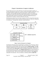
Consider a four input AND gate. The output function is described as an easy generalization 

of the two input AND gate; the output is 1 (True) if and only if all of the inputs are 1, 

otherwise the output is 0. One can synthesize a four-input AND gate from three two-input 

AND gates or easily convert a four-input AND gate into a two-input AND gate. The student 

should realize that each figure below represents only one of several good implementations. 

Figure: Three 2-Input AND Gates Make a 4-Input AND Gate 

Figure: Another Way to Configure Three 2-Input AND Gates as a 4-Input AND Gate 

Figure: Two Ways to Configure a 4-Input AND Gate as a 2-Input AND Gate 

Here is the general rule for N-Input AND gates and N-Input OR gates. 

AND Output is 0 if any input is 0. Output is 1 only if all inputs are 1. 

OR Output is 1 if any input is 1. Output is 0 only if all inputs are 0. 

XOR For N > 2, N-input XOR gates are not useful and will be avoided. 




“Derived Gates” 

We now show 2 gates that may be considered as derived from the above: NAND and NOR. 

The NOR gate is the 

same as an OR gate 

followed by a NOT 

gate. 

The NAND gate is the 

same as an AND gate 

followed by a NOT 

gate. 

Electrical engineers may validly object that these two gates are not “derived” in the sense 

that they are less basic than the gates previously discussed. In fact, NAND gates are often 

used to make AND gates. As always, we are interested in the non-engineering approach and 

stay with our view: NOT, AND, and OR are basic. We shall ignore the XNOR gate and, if 

needed, implement its functionality by an XOR gate followed by a NOT gate. 

As an exercise in logic, we show that the NAND (Not AND) gate is fundamental in that it 

can be used to synthesize the AND, OR, and NOT gates. We begin with the basic NAND. 

The basic truth table for the NAND is given by 

X Y X•Y ( X • Y) 

0 0 0 1 

0 1 0 1 

1 0 0 1 

1 1 1 0 

From this truth table, we see that 0• 0 = 1 and 1• 1 = 0, so we conclude that X • X = X and 

immediately have the realization of the NAND gate as a NOT gate. 

Figure: A NAND Gate Used as a NOT Gate 

To synthesize an AND gate from a NAND gate, we just note that NOT NAND is the same as 

NOT NOT AND, which is the same as AND. In other words X • Y = X • Y, and we follow 

the NAND gate with the NOT gate, implemented from another NAND gate. 




Here is the AND gate as implemented from two NAND gates. 

Figure: Two NAND Gates to Make an AND Gate 

In order to implement an OR gate, we must make use of DeMorgan’s law. As stated above, 

DeMorgan’s law is usually given as ( X • Y) 

= X + Y . We use straightforward algebraic 

manipulation to arrive at a variant statement of DeMorgan’s law. 

X • Y = X + Y = X + Y 

Using this strange equality, a direct result of DeMorgan’s law, we have the OR circuit. 

Figure: Three NAND Gates Used to Make an OR Gate 

Circuits and Truth Tables 

We now address an obvious problem – how to relate circuits to Boolean expressions. The 

best way to do this is to work some examples. Here is the first one. 

Question: 

What are the truth table and the Boolean expressions that describe the following circuit? 




The method to get the answer is to label each gate and determine the output of each. The 

following diagram shows the gates as labeled and the output of each gate. 

The outputs of each gate are as follows: 

The output of gate 1 is (X + Y), 

The output of gate 2 is (Y ⊕ Z), 

The output of gate 3 is X’, 

The output of gate 4 is X’ + (Y ⊕ Z), and 

The output of gate 5 is (X + Y) ⊕ [X’ + (Y ⊕ Z)] 

We now produce the truth table for the function. 

X Y Z X + Y (Y ⊕ Z) X’ X’ + (Y ⊕ Z) (X + Y) ⊕ [X’+(Y ⊕ Z)] 

0 0 0 0 0 1 1 1 

0 0 10 0 1 1 1 1 

0 1 0 1 1 1 1 0 

0 1 1 1 0 1 1 0 

1 0 0 1 0 0 0 1 

1 0 1 1 1 0 1 0 

1 1 0 1 1 0 1 0 

1 1 1 1 0 0 0 1 

The above is the truth table for the function realized by the figure on the previous page. 

Lets give a simpler representation. 


0 0 0 1 

0 0 1 1 

0 1 0 0 

0 1 1 0 

1 0 0 1 

1 0 1 0 

1 1 0 0 

1 1 1 1 




We now produce both the SOP and POS representations of this function. For the SOP, we 

look at the four 1’s of the function; for the POS, we look at the four zeroes. 

SOP 

POS 

F(X, Y, Z) = X’•Y’•Z’ + X’•Y’•Z + X•Y’•Z’ + X•Y•Z 

0 0 0 0 0 1 1 0 0 1 1 1 

F(X, Y, Z) = (X + Y’ + Z) • (X + Y’ + Z’) • (X’ + Y + Z’) • (X’ + Y’ + Z) 

0 1 0 0 1 1 1 0 1 1 1 0 

To simplify in SOP, we write the function in a slightly more complex form. 

F(X, Y, Z) = X’•Y’•Z’ + X’•Y’•Z + X’•Y’•Z’ + X•Y’•Z’ + X•Y•Z 

= X’•Y’•(Z’ + Z) + (X + X’)•Y’•Z’ + X•Y•Z 

= X’•Y’ + Y’•Z’ + X•Y•Z 

To simplify in POS, we again write the function in a slightly bizarre form. 

F(X, Y, Z) = (X + Y’ + Z) • (X + Y’ + Z’) • (X’ + Y + Z’) 

• (X’ + Y’ + Z) • (X + Y’ + Z) 

= (X + Y’) • (X’ + Y + Z’)• (Y’ + Z) 

We close this discussion by presenting the canonical SOP and POS using another notation. 

We rewrite the truth table for F(X, Y, Z), adding row numbers. 


0 0 0 0 1 

1 0 0 1 1 

2 0 1 0 0 

3 0 1 1 0 

4 1 0 0 1 

5 1 0 1 0 

6 1 1 0 0 

7 1 1 1 1 

Noting the positions of the 1’s and 0’s in the truth table gives us our standard notation. 

F(X, Y, Z) = Σ(0, 1, 4, 7) 

F(X, Y, Z) = Π(2, 3, 5, 6) 

Question: 

What is the circuit that corresponds to the following two Boolean functions? 

The reader might note that the two are simply different representations of the same function. 

The answer here is just to draw the circuits. The general rule is simple. 

SOP One OR gate connecting the output of a number of AND gates. 

POS One AND gate connecting the output of a number of OR gates. 




Here is the circuit for F2(A, B, C). It can be simplified. 

Here is the circuit for G2(A, B, C). It can be simplified. 

The Non–Inverting Buffer 

We now investigate a number of circuit elements that do not directly implement Boolean 

functions. The first is the non–inverting buffer, which is denoted by the following symbol. 

Logically, a buffer does nothing. Electrically, the buffer serves as an amplifier converting a 

degraded signal into a more useable form; specifically it does the following. 

A logic 1 (voltage in the range 2.0 – 5.0 volts) will be output as 5.0 volts. 

A logic 0 (voltage in the range 0.0 – 0.8 volts) will be output as 0.0 volts. 

While one might consider this as an amplifier, it is better considered as a “voltage adjuster”. 

We shall see another use of this and similar circuits when we consider MSI (Medium Scale 

Integrated) circuits in a future chapter. 




More “Unusual” Circuits 

Up to this point, we have been mostly considering logic gates in their ability to implement 

the functions of Boolean algebra. We now turn our attention to a few circuits that depend as 

much on the electrical properties of the basic gates as the Boolean functions they implement. 

We begin with a fundamental property of all electronic gates, called “gate delay”. This 

property will become significant when we consider flip–flops. 

We begin with consideration of a simple NOT gate, with Y = X , as shown below. 

From the viewpoint of Boolean algebra, there is nothing special about this gate. It 

implements the Boolean NOT function; nothing else. From the viewpoint of actual 

electronic circuits, we have another issue. This issue, called “gate delay”, reflects the fact 

that the output of a gate does not change instantaneously when the input changes. The output 

always lags the input by an interval of time that is the gate delay. For standard TTL circuits, 

such as the 74LS04 that implements the NOT function, the gate delay is about ten 

nanoseconds; the output does not change until 10 nanoseconds after the input changes. 

In the next figure, we postulate a NOT gate with a gate delay of 10 nanoseconds with an 

input pulse of width 20 nanoseconds. Note that the output trails the input by the gate delay; 

in particular we have an interval of 10 nanoseconds (one gate delay) during which X = 1 and 

X = 1, and also an interval of 10 nanoseconds during which X = 0 and X = 0. This is not a 

fault of the circuit; it is just a well–understood physical reality. 

The table just below gives a list of gate delay times for some popular gates. The source of 

this is the web page http://www.cs.uiowa.edu/~jones/logicsim/man/node5.html 

Number Description Gate Delay in Nanoseconds 

74LS00 2–Input NAND 9.5 

74LS02 2–Input NOR 10.0 

74LS04 Inverter (NOT) 9.5 

74LS08 2–Input AND 9.5 

74LS32 2–Input OR 14.0 

74LS86 2–Input XOR 10.0 

We can see that there is some variation is the gate delay times for various basic logic gates, 

but that the numbers tend to be about 10.0 nanoseconds. In our discussions that follow we 

shall make the assumption that all logic gates display the same delay time, which we shall 

call a “gate delay”. While we should understand that this time value is about 10 

nanoseconds, we shall not rely on its precise value. 




There are a number of designs that call for introducing a fixed delay in signal propagation so 

that the signal does not reach its source too soon. This has to do with synchronization issues 

seen in asynchronous circuits. We shall not study these, but just note them. 

The most straightforward delay circuit is based on the Boolean identity. 

This simple Boolean identity leads to the delay circuit. 

The delay is shown in the timing diagram below, in which Z lags X by 20 nanoseconds. 

The rule for application of gate delays is stated simply below. 

The output of a gate is stable one gate delay after all of its inputs are stable. 

We should note that the delay circuit above is logically equivalent to the non–inverting buffer 

discussed just above. The non–inverting buffer is different in two major ways: its time delay 

is less, and it usually serves a different purpose in the design. 

It should be clear that the output of a gate changes one gate delay after any of its inputs 

change. To elaborate on this statement, let us consider an exclusive or (XOR) chip. The 

truth table for an XOR gate is shown in the following table. 

X Y X ⊕ Y 

0 0 0 

0 1 1 

1 0 1 

1 1 0 

We now examine a timing diagram for this circuit under the assumption that the inputs are 

initially both X = 0 and Y = 0. First X changes to 1 and some time later so does Y. 

Here is the circuit. 




Here is the timing diagram. 

Note that the output, Z, changes one gate delay after input X changes and again one gate 

delay after input Y changes. This unusual diagram is shown only to make the point that the 

output changes one gate delay after any change of input. In the more common cases, all 

inputs to a circuit change at about the same time, so that this issue does not arise. 

We now come to a very important circuit, one that seems to implement a very simple 

Boolean identity. Specifically, we know that for all Boolean variables X: 

Given the above identity, the output of the following circuit would be expected to be 

identically 0. Such a consideration does not account for gate delays. 

Suppose that input X goes high and stays high for some time, possibly a number of gate 

delays. The output Z is based on the fact that the output Y lags X by one gate delay. 

Suppose we are dealing with the typical value of 10 nanoseconds for a gate delay. 

At T = 10, the value of X changes. Neither Y nor Z changes. 

At T = 20, the values of each of Y and Z change. 

The value of Y reflects the value of X at T = 10, so Y becomes 0. 

The value of Z reflects the value of both X and Y at T = 10. 

At T = 10, we had both X = 1 and Y = 1, so Z becomes 1 at T = 20. 

At T = 30, the value of Z changes again to reflect the values of X and Y at T = 20. 

Z becomes 0. 

What we have in the above circuit is a design to produce a very short pulse, of time duration 

equal to one gate delay. This facility will become very useful when we begin to design 

edge–triggered flip–flops in a future chapter. 




Tri–State Buffers 

We have now seen all of the logic gates to be used in this course. There is one more gate 

type that needs to be examined – the tri-state buffer. We begin with the examination of a 

simple (non-inverting buffer) and comment on its function. We discuss two basic types: 

enabled–high and enabled–low. The circuit diagrams for these are shown below. 

The difference between these two circuits relates to how the circuits are enabled. Note that 

the enabled-low tri–state buffer shows the standard use of the NOT dot on input. 

The following figure shows two ways of implementing an Enabled–Low Tri-State buffer, 

one using an Enabled-High Tri-State with a NOT gate on the Enable line. The significance 

of the overbar on the Enable input is that the gate is active when the control is logic 0. 

Figure: Two Views of an Enabled-Low Tri-State Buffer 

A tri-state buffer acts as a simple buffer when it is enabled; it passes the input through while 

adjusting its voltage to be closer to the standard. When the tri-state buffer is not enabled, it 

acts as a break in the circuit or an open switch (if you understand the terminology). A gate 

may be enabled high (C = 1) or enabled low (C = 0). Consider an enabled–high tri-state. 

Figure: Circuits Equivalent to an Enabled Tri–State and a Disabled Tri-State 

When the enable signal is C = 1, the tri-state acts as a simple buffer and asserts its input as an 

output. When the enable signal is C = 0, the tri-state does not assert anything on the output. 

Another way to describe a tri–state buffer is to say that it is in a high-impedance state (often 

called a “high–Z state” by engineers who use the symbol “Z” for impedance) when it is not 

enabled. This is simply to say that it offers such a resistance to transmission of its input that 

for all practical purposed it does not assert anything on its output. 




The Third State 

The definition of this “third state” in a tri–state buffer is both obvious and subtle. Compare 

the two circuits in the figure below. One is a buffer; the other is a tri–state buffer. 

For the circuit on the left, either F = 0 (0 volts) or F = 1 (5 volts). There is no other option. 

For the circuit on the right, when C = 1 then F = A, and takes a value of either 0 volts or 5 

volts, depending on the value of the input. When C = 0, F is simply not defined. 

One of the better ways to understand the tri-state buffer is to consider the following circuit 

with two Boolean inputs A and B, one output F, and an enable signal C. 

Note that the two tri–state buffers are enabled differently, so that the top buffer is enabled if 

and only if the bottom buffer is not enabled, and vice versa. The design insures that at no 

time are both of the tri–state buffers enabled, so that there is no conflict of voltages. 

C = 0 Only the top buffer is enabled F = A 

C = 1 Only the bottom buffer is enabled F = B 

The reader will note that the above circuit is logically equivalent to the one that follows. 

Given only this simple example, one might reasonably question the utility of tri–state buffers. 

It appears that they offer a novel and complex solution to a simple problem. The real use of 

these buffers lies in placing additional devices on a common bus, a situation in which the use 

of larger OR gates might prove difficult. 

Before addressing the standard uses of the tri–state buffer, we must review some of the basics 

of direct current electricity: voltage, current, and resistance. 




Review of Basic Electronics 

A traditional presentation of this material might have begun with a review of the basic 

concepts of direct current electricity. Your author has elected to postpone that discussion 

until this point in the course, at which time it is needed. 

A Basic Circuit 

We begin our discussion with a simple example circuit – a flashlight (or “electric torch” as 

the Brits call it). This has three basic components: a battery, a switch, and a light bulb. For 

our purpose, the flashlight has two possible states: on and off. Here are two diagrams. 

Light is Off 

Light is On 

In the both figures, we see a light bulb connected to a battery via two wires and a switch. 

When the switch is open, it does not allow electricity to pass and the light is not illuminated. 

When the switch is closed, the electronic circuit is completed and the light is illuminated. 

The figure above uses a few of the following basic circuit elements. 

We now describe each of these elements and then return to our flashlight example. The first 

thing we should do is be purists and note the difference between a cell and a battery, although 

the distinction is quite irrelevant to this course. A cell is what one buys in the stores today 

and calls a battery; these come in various sizes, including AA, AAA, C, and D. Each of 

these cells is rated at 1.5 volts, due to a common technical basis for their manufacture. 

Strictly speaking, a battery is a collection of cells, so that a typical flashlight contains one 

battery that comprises two cells; usually AA, C, or D. An automobile battery is truly a 

battery, being built from a number of lead-acid cells. 

A light is a device that converts electronic current into visible light. This is not a surprise. 

A switch is a mechanical device that is either open (not allowing transmission of current) or 

closed (allowing the circuit to be completed). Note that it is the opposite of a door, which 

allows one to pass only when open. 




The Idea of Ground 

Consider the above circuit, which suggests a two-wire design: one wire from the battery to 

the switch and then to the light bulb, and another wire from the bulb directly to the battery. 

One should note that the circuit does not require two physical wires, only two distinct paths 

for conducting electricity. Consider the following possibility, in which the flashlight has a 

metallic case that also conducts electricity. 

Physical Connection 

Equivalent Circuit 

Consider the circuit at left, which shows the physical connection postulated. When the 

switch is open, no current flows. When the switch is closed, current flows from the battery 

through the switch and light bulb, to the metallic case of the flashlight, which serves as a 

return conduit to the battery. Even if the metallic case is not a very good conductor, there is 

much more of it and it will complete the circuit with no problem. 

In electrical terms, the case of the battery is considered as a common ground, so that the 

equivalent circuit is shown at right. Note the new symbol in this circuit – this is the ground 

element. One can consider all ground elements to be connected by a wire, thus completing 

the circuit. In early days of radio, the ground was the metallic case of the radio – an 

excellent conductor of electricity. Modern automobiles use the metallic body of the car itself 

as the ground. Although iron and steel are not excellent conductors of electricity, the sheer 

size of the car body allows for the electricity to flow easily. 

To conclude, the circuit at left will be our representation of a 

flashlight. The battery provides the electricity, which flows through 

the switch when the switch is closed, then through the light bulb, and 

finally to the ground through which it returns to the battery. 

As a convention, all switches in diagrams will be shown in the open 

position unless there is a good reason not to. 

The student should regard the above diagram as showing a switch which is not necessarily 

open, but which might be closed in order to allow the flow of electricity. The convention of 

drawing a switch in the open position is due to the fact that it is easier to spot in a diagram. 




Voltage, Current, and Resistance 

It is now time to become a bit more precise in our discussion of electricity. We need to 

introduce a number of basic terms, many of which are named by analogy to flowing water. 

The first term to define is current, usually denoted in equations by the symbol I. We all 

have an intuitive idea of what a current is. Imagine standing on the bank of a river and 

watching the water flow. The faster the flow of water, the greater the current; flows of water 

are often called currents. 

In the electrical terms, current is the flow of electrons, which are one of the basic building 

blocks of atoms. While electrons are not the only basic particles that have charge, and are 

not the only particle that can bear a current; they are the most common within the context of 

electronic digital computers. Were one interested in electro-chemistry he or she might be 

more interested in the flow of positively charged ions. 

All particles have one of three basic electronic charges: positive, negative, or neutral. Within 

an atom, the proton has the positive charge, the electron has the negative charge, and the 

neutron has no charge. In normal life, we do not see the interior of atoms, so our experience 

with charges relates to electrons and ions. A neutral atom is one that has the same number of 

protons as it has electrons. However, electrons can be quite mobile, so that an atom may gain 

or lose electrons and, as a result, have too many electrons (becoming a negative ion) or too 

few electrons (becoming a positive ion). For the purposes of this course, we watch only the 

electrons and ignore the ions. 

An electric charge, usually denoted by the symbol Q, is usually associated with a large 

number of electrons that are in excess of the number of positive ions available to balance 

them. The only way that an excess of electrons can be created is to move the electrons from 

one region to another – robbing one region of electrons in order to give them to another. 

This is exactly what a battery does – it is an electron “pump” that moves electrons from the 

positive terminal to the negative terminal. Absent any “pumping”, the electrons in the 

negative terminal would return to the positive region, which is deficient in electrons, and 

cause everything to become neutral. But the pumping action of the battery prevents that. 

Should one provide a conductive pathway between the positive and negative terminals of a 

battery, the electrons will flow along that pathway, forming an electronic current. 

To clarify the above description, we present the following diagram, which shows a battery, a 

light bulb, and a closed switch. We see that the flow of electrons within the battery is only a 

part of a larger, complete circuit. 




Materials are often classified by their abilities to conduct electricity. Here are two common 

types of materials. 

Conductor 

Insulator 

A conductor is a substance, such as copper or silver, through which 

electrons can flow fairly easily. 

An insulator is a substance, such as glass or wood, that offers 

significant resistance to the flow of electrons. In many of our 

circuit diagrams we assume that insulators do not transmit electricity 

at all, although they all do with some resistance. 

The voltage is amount of pressure in the voltage pump. It is quite 

similar to water pressure in that it is the pressure on the electrons that 

causes them to move through a conductor. Consider again our 

flashlight example. The battery provides a pressure on the electrons 

to cause them to flow through the circuit. When the switch is open, 

the flow is blocked and the electrons do not move. When the switch 

is closed, the electrons move in response to this pressure (voltage) 

and flow through the light bulb. The light bulb offers a specific 

resistance to these electrons; it heats up and glows. 

As mentioned above, different materials offer various abilities to transmit electric currents. 

We have a term that measures the degree to which a material opposes the flow of electrons; 

this is called resistance, denoted by R in most work. Conductors have low resistance (often 

approaching 0), while insulators have high resistance. In resistors, the opposition to the flow 

of electrons generates heat – this is the energy lost by the electrons as they flow through the 

resistor. In a light bulb, this heat causes the filament to become red hot and emit light. 

An open switch can be considered as a circuit element of extremely high resistance. 

Summary 

We have discussed four terms so far. We now should mention them again. 

Charge 

Current 

Voltage 

Resistance 

This refers to an unbalanced collection of electrons. The term used 

for denoting charge is Q. The unit of charge is a coulomb. 

This refers to the rate at which a charge flows through a conductor. 

The term used for denoting current is I. The unit of current is an ampere. 

This refers to a force on the electrons that causes them to move. This force 

can be due to a number of causes – electro-chemical reactions in batteries 

and changing magnetic fields in generators. The term used for denoting 

voltage is V or E (for Electromotive Force). The unit of current is a volt. 

This is a measure of the degree to which a substance opposes the flow of 

electrons. The term for resistance is R. The unit of resistance is an ohm. 




Ohm’s Law and the Power Law 

One way of stating Ohm’s law (named for Georg Simon Ohm, a German teacher who 

discovered the law in 1827) is verbally as follows. 

The current that flows through a circuit element is directly proportional to the 

voltage across the circuit element and inversely proportional to the resistance 

of that circuit element. 

What that says is that doubling the voltage across a circuit element doubles the current flow 

through the element, while doubling the resistance of the element halves the current. 

Let’s look again at our flashlight example, this time with the switch shown as closed. 

The chemistry of the battery is pushing electrons away 

from the positive terminal, denoted as “+” through the 

battery towards the negative terminal, denoted as “–“. 

This causes a voltage across the only resistive element in 

the circuit – the light bulb. This voltage placed across the light bulb causes current to flow 

through it. 

In algebraic terms, Ohm’s law is easily stated: E = I•R, where 

E is the voltage across the circuit element, 

I is the current through the circuit element, and 

R is the resistance of the circuit element. 

Suppose that the light bulb has a resistance of 240 ohms and has a voltage of 120 volts across 

it. Then we say E = I•R or 120 = I•240 to get I = 0.5 amperes. 

As noted above, an element resisting the flow of electrons absorbs energy from the flow it 

obstructs and must emit that energy in some other form. Power is the measure of the flow of 

energy. The power due to a resisting circuit element can easily be calculated. 

The power law is states as P = E•I, where 

P is the power emitted by the circuit element, measured in watts, 

E is the voltage across the circuit element, and 

I is the current through the circuit element. 

Thus a light bulb with a resistance of 240 ohms and a voltage of 120 volts across it has a 

current of 0.5 amperes and a power of 0.5 • 120 = 60 watts. 

There are a number of variants of the power law, based on substitutions from Ohm’s law. 

Here are the three variants commonly seen. 

P = E•I P = E 2 / R P = I 2 •R 

In our above example, we note that a voltage of 120 volts across a resistance of 60 ohms 

would produce a power of P = (120) 2 / 240 = 14400 / 240 = 60 watts, as expected. 

The alert student will notice that the above power examples were based on AC circuit 

elements, for which the idea of resistance and the associated power laws become more 

complex (literally). Except for a few cautionary notes, this course will completely ignore the 

complexities of alternating current circuits. 




Resistors in Series 

There are very many interesting combinations of resistors found 

in circuits, but here we focus on only one – resistors in series; 

that is one resistor placed after another. In this figure, we 

introduce the symbol for a resistor. 

Consider the circuit at right, with two resistors having 

resistances of R 1 and R 2 , respectively. One of the basic laws of 

electronics states that the resistance of the two in series is 

simply the sum: thus R = R 1 + R 2 . Let E be the voltage provided by the battery. Then the 

voltage across the pair of resistors is given by E, and the current through the circuit elements 

is given by Ohm’s law as I = E / (R1 + R 2 ). Note that we invoke another fundamental law 

that the current through the two circuit elements in series must be the same. 

Again applying Ohm’s law we can obtain the voltage drops across each of the two resistors. 

Let E 1 be the voltage drop across R 1 and E 2 be that across R 2 . Then 

E 1 = I•R 1 = R 1 •E / (R 1 + R 2 ), and 

E 2 = I•R 2 = R 2 •E / (R 1 + R 2 ). 

It should come as no surprise that E 1 + E 2 = R 1 •E / (R 1 + R 2 ) + R 2 •E / (R 1 + R 2 ) 

= (R 1 + R 2 )•E / (R 1 + R 2 ) = E. 

If, as is commonly done, we assign the ground state as having zero voltage, then the voltages 

at the two points in the circuit above are simple. 

1) At point 1, the voltage is E, the full voltage of the battery. 

2) At point 2, the voltage is E 2 = I•R 2 = R 2 •E / (R 1 + R 2 ). 

Before we present the significance of the above circuit, consider two special cases. 

In the circuit at left, the second resistor is replaced by a conductor having zero resistance. 

The voltage at point 2 is then E 2 = 0•E / (R 1 + 0) = 0. As point 2 is directly connected to 

ground, we would expect it to be at zero voltage. 

Suppose that R 2 is much bigger than R 1 . Let R 1 = R and R 2 = 1000•R. We calculate the 

voltage at point 2 as E 2 = R 2 •E / (R 1 + R 2 ) = 1000•R•E / (R + 1000•R) = 1000•E/1001, or 

approximately E 2 = (1 – 1/1000)•E = 0.999•E. Point 2 is essentially at full voltage. 




Putting a Resistor and Switch in Series 

We now consider an important circuit that is related to the above circuit. In this circuit the 

second resistor, R 2 , is replaced by a switch that can be either open or closed. 

The Circuit Switch Closed Switch Open 

The circuit of interest is shown in the figure at left. What we want to know is the voltage at 

point 2 in the case that the switch is closed and in the case that the switch is open. In both 

cases the voltage at point 1 is the full voltage of the battery. 

When the switch is closed, it becomes a resistor with no resistance; hence R 2 = 0. As we 

noted above, this causes the voltage at point 2 to be equal to zero. 

When the switch is open, it becomes equivalent to a very large resistor. Some say that the 

resistance of an open switch is infinite, as there is no path for the current to flow. For our 

purposes, it suffices to use the more precise idea that the resistance is very big, at least 1000 

times the resistance of the first resistor, R 1 . The voltage at point 2 is the full battery voltage. 

Here is a version of the circuit as we shall use it later. 

Before we present our circuit, we introduce a notation used in 

drawing two wires that appear to cross. If a big dot is used at 

the crossing, the two wires are connected. If there is a gap, as in 

the right figure, then the wires do not connect. 

In this circuit, there are four switches attached to the wire. The voltage is monitored by 

another circuit that is not important at this time. If all four switches are open, then the 

voltage monitor registers full voltage. If one or more of the switches is closed, the monitor 

registers zero voltage. This is the best way to monitor a set of switches. 




Back to Tri–State Buffers 

We use the above verbiage to present a new view of tri–state buffers. Consider the following 

two circuits, which have been used previously in this chapter. Suppose that the battery is 

rated at five volts. In the circuit at left, point A is at 5 volts and point B is at 0 volts. In the 

circuit at right, point B is clearly at 0 volts, but the status of point A is less clear. 

What is obvious about the circuit at right is that there is no current flowing through it and no 

power being emitted by the light bulb. For this reason, we often say that point A is at 0 volts, 

but it is better to say that there is no specified voltage at that point. This is equivalent to the 

third state of a tri–state buffer; the open switch is not asserting anything at point A. 

Perhaps the major difference between the two circuits is that we can add another battery to 

the circuit at right and define a different voltage at point A. As long as the switch remains 

open, we have no conflict. Were the switch to be closed, we would have two circuits trying 

to force a voltage at point A. This could lead to a conflict. 

Device Polling 

Here is a more common use of tri–state buffers. Suppose a number of devices, each of which 

can signal a central voltage monitor by asserting logic zero (0 volts) on a line. Recalling that 

a logic AND outputs 0 if any of its inputs are 0, we could implement the circuit as follows. 

Suppose we wanted to add another device. This would require pulling the 4–input AND gate 

and replacing it with a 5–input AND gate. Continual addition of devices would push the 

technology beyond the number of inputs a normal gate will support. 

The tri–state solution avoids these problems. This circuit repeats the one shown above with 

the switches replaced by tri–state buffers, which should be viewed as switches. 

One should note that additional devices can be added to this circuit merely by attaching 

another tri–state switch. The only limit to extensibility of this circuit arises from timing 

considerations of signal propagation along the shared line. 




Solved Problems 

We now present a series of solved problems from previous homework and exams. 

PROBLEM 

Draw a circuit diagram to show how to implement 

a) a three-input AND gate using only two-input AND gates. 

b) a four-input AND gate using only three-input AND gates. 

c) a three-input AND gate using only one four-input AND gate. 

One set of solutions is shown below. There are others. 

PROBLEM 

If A = 0, B = 1, C = 0, and D = 1, find the value of F for each of the following. 

a) F = A•B’ + C 

Answer: F = 0•1’ + 0 = 0•0 + 0 = 0 

b) F = A•B’ + C’•D + C•D 

Answer: F = 0•1’ + 0’•1 + 0•1 = 0•0 + 1•1 + 0•1 = 0 + 1 + 0 = 1 

c) F = (A + B’)•(C’ + A)•(A + B•C) 

Answer: F = (0 + 1’)•(0’ + 0)•(0 + 1•0) = (0 + 0)•(1 + 0)•(0 + 0) = 0•1•0 = 0 




PROBLEM 

Draw a truth table for each of the following 

a) Q = X•Y’ + X’•Z’ + X•Y•Z 

Here is the truth table 

X Y Z X’ Y’ Z’ X•Y’ X’•Z’ X•Y•Z Q 

0 0 0 1 1 1 0 1 0 1 

0 0 1 1 1 0 0 0 0 0 

0 1 0 1 0 1 0 1 0 1 

0 1 1 1 0 0 0 0 0 0 

1 0 0 0 1 1 1 0 0 1 

1 0 1 0 1 0 1 0 0 1 

1 1 0 0 0 1 0 0 0 0 

1 1 1 0 0 0 0 0 1 1 

b) Q = (X’ + Y)•(X’ + Z’)•(X + Z) 

Here is the truth table. 

X Y Z X’ Z’ (X’ + Y) (X’ + Z’) (X + Z) Q 

0 0 0 1 1 1 1 0 0 

0 0 1 1 0 1 1 1 1 

0 1 0 1 1 1 1 0 0 

0 1 1 1 0 1 1 1 1 

1 0 0 0 1 0 1 1 0 

1 0 1 0 0 0 0 1 0 

1 1 0 0 1 1 1 1 1 

1 1 1 0 0 1 0 1 0 

PROBLEM 

Describe the form for each of the following Boolean expressions. 

a) F(X, Y, Z) = X•Y’ + Y•Z’ + Z’•Y’ 

b) F(A, B, C, D) = (A + B’ + C’)•(A’ + C’ + D)•(A’ + C’) 

c) F(P, Q, R) = P•Q’ + Q•R’•(P + Q’) + (R’ + Q’) 

d) F(A, B, C) = (A + B + C’)•(A’ + B’ + C’)•(A’ + B + C’) 

e) F(A, B, C, D) = A•B•C’•D + A•B’•C’•D’ + A’•B’•C•D 

f) F(A, B, C) = (A + B’ + C)•(A + B’)•(A + B + C’) 




Solutions 

a) F(X, Y, Z) = X•Y’ + Y•Z’ + Z’•Y’ 

This is a normal SOP expression. The last product term could easily be written as Y’•Z’ 

and normally would be so written; however, the order of literals is not important in 

determining the form of an expression. The two terms Y’•Z’ and Y•Z’ both contain the 

variables Y and Z, but the literals are different so we have no included terms. 

Note that since Y’ + Y ≡ 1, we can simplify this to F(X, Y, Z) = X•Y’ + (Y’ + Y)•Z’, 

which becomes F(X, Y, Z) = X•Y’ + Z’. 

b) F(A, B, C, D) = (A + B’ + C’)•(A’ + C’ + D)•(A’ + C’) 

This is obviously a POS expression. It is also obvious that it is not a canonical form. The 

first term by itself shows that the form is not canonical; it lacks a literal for the variable D. 

We now note the second and third terms and see that the third term is included in the second 

term, so the form is not normal. The answer is POS form, not a normal form. 

As an exercise, we convert the expression (A + B’ + C)•(A’ + C’ + D)•(A’ + C’) into a 

normal form. We use a form of the absorption theorem X•(X + Y) = X for any X and Y. We 

see the truth of this theorem by considering two cases X = 0 and X = 1. For X = 0, the 

identity becomes 0•(0 + Y) = 0 and for X = 1 it becomes 1•(1 + Y) = 1, both true. We now 

consider the above with X = A’ + C’ and Y = D; thus (A’ + C’ + D)•(A’ + C’) = (A’ + C’) 

and we obtain F(A, B, C, D) = (A + B’ + C)•(A’ + C’). 

c) F(P, Q, R) = P•Q’ + Q•R’•(P + Q’) + (R’ + Q’) 

This is not either a POS form or a SOP form, although many students wish to label it a SOP 

form as it can be easily converted to SOP. Answer: Not in any normal form. 

Again as an exercise, we convert the expression P•Q’ + Q•R’•(P + Q’) + (R’ + Q’) to a 

normal form. 

F(P, Q, R) = P•Q’ + Q•R’•(P + Q’) + (R’ + Q’) 

= P•Q’ + P•Q•R’ + Q•Q’•R’ + R’ + Q’ 

= P•Q’ + P•Q•R’ + R’ + Q’ as Q•Q’•R’ = 0 for any value of Q 

= P•Q’ + Q’ + P•Q•R’ + R’ 

= (P + 1)•Q’ + (P•Q + 1)•R’ 

= Q’ + R’ as 1 + X = 1 for any literal X. 

Our simplification has dropped all but the last term in the original expression. 

d) F(A, B, C) = (A + B + C’)•(A’ + B’ + C’)•(A’ + B + C’) 

This is a canonical POS expression. We note that it can be simplified , noting that 

(X + Y)•(X + Y’) = X for any X and Y (for Y = 0, the left hand side of the identity is 

(X + 0)•(X + 1) = X; for Y = 1 it is (X + 1)•(X + 0) = X). To simplify, let X = A’ + C’ and 

Y = B. So (A’ + B’ + C’)•(A’ + B + C’) = (A’ + C’) and F = (A + B + C’)•(A’ + C’). 




e) F(A, B, C, D) = A•B•C’•D + A•B’•C’•D’ + A’•B’•C•D 

This is a canonical SOP expression. Every term is a product term. The expression 

is the logical OR of the terms, so we have a SOP expression. There are no included 

terms – the first contains literal A, while the other two do not and the second contains 

a C’ while the third does not. Thus the expression is a normal SOP. As each of the 

three terms has a literal for each of the four variables, this is a canonical SOP. 

f) F(A, B, C) = (A + B’ + C)•(A + B’)•(A + B + C’) 

This is obviously some sort of POS expression. Each term is a sum term and the 

expression is the logical OR of the terms. However, the second term (A + B’) is 

contained in the first expression (A + B’ + C). 

The expression is Product of Sums, but not normal. 

We use the equality X•(X + Y) = X to simplify the expression. First we prove the 

equality. For X = 0, we have 

LHS = 0•(0 + Y) = 0•(Y) = 0 

RHS = 0 

For X = 1, we have 

LHS = 1•(1 + Y) = 1•(1) = 1 

RHS = 1 

If we let X = (A + B’) and Y = C, we have an expression of the form 

(X + Y)•X•(A + B + C’) = X•(A + B + C’) = (A + B’)•(A + B + C’). 

This second expression is in Normal Product of Sums. The first term lacks a 

literal for the variable C, so the expression is not in canonical form. 

EXTRA QUESTION: What is the form of the expression F(P, Q, R) = Q’ + R’? 

There are two answers – either Normal POS or Normal SOP. 

It is clear that the expression is not canonical, as both terms lack a P. For an expression to be 

canonical, each variable must appear in every term, in either the complemented or noncomplemented 

form. 

SOP: Each of the two terms Q’ and R’ can be viewed as a product term. Admittedly, we 

normally think of two or more literals (such as Q•R) when we say “product term”, 

but a product term can have one literal. This is the logical OR of two product terms. 

POS: Each of the two terms Q’ and R’ is a literal. The term (Q’ + R’) is a good sum term. 

Here we have the product of one sum term, so POS. 

As a follow-on, we note the forms of the expression F(Q, R) = Q’ + R’. The answer now is 

either canonical POS or normal SOP, depending on how one wants to read it. As a canonical 

POS, the expression has one sum term that contains a literal for each of Q and R. As a 

normal SOP, we note that the first product term lacks a literal for R and the second product 

term lacks a literal for Q, so the expression as an SOP is not canonical. However, it is the 

sum of two product terms, with no inclusion. 




PROBLEM 

Prove the following equality for Boolean variables X and Y by any valid means you find 

convenient. Show all of your work. 

X ⊕ Y = X • Y + X • Y 

A truth table provides the best proof. The functions 

X ⊕ Y and X • Y + X•Y match exactly. 

X Y X⊕Y X ⊕ Y X • Y X•Y X • Y + X•Y Match? 

0 0 0 1 1 0 1 Yes 

0 1 1 0 0 0 0 Yes 

1 0 1 0 0 0 0 Yes 

1 1 0 1 0 1 1 Yes 

PROBLEM 

Generate a truth-table for F(X, Y, Z) = 

X • Y • Z + X • Y • Z + X • Y • Z 

ANSWER: We first write this as 

negated. We then create the truth table. 

to emphasize the blocks that are 

X Y Z Y•Z X•Y•Z X•(Y•Z)’ (X•Y•Z)’ F(X, Y, Z) 

0 0 0 0 0 0 1 1 

0 0 1 0 0 0 1 1 

0 1 0 0 0 0 1 1 

0 1 1 1 0 0 1 1 

1 0 0 0 0 1 1 1 

1 0 1 0 0 1 1 1 

1 1 0 0 0 1 1 1 

1 1 1 1 1 0 0 1 

Notes: Generate the term in two parts. For X = 0, the term is 0. 

For X = 1, the term is (Y•Z)’, the opposite of Y•Z. 

PROBLEM 

Let A = X•Y•Z. This is of the form A + B + A’ = A + A’ + something = 1. 

Produce a truth table for F(X, Y, Z) = ( X + Y) • ( X + Z) • ( X + Z) 




ANSWER: This is most easily cracked with algebra, noting that 

we simply produce the truth table for (X + Y) • Z. 

X Y Z (X + Y) (X + Y) • Z 

0 0 0 0 0 

0 0 1 0 0 

0 1 0 1 0 

0 1 1 1 1 

1 0 0 1 0 

1 0 1 1 1 

1 1 0 1 0 

1 1 1 1 1 

PROBLEM 

Write the expression for the complement of F, if F = 

ANSWER: First we solve a problem with the same form. If F(A, B, C) = A + B + C, then 

what is the complement of F? We apply DeMorgan’s law twice to get the result. 

Then 

So 

and 

NOTES: 

Please remember that A + B • C + D is not the same as the expression 

(A + B) • (C + D). By definition A + B • C + D = A + (B • C) + D. 

One could also write (A + B) • (C + D) as (A + B)(C + D). 

The next two problems refer to the following truth table. 


0 0 0 1 

0 0 1 0 

0 1 0 0 

0 1 1 1 

1 0 0 0 

1 0 1 0 

1 1 0 1 

1 1 1 0 




PROBLEM 

Represent the above truth table as a Boolean expression in SOP form. 

ANSWER: One can write this expression as F(X, Y, Z) = Σ(0, 3, 6), as rows 0, 3, and 6 ar 

the rows with F = 1. To write the SOP, we focus on these rows. 

The term for row 0 is X’•Y’•Z’, as X = 0, Y = 0, and Z = 0 for the entry in that row. 

The term for row 3 is X’•Y•Z, as X = 0, Y = 1, and Z = 1 for the entry in that row. 

The term for row 6 is X•Y•Z’, as X = 1, Y = 1, and Z = 0 for the entry in that row. 

The answer is F(X, Y, Z) = X’•Y’•Z’ + X’•Y•Z + X•Y•Z’. 

PROBLEM 

Represent the above truth table as a Boolean expression in POS form. 

ANSWER: One can also write the expression as F(X, Y, Z) = Π(1, 2, 4, 5, 7), as rows 

1, 2, 4, 5, and 7 are the rows with F = 0. To write the POS, we focus on these rows. 

The term for row 1 is (X + Y + Z’) as X = 0, Y = 0, and Z = 1 for that row. 

The term for row 2 is (X + Y’ + Z) as X = 0, Y = 1, and Z = 0 for that row. 

The term for row 4 is (X’ + Y + Z) as X = 1, Y = 0, and Z = 0 for that row. 

The term for row 5 is (X’ + Y + Z’) as X = 1, Y = 0, and Z = 1 for that row. 

The term for row 7 is (X’ + Y’ + Z’) as X = 1, Y = 1, and Z = 1 for that row. 

F(X, Y, Z) = (X + Y + Z’)•(X + Y’ + Z)•(X’ + Y + Z)•(X’ + Y + Z’)•(X’ + Y’ + Z’) 

This function can obviously be simplified. I attempt a Q-M procedure. 

Rows with one 1 0 0 1, 0 1 0, and 1 0 0 

Rows with two 1’s 1 0 1 

Rows with three 1’s 1 1 1 

Combine 0 0 1 and 1 0 1 to get – 0 1. Combine 1 0 0 and 1 0 1 to get 1 0 – 

Combine 1 0 1 and 1 1 1 to get 1 – 1 

The terms are now – 0 1, 0 1 0, 1 0 –, and 1 – 1. 

F(X, Y, Z) = (Y + Z’)•(X + Y’ + Z)•(X’ + Y)•(X’ + Z’) 




PROBLEMS FOR SOLUTION 

1. Using any proof method desired, prove that X • Y = X + Y for all X and Y. 

2. Produce the truth-table for the Boolean function 

G(A, B, C) = (A•B + C)•(A + B•C). 

The next few problems are based on the following truth table. 

A B C F(A, B, C) 

0 0 0 0 

0 0 1 1 

0 1 0 1 

0 1 1 0 

1 0 0 1 

1 0 1 1 

1 1 0 0 

1 1 1 1 

3. Produce the Σ-list and Π-list representations of this function. 

4. Represent this function in both canonical SOP and canonical POS form. 

5. Design a circuit using only AND, OR, and NOT gates to implement this function. 

The next few problems are based on the function G(A, B, C) = Π(2, 5). 

6. Write the Σ-list representation of this function. 

7. Represent this function in both canonical POS form and canonical SOP form. 

8. Design a circuit using only AND, OR, and NOT gates to implement this function. 

9. The notes show that the NAND gate is universal, in that one can use a NAND gate to 

make an AND gate, OR gate, and NOT gate. Show how to use a NOR gate to make 

an AND gate, OR gate, and NOT gate. Draw the circuit diagrams for these. 

10. Use two 2-input OR gates to make a 3-input OR gate. Show the design. 

11. Use a single 3-input OR gate to make a 2-input OR gate. Show the design.

Boolean Algebra and Some Combinational Circuits

You also want an ePaper? Increase the reach of your titles

Delete template?

Save as template?