MATLAB by Example - Department of Engineering
MATLAB by Example - Department of Engineering
MATLAB by Example - Department of Engineering

You also want an ePaper? Increase the reach of your titles
YUMPU automatically turns print PDFs into web optimized ePapers that Google loves.
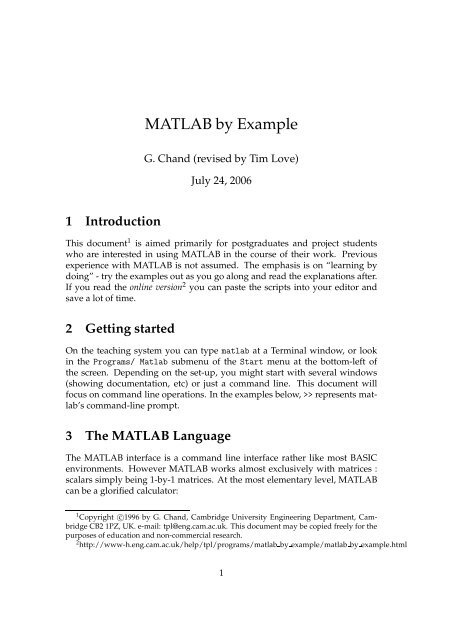
<strong>MATLAB</strong> <strong>by</strong> <strong>Example</strong><br />
G. Chand (revised <strong>by</strong> Tim Love)<br />
July 24, 2006<br />
1 Introduction<br />
This document 1 is aimed primarily for postgraduates and project students<br />
who are interested in using <strong>MATLAB</strong> in the course <strong>of</strong> their work. Previous<br />
experience with <strong>MATLAB</strong> is not assumed. The emphasis is on “learning <strong>by</strong><br />
doing” - try the examples out as you go along and read the explanations after.<br />
If you read the online version 2 you can paste the scripts into your editor and<br />
save a lot <strong>of</strong> time.<br />
2 Getting started<br />
On the teaching system you can type matlab at a Terminal window, or look<br />
in the Programs/ Matlab submenu <strong>of</strong> the Start menu at the bottom-left <strong>of</strong><br />
the screen. Depending on the set-up, you might start with several windows<br />
(showing documentation, etc) or just a command line. This document will<br />
focus on command line operations. In the examples below, >> represents matlab’s<br />
command-line prompt.<br />
3 The <strong>MATLAB</strong> Language<br />
The <strong>MATLAB</strong> interface is a command line interface rather like most BASIC<br />
environments. However <strong>MATLAB</strong> works almost exclusively with matrices :<br />
scalars simply being 1-<strong>by</strong>-1 matrices. At the most elementary level, <strong>MATLAB</strong><br />
can be a glorified calculator:<br />
1 Copyright c○1996 <strong>by</strong> G. Chand, Cambridge University <strong>Engineering</strong> <strong>Department</strong>, Cambridge<br />
CB2 1PZ, UK. e-mail: tpl@eng.cam.ac.uk. This document may be copied freely for the<br />
purposes <strong>of</strong> education and non-commercial research.<br />
2 http://www-h.eng.cam.ac.uk/help/tpl/programs/matlab <strong>by</strong> example/matlab <strong>by</strong> example.html<br />
1
fred=6*7<br />
>> FRED=fred*j;<br />
>> exp(pi*FRED/42)<br />
>> whos<br />
<strong>MATLAB</strong> is case sensitive so that the two variables fred and FRED are different.<br />
The result <strong>of</strong> an expression is printed out unless you terminate the<br />
statement <strong>by</strong> a ‘ ;’. j (and i) represent the square root <strong>of</strong> -1 unless you define<br />
them otherwise. who lists the current environment variable names and whos<br />
provides details such as size, total number <strong>of</strong> elements and type. Note that the<br />
variable ans is set if you type a statement without an ‘ =’ sign.<br />
4 Matrices<br />
So far you have operated on scalars. <strong>MATLAB</strong> provides comprehensive matrix<br />
operations. Type the following in and look at the results:<br />
>> a=[3 2 -1<br />
0 3 2<br />
1 -3 4]<br />
>> b=[2,-2,3 ; 1,1,0 ; 3,2,1]<br />
>> b(1,2)<br />
>> a*b<br />
>> det(a)<br />
>> inv(b)<br />
>> (a*b)’-b’*a’<br />
>> sin(b)<br />
The above shows two ways <strong>of</strong> specifying a matrix. The commas in the<br />
specification <strong>of</strong> b can be replaced with spaces. Square brackets refer to vectors<br />
and round brackets are used to refer to elements within a matrix so that b(x,y)<br />
will return the value <strong>of</strong> the element at row x and column y. Matrix indices<br />
must be greater than or equal to 1. det and inv return the determinant and<br />
inverse <strong>of</strong> a matrix respectively. The ’ performs the transpose <strong>of</strong> a matrix. It<br />
also complex conjugates the elements. Use .’ if you only want to transpose a<br />
complex matrix.<br />
The * operation is interpreted as a matrix multiply. This can be overridden<br />
<strong>by</strong> using .* which operates on corresponding entries. Try these :<br />
2
c=a.*b<br />
>> d=a./b<br />
>> e=a.^b<br />
For example c(1,1) is a(1,1)*b(1,1). The Inf entry in d is a result <strong>of</strong><br />
dividing 2 <strong>by</strong> 0. The elements in e are the results <strong>of</strong> raising the elements in a<br />
to the power <strong>of</strong> the elements in b. Matrices can be built up from other matrices:<br />
>> big=[ones(3), zeros(3); a , eye(3)]<br />
big is a 6-<strong>by</strong>-6 matrix consisting <strong>of</strong> a 3-<strong>by</strong>-3 matrix <strong>of</strong> 1’s, a 3-<strong>by</strong>-3 matrix <strong>of</strong><br />
0’s, matrix a and the 3-<strong>by</strong>-3 identity matrix.<br />
It is possible to extract parts <strong>of</strong> a matrix <strong>by</strong> use <strong>of</strong> the colon:<br />
>> big(4:6,1:3)<br />
This returns rows 4 to 6 and columns 1 to 3 <strong>of</strong> matrix big. This should result<br />
in matrix a. A colon on its own specifies all rows or columns:<br />
>> big(4,:)<br />
>> big(:,:)<br />
>> big(:,[1,6])<br />
>> big(3:5,[1,4:6])<br />
The last two examples show how vectors can be used to specify which noncontiguous<br />
rows and columns to use. For example the last example should<br />
return columns 1, 4, 5 and 6 <strong>of</strong> rows 3, 4 and 5.<br />
5 Constructs<br />
<strong>MATLAB</strong> provides the for, while and if constructs. <strong>MATLAB</strong> will wait for<br />
you to type the end statement before it executes the construct.<br />
>> y=[];<br />
>> for x=0.5:0.5:5<br />
y=[y,2*x];<br />
end<br />
3
y<br />
>> n=3;<br />
>> while(n ~= 0)<br />
n=n-1<br />
end<br />
>> if(n < 0)<br />
-n<br />
elseif (n == 0)<br />
n=365<br />
else<br />
n<br />
end<br />
The three numbers in the for statement specify start, step and end values for<br />
the loop. Note that you can print a variable’s value out <strong>by</strong> mentioning it’s<br />
name alone on the line. ~= means ‘not equal to’ and == means ‘equivalent to’.<br />
6 Help<br />
The help command returns information on <strong>MATLAB</strong> features:<br />
>> help sin<br />
>> help colon<br />
>> help if<br />
help without any arguments returns a list <strong>of</strong> <strong>MATLAB</strong> topics. You can also<br />
search for functions which are likely to perform a particular task <strong>by</strong> using<br />
lookfor:<br />
>> lookfor gradient<br />
The <strong>MATLAB</strong> hypertext reference documentation can be accessed <strong>by</strong> typing<br />
doc.<br />
7 Programs<br />
Rather than entering text at the prompt, <strong>MATLAB</strong> can get its commands from<br />
a .m file. If you type edit prog1, Matlab will start an editor for you. Type in<br />
the following and save it.<br />
4
for x=1:10<br />
y(x)=x^2+x;<br />
end<br />
y<br />
The step term in the for statement defaults to 1 when omitted. Back inside<br />
<strong>MATLAB</strong> run the script <strong>by</strong> typing:<br />
>> prog1<br />
which should result in vector y being displayed numerically. Typing<br />
>> plot(y)<br />
>> grid<br />
should bring up a figure displaying y(x) against x on a grid. Like many matlab<br />
routines plot can take a variable number <strong>of</strong> arguments. With just one<br />
argument (as here) the argument is taken as a vector <strong>of</strong> y values, the x values<br />
defaulting to 1,2,..., Note the effect <strong>of</strong> resizing the figure window.<br />
The Teaching System is set up so that if you have a directory called matlab<br />
in your home directory, then .m scripts there will be run irrespective <strong>of</strong> which<br />
directory you were in when you started matlab.<br />
8 Applications<br />
8.1 Graphical solutions<br />
<strong>MATLAB</strong> can be used to plot 1-d functions. Consider the following problem:<br />
Find to 3 d.p. the root nearest 7.0 <strong>of</strong> the equation 4x 3 + 2x 2 − 200x − 50 = 0<br />
<strong>MATLAB</strong> can be used to do this <strong>by</strong> creating file eqn.m in your matlab directory:<br />
function [y] = eqn(x)<br />
% User defined polynomial function<br />
[rows,cols] = size(x);<br />
for index=1:cols<br />
5
y(index) = 4*x(index)^3+2*x(index)^2-200*x(index)-50;<br />
end<br />
The first line defines ‘eqn’ as a function – a script that can take arguments.<br />
The square brackets enclose the comma separated output variable(s) and the<br />
round brackets enclose the comma separated input variable(s) - so in this case<br />
there’s one input and one output. The % in the second line means that the rest<br />
<strong>of</strong> the line is a comment. However, as the comment comes immediately after<br />
the function definition, it is displayed if you type :<br />
>> help eqn<br />
The function anticipates x being a row vector so that size(x) is used to find<br />
out how many rows and columns there are in x. You can check that the root is<br />
close to 7.0 <strong>by</strong> typing:<br />
>> eqn([6.0:0.5:8.0])<br />
Note that eqn requires an argument to run which is the vector [6.0 6.5 7.0 7.5<br />
8.0].<br />
The for loop in <strong>MATLAB</strong> should be avoided if possible as it has a large<br />
overhead. eqn.m can be made more compact using the . notation. Delete the<br />
lines in eqn.m and replace them with:<br />
function [y] = eqn(x)<br />
% COMPACT user defined polynomial function<br />
y=4*x.^3+2*x.^2-200*x-50;<br />
Now if you type ‘ eqn([6.0:0.5:8.0])’ it should execute your compact eqn.m<br />
file.<br />
Now edit and save ploteqn.m in your matlab directory:<br />
x est = 7.0;<br />
delta = 0.1;<br />
while(delta > 1.0e-4)<br />
x=x est-delta:delta/10:x est+delta;<br />
fplot(’eqn’,[min(x) max(x)]);<br />
grid;<br />
6
disp(’mark position <strong>of</strong> root with mouse button’)<br />
[x est,y est] = ginput(1)<br />
delta = delta/10;<br />
end<br />
This uses the function fplot to plot the equation specified <strong>by</strong> function eqn.m<br />
between the limits specified. ginput with an argument <strong>of</strong> 1 returns the x- and<br />
y-coordinates <strong>of</strong> the point you have clicked on. The routine should zoom into<br />
the root with your help. To find the actual root try matlab’s solve routine:<br />
>> poly = [4 2 -200 -50];<br />
>> format long<br />
>> roots(poly)<br />
>> format<br />
which will print all the roots <strong>of</strong> the polynomial : 4x 3 + 2x 2 − 200x − 50 = 0 in<br />
a 15 digit format. format on its own returns to the 5 digit default format.<br />
8.2 Plotting in 2D<br />
<strong>MATLAB</strong> can be used to plot 2-d functions e.g. 5x 2 + 3y 2 :<br />
>> [x,y]=meshgrid(-1:0.1:1,-1:0.1:1);<br />
>> z=5*x.^2+3*y.^2;<br />
>> contour(x,y,z);<br />
>> prism;<br />
>> mesh(x,y,z)<br />
>> surf(x,y,z)<br />
>> view([10 30])<br />
>> view([0 90])<br />
The meshgrid function creates a ‘mesh grid’ <strong>of</strong> x and y values ranging from -1<br />
to 1 in steps <strong>of</strong> 0.1. If you look at x and y you might get a better idea <strong>of</strong> how z<br />
(a 2D array) is created. The mesh function displays z as a wire mesh and surf<br />
displays it as a facetted surface. prism simply changes the set <strong>of</strong> colours in the<br />
contour plot. view changes the horizontal rotation and vertical elevation <strong>of</strong> the<br />
3D plot. The z values can be processed and redisplayed<br />
>> mnz=min(min(z));<br />
>> mxz=max(max(z));<br />
7
z=255*(z-mnz)/(mxz-mnz);<br />
>> image(z);<br />
>> colormap(gray);<br />
image takes interprets a matrix as a <strong>by</strong>te image. For other colormaps try help<br />
color.<br />
9 Advanced plotting<br />
Consider the following problem:<br />
Display the 2D Fourier transform intensity <strong>of</strong> a square slit.<br />
(The 2D Fourier transform intensity is the diffraction pattern). Enter the following<br />
into square_fft.m :<br />
echo on<br />
colormap(hsv);<br />
x=zeros(32);<br />
x(13:20,13:20)=ones(8);<br />
mesh(x)<br />
pause % strike a key<br />
y=fft2(x);<br />
z=real(sqrt(y.^2));<br />
mesh(z)<br />
pause<br />
w=fftshift(z);<br />
surf(w)<br />
pause<br />
contour(log(w+1))<br />
prism<br />
pause<br />
plot(w(1:32,14:16))<br />
title(’fft’)<br />
xlabel(’frequency’)<br />
ylabel(’modulus’)<br />
grid<br />
echo <strong>of</strong>f<br />
8
The echo function displays the operation being currently executed. The program<br />
creates a 8-<strong>by</strong>-8 square on a 32x32 background and performs a 2D FFT<br />
on it. The intensity <strong>of</strong> the FFT (the real part <strong>of</strong> y) is stored in z and the D.C.<br />
term is moved to the centre in w. Note that the plot command when given a 3<br />
<strong>by</strong> 32 array displays 3 curves <strong>of</strong> 32 points each.<br />
10 Input and output<br />
Data can be be transferred to and from <strong>MATLAB</strong> in four ways:<br />
1. Into <strong>MATLAB</strong> <strong>by</strong> running a .m file<br />
2. Loading and saving .mat files<br />
3. Loading and saving data files<br />
4. Using specialised file I/O commands in <strong>MATLAB</strong><br />
The first <strong>of</strong> this involves creating a .m file which contains matrix specifications<br />
e.g. if mydata.m contains:<br />
data = [1 1;2 4;3 9;4 16;5 25;6 36];<br />
Then typing:<br />
>> mydata<br />
will enter the matrix data into <strong>MATLAB</strong>. Plot the results (using the cursor controls,<br />
it is possible to edit previous lines):<br />
>> handout length = data(:,1);<br />
>> boredom = data(:,2);<br />
>> plot(handout length,boredom);<br />
>> plot(handout length,boredom,’*’);<br />
>> plot(handout length,boredom,’g.’,handout length,boredom,’ro’);<br />
A .mat file can be created <strong>by</strong> a save command in a <strong>MATLAB</strong> session (see below).<br />
Data can be output into ASCII (human readable) or non-ASCII form:<br />
9
save results.dat handout length boredom -ascii<br />
>> save banana.peel handout length boredom<br />
The first <strong>of</strong> these saves the named matrices in file results.dat (in your current<br />
directory) in ASCII form one after another. The second saves the matrices<br />
in file banana.peel in non-ASCII form with additional information such as the<br />
name <strong>of</strong> the matrices saved. Both these files can be loaded into <strong>MATLAB</strong> using<br />
load :<br />
>> clear<br />
>> load banana.peel -mat<br />
>> whos<br />
>> clear<br />
>> load results.dat<br />
>> results<br />
>> apple=reshape(results,6,2)<br />
The clear command clears all variables in <strong>MATLAB</strong>. The mat option in load<br />
interprets the file as a non-ASCII file. reshape allows you to change the shape<br />
<strong>of</strong> a matrix. Using save on its own saves the current workspace in matlab.mat<br />
and load on its own can retrieve it.<br />
<strong>MATLAB</strong> has file I/O commands (much like those <strong>of</strong> C) which allow you<br />
to read many data file formats into it. Create file alpha.dat with ABCD as its<br />
only contents. Then:<br />
>> fid=fopen(’alpha.dat’,’r’);<br />
>> a=fread(fid,’uchar’,0)+4;<br />
>> fclose(fid);<br />
>> fid=fopen(’beta.dat’,’w’);<br />
>> fwrite(fid,a,’uchar’);<br />
>> fclose(fid);<br />
>> !cat beta.dat<br />
Here, alpha.dat is opened for reading and a is filled with unsigned character<br />
versions <strong>of</strong> the data in the file with 4 added on to their value. beta.dat is then<br />
opened for writing and the contents <strong>of</strong> a are written as unsigned characters to<br />
it. Finally the contents <strong>of</strong> this file are displayed <strong>by</strong> calling the Unix command<br />
cat (the ’!’ command escapes from matlab into unix).<br />
10
help fopen<br />
>> help fread<br />
will provide more information on this <strong>MATLAB</strong> facility.<br />
11 Common problems<br />
If you need save data in files data1.mat data2.mat etc. use eval in a .m file e.g.<br />
for x=1:5<br />
results=x;<br />
operation=[’save ’,’data’,num2str(x),’ results’]<br />
eval(operation)<br />
end<br />
The first time this loop is run, ’save data1 results’ is written into the operation<br />
string. Then the eval command executes the string. This will save 1 in data1.mat.<br />
Next time round the loop 2 is saved in data2.mat etc.<br />
num2str is useful in other contexts too. Labelling a curve on a graph can be<br />
done <strong>by</strong>:<br />
>> gamma = 90.210;<br />
>> labelstring = [’gamma = ’,num2str(gamma)];<br />
>> gtext(labelstring)<br />
num2str converts a number into a string and gtext allows you to place the label<br />
where you like in the graphics window.<br />
Saving a figure in postscript format can be done using print -deps pic.ps.<br />
Entering print on its own will print the current figure to the default printer.<br />
12 More information<br />
The Help System’s <strong>MATLAB</strong> page 3 is a useful starting point for <strong>MATLAB</strong> information<br />
with links to various introductions and to short guides on curve-<br />
3 http://www-h.eng.cam.ac.uk/help/tpl/programs/matlab.html<br />
11
fitting 4 , symbolic maths 5 , etc, as well as contact information if you need help.<br />
The handout on Using Matlab 6 contains information on the local installation <strong>of</strong><br />
<strong>MATLAB</strong>.<br />
4 http://www-h.eng.cam.ac.uk/help/tpl/programs/Matlab/curve fitting.html<br />
5 http://www-h.eng.cam.ac.uk/help/tpl/programs/Matlab/symbolic.html<br />
6 http://www-h.eng.cam.ac.uk/help/tpl/programs/matlab5/matlab5.html<br />
12