noise assessment and h2s dispersion at olkaria ... - Orkustofnun

GEOTHERMAL TRAINING PROGRAMME 

Orkustofnun, Grensasvegur 9, Reports 2010 

IS-108 Reykjavik, Iceland Number 23 

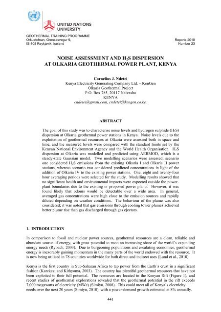
NOISE ASSESSMENT AND H 2 S DISPERSION 

AT OLKARIA GEOTHERMAL POWER PLANT, KENYA 

Cornelius J. Ndetei 

Kenya Electricity Generating Company Ltd. – KenGen 

Olkaria Geothermal Project 

P.O. Box 785, 20117 Naivasha 

KENYA 

cndetei@gmail.com, cndetei@kengen.co.ke, 

ABSTRACT 

The goal of this study was to characterise noise levels and hydrogen sulphide (H 2 S) 

dispersion at Olkaria geothermal power stations in Kenya. Noise levels due to the 

exploitation of geothermal resources at Olkaria were assessed both in space and 

time, and the measured levels were compared with the standard limits set by the 

Kenyan National Environment Agency and the World Health Organisation. H 2 S 

dispersion at Olkaria was modelled and predicted using AERMOD, which is a 

steady-state Gaussian model. Two modelling scenarios were assessed, scenario 

one considered H 2 S emissions from the existing Olkaria I and Olkaria II power 

stations, whereas scenario two considered predicted concentrations in light of the 

addition of Olkaria IV to the existing power stations. One, eight and twenty-four 

hour averaging periods were selected for the study. Modelling results showed that 

no significant health and environmental impacts were expected outside the powerplant 

boundaries due to the existing or proposed power plants. However, it was 

found likely that odours would be detectable over a wide area. In general, 

averaged gas concentrations were high close to the emission sources and rapidly 

diluted depending on weather conditions. The behaviour of the plume was also 

considered; it was noted that gas emissions through cooling tower plumes achieved 

better plume rise than gas discharged through gas ejectors. 

1. INTRODUCTION 

In comparison to fossil and nuclear power sources, geothermal resources are a clean, reliable and 

abundant source of energy, with great potential to meet an increasing share of the world´s expanding 

energy needs (Rybach, 2003). Due to burgeoning populations and escalating economies, geothermal 

energy is inexorably gaining momentum in the many parts of the world endowed with the resource. It 

is now being utilised in 78 countries worldwide for both direct and indirect uses (Lund et al., 2010). 

Kenya is the first country in Sub-Saharan Africa to tap power from the Earth’s crust in a significant 

fashion (Karekezi and Kithyoma, 2003). The country has plentiful geothermal resources that have not 

been exploited to their full potential. The resources are located in the Kenyan Rift (Figure 1), and 

recent studies of geothermal explorations revealed that the geothermal potential in the rift exceeds 

7,000 megawatts of electricity (MWe) (Simiyu, 2008). This could meet all of Kenya’s electricity 

needs over the next 20 years (Simiyu, 2010), with a power-demand growth estimated at 8% annually. 

441

Ndetei 442 Report 23 

The Least Cost Power Development Plan (2010- 

2030) prepared by the Government of Kenya, 

indicates that geothermal plants have the lowest 

unit cost and, therefore, are suitable for base 

load and, as such, are recommended for 

additional expansion (Republic of Kenya, 2010). 

Geothermal energy in Kenya is primarily 

utilised for electricity production, currently 202 

MWe. Direct uses of geothermal energy in the 

country include greenhouses, drying agricultural 

products, swimming, therapeutic bathing, and 

aquaculture. About 14 geothermal sites have 

been identified in the Kenyan Rift (Figure 1). 

These prospect fields from south to north are 

Lake Magadi, Suswa, Longonot, Olkaria, 

Eburru, Badlands, Menengai, Arus Bogoria, 

Lake Baringo, Korosi, Paka, Silali, 

Emuruangogolak, Namarunu and Barrier 

Volcano. Only the Olkaria geothermal field has 

been developed. The other fields are at various 

reconnaissance and surface exploration stages, 

except for Eburru where exploration drilling has 

been undertaken. 

The main environmental concerns arising from 

geothermal operations are associated with noise 

and the discharge of non-condensable gases 

such as hydrogen sulphide (H 2 S), carbon dioxide FIGURE 1: Kenya geothermal fields and prospects 

(CO 2 ) and methane (CH 4 ) into the atmosphere. 

(Lagat, 2004) 

Geothermal fluids also contain small proportions of ammonia, mercury, radon and boron (Komurcu 

and Akpinar, 2009). CO 2 , which is usually the major constituent of the gas present in geothermal 

fluids, and CH 4 , a minor constituent, both require attention because of their roles as greenhouse gases 

(Giroud and Arnórsson, 2005). Among all non-condensable gases emitted due to geothermal 

exploitation, H 2 S has the greatest environmental concern not only because of its noxious smell in low 

concentrations but also due to its toxicity and health impacts at high concentrations, and its tendency 

to concentrate in hollows and low-lying areas due to its high density (Kristmannsdóttir et al., 2000). 

Some projects have been objected to by nearby populations due to the discharge of H 2 S in high 

concentrations, such as in Puna in Hawaii (Anderson, 1991), or were prevented, as at Milos in Greece 

(Marouli and Kaldellis, 2001). As a way of determining environmental impacts associated with noise 

and hydrogen sulphide, various modelling techniques have been employed in distinct parts of the 

world such as in Mexico (Gallegos-Ortega et al., 2000) and Iceland (Nyagah, 2006) among others. 

This study focuses on assessing noise and H 2 S dispersion at the existing Olkaria I and Olkaria II 

power plants and the proposed Olkaria IV power plant in Kenya. 

2. AIMS AND OBJECTIVES 

The goal of this study is to assess noise levels and hydrogen sulphide concentrations at Olkaria 

geothermal field in Kenya, and to model hydrogen sulphide (H 2 S) dispersion in the area. In order to 

accomplish this aim, the following specific objectives will be achieved: 

• Assessment of the temporal and spatial distributions of near ground noise and H 2 S due to 

exploitation of Olkaria I and Olkaria II power stations;

Report 23 443 Ndetei 

• Prediction of H 2 S concentrations due to emissions from the existing Olkaria I and Olkaria II 

power stations and the proposed Olkaria IV power station, using a Gaussian dispersion model; 

and 

• Assessment of any potential health and environmental impacts due to H 2 S emissions from the 

power plants. 

3. BACKGROUND 

3.1 Environmental impacts and health implications of hydrogen sulphide 

Hydrogen sulphide (H 2 S) is produced naturally and as a result of human activity (WHO, 2003). 

Geothermal development is associated with emissions of hydrogen sulphide; the most important points 

of emission in plants are chimneys for venting non-condensable gases, cooling towers, silencers and 

traps in the vapour duct (Nyagah, 2006). Noise sources include the cooling towers and the plant 

housing the turbines. H 2 S, as discussed in detail by WHO (2003), is a colourless, flammable gas, with 

a characteristic odour of rotten eggs at low concentrations, and it is toxic in high concentrations. It is 

rapidly oxidised in air and in solution and is corrosive to many metals; it may discolour paint by its 

reaction with the metals present in the pigments. Because of its high density and negative buoyancy, 

H 2 S can accumulate in low-lying areas such as cellars and basements, and can be imperceptible at 

lethal concentrations (Hunt, 2001). The measurement units for H 2 S in the air are parts per million 

(ppm) or milligrams per cubic metre (mg/m 3 ). At an air temperature of 20°C and 101.3 kPa, 1 ppm of 

H 2 S is equivalent to 1.4 mg/m 3 , hence 1mg/m 3 of the gas is equivalent to 0.71 ppm (WHO, 2003). 

This conversion was adopted in this report. The concentration of the gas in air in unpolluted areas is 

very low, between 0.03 and 0.1 μg/m 3 . 

According to WHO (1981), the toxic effects of H 2 S vary according to the dosage and are classified in 

scientific literature into three categories, namely acute, sub-acute and chronic (for further details, see 

WHO (1981)). Chambers and Johnson (2009) reported that exposure to lower concentrations of 

hydrogen sulphide could result in eye irritation, sore throat, coughing, nausea, shortness of breath, and 

fluid in the lungs. However, long-term, low-level exposure could result in fatigue, loss of appetite, 

headaches, irritability, poor memory, and dizziness (Chambers and Johnson, 2009). 

In humans, H 2 S is unlikely to bio-concentrate because it is excreted through the urine, intestines and 

expired air (WHO, 2003). However, it can be a nuisance at very low concentrations of about 0.3 ppm. 

Table 1 summarises the human health effects of H 2 S at various concentrations. 

There are no ambient air quality standards for H 2 S currently in force in Kenya. Hence, WHO 

guidelines and standards have been adopted in many studies in Kenya. According to WHO (2000) 

guidelines, 24-hour average concentrations should not be permitted to exceed 0.1 ppm beyond the 

immediate power station boundary. The National Institute for Occupational Safety and Health 

(NIOSH), and the American Conference of Governmental and Industrial Hygienists (ACGIH) air 

quality standards for the protection of occupational health give limits of 10 ppm for H 2 S in 

atmospheric air (Webster, 1995). Thus, in workplaces, H 2 S concentrations should not exceed 10 ppm 

over an 8 hour period for staff working five days a week. 

3.2 Noise impacts on health and the associated environmental regulations in Kenya 

Noise is associated with both auditory and non-auditory impacts. Exposure to noise levels of 

relatively high degrees can lead to direct hearing loss or hearing impairment (Ismail et al., 2009). The 

non-auditory impacts include annoyance and disruption of basic activities such as sleep, rest, 

communication, concentration, and might affect health and physiological well-being (WHO, 1999;


TABLE 1: Health impacts of H 2 S at several key concentrations (Chambers and Johnson, 2009) 

H 2 S concent. 

(ppm) 

0.0047 

10 – 20 

50 – 100 

150 – 250 

320 – 530 

500 

530 – 1000 

800 

>1000 

Effects on humans 

Recognition threshold concentration at which 50% of most humans can detect the 

characteristic odour of hydrogen sulphide, normally described as resembling that of 

a rotten egg 

Threshold for eye irritation 

Eye damage 

Olfactory nerve is paralysed after a few inhalations; sense of smell disappears, often 

together with awareness of danger 

Leads to pulmonary oedema with the possibility of death 

30 to 60 minute exposure can result in headache, dizziness, and staggering followed 

by unconsciousness and respiratory failure 

Causes strong stimulation of the central nervous system and rapid breathing leading 

to lack of breath 

Lethal concentration for 50% of humans after 5 minutes exposure 

Causes immediate collapse with loss of breathing (even following inhalation of a 

single breath of H 2 S gas) 

Muzet, 2007). Acute noise exposure has been shown to induce physiological responses such as 

increased blood pressure and heart rate (Haralabidis et al., 2008). Since acute exposure to noise has 

been linked to transient increases in blood pressure and levels of stress hormones in experimental 

settings, it has been hypothesized that long-term exposure to noise may have adverse effects on health 

(Babisch, 2000). Key environmental regulations concerned with regulating noise levels include the 

first and second Schedule of Environment Management and Co-ordination (noise and excessive 

vibration pollution) Regulations of 2009, as set up by the Kenyan National Environmental 

Management Authority (NEMA) (Republic of Kenya, 2009). According to the first schedule, noise 

levels should not exceed 35 dB(A) during the night (20:01 to 06:00 hours) in residential or commercial 

zones. Similarly, daytime levels (06:01 to 20:00 hours) should not exceed 45 dB(A) in indoor 

residential zones, 50 dB(A) in outdoor residential zones or 60 dB(A) in commercial zones. However, 

the second schedule requires that the maximum permissible noise levels for construction sites during 

night time (18:01 to 06:00 hours) should not exceed 35 dB(A) in residential zones or 65 dB(A) in 

commercial zones (Republic of Kenya, 2009). Noise levels during the day (06:01 to 18:00 hours) for 

construction sites should not exceed 60 dB(A) in residential zones or 75 dB(A) in 

commercial/industrial zones. Note that noise is measured in decibels (dB), and the measurements are 

averaged over a certain time period, hence the units are in dB(A). The World Bank finances most 

geothermal projects in developing countries, including Kenya. Consequently, such projects should 

comply with the World Bank and WHO guidelines. Table 2 summarises World Bank and WHO noise 

exposure limit standards at the workplace and in residential areas. 

TABLE 2: World Bank and WHO noise exposure standards (World Bank, 1998; World Bank, 2007) 

Receptor 

Residential, 

institutional and 

educational 

Industrial and 

commercial 

Maximum allowable L * eq (hourly) in dB(A) 

World Bank 

World Health Organization 

Day time 

(07:00-22:00 hrs) 

Night time 

(22:00-07:00 hrs) 

Day time 

(07:00-22:00 hrs) 

Night time 

(22:00-07:00 hrs) 

55 45 50 45 

* L eq is the equivalent continuous sound pressure level 

70 70 85 85


3.3 Situation in Kenya 

In Kenya, geothermal development has been successfully carried out in the Olkaria field. The field is 

located in the Naivasha district, which is among the densely populated districts of the country 

supporting 376,243 people, according to the 2009 population census (KNBS, 2009), and is 27 km 

south of Naivasha town. The Olkaria field, also referred as the Greater Olkaria geothermal area 

(GOGA), covers an area of 

approximately 80 km 2 (Simiyu, 

2008). The Olkaria field has been 

demarcated into seven sub-fields, 

namely Olkaria East, Olkaria West, 

Olkaria Northwest, Olkaria 

Northeast, Olkaria Central, Olkaria 

Domes and Olkaria Southwest 

(Opondo, 2007), shown in Figure 2. 

For ease of discussion, the Olkaria 

field has been broadly categorised 

into four sub-areas, namely Olkaria 

I, Olkaria II, Olkaria III and 

Olkaria IV. The resource from 

Olkaria field is being utilised 

mainly for electric power 

generation (202 MWe), but also for 

direct use (18 MWt) (Simiyu, 

2010). The proven geothermal 

FIGURE 2: Location of the geothermal fields in the 

Greater Olkaria geothermal area (Opondo, 2007) 

resource in the geothermal field is more than 450 MWe (Simiyu, 2010) and accelerated development 

is envisaged in the near future. 

Olkaria I power plant is located in the East field and has three units, each generating 15 MWe, 

whereas Olkaria II power plant is located in the Northeast field and has three units, each generating 35 

MWe. The three units in Olkaria I were commissioned in 1981, 1983 and 1985, respectively, while 

two of the units in Olkaria II were commissioned in 2003 (Simiyu, 2010), and the third unit was 

commissioned in May 2010. Both Olkaria I and II power plants are owned and operated by the Kenya 

Electricity Generating Company (KenGen), which is partly owned by the state (70%) and partly by the 

private sector (30%). The company is in the process of developing two 70 MWe units at Olkaria IV 

(Olkaria Domes) that are expected to be commissioned in 2012/2013 (Simiyu, 2010). Olkaria III 

power plant generates 48 MWe and is located in the West field; it is operated by Ormat, an 

independent power producer. Oserian Development Company, which specialises in flower farming 

for export purposes, generates 4 MWe for its internal uses. 

Olkaria geothermal field is a sensitive area, and studies have been carried out to establish the effects of 

noise and air pollution arising from geothermal exploitation. Kollikho and Kubo (2001) conducted a 

study to investigate the effects of geothermal emissions from cooling towers and gas ejectors on 

flowers cultivated within the vicinity of Olkaria. Their results did not show any significant difference 

in the yield of flowers grown 600 and 1200 m away from the emission sources. 

3.4 Proximity to residential areas 

The existing Olkaria I and Olkaria II power plants are located inside Hell’s Gate National Park, which 

is a protected area for wildlife conservation (Figure 3). Olkaria II power plant is located about 5 km 

south of Lake Naivasha, the only fresh water lake in the Kenyan Rift Valley. About 3 km northwest 

of the power station is the Oserian Development Company, which is a commercially vital floricultural


farm that grows high quality cut 

flowers for export to Europe. There 

are some residential areas and 

community settlements neighbouring 

Olkaria geothermal field, shown in 

Figure 3. The approximate distance 

between Olkaria I and Olkaria II 

power stations is 3.3 km, while the 

distance between Olkaria II and the 

site for Olkaria IV is about 7 km. 

It is important to determine whether 

noise and H 2 S emissions pose any 

significant impact for humans, flora 

or fauna. Air dispersion models have 

been used routinely in environmental 

impact assessments, ecological risk 

analysis and emergency planning. 

The models are also useful in 

properly designing and configuring 

sources of pollution to minimise 

ambient impacts (ADEQ, 2004) and 

effectively predict the impacts of 

hydrogen sulphide on both the 

workers inside the plants and the 

nearby population (Ermak et al., 1980; 

Gallegos-Ortega et al., 2000). Air 

dispersion modelling is used by many 

regulatory agencies as a means of 

assessing the impact of a facility on the 

air quality of the surrounding area, and to 

determine the compliance status. Such 

models are a reliable basis for developing 

and making decisions about 

environmental management and 

sustainability and to provide information 

on real-time emission abatement 

strategies. 

FIGURE 3: Olkaria power stations and the neighbouring 

communities (For co-ordinates of emission 

sources, see Table 3) 

4. STUDY AREA 

4.1 Location and geological setting 

of Olkaria 

This study focuses on the Olkaria 

geothermal area in Kenya located on the 

floor of the rift valley, about 120 km 

northwest of Nairobi. Of particular 

interest is the existing Olkaria I and 

Olkaria II power stations and the 

FIGURE 4: Olkaria and its vicinity (Were, 2007) 

proposed Olkaria IV power station. Figure 4 shows the location of Olkaria and the surrounding 

region, while Figure 5 shows the volcano-tectonic map of Olkaria.


Geothermal resources at Olkaria are 

associated with the Olkaria rhyolitic volcanic 

complex, which consists of a series of lava 

flows and domes, the youngest of which has 

been dated at about 250±100 years ago 

(Simiyu, 2008). Clarke et al. (1990) described 

the geology of Olkaria as being characterised 

by numerous eruptive volcanic centres of 

Quaternary age. The geothermal field is 

located within a remnant of a caldera complex 

intersected by N-S rifting faults. These faults 

are conduits for numerous eruptions that have 

formed pumice and ryholite domes within the 

Olkaria volcanic complex. The area has a 

thick cover of pyroclastic ash that is thought 

to have erupted from volcanic centres outside 

Olkaria, namely Suswa and Longonot. The 

Olkaria volcanic complex is considered to be 

bounded by arcuate faults forming a ring or a 

caldera structure. Within this structure, a 

magmatic heat source might be represented by 

intrusions at depth. Faults and fractures are 

prominent in the area with general N-S and E- 

W trends, but there are also some inferred 

faults striking NW-SE. Other structures in the 

Olkaria area include the Ol’Njorowa gorge 

that trends NW-SE and may represent 

a fault, the Ololbutot fault that trends 

N-S, the ENE-WSW trending Olkaria 

fault, the WNW-ESE trending gorge 

farm fault, and Olkaria fractures. 

FIGURE 5: Volcano-tectonic map of Olkaria field 

(modified from Clarke et al., 1990) 

4.2 Noise and H 2 S monitoring 

Near ground noise levels and H 2 S 

concentrations are monitored in and 

around Olkaria I and II power stations 

using manually operated samplers. 

There are about 18 sites in total for 

monitoring H 2 S at Olkaria I and II 

power stations and its neighbourhood. 

The sites at Olkaria I include the MVrig 

workshop, power station, Olkaria I 

administration offices, seal pit 1, seal 

pit 2, well OW-10, well OW-22, 

scientific laboratories and a general 

store. At Olkaria II, identified sites 

FIGURE 6: Location of noise and H 

include a compressor room, hot well 

2 S monitoring sites 

pit unit 1, hot well pit unit 2, cooling 

towers, power house, Olkaria II administration offices and Kenya Wildlife Service (KWS) Olkaria 

gate. Monitoring is also carried out in residential areas such as Lake View and Lake Side housing 

estates. Figure 6 shows the monitoring sites for noise levels and H 2 S concentrations.


The main sources of noise include the power house (the building that houses electricity generators and 

turbines), steam separators and the cooling towers, whereas the main sources of hydrogen sulphide are 

the cooling towers and the power house. Although there might be other sources of noise and H 2 S such 

as from drilling operations and well testing, these are only temporary and typically last for days. Thus, 

the main emphasis is on the assessment of noise from the permanent operations of the power stations 

while H 2 S sources are the cooling towers or the gas ejectors. At Olkaria I the gas ejector and the plant 

are essentially co-located, whereas at Olkaria II, gas ejection occurs in the cooling towers so that the 

actual H 2 S sources in the aggregation are different for the two power stations; however, this does not 

change the way the H 2 S modelling is undertaken. 

5. METHODOLOGY 

5.1 Theoretical approach to air dispersion 

Air pollutant plume dispersion equations have been undertaken by numerous researchers. By 

performing a mass balance on a small control volume, a simplified diffusion equation, which describes 

a continuous cloud of material dispersing in a turbulent flow, can be written as (Macdonald, 2003): 

 

+ = 

 

+ 

+ (1) 

 

where 

= Along-wind coordinate measured in wind direction from the source; 

 

= Cross-wind coordinate direction; 

 

= Vertical coordinate measured from the ground; 

(, , ) = Mean concentration of diffusing substance at a point (x,y,z) (kg/m 3 ); 

, = Diffusivities in the direction of the y- and z- axes (m 2 /s); 

 

= Mean wind velocity along the x-axis (m/s); and 

 

= Source/sink term (kg/m 3 s). 

A term by term interpretation of Equation 1 is: 

 

+ 

 

 

 

, 

 

Time rate of change and advection of the cloud by the mean wind; 

Turbulent diffusion of material relative to the centre of the pollutant cloud; and 

Source term which represents the net production of pollutants. 

In deriving Equation 1, it is assumed that the pollutant concentrations do not affect the flow field 

(passive dispersion), molecular diffusion and longitudinal (along-wind) diffusion are negligible, flow 

is incompressible, wind velocities and concentrations can be decomposed into a mean and fluctuating 

component with the average value of the fluctuating (stochastic) component equal to zero, turbulent 

fluxes are linearly related to the gradients of the mean concentrations and the mean lateral (V) and 

vertical (W) wind velocities are zero. 

An analytical solution to Equation 1 gives the Gaussian plume model. For a continuous point-source 

released at the origin in a uniform (homogenous) turbulent flow, the solution to Equation 1, as given 

by Macdonald (2003), is: 

 

− 

(,,) = 

 

4 

4 (/) − 

4 (/) (2)


where is the source pollutant emission rate. 

The turbulent diffusivities and are unknown in most flows; in the atmospheric boundary 

layer, is not constant, but increases with height above the ground. In addition, and increase 

with distance from the source, because the diffusion is affected by different scales of turbulence in the 

atmosphere as the plume grows. If we define the lateral dispersion coefficient function, , and the 

vertical diffusion coefficient function, , as follows (Seinfeld and Pandis, 2006): 

= 2 

 

= 2 

 

 

(3) 

then the final form of the Gaussian plume equation, for an elevated plume released at = is 

(Seinfeld and Pandis, 2006): 

 

(,,) = − 

2 

2 − ( − ) 

+− ( + ) 

(4) 

2 

2 

In this expression, a second z-exponential term has been added to account for the fact that a pollutant 

cannot diffuse downward through the ground at = 0, but is assumed to be reflected. This “image” 

term can be visualised as an equivalent source located at = − below the ground. 

Equation 4 is the Gaussian plume formula for a continuous point source. The plume height is the 

sum of the actual stack height plus any plume rise Δ due to initial buoyancy and momentum of 

the release. The wind speed is taken to be the mean wind speed at the height of the stack. 

Considering concentrations at ground level (where receptors are) and assuming = 0 , we obtain 

(Macdonald, 2003): 

(, , = 0) = 

 

 

− 

2 

− 

2 

(5) 

A general non-Gaussian model, which allows for vertical variation, is expressed as: 

(, , ) = 

 

− 

() (6) 

√2 

2 

Here () is a normalized function that describes the vertical distribution of material in the plume. 

The rate of transfer of a pollutant through any vertical plane downwind from the source is a constant 

steady state, and this constant should equal the emission rate of the source, Q. Thus: 

= (7) 

, 

where the integration is performed over the y-z plane, perpendicular to the plume axis. 

5.2 Available data and sources 

The AERMOD dispersion model (Cimorelli et al., 2004) was used to simulate H 2 S dispersion and 

concentrations due to emissions from the existing Olkaria I and Olkaria II power plants and the


proposed Olkaria IV power plant. The AERMOD dispersion model requires surface data on 

meteorology (wind speed (m/s), wind direction (degrees), dry bulb temperature (°C), relative humidity 

(%), station pressure (mbar), opaque cloud cover (tenth), cloud ceiling height (m), and global 

horizontal radiation (W/m 2 )), atmospheric stability obtained from upper air soundings, surface 

characteristics (surface roughness, Bowen ratio and albedo) and information about the source being 

modelled, including pollutant emission rate, location and exit velocity. Surface meteorological data 

was obtained from the Environment unit of KenGen, Olkaria. The data was produced by an automatic 

weather station located at X-2, about 500 m northwest of the Olkaria II power plant, for the period 

November 2003 to September 2006. For modelling purposes, surface meteorology data for the period 

1 st to 30 th November 2003 was used since it was complete. Upper air data was available from 

Dagoretti meteorological weather station, located at latitude 1.30°S and 36.75°E, which is more than 

120 km from the area of interest. Since the upper air sounding station was located far from the area of 

interest, upper air data was estimated by the model using the available surface meteorological data. A 

Bowen ratio of 4, albedo of 0.28 and surface roughness of 0.3 were used in the modelling. Table 3 

gives a description of the emission parameters that were used to model dispersion. 

In Olkaria, the non-condensable gases such as H 2 S, CO 2 , CH 4 and N 2 present in geothermal fluid 

(Sinclair Knight and Partners, 1994) are disposed of by discharging them into cooling tower fans for 

dispersal into the atmosphere. There is a difference between Olkaria I and Olkaria II power stations 

due to the ways in which they dispose of waste hydrogen sulphide. Olkaria II power station 

discharges the non-condensable H 2 S with evaporative emissions in the cooling tower plume, whereas 

Olkaria I power station discharges the H 2 S through gas ejectors located in the main power station 

building. The cooling tower plumes have a substantial plume-rise compared with the plume-rise from 

the gas ejectors (Sinclair Knight and Partners, 1994). However, for modelling purposes, the two 

power plants have been treated in the same way. 

5.3 Model descriptions 

The selection of an air dispersion model depends on many factors such as the nature of the pollutant, 

characteristics of emission sources and the relationship between the emission source and the receptor. 

Other factors influencing model selection include meteorological and topographic complexities of the 

area, complexity of the source distribution, spatial scale and resolution required for the analysis, level 

of detail and accuracy required for the analysis, and averaging times to be modelled. Some of the well 

known models include ISCST3, AERMOD, ASPEN, CALPUFF, UTM-TOX, and CAMx. In this 

study, AERMOD was applied to model H 2 S dispersion. 

AERMOD stands for AERMIC Model, where AERMIC is the American Meteorological Society/EPA 

Regulatory Model Improvement Committee. AERMOD was developed in 1995, reviewed in 1998 

and formally proposed by the United States Environmental Protection Agency (US EPA) as a 

replacement for the Industrial Source Complex Short Term model (ISC-ST3) in 2000 (Bluett et al., 

2004). 

A detailed description of AERMOD was given by Cimorelli et al. (2004). AERMOD is a steady-state 

plume model. In the stable boundary layer (SBL), it assumes the concentration distribution to be 

Gaussian both vertically and horizontally. In the convective boundary layer (CBL), the horizontal 

distribution is also assumed to be Gaussian, but the vertical distribution is described with a bi- 

Gaussian probability density function (pdf). Additionally, in the CBL, AERMOD monitors “plume 

lofting”, whereby a portion of plume mass, released from a buoyant source, rises to and remains near 

the top of the boundary layer before becoming mixed into the CBL. AERMOD also tracks any plume 

mass that penetrates into the elevated stable layer, and then allows it to re-enter the boundary layer 

when and if appropriate. For sources in both the CBL and the SBL, AERMOD treats the enhancement


TABLE 3: Emission parameters used to model dispersion from existing Olkaria I and Olkaria II 

power stations and the proposed Olkaria IV power station (Holmes Air Sciences, 2009) 

Parameter 

S 

of lateral dispersion resulting from plume meander. AERMOD handles the computation of pollutant 

impacts in both flat and complex terrain within the same modelling framework. Using a relatively 

simple approach, AERMOD incorporates current concepts about flow and dispersion in complex 

terrains. Where appropriate, the plume is modelled as either impacting and/or following the terrain. 

The model also has the ability to characterise the Planetary Boundary Layer (PBL) through both 

surface and mixed layer scaling (Cimorelli et al., 2004). 

5.3.1 AERMET 

Olkaria I 

Olkaria II 

(Units 1 and 2) 

Olkaria II 

(Unit 3) 

Proposed 

Olkaria IV 

(Units 1 and 2) 

Height of emission 

point above grade (m) 

19 16 19 19 

Height of grade above 

sea level (m) 

1932 2005 2005 2035 

Exit velocity (m/s) 20 9.2 8.6 8.6 

Exit temperature (K) 375 304 303 303 

Diameter of discharge 

point at tip (m) 

0.2 9.14 9.64 9.64 

Mass emission rate of 

H 2 S for each of the 3 

emission points for 

Olkaria I, 12 emission 

points for Olkaria II, 

and 8 emission points 

for Olkaria IV, 

respectively (g/s) 

4.46 3.55 3.55 7.1 

Coordinates of 

discharge points 

(in UTM, zone 37 

south of the equator) 

Easting 

200420 

200412 

200404 

Northing 

9901480 

9901500 

9901525 

Easting 

199365 

199370 

199376 

199382 

199387 

199393 

199399 

199404 

Northing 

9904727 

9904717 

9904708 

9904699 

9904689 

9904680 

9904670 

9904661 

Easting 

199356 

199349 

199342 

199336 

Northing 

9904744 

9904755 

9904766 

9904777 

Easting 

203538 

203533 

203527 

203521 

203516 

203510 

203504 

203499 

Northing 

9898811 

9898820 

9898830 

9898839 

9898849 

9898858 

9898867 

9898877 

AERMET is the meteorological pre-processor of AERMOD. The input data to AERMET, as 

described by Cimorelli et al. (2004), consists of surface roughness, albedo and Bowen ratio, plus 

standard meteorological observations including wind speed, wind direction, temperature and cloud 

cover. AERMET then calculates the PBL parameters which include friction velocity ( ∗ ), Monin- 

Obukhov length (), convective velocity scale ( ∗ ), temperature scale ( ∗ ), mixing height ( ), and 

surface heat flux (). These scaling parameters are used to construct vertical profiles of wind speed 

(), lateral and vertical turbulent fluctuations ( , ) , potential temperature gradient (/), and 

potential temperature (). Detailed mathematical expressions of these PBL parameters are described 

by Cimorelli et al. (2004).


5.3.2 AERMAP 

AERMAP is the terrain pre-processor of AERMOD and uses gridded terrain data to calculate a 

representative terrain-influence height (hc) for each receptor with which AERMOD computes receptor 

specific Hc values. AERMOD handles the computation of pollutant impacts in both flat and complex 

terrain within the same modelling framework (Cimorelli et al. (2004)) as illustrated in Figure 7. In 

complex terrain, AERMOD incorporates the concept of the dividing streamline for stability-stratified 

conditions. Where appropriate, the plume is modelled as a combination of two limiting cases: a 

horizontal plume (terrain impacting) and a terrain-following (terrain responding) plume. In stable 

flow, a two-layer structure develops in which the lower layer remains horizontal while the upper layer 

tends to rise over the terrain. In neutral and unstable conditions Hc = 0. AERMOD captures the effect 

of flow above and below the dividing streamline by weighting the plume concentration associated with 

two possible extreme states of the boundary layer: horizontal plume and terrain-following. The 

relative weighting of a horizontal plume and terrain-following depends on the degree of atmospheric 

stability, the wind speed and the plume height relative to the terrain. The weighting of the two plume 

states depends on the amount of mass residing in each state. This mass partitioning is based on the 

relationship between the critical dividing streamline height (Hc) and the vertical concentration 

distribution at a receptor. 

FIGURE 7: AERMOD horizontal plume state 

and terrain-following state approaches 

(Cimorelli et al., 2004) 

FIGURE 8: Treatment of terrain in AERMOD; 

construction of the weighting factor used in 

calculating total concentration 

(Cimorelli et al., 2004) 

During convective conditions the concentration at an elevated receptor is the average of the 

contributions from the two states. As plumes above Hc encounter terrain and are deflected vertically, 

there is also a tendency for plume material to approach the terrain surface and to spread out around the 

sides of the terrain. To simulate this, concentration estimates always contain a component from the 

horizontal state and, hence, under no condition is the plume allowed to completely approach the 

terrain-following state. For flat terrain, the contributions from the two states are equal in value and are 

equally weighted. Figure 8 illustrates how the weighting factor is constructed and its relationship to 

the estimate of concentrations as a weighted sum of two limiting plume states. 

The modelling used the default regulatory dispersion option for H 2 S concentration output and assumed 

a flat terrain height. The Universal Transverse Mercator (UTM) projection for zone 37 south of the 

equator was employed using the world geodetic system of 1984 (WGS-84). The prediction of H 2 S 

concentrations was simulated using 1-hour average, 8-hour average and 24-hour average time periods. 

A uniform Cartesian grid spacing of 200 m by 200 m was considered over a length of 16 km by 16 km 

extending from E192000 m to E208000 m and N9896000 m to N9912000 m.


6. RESULTS 

6.1 Temporal variation of meteorology, noise and hydrogen sulphide concentrations at Olkaria 

Figure 9 shows the monthly 

mean air temperature and 

relative humidity from 

meteorological station X-2, 

Olkaria. Measurements were 

made at twice-daily intervals: 

09:00 and 15:00 local standard 

time. The maximum temperature 

recorded in the area ranged 

between 21.6 and 28.5°C, with a 

mean value of 24.8°C. 

Minimum temperature in the 

area ranged between 8.3 and 

14.1°C, with a mean value of 

FIGURE 9: Monthly mean air temperature and relative humidity 

from meteorological station X-2, Olkaria 

11.1°C. Relative humidity at the station ranged between 55.2 and 86.0%, with a mean value of 73%. 

Thus, the temperatures and relative humidity showed relatively modest seasonal variations. 

Figure 10 shows the mean 

monthly variation of noise at 

Olkaria I power station and its 

vicinity. Noise level data was 

collected from March 1995 to 

April 2010. The main source of 

noise at Olkaria I is the power 

station building which houses 

the turbines and generators and, 

as indicated in Figure 10, noise 

levels at the monitoring site near 

the power station occasionally FIGURE 10: Mean monthly variation of noise at 

exceeded the recommended 

Olkaria I and its vicinity 

WHO limit of 85 dB(A). However, moving farther away from the source, noise levels decayed as 

illustrated by measurements mostly below 75 dB(A) recorded at the administration block and at the 

KWS gate monitoring sites. Noise levels in the Lake View residential area were below 50 dB(A), the 

limit set by the Kenyan National Environment Agency. 

Figure 11 shows the mean monthly variation of noise at Olkaria II power station. Noise data at 

Olkaria II power station were collected from September 2003 to April 2010. The noise levels at 

Olkaria II power station were 

within the WHO limit of 85 

dB(A), as illustrated by 

measurements taken at the 

monitoring sites at the power 

station, the cooling tower and 

the Olkaria II administration 

block. Although the overall 

noise level at Olkaria II was 

within permitted limits, Figure 

11 shows a pronounced increase 

in intensity from mid 2006 

onwards. A comparison of FIGURE 11: Mean monthly variation of noise at Olkaria II


Figures 10 and 11 indicates that noise intensity was relatively higher at Olkaria I than at Olkaria II. 

This might be attributed to the newer technology in use at Olkaria II. 

FIGURE 12: Daily variation of H 2 S at Olkaria II 

FIGURE 13: Daily variation of H 2 S at Olkaria I 

H 2 S emissions from Olkaria I 

and Olkaria II power stations 

were monitored from April 1997 

and September 2003 to April 

2010, respectively. Figures 12 

and 13 show the daily variations 

of H 2 S concentrations at Olkaria 

II and Olkaria I power stations. 

The highest recorded value of 

H 2 S at Olkaria II was 2.2 ppm 

while at Olkaria I, the highest 

recorded value was 4.4 ppm. 

Thus, H 2 S concentrations at 

Olkaria I and Olkaria II power 

stations were below the National 

Institute of Occupational Safety 

and Health (NIOSH) standards 

of 10 ppm averaged over a 24- 

hour period for employees 

working eight hours per day for 

five days in a week. Similarly, 

H 2 S concentrations outside the 

plant boundaries were far below 

the WHO (2000) limit of 0.1 

ppm. H 2 S concentrations at 

Olkaria II were relatively low, 

occasionally below the detection 

threshold. However, this was not the case with Olkaria I power station where H 2 S emission was 

evident (Figure 13) and the detection threshold of 0.0047 ppm (Chambers and Johnson, 2009) was 

frequently exceeded. 

6.2 Spatial variation of noise and hydrogen sulphide at Olkaria 

The spatial variations of the noise levels and H 2 S concentrations emanating from Olkaria I and Olkaria 

II power stations are shown in Figures 14 to 17. The spatial variation of noise at Olkaria I and Olkaria 

II power stations indicates that noise was emitted mainly from the cooling towers and the power 

house, spreading to the surrounding areas in a decaying logarithmic pattern. Noise levels near Olkaria 

II power station were in the range of 80 dB(A), and decreased with distance so that noise levels at the 

FIGURE 14: Spatial variation of noise (dB(A)) 

at Olkaria II 

FIGURE 15: Spatial variation of noise (dB(A)) 

at Olkaria I


KWS gate, about 600 m away, were in the range of 42 dB(A), as indicated in Figure 14. Figure 15 

shows the spatial variation of noise at Olkaria I power station and its surroundings. 

The annual average concentration of hydrogen sulphide near Olkaria II power plant was in the range 

of 0.03 ppm, and dispersed such that the concentration at the KWS gate, about 600 m from Olkaria II 

power station, was 0.002 ppm (Figure 16). Relatively high concentrations of hydrogen sulphide were 

recorded at Olkaria I, as indicated in Figure 17, with the highest concentration of 0.36 ppm recorded at 

close proximity to the power station. 

FIGURE 16: Spatial variation of H 2 S (ppm) 

at Olkaria II 

FIGURE 17: Spatial variation of H 2 S (ppm) 

at Olkaria I 

6.3 Wind distribution at Olkaria 

Figure 18 shows the 

seasonal windroses for 

the Olkaria area for 

the periods (a) 

December to February 

(b) March to May (c) 

June to July and (d) 

September to November. 

These periods 

represent the four 

main seasons in 

Kenya. Automatic 

wind speed and wind 

direction data collected 

from November 

2003 to September 

2005 were used to plot 

the windroses. Figure 

18 indicates that the 

general wind pattern at 

Olkaria is southeast in 

all seasons except 

summer (December- 

January - February) 

when the wind pattern 

randomised, characterised 

by southeasterly and northwesterly directions. 

FIGURE 18: Seasonal windroses for X-2 weather station, Olkaria; 

(a) December to February (b) March to May (c) June to July 

(d) September to November


6.4 Modelling results from AERMOD 

6.4.1 Air dispersion results from the existing Olkaria I (Units 1, 2, 3 ) and Olkaria II 

(Units 1, 2, 3) power stations 

Air dispersion results for Olkaria 

I (Units 1, 2 and 3) and Olkaria 

II (Units 1, 2 and 3) generally 

predicted that high 

concentrations of H 2 S would 

occur near the power plants; the 

concentration values for Olkaria 

I measured higher than those for 

Olkaria II. 

Figure 19 shows that the highest 

predicted H 2 S concentrations, 

averaged over a one-hour period, 

equalled 1356 μg/m 3 (0.963 

ppm), due to emissions from the 

three units of Olkaria I and the 

three units of Olkaria II. This 

highest concentration occurred 

at E199400 m and N99046000 

m, which is close to the Olkaria I 

power station. The plume 

concentrated about 500 m from 

the power plant and spread 

mainly eastwards as it decayed 

so that at a distance of 500 m, 

the concentration was 242 μg/m 3 

(0.172 ppm). 

H 2 S concentrations averaged 

over 8-hour periods indicated 

that the highest concentration 

equalled 297 μg/m 3 (0.211 ppm), 

sourced at E199400 m and 

N9904800 m, which is near 

Olkaria I power station (Figure 

20). The plume emitted from 

Olkaria I power station 

dispersed to the northeast; the 

values were relatively small so 

that at a distance of about 600 m 

from the station, the 

concentrations were 60 μg/m 3 

(0.043 ppm). At Olkaria II 

power station, H 2 S 

concentrations were lower than 

at Olkaria I, and concentrated 

near the station. The highest 8- 

hour average concentration 

FIGURE 19: Predicted 1-hour averaged H 2 S concentrations 

(μg/m 3 ) due to emissions from the existing Olkaria I 

(Units 1, 2, 3) and Olkaria II (Units 1, 2, 3) power stations 



(Units 1, 2, 3) and Olkaria II (Units 1, 2, 3) power stations


value at Olkaria II equalled 219 

μg/m 3 (0.155 ppm) and dispersed 

uniformly so that at a distance of 

about 500 m, the concentration was 

47 μg/m 3 (0.033 ppm). 

For the case of 24-hour averaged 

concentrations, the highest 

predicted H 2 S concentration 

equalled 118 μg/m 3 (0.0838 ppm), 

located at E200200 m and 

N9901600 m which is close to 

Olkaria I power station (Figure 21). 

The plume from Olkaria I power 

station spread northeast; at a 

distance of 400 m northeast of the 

station, the concentration was in the 

range of 50 μg/m 3 (0.035 ppm). At 

Olkaria II power station, the highest 

H 2 S concentration was 99 μg/m 3 , 

decaying to a concentration of 50 

μg/m 3 at 300 m from the station. 

The dispersion model indicated that 

24-hour average H 2 S concentrations 



(Units 1, 2, 3) and Olkaria II (Units 1, 2, 3) power stations 

due to emissions from Olkaria I and Olkaria II power stations were far below the WHO threshold limit 

value of 150 μg/m 3 (0.1 ppm) beyond the power station boundary (WHO, 2000). 

6.4.2 Air dispersion results from the existing Olkaria I (Units 1, 2, 3), Olkaria II (Units 1, 2, 3) 

and the proposed Olkaria IV (Units 1, 2) power stations 

H 2 S dispersion results for the two 

existing power plants, Olkaria I 

(units 1, 2, 3) and Olkaria II (units 

1, 2, 3), and for the proposed 2 

units of Olkaria IV indicated 1- 

hour averaged concentrations of 

1948 μg/m 3 (1.383 ppm) at 

E203400 m and N9898800 m; this 

was in close proximity to the 

proposed Olkaria IV power station 

(Figure 22). At a distance of 500 

m from the Olkaria IV power plant, 

the 1-hour average predicted a 

concentration of 340 μg/m 3 (0.241 

ppm). The dispersion model 

indicated that the residential area 

about 4 km southwest of Olkaria I 

had minimal or no health impacts 

due to emissions from the three 

power plants. 



(Units 1, 2, 3), Olkaria II (Units 1, 2, 3) and the proposed 

Olkaria IV (Units 1 and 2) power stations


Figure 23 shows 8-hour averaged 

H 2 S concentration levels due to 

emissions from the existing two 

power plants (Olkaria I and Olkaria 

II) and the proposed power plant 

(Olkaria IV). The plume dispersion 

model indicated that the highest 8– 

hour averaged hydrogen sulphide 

concentration of 644 μg/m 3 (0.457 

ppm) would be in close proximity 

to Olkaria IV (E203400 m, 

N9898800 m). A zone of H 2 S was 

also noted northeast of Olkaria I 

power station, attaining a maximum 

ground level concentration of 130 

μg/m 3 (0.092 ppm) at about 2 km 

from the station. 

Figure 24 shows the predicted 24- 

hour averaged concentration of H 2 S 

due to emissions from Olkaria I 

(units 1, 2, 3), Olkaria II (units 1, 2, 

3) and Olkaria IV (units 1, 2) power 

plants. The dispersion model 

estimated the highest concentration 

as 410 μg/m 3 (0.291 ppm). A 

plume of H 2 S spread northeast of 

Olkaria I and north of Olkaria II. 

The model predicted that the 

residential area extending from 500 

m south and southwest of Olkaria I 

would be free of atmospheric 

pollution from the three power 

plants, while settlements inside the 

power plant boundary of the 

proposed Olkaria IV were within 

the boundary for 150 μg/m 3 H 2 S 

concentration. 


(μg/m 3 ) due to emissions from the existing Olkaria I (Units 1, 

2, 3), Olkaria II (Units 1, 2, 3) and the proposed Olkaria IV 

(Units 1 and 2) power stations 

The addition of Olkaria IV power 

plant to the existing Olkaria I and 

Olkaria II power plants will neither 

impact Akira ranch nor the Oserian 

farm or Lake View estate. As 

shown in Figure 24, the proposed 

site for Olkaria IV power station is 

located on private land, outside the 

Kenya Wildlife Service (KWS) 


(μg/m 3 ) due to emissions from the existing Olkaria I (Units 

1, 2, 3), Olkaria II (Units 1, 2, 3) and the proposed 

Olkaria IV (Units 1 and 2) power stations 

boundary. According to WHO 

guidelines (WHO, 2000), 24-hour 

averaged H 2 S concentrations should not exceed 150 μg/m 3 (0.1 ppm) beyond the immediate power 

station boundary. If the WHO assessment criterion is to be met, then it implies a relocation plan 

should exist for some human settlements residing within the power plant boundaries of the proposed 

Olkaria IV power station.


7. IMPLICATIONS 

The highest predicted H 2 S concentration for 1-hour averaged values from the existing Olkaria I and II 

power plants was 1356 μg/m 3 (0.963 ppm). According to the dispersion simulation, the addition of 

Olkaria IV power station to the existing power stations would increase the highest 1-hour 

concentration to 1948 μg/m 3 (1.383 ppm). It was predicted that this worst condition would be 

concentrated within the plant boundary and would decrease rapidly with distance from the power 

plant. Thus, H 2 S concentrations due to exploitation of Olkaria IV power station would have negligible 

impacts on the surrounding communities located outside the plant boundary. Predicted H 2 S 

concentrations, using 8-hour and 24-hour averages due to exploitation of Olkaria I, Olkaria II and 

Olkaria IV power stations, did not exceed 150 μg/m 3 (0.1 ppm) beyond the plant boundaries. Hence, 

the more stringent WHO (2000) threshold limit of 0.1 ppm for a 24-hour period would not be 

exceeded outside the plant boundary. The predicted concentrations due to exploitation of the three 

power plants were also far below the less stringent standards set by the National Institute for 

Occupational Safety and Health (NIOSH); by their criterion, air quality standards should not exceed 

10 ppm (14,000 μg/m 3 ) over an eight hour period for employees working 40 hours per week (Webster, 

1995). 

Generally, the highest predicted H 2 S concentrations at Olkaria were close to the main gas emissions, 

and decreased rapidly with distance. A similar dispersion pattern has been reported both in Kenya 

(Marani et al., 2000) and in Sousaki, Greece (Alessandro et al., 2009). The concentrations were 

predicted to be too low to affect vegetation outside the plant boundaries; that is, concentrations outside 

the plant boundaries were less than 0.03 ppm (42.0 μg/m 3 ) averaged over a 24-hour period. This is 

supported by earlier studies carried out in the study area to assess health impacts to vegetation due to 

H 2 S emissions arising from Olkaria I and Olkaria II power stations (Kubo and Kollikho, 2001). 

Similarly, there is no danger to human life or the environment since 0.1 ppm is not exceeded outside 

the plant boundary using 24-hour averaging. Although no health impacts were predicted to occur, as 

stated earlier, the model predicted that odour which is a nuisance would be presently detectable over a 

wide area (Figures 21 and 24) as indicated by predicted H 2 S concentrations above the detection 

threshold of 0.0047 ppm (6.58 μg/m 3 ). 

Plume spread was more distributed at Olkaria I than at Olkaria II power station and, similarly, H 2 S 

concentrations were more pronounced at the former than at the latter. Thus, it can be concluded that 

disposing of H 2 S emissions through cooling tower plumes, as is done at Olkaria II, is an improved 

discharging method, and will achieve much greater plume rise than when discharging the gas through 

gas ejectors as is the case at Olkaria I. 

8. CONCLUSIONS AND RECOMMENDATIONS 

Noise assessment and H 2 S dispersion measurements were carried out in Olkaria. The spatial and 

temporal variation of noise indicated that the levels fell within the WHO limits near the power station 

boundary. In rare cases where the limit was exceeded, especially at the Olkaria I power station, the 

use of personal protective equipment such as ear muffs is recommended. Noise levels in residential 

areas did not exceed the limits set by the Kenyan National Environment Agency. 

Predictions of H 2 S concentrations were undertaken by considering two cases: (1) predicting 

concentrations due to emissions from the existing Olkaria I and Olkaria II power stations and (2) 

predicting concentrations due to emissions from the existing Olkaria I and Olkaria II power stations 

and the proposed Olkaria IV power station. These two cases were simulated for 1-hour, 8-hour and 

24-hour averages. In all cases of 1-hour, 8-hour and 24-hour averaging scenarios, the predicted 

hydrogen sulphide concentrations were less than 10 ppm (14,000 μg/m 3 ), the threshold for workers 

according to the National Institute for Occupational Safety and Health (NIOSH). In general, the


averaged concentrations were high near the emission sources and were diluted depending on weather 

conditions, especially temperature, wind speed and direction. Generally, the predicted concentrations 

due to emissions from Olkaria I and Olkaria II power plants were below 0.1 ppm (150 μg/m 3 ) outside 

the power plant boundary. The AERMOD model captured the main features of H 2 S dispersion at 

Olkaria, and used them to predict H 2 S concentrations due to the existing Olkaria I and Olkaria II 

power plants and the proposed Olkaria IV power plant. The model predicted relatively high H 2 S 

concentrations within the plant boundary, decreasing rapidly farther away from the power station such 

that concentrations at 500 m away would cause no significant impacts to humans, flora or fauna. 

Similar conclusions due to the exploitations of Olkaria I and Olkaria II power stations were reached by 

Marani et al. (2000) who studied H 2 S concentrations around the Olkaria field and found no significant 

impacts to the environment. 

The AERMOD dispersion model is a useful tool that may be employed in environmental and social 

impact assessments for new geothermal developments and for environmental audits of existing power 

plants, and can be used in decision-making based on sound theoretical grounds. The accuracy of the 

predicted modelling results is based on the quality of the input data used, especially meteorological 

data. Hence, well-equipped automatic weather stations and a high-quality database should be in 

operation for effective dispersion modelling. 

ACKNOWLEDGEMENTS 

I am greatly indebted to the United Nations University Geothermal Training Programme (UNU-GTP) 

and the Government of Iceland for awarding me the fellowship to undertake the six months specialised 

training in geothermal research. I wish to thank my employer, Kenya Electricity Generating Company 

Ltd. (KenGen) for granting me sabbatical leave to attend the training. Special thanks go to the UNU- 

GTP Director, Ingvar B. Fridleifsson, and the Deputy-Director, Lúdvík S. Georgsson. I cannot forget 

crucial contributions made by other UNU-GTP staff including Thórhildur Ísberg, Dorthe H. Holm, 

Markús A.G. Wilde and Ingimar G. Haraldsson. My sincere appreciation goes to my supervisor, Dr. 

Matthew J. Roberts, for his wise ideas, guidance and support. Earnest appreciation goes to the UNU- 

GTP class of 2010 for their memorable co-operation. Finally, I express my deepest gratitude to my 

workmates, friends, relatives and my family. To my dear wife and daughter, thanks for your 

encouragement, sacrifice, and unconditional love during my six months of study. Above all, I glorify 

the Mighty God for His love, care and mercy that has seen me to this point. 

REFERENCES 

ADEQ (Arizona Department of Environmental Quality), 2004: Air dispersion modeling guidelines for 

Arizona air quality permits. Air assessment section, air quality division, Arizona Department of 

Environmental Quality, December 2004, Arizona, 63 pp. 

Alessandro, L., Brusca, L., Kyriakopoulos, K., Michas, G., and Papadakis, G., 2009: Hydrogen 

sulphide as natural air contaminant in volcanic/geothermal areas: the case of Sousaki, Corinthia- 

Greece. Environ. Geol., 57, 1723-1728. 

Anderson, I., 1991: Blowout blights future of Hawaii’s geothermal power. New Sci., 17, 1778, 17. 

Babisch, W., 2000: Traffic noise and cardiovascular disease: Epidemiological review and synthesis. 

Noise Health, 2, 9-32. 

Bluett, J., Gimson, N., Fisher, G., Heydenrycn, C., Freeman, T., and Godfrey, J., 2004: Good practice 

guide for atmospheric dispersion modelling. Ministry of Environment, Manatū Mō Te Taiao, 

Wellington, New Zealand, webpage: www.mfe.govt.nz, 152 pp.


Chambers, T., and Johnson, J.A., 2009: Environmental mitigation monitoring: Hydrogen sulphide 

(H 2 S) gas dispersion potentials and release scenarios of Pacific OCS region’s oil & gas platforms and 

pipelines located in the Santa Barbara channel and Santa Maria basin, California. MMS OCS, report 

2009-021, 62 pp. 

Cimorelli, A.J., Perry, S.G., Venkatram, A., Weil, J.C., Paine, R.J., Wilson, R.B., Lee, R.F., Peters, 

W.D., Brode, R.W., and Paumier, J.O., 2004: AERMOD: Description of model formulation. U.S. 

Environmental Protection Agency, report-454/R-03-004, 91 pp. 

Clarke, M.C.G., Woodhall, D.G., Allen, D., and Darling, G., 1990: Geological, volcanological and 

hydrogeological controls of the occurrence of geothermal activity in the area surrounding Lake 

Naivasha, Kenya. Ministry of Energy, Nairobi, 138 pp. 

Ermak, D.L, Nyholm, R.A., and Gudilsen, P.H., 1980: Potential air quality impacts of large-scale 

geothermal energy development in the Imperial Valley, California, USA. Atmos. Environ., 14, 1321- 

1330. 

Gallegos-Ortega, R., Quintero-Nuñez, M., and García-Cueto, O., 2000: H 2 S dispersion model at Cerro 

Prieto geothermoelectric power plant. Proceedings of the World Geothermal Congress 2000, Kyushu- 

Tohoku, Japan, 579-584. 

Giroud, N., and Arnórsson, S., 2005: Estimation of long-term CO 2 and H 2 S release during operation 

of geothermal power plants. Proceedings of the World Geothermal Congress 2005, Antalya, Turkey, 

6 pp. 

Haralabidis, A.S., Dimakopoulou, K., Vigna-Taglianti, F., Giampaolo, M., Borgini, A., and Dudley, 

M.L., 2008: Acute effects of night-time noise exposure on blood pressure in populations living near 

airports. European Heart Journal, 29, 658-664. 

Holmes Air Sciences, 2009: Olkaria II geothermal power plant project hydrogen sulphide dispersion 

study of the effects of emissions from unit 3. Air quality impact assessment report. Mitsubishi Heavy 

Industries, Ltd., Japan, Holmes Air Sciences, Australia, 41 pp. 

Hunt, T.M., 2001: Five lectures on environmental effects of geothermal utilization. UNU-GTP, 

Iceland, report 1-2000, 109 pp. 

Ismail, A.R., Nor, M.J.M., Mansor, M.R.A., Tahir, M.F.M., and Zulkifli, R., 2009: Environmental 

noise assessment and modelling in Malaysia: A comparative monitoring study. European J. Scientific 

Research 30-2, 236-244. 

Karekezi, S., and Kithyoma, W., 2003: Renewable energy development. Workshop for African 

Energy Experts on Operationalizing the NEPAD Energy Initiative, Dakar, Senegal, 27 pp. 

KNBS, 2009: Population and housing census for 2009. Kenya National Bureau of Statistics, website: 

www.knbs.or.ke. 

Kollikho P., and Kubo, B., 2001: Olkaria geothermal power plant gaseous emissions – A flower trial 

case study. Geoth. Res. Council, Transactions, 25, 257-261. 

Komurcu, M.I., and Akpinar, A., 2009: Importance of geothermal energy and its environmental 

effects in Turkey. Renewable Energy, 34, 1611-1615. 

Kristmannsdóttir, H., Sigurgeirsson, M., Ármannsson, H., Hjartarsson, H., and Ólafsson, M., 2000: 

Sulphur gas emissions from geothermal power plants in Iceland. Geothermics, 29, 525-538. 

Lagat, J.K., 2004: Geology, hydrothermal alteration and fluid inclusion studies of Olkaria Domes 

geothermal field, Kenya. University of Iceland, Msc Thesis, UNU-GTP, Iceland, report 1, 71 pp. 

Lund, J.W., Freeston, D.H., and Boyd, T.L., 2010: Direct utilization of geothermal energy 2010 

worldwide review. Proceedings of the World Geothermal Congress 2010, Bali, Indonesia, 23 pp. 

Macdonald, R., 2003: Theory and objectives of air dispersion modelling. The University of Western 

Ontario, Faculty of Engineering, 27 pp., website: 

www.engga.uwo.ca/people/esavory/MME474A_Part1.pdf.


Marani, M., Tole, M., and Ogalo, L., 2000: Concentrations of hydrogen sulphide in air around the 

Olkaria geothermal field, Kenya. Proceedings of the World Geothermal Congress 2000, Kyushu- 

Tohoku, Japan, 649-661. 

Marouli, C., and Kaldellis, J.K., 2001: Risk in the Greek electricity production sector. Proceedings of 

the 7 th International Conference on Environmental Science and Technology, Ermoupolis, Syros Island, 

Greece, 305–314. 

Muzet, A., 2007: Environmental noise, sleep and health. Sleep Medicine Reviews, 11, 135-142. 

Nyagah, E.M., 2006: Hydrogen sulphide dispersion and modelling for Nesjavellir power station using 

Gaussian and numerical models. Report 15 in: Geothermal Training in Iceland 2006. UNU-GTP, 

Iceland, 291-314. 

Opondo, K.M., 2007: Corrosive species and scaling in wells at Olkaria, Kenya and Reykjanes, 

Svartsengi and Nesjavellir, Iceland. University of Iceland, MSc thesis, UNU-GTP, Iceland, report 2, 

76 pp. 

Republic of Kenya, 2009: Environment management and co-ordination (noise and excessive vibration 

pollution control) regulations, 2009. Government of Kenya, Legal notice no. 61, Government printer, 

Nairobi, 23 pp. 

Republic of Kenya, 2010: Least cost power development plan, study period 2010-2030. Ministry of 

Energy, Kenya, 147 pp. 

Rybach, L., 2003: Geothermal energy: sustainability and the environment. Geothermics, 32, 463- 

470. 

Seinfeld, J.H., and Pandis, S.N., 2006: Atmospheric diffusion. In: Atmospheric chemistry and 

physics, from air pollution to climate change (2 nd ed.), John Wiley and Sons, Inc. 828-899. 

Simiyu, S.M., 2008: Kenya’s geothermal expansion strategy for developing 1260 MWe by 2018. 

Geoth. Res. Council, Transactions, 32, 369-372. 

Simiyu, S.M., 2010: Status of geothermal exploration in Kenya and future plans for its development. 

Proceedings of the World Geothermal Congress 2010, Bali, Indonesia, 11 pp. 

Sinclair Knight and Partners, 1994: Environmental assessment for north east Olkaria power 

development project. Report for the KenGen Company Ltd., RSP International Ltd., 800 pp. 

Webster, J.G., 1995: Chemical impacts of geothermal development. In: Brown, K.L. (convenor), 

Environmental aspects of geothermal development. World Geothermal Congress 1995, IGA precongress 

course, Pisa, Italy, 79-95. 

Were, J.O., 2007: The speciation of trace elements in spent geothermal fluids and implications for 

environmental health around Olkaria, Kenya. University of Iceland, MSc Thesis, UNU-GTP, Iceland, 

report 1, 73 pp. 

WHO, 1981: Hydrogen sulphide. World Health Organization, Geneva, Environmental health criteria, 

no. 19. 

WHO, 1999: Guidelines for community noise. World Health Organization, Geneva, 141 pp. 

WHO, 2000: Air quality guidelines for Europe (2 nd ed.). WHO regional publications, European 

Series no. 91, 273 pp. 

WHO, 2003: Hydrogen sulphide: human health aspects. World Health Organization, Geneva, 

Concise international chemical assessment document 53, 35 pp., website: 

www.who.int/ipcs/publications/cicad/en/cicad53.pdf. 

World Bank, 1998: Pollution prevention and abatement handbook. Toward cleaner production, 

World Bank Group, Washington, DC, 471 pp. 

World Bank, 2007: Environmental, health and safety (EHS) guidelines, World Bank Group, 

Washington, DC, 99 pp.

noise assessment and h2s dispersion at olkaria ... - Orkustofnun

Create successful ePaper yourself

Delete template?

Save as template?