Amber Tools Guide - NCI National Facility

AmberTools Users’ Manual
Version 1.0, April 1, 2008
AmberTools consists of several independently developed packages that work well with Amber
itself. The suite can also be used to carry out complete molecular mechanics investigations
(using NAB), but which are restricted to gas-phase or generalized Born solvent models.
The main components of AmberTools are listed below. Our plan is that future versions will
contain more functionality, and will be better integrated with one another. If you are interested
in contributing to this effort, please contact Dave Case.
NAB (Nucleic Acid Builder)
Thomas J. Macke, 1 W.A. Svrcek-Seiler, 2 Russell A. Brown, 3 István Kolossváry, 4 Yannick J.
Bomble 5 and David A. Case 5
LEaP and gleap
Wei Zhang, 6 Tingjun Hou, 7 Christian Schafmeister, 8 Wilson S. Ross, and David A. Case
Antechamber
Junmei Wang 10
Ptraj
Thomas E. Cheatham, III 11
1 Kosmix Corporation, Mountain View, CA 94041; 2 University of Vienna, A-1010 Vienna,
Austria ; 3 Sun Microsystems, Inc., Menlo Park, CA 94025 ; 4 Budapest University of
Technology and Economics, Budapest, Hungary. Present address: D.E. Shaw Research, LLC,
New York, NY; 5 The Scripps Research Institute, La Jolla, CA 92037; 6 Univ. of Texas, Health
Center at Houston; 7 Univ. of California, San Diego; 8 University of Pittsburgh; 10 Univ. of
Texas, Southwestern Medical Center; 11 University of Utah
3

Notes
• Most of the programs included here can be redistributed and/or modified under the terms
of the GNU General Public License; a few components have other open-source licenses.
See the LICENSE_at file for details. The programs are distributed in the hope that they
will be useful, but WITHOUT ANY WARRANTY; without even the implied warranty of
MERCHANTABILITY or FITNESS FOR A PARTICULAR PURPOSE.
• Some of the force field routines were adapted from similar routines in the MOIL program
package: R. Elber, A. Roitberg, C. Simmerling, R. Goldstein, H. Li, G. Verkhivker, C.
Keasar, J. Zhang and A. Ulitsky, "MOIL: A program for simulations of macromolecules"
Comp. Phys. Commun. 91, 159-189 (1995).
• The "trifix" routine for random pairwise metrization is based on an algorithm designed
by Jay Ponder and was adapted from code in the Tinker package; see M.E. Hodsdon, J.W.
Ponder, and D.P. Cistola, J. Mol. Biol. 264, 585-602 (1996) and http://dasher.wustl.edu/tinker/.
• The "molsurf" routines for computing molecular surface areas were adapted from routines
written by Paul Beroza. The "sasad" routine for computing derivatives of solvent accessible
surface areas was kindly provided by S. Sridharan, A. Nicholls and K.A. Sharp. See
J. Computat. Chem. 8, 1038-1044 (1995).
• The preprocessor (ucpp) was written by Thomas Pornin ,
http://www.di.ens.fr/∼pornin/ucpp/, and is distributed under a separate, BSD-style license.
See ucpp-0.7/README for details.
• The cifparse routines to deal with mmCIF formatted files were written by John Westbrook,
and are distributed with permission. See cifparse/README for details.
• Sun, Sun Microsystems and Sun Performance Library are trademarks or registered trademarks
of Sun Microsystems, Inc. in the United States and other countries.
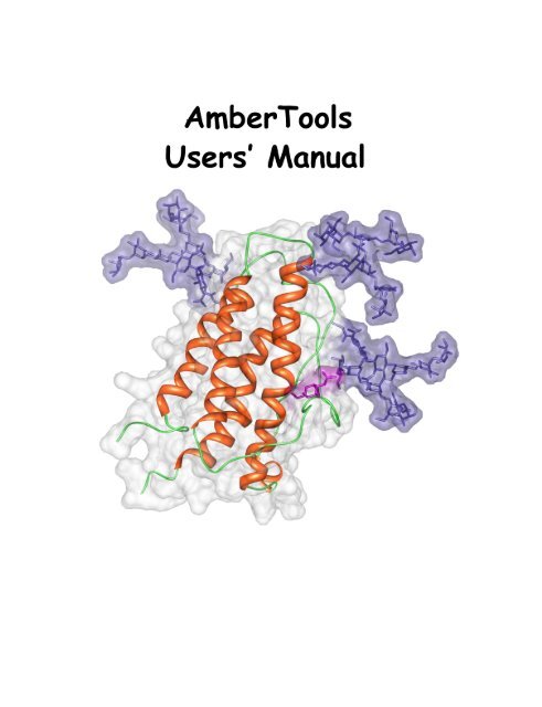
Cover Illustration
Erythropoietin exists as a mixture of glycosylated variants (glycoforms), [1] and glycosylation
is known to modulate its biological function. [2, 3] The three high-mannose N-linked
oligosaccharides (Man_9 GlcNAc_2 ) are shown in purple, the single O-linked glycan (alpha-
GalNAc) is shown in pink. The structure in the image represents a single glycoform that is
the origin from which all others are generated. The protein structure was solved by NMR
(pdbid: 1BUY) [4] and the glycans were added to the protein using the GLYCAM Web-tool
(http://www.glycam.com) with energy minimization performed using the AMBER FF99 parameters
[5] for the protein and the GLYCAM06 parameters [6] for the oligosaccharides. Figure
made by the Woods group using Chimera. [7]
4

Contents
Contents 5
1 Getting started 11
1.1 Information flow in Amber . . . . . . . . . . . . . . . . . . . . . . . . . . . . 11
1.1.1 Preparatory programs . . . . . . . . . . . . . . . . . . . . . . . . . . . 12
1.1.2 Simulation programs . . . . . . . . . . . . . . . . . . . . . . . . . . . 12
1.1.3 Analysis programs . . . . . . . . . . . . . . . . . . . . . . . . . . . . 13
1.2 Installation . . . . . . . . . . . . . . . . . . . . . . . . . . . . . . . . . . . . 13
1.3 Contacting the developers . . . . . . . . . . . . . . . . . . . . . . . . . . . . . 14
2 Specifying a force field 15
2.1 Specifying which force field you want in LEaP . . . . . . . . . . . . . . . . . 16
2.2 The AMOEBA potentials . . . . . . . . . . . . . . . . . . . . . . . . . . . . . 17
2.3 The Duan et al. (2003) force field . . . . . . . . . . . . . . . . . . . . . . . . 17
2.4 The Yang et al. (2003) united-atom force field . . . . . . . . . . . . . . . . . . 18
2.5 1999 force fields and recent updates . . . . . . . . . . . . . . . . . . . . . . . 18
2.6 The 2002 polarizable force fields . . . . . . . . . . . . . . . . . . . . . . . . . 20
2.7 Force related to semiempirical QM . . . . . . . . . . . . . . . . . . . . . . . . 21
2.8 GLYCAM-06 and GLYCAM-04EP force fields for carbohydrates . . . . . . . 21
2.9 Ions . . . . . . . . . . . . . . . . . . . . . . . . . . . . . . . . . . . . . . . . 24
2.10 Solvent models . . . . . . . . . . . . . . . . . . . . . . . . . . . . . . . . . . 27
2.11 Obsolete force field files . . . . . . . . . . . . . . . . . . . . . . . . . . . . . 29
2.11.1 The Cornell et al. (1994) force field . . . . . . . . . . . . . . . . . . . 29
2.11.2 The Weiner et al. (1984,1986) force fields . . . . . . . . . . . . . . . . 30
3 LEaP 31
3.1 Introduction . . . . . . . . . . . . . . . . . . . . . . . . . . . . . . . . . . . . 31
3.2 Concepts . . . . . . . . . . . . . . . . . . . . . . . . . . . . . . . . . . . . . 31
3.2.1 Commands . . . . . . . . . . . . . . . . . . . . . . . . . . . . . . . . 31
3.2.2 Variables . . . . . . . . . . . . . . . . . . . . . . . . . . . . . . . . . 32
3.2.3 Objects . . . . . . . . . . . . . . . . . . . . . . . . . . . . . . . . . . 32
3.3 Basic instructions for using LEaP . . . . . . . . . . . . . . . . . . . . . . . . . 36
3.3.1 Building a Molecule For Molecular Mechanics . . . . . . . . . . . . . 37
3.3.2 Amino Acid Residues . . . . . . . . . . . . . . . . . . . . . . . . . . 37
3.3.3 Nucleic Acid Residues . . . . . . . . . . . . . . . . . . . . . . . . . . 38
3.4 Commands . . . . . . . . . . . . . . . . . . . . . . . . . . . . . . . . . . . . 38
3.4.1 add . . . . . . . . . . . . . . . . . . . . . . . . . . . . . . . . . . . . 38
5

CONTENTS
3.4.2 addAtomTypes . . . . . . . . . . . . . . . . . . . . . . . . . . . . . . 39
3.4.3 addIons . . . . . . . . . . . . . . . . . . . . . . . . . . . . . . . . . . 40
3.4.4 addIons2 . . . . . . . . . . . . . . . . . . . . . . . . . . . . . . . . . 40
3.4.5 addPath . . . . . . . . . . . . . . . . . . . . . . . . . . . . . . . . . . 40
3.4.6 addPdbAtomMap . . . . . . . . . . . . . . . . . . . . . . . . . . . . . 40
3.4.7 addPdbResMap . . . . . . . . . . . . . . . . . . . . . . . . . . . . . . 41
3.4.8 alias . . . . . . . . . . . . . . . . . . . . . . . . . . . . . . . . . . . . 42
3.4.9 bond . . . . . . . . . . . . . . . . . . . . . . . . . . . . . . . . . . . 42
3.4.10 bondByDistance . . . . . . . . . . . . . . . . . . . . . . . . . . . . . 42
3.4.11 check . . . . . . . . . . . . . . . . . . . . . . . . . . . . . . . . . . . 42
3.4.12 combine . . . . . . . . . . . . . . . . . . . . . . . . . . . . . . . . . . 43
3.4.13 copy . . . . . . . . . . . . . . . . . . . . . . . . . . . . . . . . . . . . 43
3.4.14 createAtom . . . . . . . . . . . . . . . . . . . . . . . . . . . . . . . . 44
3.4.15 createResidue . . . . . . . . . . . . . . . . . . . . . . . . . . . . . . . 44
3.4.16 createUnit . . . . . . . . . . . . . . . . . . . . . . . . . . . . . . . . . 44
3.4.17 deleteBond . . . . . . . . . . . . . . . . . . . . . . . . . . . . . . . . 44
3.4.18 desc . . . . . . . . . . . . . . . . . . . . . . . . . . . . . . . . . . . . 44
3.4.19 groupSelectedAtoms . . . . . . . . . . . . . . . . . . . . . . . . . . . 45
3.4.20 help . . . . . . . . . . . . . . . . . . . . . . . . . . . . . . . . . . . . 46
3.4.21 impose . . . . . . . . . . . . . . . . . . . . . . . . . . . . . . . . . . 46
3.4.22 list . . . . . . . . . . . . . . . . . . . . . . . . . . . . . . . . . . . . . 47
3.4.23 loadAmberParams . . . . . . . . . . . . . . . . . . . . . . . . . . . . 47
3.4.24 loadAmberPrep . . . . . . . . . . . . . . . . . . . . . . . . . . . . . . 47
3.4.25 loadOff . . . . . . . . . . . . . . . . . . . . . . . . . . . . . . . . . . 47
3.4.26 loadMol2 . . . . . . . . . . . . . . . . . . . . . . . . . . . . . . . . . 48
3.4.27 loadPdb . . . . . . . . . . . . . . . . . . . . . . . . . . . . . . . . . . 48
3.4.28 loadPdbUsingSeq . . . . . . . . . . . . . . . . . . . . . . . . . . . . . 48
3.4.29 logFile . . . . . . . . . . . . . . . . . . . . . . . . . . . . . . . . . . 48
3.4.30 measureGeom . . . . . . . . . . . . . . . . . . . . . . . . . . . . . . 49
3.4.31 quit . . . . . . . . . . . . . . . . . . . . . . . . . . . . . . . . . . . . 49
3.4.32 remove . . . . . . . . . . . . . . . . . . . . . . . . . . . . . . . . . . 49
3.4.33 saveAmberParm . . . . . . . . . . . . . . . . . . . . . . . . . . . . . 50
3.4.34 saveOff . . . . . . . . . . . . . . . . . . . . . . . . . . . . . . . . . . 50
3.4.35 savePdb . . . . . . . . . . . . . . . . . . . . . . . . . . . . . . . . . . 50
3.4.36 sequence . . . . . . . . . . . . . . . . . . . . . . . . . . . . . . . . . 50
3.4.37 set . . . . . . . . . . . . . . . . . . . . . . . . . . . . . . . . . . . . . 51
3.4.38 solvateBox and solvateOct . . . . . . . . . . . . . . . . . . . . . . . . 52
3.4.39 solvateCap . . . . . . . . . . . . . . . . . . . . . . . . . . . . . . . . 53
3.4.40 solvateShell . . . . . . . . . . . . . . . . . . . . . . . . . . . . . . . . 53
3.4.41 source . . . . . . . . . . . . . . . . . . . . . . . . . . . . . . . . . . . 54
3.4.42 transform . . . . . . . . . . . . . . . . . . . . . . . . . . . . . . . . . 54
3.4.43 translate . . . . . . . . . . . . . . . . . . . . . . . . . . . . . . . . . . 54
3.4.44 verbosity . . . . . . . . . . . . . . . . . . . . . . . . . . . . . . . . . 55
3.4.45 zMatrix . . . . . . . . . . . . . . . . . . . . . . . . . . . . . . . . . . 55
3.5 Building oligosaccharides and lipids . . . . . . . . . . . . . . . . . . . . . . . 56
6

CONTENTS
3.5.1 Procedures for building oligosaccharides using the GLYCAM 06 parameters
. . . . . . . . . . . . . . . . . . . . . . . . . . . . . . . . . . 57
3.5.2 Procedures for building a lipid using GLYCAM 06 parameters . . . . . 59
3.5.3 Procedures for building a glycoprotein in LEaP. . . . . . . . . . . . . . 60
3.6 Differences between tleap and sleap . . . . . . . . . . . . . . . . . . . . . . . 62
3.6.1 Limitations . . . . . . . . . . . . . . . . . . . . . . . . . . . . . . . . 63
3.6.2 Unsupported Commands . . . . . . . . . . . . . . . . . . . . . . . . . 63
3.6.3 New Commands or New Features of old Commands . . . . . . . . . . 63
3.6.4 New keywords . . . . . . . . . . . . . . . . . . . . . . . . . . . . . . 64
3.6.5 The basic idea behind the new commands . . . . . . . . . . . . . . . . 65
4 Antechamber 67
4.1 Principal programs . . . . . . . . . . . . . . . . . . . . . . . . . . . . . . . . 68
4.1.1 antechamber . . . . . . . . . . . . . . . . . . . . . . . . . . . . . . . 68
4.1.2 parmchk . . . . . . . . . . . . . . . . . . . . . . . . . . . . . . . . . . 70
4.2 A simple example for antechamber . . . . . . . . . . . . . . . . . . . . . . . . 71
4.3 Programs called by antechamber . . . . . . . . . . . . . . . . . . . . . . . . . 74
4.3.1 atomtype . . . . . . . . . . . . . . . . . . . . . . . . . . . . . . . . . 74
4.3.2 am1bcc . . . . . . . . . . . . . . . . . . . . . . . . . . . . . . . . . . 75
4.3.3 bondtype . . . . . . . . . . . . . . . . . . . . . . . . . . . . . . . . . 75
4.3.4 prepgen . . . . . . . . . . . . . . . . . . . . . . . . . . . . . . . . . . 76
4.3.5 espgen . . . . . . . . . . . . . . . . . . . . . . . . . . . . . . . . . . 77
4.3.6 respgen . . . . . . . . . . . . . . . . . . . . . . . . . . . . . . . . . . 77
4.4 Miscellaneous programs . . . . . . . . . . . . . . . . . . . . . . . . . . . . . 78
4.4.1 acdoctor . . . . . . . . . . . . . . . . . . . . . . . . . . . . . . . . . . 79
4.4.2 crdgrow . . . . . . . . . . . . . . . . . . . . . . . . . . . . . . . . . . 80
4.4.3 database . . . . . . . . . . . . . . . . . . . . . . . . . . . . . . . . . . 80
4.4.4 parmcal . . . . . . . . . . . . . . . . . . . . . . . . . . . . . . . . . . 80
4.4.5 residuegen . . . . . . . . . . . . . . . . . . . . . . . . . . . . . . . . 81
4.4.6 translate . . . . . . . . . . . . . . . . . . . . . . . . . . . . . . . . . . 81
5 ptraj 83
5.1 ptraj command prerequisites . . . . . . . . . . . . . . . . . . . . . . . . . . . 85
5.2 ptraj input/output commands . . . . . . . . . . . . . . . . . . . . . . . . . . . 86
5.3 ptraj commands that modify the state . . . . . . . . . . . . . . . . . . . . . . . 88
5.4 ptraj action commands . . . . . . . . . . . . . . . . . . . . . . . . . . . . . . 89
5.5 Correlation and fluctuation facility . . . . . . . . . . . . . . . . . . . . . . . . 98
5.6 Examples . . . . . . . . . . . . . . . . . . . . . . . . . . . . . . . . . . . . . 102
5.6.1 Calculating and analyzing matrices and modes . . . . . . . . . . . . . 102
5.6.2 Projecting snapshots onto modes . . . . . . . . . . . . . . . . . . . . . 102
5.6.3 Calculating time correlation functions . . . . . . . . . . . . . . . . . . 102
5.7 Hydrogen bonding facility . . . . . . . . . . . . . . . . . . . . . . . . . . . . 103
5.8 rdparm . . . . . . . . . . . . . . . . . . . . . . . . . . . . . . . . . . . . . . . 105
7

CONTENTS
6 NAB: Introduction 109
6.1 Background . . . . . . . . . . . . . . . . . . . . . . . . . . . . . . . . . . . . 110
6.1.1 Conformation build-up procedures . . . . . . . . . . . . . . . . . . . . 111
6.1.2 Base-first strategies . . . . . . . . . . . . . . . . . . . . . . . . . . . . 111
6.2 Methods for structure creation . . . . . . . . . . . . . . . . . . . . . . . . . . 112
6.2.1 Rigid-body transformations . . . . . . . . . . . . . . . . . . . . . . . 112
6.2.2 Distance geometry . . . . . . . . . . . . . . . . . . . . . . . . . . . . 113
6.2.3 Molecular mechanics . . . . . . . . . . . . . . . . . . . . . . . . . . . 114
6.3 Compiling nab Programs . . . . . . . . . . . . . . . . . . . . . . . . . . . . . 115
6.4 Parallel Execution . . . . . . . . . . . . . . . . . . . . . . . . . . . . . . . . . 115
6.5 First Examples . . . . . . . . . . . . . . . . . . . . . . . . . . . . . . . . . . 118
6.5.1 B-form DNA duplex . . . . . . . . . . . . . . . . . . . . . . . . . . . 118
6.5.2 Superimpose two molecules . . . . . . . . . . . . . . . . . . . . . . . 119
6.5.3 Place residues in a standard orientation . . . . . . . . . . . . . . . . . 120
6.6 Molecules, Residues and Atoms . . . . . . . . . . . . . . . . . . . . . . . . . 121
6.7 Creating Molecules . . . . . . . . . . . . . . . . . . . . . . . . . . . . . . . . 122
6.8 Residues and Residue Libraries . . . . . . . . . . . . . . . . . . . . . . . . . . 123
6.9 Atom Names and Atom Expressions . . . . . . . . . . . . . . . . . . . . . . . 125
6.10 Looping over atoms in molecules . . . . . . . . . . . . . . . . . . . . . . . . . 126
6.11 Points, Transformations and Frames . . . . . . . . . . . . . . . . . . . . . . . 128
6.11.1 Points and Vectors . . . . . . . . . . . . . . . . . . . . . . . . . . . . 128
6.11.2 Matrices and Transformations . . . . . . . . . . . . . . . . . . . . . . 128
6.11.3 Frames . . . . . . . . . . . . . . . . . . . . . . . . . . . . . . . . . . 129
6.12 Creating Watson Crick duplexes . . . . . . . . . . . . . . . . . . . . . . . . . 130
6.12.1 bdna() and fd_helix() . . . . . . . . . . . . . . . . . . . . . . . . . . . 130
6.12.2 wc_complement() . . . . . . . . . . . . . . . . . . . . . . . . . . . . 131
6.12.3 wc_helix() Overview . . . . . . . . . . . . . . . . . . . . . . . . . . . 132
6.12.4 wc_basepair() . . . . . . . . . . . . . . . . . . . . . . . . . . . . . . . 133
6.12.5 wc_helix() Implementation . . . . . . . . . . . . . . . . . . . . . . . . 136
6.13 Structure Quality and Energetics . . . . . . . . . . . . . . . . . . . . . . . . . 140
6.13.1 Creating a Parallel DNA Triplex . . . . . . . . . . . . . . . . . . . . . 140
6.13.2 Creating Base Triads . . . . . . . . . . . . . . . . . . . . . . . . . . . 141
6.13.3 Finding the lowest energy triad . . . . . . . . . . . . . . . . . . . . . . 143
6.13.4 Assembling the Triads into Dimers . . . . . . . . . . . . . . . . . . . 145
7 NAB: Language Reference 149
7.1 Introduction . . . . . . . . . . . . . . . . . . . . . . . . . . . . . . . . . . . . 149
7.2 Language Elements . . . . . . . . . . . . . . . . . . . . . . . . . . . . . . . . 149
7.2.1 Identifiers . . . . . . . . . . . . . . . . . . . . . . . . . . . . . . . . . 149
7.2.2 Reserved Words . . . . . . . . . . . . . . . . . . . . . . . . . . . . . 149
7.2.3 Literals . . . . . . . . . . . . . . . . . . . . . . . . . . . . . . . . . . 150
7.2.4 Operators . . . . . . . . . . . . . . . . . . . . . . . . . . . . . . . . . 150
7.2.5 Special Characters . . . . . . . . . . . . . . . . . . . . . . . . . . . . 151
7.3 Higher-level constructs . . . . . . . . . . . . . . . . . . . . . . . . . . . . . . 151
7.3.1 Variables . . . . . . . . . . . . . . . . . . . . . . . . . . . . . . . . . 151
8

CONTENTS
7.3.2 Attributes . . . . . . . . . . . . . . . . . . . . . . . . . . . . . . . . . 152
7.3.3 Arrays . . . . . . . . . . . . . . . . . . . . . . . . . . . . . . . . . . . 154
7.3.4 Expressions . . . . . . . . . . . . . . . . . . . . . . . . . . . . . . . . 155
7.3.5 Regular expressions . . . . . . . . . . . . . . . . . . . . . . . . . . . 156
7.3.6 Atom Expressions . . . . . . . . . . . . . . . . . . . . . . . . . . . . 156
7.3.7 Format Expressions . . . . . . . . . . . . . . . . . . . . . . . . . . . . 157
7.4 Statements . . . . . . . . . . . . . . . . . . . . . . . . . . . . . . . . . . . . . 159
7.4.1 Expression Statement . . . . . . . . . . . . . . . . . . . . . . . . . . . 159
7.4.2 Delete Statement . . . . . . . . . . . . . . . . . . . . . . . . . . . . . 160
7.4.3 If Statement . . . . . . . . . . . . . . . . . . . . . . . . . . . . . . . . 160
7.4.4 While Statement . . . . . . . . . . . . . . . . . . . . . . . . . . . . . 160
7.4.5 For Statement . . . . . . . . . . . . . . . . . . . . . . . . . . . . . . . 161
7.4.6 Break Statement . . . . . . . . . . . . . . . . . . . . . . . . . . . . . 162
7.4.7 Continue Statement . . . . . . . . . . . . . . . . . . . . . . . . . . . . 162
7.4.8 Return Statement . . . . . . . . . . . . . . . . . . . . . . . . . . . . . 162
7.4.9 Compound Statement . . . . . . . . . . . . . . . . . . . . . . . . . . . 162
7.5 Structures . . . . . . . . . . . . . . . . . . . . . . . . . . . . . . . . . . . . . 163
7.6 Functions . . . . . . . . . . . . . . . . . . . . . . . . . . . . . . . . . . . . . 164
7.6.1 Function Definitions . . . . . . . . . . . . . . . . . . . . . . . . . . . 164
7.6.2 Function Declarations . . . . . . . . . . . . . . . . . . . . . . . . . . 165
7.7 Points and Vectors . . . . . . . . . . . . . . . . . . . . . . . . . . . . . . . . . 165
7.8 String Functions . . . . . . . . . . . . . . . . . . . . . . . . . . . . . . . . . . 166
7.9 Math Functions . . . . . . . . . . . . . . . . . . . . . . . . . . . . . . . . . . 167
7.10 System Functions . . . . . . . . . . . . . . . . . . . . . . . . . . . . . . . . . 169
7.11 I/O Functions . . . . . . . . . . . . . . . . . . . . . . . . . . . . . . . . . . . 169
7.11.1 Ordinary I/O Functions . . . . . . . . . . . . . . . . . . . . . . . . . . 169
7.11.2 matrix I/O . . . . . . . . . . . . . . . . . . . . . . . . . . . . . . . . . 171
7.12 Molecule Creation Functions . . . . . . . . . . . . . . . . . . . . . . . . . . . 171
7.13 Creating Biopoloymers . . . . . . . . . . . . . . . . . . . . . . . . . . . . . . 172
7.14 Fiber Diffraction Duplexes in NAB . . . . . . . . . . . . . . . . . . . . . . . . 173
7.15 Reduced Representation DNA Modeling Functions . . . . . . . . . . . . . . . 174
7.16 Molecule I/O Functions . . . . . . . . . . . . . . . . . . . . . . . . . . . . . . 175
7.17 Other Molecular Functions . . . . . . . . . . . . . . . . . . . . . . . . . . . . 176
7.18 Debugging Functions . . . . . . . . . . . . . . . . . . . . . . . . . . . . . . . 178
7.19 Time and date routines . . . . . . . . . . . . . . . . . . . . . . . . . . . . . . 179
8 NAB: Rigid-Body Transformations 181
8.1 Transformation Matrix Functions . . . . . . . . . . . . . . . . . . . . . . . . . 181
8.2 Frame Functions . . . . . . . . . . . . . . . . . . . . . . . . . . . . . . . . . 181
8.3 Functions for working with Atomic Coordinates . . . . . . . . . . . . . . . . . 182
8.4 Symmetry Functions . . . . . . . . . . . . . . . . . . . . . . . . . . . . . . . 182
8.4.1 Matrix Creation Functions . . . . . . . . . . . . . . . . . . . . . . . . 183
8.4.2 Matrix I/O Functions . . . . . . . . . . . . . . . . . . . . . . . . . . . 184
8.5 Symmetry server programs . . . . . . . . . . . . . . . . . . . . . . . . . . . . 185
8.5.1 matgen . . . . . . . . . . . . . . . . . . . . . . . . . . . . . . . . . . 185
9

CONTENTS
8.5.2 Symmetry Definition Files . . . . . . . . . . . . . . . . . . . . . . . . 185
8.5.3 matmerge . . . . . . . . . . . . . . . . . . . . . . . . . . . . . . . . . 187
8.5.4 matmul . . . . . . . . . . . . . . . . . . . . . . . . . . . . . . . . . . 188
8.5.5 matextract . . . . . . . . . . . . . . . . . . . . . . . . . . . . . . . . . 188
8.5.6 transform . . . . . . . . . . . . . . . . . . . . . . . . . . . . . . . . . 188
9 NAB: Distance Geometry 189
9.1 Metric Matrix Distance Geometry . . . . . . . . . . . . . . . . . . . . . . . . 189
9.2 Creating and manipulating bounds, embedding structures . . . . . . . . . . . . 190
9.3 Distance geometry templates . . . . . . . . . . . . . . . . . . . . . . . . . . . 195
9.4 Bounds databases . . . . . . . . . . . . . . . . . . . . . . . . . . . . . . . . . 198
10 NAB: Molecular mechanics and dynamics 201
10.1 Basic molecular mechanics routines . . . . . . . . . . . . . . . . . . . . . . . 201
10.2 Typical calling sequences . . . . . . . . . . . . . . . . . . . . . . . . . . . . . 205
10.3 Second derivatives and normal modes . . . . . . . . . . . . . . . . . . . . . . 207
10.4 Low-MODe (LMOD) optimization methods . . . . . . . . . . . . . . . . . . . 209
10.4.1 LMOD conformational searching . . . . . . . . . . . . . . . . . . . . 209
10.4.2 LMOD Procedure . . . . . . . . . . . . . . . . . . . . . . . . . . . . . 210
10.4.3 XMIN . . . . . . . . . . . . . . . . . . . . . . . . . . . . . . . . . . . 211
10.4.4 Sample XMIN program . . . . . . . . . . . . . . . . . . . . . . . . . 211
10.4.5 LMOD . . . . . . . . . . . . . . . . . . . . . . . . . . . . . . . . . . 214
10.4.6 Sample LMOD program . . . . . . . . . . . . . . . . . . . . . . . . . 218
10.4.7 Tricks of the trade of running LMOD searches . . . . . . . . . . . . . 221
11 NAB: Sample programs 223
11.1 Duplex Creation Functions . . . . . . . . . . . . . . . . . . . . . . . . . . . . 223
11.2 nab and Distance Geometry . . . . . . . . . . . . . . . . . . . . . . . . . . . . 224
11.2.1 Refine DNA Backbone Geometry . . . . . . . . . . . . . . . . . . . . 225
11.2.2 RNA Pseudoknots . . . . . . . . . . . . . . . . . . . . . . . . . . . . 228
11.2.3 NMR refinement for a protein . . . . . . . . . . . . . . . . . . . . . . 231
11.3 Building Larger Structures . . . . . . . . . . . . . . . . . . . . . . . . . . . . 235
11.3.1 Closed Circular DNA . . . . . . . . . . . . . . . . . . . . . . . . . . . 235
11.3.2 Nucleosome Model . . . . . . . . . . . . . . . . . . . . . . . . . . . . 239
11.4 Wrapping DNA Around a Path . . . . . . . . . . . . . . . . . . . . . . . . . . 242
11.4.1 Interpolating the Curve . . . . . . . . . . . . . . . . . . . . . . . . . . 242
11.4.2 Driver Code . . . . . . . . . . . . . . . . . . . . . . . . . . . . . . . . 246
11.4.3 Wrap DNA . . . . . . . . . . . . . . . . . . . . . . . . . . . . . . . . 247
11.5 Other examples . . . . . . . . . . . . . . . . . . . . . . . . . . . . . . . . . . 250
Bibliography 251
Index 259
10

1 Getting started
AmberTools is a set of programs for biomolecular simulation and analysis. They are designed
to work well with each other, and with the “regular” Amber suite of programs. You can carry
out a lot of simulation tasks with AmberTools, and can do more extensive simulations with the
combination of AmberTools and Amber itself.
We expect that AmberTools will be dynamic, and change and grow over time. This initial
release consists of programs that have previously been part of Amber (including LEaP,
antechamber and ptraj), along with NAB (Nucleic Acid Builder), which has been released separately.
Each of these packages has been in use for a long time. They are certainly not bug-free,
but you should be able to rely upon them in many circumstances.
The programs here are mostly released under the GNU General Public License (GPL). A
few components are included that are in the public domain or which have other, open-source,
licenses. See the README_at and LICENSE_at files for more information. We hope to add new
functionality to AmberTools as additional programs become available. If you have suggestions
for what might be added, please contact us.
1.1 Information flow in Amber
Understanding where to begin in AmberTools is primarily a problem of managing the flow
of information in this package–see Fig. 1.1. You first need to understand what information is
needed by the simulation programs (sander, pmemd or nab). You need to know where it comes
from, and how it gets into the form that the energy programs require. This section is meant to
orient the new user and is not a substitute for the individual program documentation.
Information that all the simulation programs need:
1. Cartesian coordinates for each atom in the system. These usually come from Xray crystallography,
NMR spectroscopy, or model-building. They should be in Protein Databank
(PDB) or Tripos "mol2" format. The program LEaP provides a platform for carrying out
many of these modeling tasks, but users may wish to consider other programs as well.
2. "Topology": connectivity, atom names, atom types, residue names, and charges. This
information comes from the database, which is found in the amber10/dat/leap/prep directory,
and is described in Chapter 2. It contains topology for the standard amino acids
as well as N- and C-terminal charged amino acids, DNA, RNA, and common sugars. The
database contains default internal coordinates for these monomer units, but coordinate information
is usually obtained from PDB files. Topology information for other molecules
(not found in the standard database) is kept in user-generated "residue files", which are
generally created using antechamber.
11

1 Getting started
pdb
antechamber,
LEaP
LES
info
prmtop
prmcrd
NMR or
XRAY info
sander,
nab,
pmemd
mm-pbsa
ptraj
Figure 1.1: Basic information flow in Amber
3. Force field: Parameters for all of the bonds, angles, dihedrals, and atom types in the system.
The standard parameters for several force fields are found in the amber10/dat/leap/parm
directory; consult Chapter 2 for more information. These files may be used "as is" for
proteins and nucleic acids, or users may prepare their own files that contain modifications
to the standard force fields.
4. Commands: The user specifies the procedural options and state parameters desired. These
are specified in “driver” programs written in the nab language.
1.1.1 Preparatory programs
LEaP is the primary program to create a new system in Amber, or to modify old systems.
It combines the functionality of prep, link, edit, and parm from earlier versions. The
program sleap is an updated version of this, with some additional functionality.
antechamber is the main program from the Antechamber suite. If your system contains more
than just standard nucleic acids or proteins, this may help you prepare the input for LEaP.
1.1.2 Simulation programs
NAB (Nucleic Acid Builder) is a language that can be used to write programs to perform nonperiodic
simulations, most often using an implicit solvent force field.
12

1.2 Installation
sander (part of Amber) is the basic energy minimizer and molecular dynamics program. This
program relaxes the structure by iteratively moving the atoms down the energy gradient
until a sufficiently low average gradient is obtained. The molecular dynamics portion
generates configurations of the system by integrating Newtonian equations of motion.
MD will sample more configurational space than minimization, and will allow the structure
to cross over small potential energy barriers. Configurations may be saved at regular
intervals during the simulation for later analysis, and basic free energy calculations using
thermodynamic integration may be performed. More elaborate conformational searching
and modeling MD studies can also be carried out using the SANDER module. This allows
a variety of constraints to be added to the basic force field, and has been designed
especially for the types of calculations involved in NMR structure refinement.
pmemd (part of Amber) is a version of sander that is optimized for speed and for parallel
scaling. The name stands for "Particle Mesh Ewald Molecular Dynamics," but this code
can now also carry out generalized Born simulations. The input and output have only a
few changes from sander.
1.1.3 Analysis programs
ptraj is a general purpose utility for analyzing and processing trajectory or coordinate files created
from MD simulations (or from various other sources), carrying out superpositions,
extractions of coordinates, calculation of bond/angle/dihedral values, atomic positional
fluctuations, correlation functions, analysis of hydrogen bonds, etc. The same executable,
when named rdparm (from which the program evolved), can examine and modify prmtop
files.
mm-pbsa (part of Amber) is a script that automates energy analysis of snapshots from a molecular
dynamics simulation using ideas generated from continuum solvent models.
1.2 Installation
The AmberTools package is distributed as a compressed tar file. The first step is to extract
the files:
tar xvfj AmberTools.tar.bz2
Now, in the src directory, you should run the configure script:
cd amber10/src
./configure_at --help
will show you the options. Choose a compiler and flags you want; for Linux systems, the
following should work:
./configure_at gcc
13

1 Getting started
You may need to edit the resulting config.h file to change any variables that don’t match your
compilers and OS. The comments in the config.h file should help. Then,
make -f Makefile_at
will construct the compiler. If the make fails, it is possible that some of the entries in "config.h"
are not correct.
This can be followed by
cd ../test
make -f Makefile_at test
which will run tests and will report successes or failures.
Now, add the path to the executables to your own path and rehash the search path, e.g.,
set path = ( /path/to/amber10/bin $path )
rehash
Now, you should be able to compile nab programs and run the other parts of AmberTools.
1.3 Contacting the developers
Please send suggestions and questions to amber@scripps.edu. You need to be subscribed to
post there; to subscribe, send email to majordomo.scripps.edu, with “subscribe amber” in the
body of the message.
14

2 Specifying a force field
Amber is designed to work with several simple types of force fields, although it is most
commonly used with parameterizations developed by Peter Kollman and his co-workers. There
are now a variety of such parameterizations, with no obvious "default" value. The "traditional"
parameterization uses fixed partial charges, centered on atoms. Examples of this are ff94, ff99
and ff03 (described below). The default in versions 5 and 6 of Amber was ff94; a comparable
default now would probably be ff03 or ff99SB, but users should consult the papers listed below
to see a detailed discussion of the changes made.
Less extensively used, but very promising, recent modifications add polarizable dipoles to
atoms, so that the charge description depends upon the environment; such potentials are called
"polarizable" or "non-additive". Examples are ff02 and ff02EP: the former has atom-based
charges (as in the traditional parameterization), and the latter adds in off-center charges (or
"extra points"), primarily to help describe better the angular dependence of hydrogen bonds.
Again, users should consult the papers cited below to see details of how these new force fields
have been developed.
In order to tell LEaP which force field is being used, the four types of information described
below need to be provided. This is generally accomplished by selecting an appropriate leaprc
file, which loads the information needed for a specific force field. (See section 2.2, below).
1. A listing of the atom types, what elements they correspond to, and their hybridizations.
This information is encoded as a set of LEaP commands, and is normally read from a
leaprc file.
2. Residue descriptions (or "topologies") that describe the chemical nature of amino acids,
nucleotides, and so on. These files specify the connectivities, atom types, charges, and
other information. These files have a "prep" format (a now-obsolete part of Amber)
and have a ".in" extension. Standard libraries of residue descriptions are in the amber10/dat/leap/prep
directory. The antechamber program may be used to generate prep
files for other organic molecules.
3. Parameter files give force constants, equilibrium bond lengths and angles, Lennard-Jones
parameters, and the like. Standard files have a ".dat" extension, and are found in amber10/dat/leap/parm.
4. Extensions or changes to the parameters can be included in frcmod files. The expectation
is that the user will load a large, "standard" parameter file, and (if needed) a smaller
frcmod file that keeps track of any changes to the default parameters that are needed.
The frcmod files for changing the default water model (which is TIP3P) into other water
models are in files like amber10/dat/leap/parm/frcmod.tip4p. The parmchk program (part
of antechamber) can also generate frcmod files.
15

2 Specifying a force field
2.1 Specifying which force field you want in LEaP
Various combinations of the above files make sense, and we have moved to an "ff" (force
field) nomenclature to identify these; examples would then be ff94 (which was the default in
Amber 5 and 6), ff99, etc. The most straightforward way to specify which force field you want
is to use one of the leaprc files in $AMBERHOME/dat/leap/cmd. The syntax is
xleap -s -f
Here, the −s flag tells LEaP to ignore any leaprc file it might find, and the − f flag tells it to start
with commands for some other file. Here are the combinations we support and recommend:
filename topology parameters
leaprc.ff99SB " parm99.dat+frcmod.ff99SB
leaprc.ff99bsc0 " parm99.dat+frcmod.ff99SB+frcmod.parmbsc0
leaprc.ff03.r1 Duan et al. 2003 parm99.dat+frcmod.ff03
leaprc.ff03ua Yang et al. 2003 parm99.dat+frcmod.ff03+frcmod.ff03ua
leaprc.ff02 reduced charges parm99.dat+frcmod.ff02pol.r1
leaprc.gaff none gaff.dat
leaprc.GLYCAM_06 Woods et al. GLYCAM_06c.dat
leaprc.GLYCAM_04EP " GLYCAM_04EP.dat
leaprc.amoeba Ren & Ponder Ren & Ponder
Notes:
1. There is no default leaprc file. If you make a link from one of the files above to a file
named leaprc, then that will become the default. For example:
or
cd $AMBERHOME/dat/leap/cmd
ln -s leaprc.ff03.r1 leaprc
cd $AMBERHOME/dat/leap/cmd
ln -s leaprc.ff99SB leaprc
will provide a good default for many users; after this you could just invoke tleap or xleap
without any arguments, and it would automatically load the ff03 or ff99SB force field. A
leaprc file in the current directory overrides any other such files that might be present in
the search path.
2. Most of the choices in the above table are for additive (non-polarizable) simulations; you
should use saveAmberParm (or saveAmberParmPert) to save the prmtop file, and keep
the default ipol=0 in sander or gibbs.
16

2.2 The AMOEBA potentials
3. The ff02 entries in the above table are for non-additive (polarizable) force fields. Use
saveAmberParmPol to save the prmtop file, and set ipol=1 in the sander input file. Note
that POL3 is a polarizable water model, so you need to use saveAmberParmPol for it as
well.
4. The files above assume that nucleic acids are DNA, if not explicitly specified. Use the
files leaprc.rna.ff98, leaprc.rna.ff99, leaprc.rna.ff02 or leaprc.rna.ff02EP to make the
default RNA. If you have a mixture of DNA and RNA, you will need to edit your PDB
file, or use the loadPdbUsingSequence command in LEaP (see that chapter) in order to
specify which nucleotide is which.
5. There is also a leaprc.gaff file, which sets you up for the "general" Amber force field.
This is primarily for use with Antechamber (see that chapter), and does not load any
topology files.
6. There are some leaprc files for older force fields in the $AMBERHOME/dat/leap/cmd/oldff
directory. We no longer recommend these combinations, but we recognize that there may
be reasons to use them, especially for comparisons to older simulations.
7. Our experience with generalized Born simulations is mainly with ff99 or ff03; the current
GB models are not compatible with polarizable force fields. Replacing explicit water
with a GB model is equivalent to specifying a different force field, and users should be
aware that none of the GB options (in Amber or elsewhere) is as "mature" as simulations
with explicit solvent; user discretion is advised! For example, it was shown that salt
bridges are too strong in some of these models [8, 9] and some of them provide secondary
structure distributions that differ significantly from those obtained using the same protein
parameters in explicit solvent, with GB having too much α-helix present. [10]
2.2 The AMOEBA potentials
The amoeba force field for proteins, ions, organic solvents and water, developed by Ponder
and Ren [11–14] are available in sander. This force field is specified by setting iamoeba to 1 in
the sander input file. Setting up the system is described in Section 3.6. Basically, you follow the
usual procedure, loading leaprc.amoeba at the beginning, and using saveAmoebaParm (rather
than the usual saveAmberParm) at the end.
2.3 The Duan et al. (2003) force field
frcmod.ff03
all_amino03.in
all_aminont03.in
all_aminoct03.in
For proteins: changes to parm99.dat, primarily in the
phi and psi torsions.
Charges and atom types for proteins
For N-terminal amino acids
For C-terminal amino acids
17

2 Specifying a force field
The ff03 force field [15, 16] is a modified version of ff99 (described below). The main changes
are that charges are now derived from quantum calculations that use a continuum dielectric to
mimic solvent polarization, and that the φ and ψ backbone torsions for proteins are modified,
with the effect of decreasing the preference for helical configurations. The changes are just for
proteins; nucleic acid parameters are the same as in ff99.
The original model used the old (ff94) charge scheme for N- and C-terminal amino acids.
This was what was distributed with Amber 9, and can still be activated by using leaprc.ff03.
More recently, new libraries for the terminal amino acids have been constructed, using the same
charge scheme as for the rest of the force field. This newer version (which is recommended for
all new simulations) is accessed by using leaprc.ff03.r1.
2.4 The Yang et al. (2003) united-atom force field
frcmod.ff03ua
uni_amino03.in
uni_aminont03.in
uni_aminoct03.in
For proteins: changes to parm99.dat, primarily in the
introduction of new united-atom carbon types and new
side chain torsions.
Amino acid input for building database
NH3+ amino acid input for building database.
COO- amino acid input for building database.
The ff03ua force field [17] is the united-atom counterpart of ff03. This force field uses the same
charging scheme as ff03. In this force field, the aliphatic hydrogen atoms on all amino acid
sidechains are united to their corresponding carbon atoms. The aliphatic hydrogen atoms on all
alpha carbon atoms are still represented explicitly to minimize the impact of the united-atom
approximation on protein backbone conformations. In addition, aromatic hydrogens are also
explicitly represented. Van der Waals parameters of the united carbon atoms are refitted based
on solvation free energy calculations. Due to the use of all-atom protein backbone, the φ and ψ
backbone torsions from ff03 are left unchanged. The sidechain torsions involving united carbon
atoms are all refitted. In this parameter set, nucleic acid parameters are still in all atom and kept
the same as in ff99.
2.5 1999 force fields and recent updates
parm99.dat
all_amino94.in
all_amino94nt.in
all_amino94ct.in
all_nuc94.in
gaff.dat
frcmod.ff99SB
frcmod.ff99SP
frcmod.parmbsc0
all_modrna08.lib
Basic force field parameters
topologies and charges for amino acids
same, for N-terminal amino acids
same, for C-terminal amino acids
topologies and charges for nucleic acids
Force field for general organic molecules.
"Stony Brook" modification to ff99 backbone torsions
"Sorin/Pande" modification to ff99 backbone torsions
"Barcelona" changes to ff99 for nucleic acids
topologies and charges for modified nucleotides
18

2.5 1999 force fields and recent updates
all_modrna08.frcmod parameters for modified nucleotides
The ff99 force field [5] points toward a common force field for proteins for "general" organic
and bioorganic systems. The atom types are mostly those of Cornell et al. (see below), but
changes have been made in many torsional parameters. The topology and coordinate files for
the small molecule test cases used in the development of this force field are in the parm99_lib
subdirectory. The ff99 force field uses these parameters, along with the topologies and charges
from the Cornell et al. force field, to create an all-atom nonpolarizable force field for proteins
and nucleic acids.
Proteins. Several groups have noticed that ff99 (and ff94 as well) do not provide a good
energy balance between helical and extended regions of peptide and protein backbones. Another
problem is that many of the ff94 variants had incorrect treatment of glycine backbone
parameters. ff99SB is the recent attempt to improve this behavior, and was developed in the
Simmerling group. [18] It presents a careful reparametrization of the backbone torsion terms in
ff99 and achieves much better balance of four basic secondary structure elements (PP II , β, α L ,
and α R ). A detailed explanation of the parametrization as well as an extensive comparison with
many other variants of fixed charge Amber forcefields is given in the reference above. Briefly,
dihedral term parameters were obtained through fitting the energies of multiple conformations
of glycine and alanine tetrapeptides to high-level ab initio QM calculations. We have shown that
this force field provides much improved proportions of helical versus extended structures. In
addition, it corrected the glycine sampling and should also perform well for β-turn structures,
two things which were especially problematic with most previous Amber force field variants.
In order to use ff99SB, issue "source leaprc.ff99SB" at the start of your LEaP session.
An alternative is to simply zero out the torsional terms for the φ and ψ backbone angles. [19]
Another alteration along the same lines has been developed by Sorin and Pande, [20] and is
implemented in the frcmod.ff99SP file. Research in this area is ongoing, and users interested in
peptide and protein folding are urged to keep abreast of the current literature.
Nucleic acids. The nucleic acid force fields have recently been updated from those in ff99, in
order to address a tendency of DNA double helices to convert (after fairly long simulations) to
extended forms in the α and γ backbone torsion angles. [21] These updated parameters are in
the frcmod.parmbsc0 file, and are the ones we now recommend. The leaprc.ff99bsc0 file loads
these, along with the ff99SB protein parameters.
There are more than 99 naturally occurring modifications in RNA. Amber force field parameters
for all these modifications have been developed to be consistent with ff94 and ff99. [22]
The modular nature of RNA is taken into consideration in computing the atom-centered partial
charges for these modified nucleosides, based on the charging model for the “normal” nucleotides.
[23] All the ab initio calculations are done at the Hartree-Fock level of theory with
6-31G(d) basis sets, using GAUSSIAN suite of programs. The computed electrostatic potential
(ESP) is fit using RESP charge fitting with the Antechamber module of AMBER. Three letter
codes for all of the fitted nucleosides were developed to standardize the naming of the modified
nucleosides in pdb files. For a detailed description of charge fitting for these nucleosides and
an outline for the three letter codes, please refer to Ref. [22].
The AMBER force field parameters for 99 modified nucleosides are distributed in the form
of library files. The all_modrna08.lib file contains coordinates, connectivity, and charges, and
all_modrna08.frcmod contains information about bond lengths, angles, dihedrals and others.
19

2 Specifying a force field
The AMBER force field parameters for the 99 modified nucleosides in RNA are also maintained
at the modified RNA database at http://ozone3.chem.wayne.edu.
General organic molecules. The General Amber Force Field (gaff) is discussed in Chap. 4.
2.6 The 2002 polarizable force fields
parm99.dat
Force field, for amino acids and some organic molecules;
can be used with either additive or
non-additive treatment of electrostatics.
parm99EP.dat Like parm99.dat, but with "extra-points": off-center
atomic charges, somewhat like lone-pairs.
frcmod.ff02pol.r1 Updated torsion parameters for ff02.
all_nuc02.in Nucleic acid input for building database, for a nonadditive
(polarizable) force field without extra points.
all_amino02.in Amino acid input ...
all_aminoct02.in COO- amino acid input ...
all_aminont02.in NH3+ amino acid input ....
all_nuc02EP.in Nucleic acid input for building database, for a nonadditive
(polarizable) force field with extra points.
all_amino02EP.in Amino acid input ...
all_aminoct02EP.in COO- amino acid input ...
all_aminont02EP.in NH3+ amino acid input ....
The ff02 force field is a polarizable variant of ff99. Here, the charges were determined at
the B3LYP/cc-pVTZ//HF/6-31G* level, and hence are more like "gas-phase" charges. During
charge fitting the correction for intramolecular self polarization has been included. [24] Bond
polarization arising from interactions with a condensed phase environment are achieved through
polarizable dipoles attached to the atoms. These are determined from isotropic atomic polarizabilities
assigned to each atom, taken from experimental work of Applequist. The dipoles can
either be determined at each step through an iterative scheme, or can be treated as additional
dynamical variables, and propagated through dynamics along with the atomic positions, in a
manner analogous to Car-Parinello dynamics. Derivation of the polarizable force field required
only minor changes in dihedral terms and a few modification of the van der Waals parameters.
Recently, a set up updated torsion parameters has been developed for the ff02 polarizable
force field. [25] These are available in the frcmod.ff02pol.r1 file.
The user also has a choice to use the polarizable force field with extra points on which additional
point charges are located; this is called ff02EP. The additional points are located on
electron donating atoms (e.g. O,N,S), which mimic the presence of electron lone pairs. [26]
For nucleic acids we chose to use extra interacting points only on nucleic acid bases and not on
sugars or phosphate groups.
There is not (yet) a full published description of this, but a good deal of preliminary work
on small molecules is available. [24, 27] Beyond small molecules, our initial tests have focused
on small proteins and double helical oligonucleotides, in additive TIP3P water solution. Such
a simulation model, (using a polarizable solute in a non-polarizable solvent) gains some of
20

2.7 Force related to semiempirical QM
the advantages of polarization at only a small extra cost, compared to a standard force field
model. In particular, the polarizable force field appears better suited to reproduce intermolecular
interactions and directionality of H-bonding in biological systems than the additive force field.
Initial tests show ff02EP behaves slightly better than ff02, but it is not yet clear how significant
or widespread these differences will be.
2.7 Force related to semiempirical QM
ParmAM1 and parmPM3 are classical force field parameter sets that reproduce the geometry
of proteins minimized at the semiempirical AM1 or PM3 level, respectively. [28] These
new force fields provide an inexpensive, yet reliable, method to arrive at geometries that are
more consistent with a semiempirical treatment of protein structure. These force fields are
meant only to reproduce AM1 and PM3 geometries (warts and all) and were not tested for use
in other instances (e.g., in classical MD simulations, etc.) Since the minimization of a protein
structure at the semiempirical level can become cost-prohibitive, a "preminimization" with
an appropriately parameterized classical treatment will facilitate future analysis using AM1 or
PM3 Hamiltonians.
2.8 GLYCAM-06 and GLYCAM-04EP force fields for
carbohydrates
GLYCAM 2006 force field
GLYCAM_06c.dat* Parameters for oligosaccharides (Check
www.glycam.com for more recent versions)
GLYCAM_06.prep
Structures for glycosyl residues
GLYCAM_06_lipids.prep Structures for sample lipid residues
leaprc.GLYCAM_06 LEaP configuration file for GLYCAM 06
GLYCAM_amino_06.lib Glycoprotein library for centrally-positioned
residues
GLYCAM_aminoct_06.lib Glycoprotein library for C-terminal residues
GLYCAM_aminont_06.lib Glycoprotein library for N-terminal residues
GLYCAM 2004EP force field using lone pairs (extra points)
GLYCAM_04EP.dat
GLYCAM_04EP.prep
leaprc.GLYCAM_04EP
Parameters for oligosaccharides
Structures for glycosyl residues
LEaP configuration file for GLYCAM 04EP
In GLYCAM06, [6] the torsion terms have now been entirely developed by fitting to quantum
mechanical data (B3LYP/6-31++G(2d,2p)//HF/6-31G(d)) for small-molecules. This has converted
GLCYAM06 into an additive force field that is extensible to diverse molecular classes
21

2 Specifying a force field
including, for example, lipids and glycolipids. The parameters are self-contained, such that it is
not necessary to load any AMBER parameter files when modeling carbohydrates or lipids. To
maintain orthogonality with AMBER parameters for proteins, notably those involving the CT
atom type, tetrahedral carbon atoms in GLYCAM are called CG (C-GLYCAM). Thus, GLY-
CAM and AMBER may be combined for modeling carbohydrate-protein complexes and glycoproteins.
Because the GLYCAM06 torsion terms were derived by fitting to data for small often
highly symmetric molecules, asymmetric phase shifts were not required in the parameters. This
has the significant advantage that it allows one set of torsion terms to be used for both α- and
β-carbohydrate anomers regardless of monosaccharide ring size or conformation. A molecular
development suite of more than 75 molecules was employed, with a test suite that included
carbohydrates and numerous smaller molecular fragments. The GLYCAM06 force field has
been validated against quantum mechanical and experimental properties, including: gas-phase
conformational energies, hydrogen bond energies, and vibrational frequencies; solution-phase
rotamer populations (from NMR data); and solid-phase vibrational frequencies and crystallographic
unit cell dimensions.
As in previous versions of GLYCAM, [29] the parameters were derived for use without scaling
1-4 non-bonded and electrostatic interactions, e.g., SCNB and SCEE should typically be set
to unity. We have shown that this is essential in order to properly treat internal hydrogen bonds,
particularly those associated with the hydroxymethyl group, and to correctly reproduce the rotamer
populations for the C5-C6 bond. [30] For studying carbohydrate-protein interactions, we
suggest that the SCEE and SCNB scaling factors be set to the appropriate value according to the
protein force field that is chosen. While this would degrade the accuracy of the rotational populations
for free oligosaccharides, it does not appear to interfere significantly with the stability
or structure of protein-bound carbohydrates, which have inherently reduced internal flexibility.
As in previous versions of GLYCAM, the atomic partial charges were determined using the
RESP formalism, with a weighting factor of 0.01, [6, 31] from a wavefunction computed at
the HF/6-31G(d) level. To reduce artifactual fluctuations in the charges on aliphatic hydrogen
atoms, and on the adjacent saturated carbon atoms, charges on aliphatic hydrogens (types HC,
H1, H2, and H3) were set to zero while the partial charges were fit to the remaining atoms. [32]
It should be noted that aliphatic hydrogen atoms typically carry partial charges that fluctuate
around zero when they are included in the RESP fitting, particularly when averaged over conformational
ensembles. [6, 33] In order to account for the effects of charge variation associated
with exocyclic bond rotation, particularly associated with hydroxyl and hydroxylmethyl groups,
partial atomic charges for each sugar were determined by averaging RESP charges obtained
from 100 conformations selected evenly from 50 ns solvated MD simulations of the methyl
glycoside of each monosaccharide, thus yielding an ensemble averaged charge set. [6, 33]
In order to extend GLYCAM to simulations employing the TIP-5P water model, an additional
set of carbohydrate parameters, GLYCAM04EP, has been derived in which lone pairs (or extra
points, EPs) have been incorporated on the oxygen atoms. [34] The optimal O-EP distance was
located by obtaining the best fit to the HF/6-31g(d) electrostatic potential. In general, the best
fit to the quantum potential coincided with a negligible charge on the oxygen nuclear position.
The optimal O-EP distance for an sp3 oxygen atom was found to be 0.70 Å; for an sp2 oxygen
atom a shorter length of 0.3 Åwas optimal. When applied to water, this approach to locating
the lone pair positions and assigning the partial charges yielded a model that was essentially
indistinguishable from TIP-5P. Therefore, we believe this model is well suited for use with
22

2.8 GLYCAM-06 and GLYCAM-04EP force fields for carbohydrates
Carbohydrate Pyranose Furanose
α/β, D/L α/β, D/L
Arabinose yes yes
Lyxose yes yes
Ribose yes yes
Xylose yes yes
Allose
yes
Altrose
yes
Galactose yes a
Glucose yes a
Gulose
yes
Idose
a
Mannose
yes
Talose
yes
Fructose yes yes
Psicose yes yes
Sorbose yes yes
Tagatose yes yes
Fucose
yes
Quinovose
yes
Rhamnose
yes
Galacturonic Acid yes
Glucuronic Acid yes
Iduronic Acid yes
N-Acetylgalactosamine yes
N-Acetylglucosamine yes
N-Acetylmannosamine yes
Neu5Ac yes, b yes,b
KDN a,b a,b
KDO a,b a,b
Table 2.1: Current Status of Monosaccharide Availability in GLYCAM. (a) Currently under
development. (b) Only one enantiomer and ring form known.
23

2 Specifying a force field
TIP-5P. [34]
Unlike in previous releases of the GLYCAM force field, individual prep files will no longer
be released with Amber. Instead, there will be one file containing all residues. When linking to
glycans to proteins, libraries containing residues that have been modified for the purpose must
be loaded (see Section 3.5). At present, it is possible to link to serine, threonine, hydroxyproline
and asparagine. The latest release of the GLYCAM parameters, prep files, leaprc files and
other documentation can be obtained from the Woods group at http://glycam.ccrc.uga.edu or
http://www.glycam.com.
Carbohydrate Naming Convention in GLYCAM. In order to incorporate carbohydrates
in a standardized way into modeling programs, as well as to provide a standard for X-ray and
NMR protein database files (pdb), we have developed a three-letter code nomenclature. The
restriction to three letters is based on standards imposed on protein database (pdb) files by the
RCSB PDB Advisory Committee (http://www.rcsb.org/pdb/pdbac.html), and for the practical
reason that all modeling and experimental software has been developed to read three-letter
codes, primarily for use with protein and nucleic acids.
As a basis for a three-letter pdb code for monosaccharides, we have introduced a one-letter
code for monosaccharides (Table 2.2). [35] Where possible, the letter is taken from the first
letter of the monosaccharide name. Given the endless variety in monosaccharide derivatives,
the limitation of 26 letters ensures that no one-letter (or three-letter) code can be all encompassing.
We have therefore allocated single letters firstly to all 5- and 6-carbon, non-derivatized
monosaccharides. Subsequently, letters have been assigned on the order of frequency of occurrence
or biological significance.
Using three letters (Tables 2.3 to 2.5), the present GLYCAM residue names encode the following
content: carbohydrate residue name (Glc, Gal, etc.), ring form (pyranosyl or furanosyl),
anomeric configuration (α or β), enantiomeric form (D or L) and occupied linkage positions
(2-, 2,3-, 2,4,6-, etc.). Incorporation of linkage position is a particularly useful addition, since,
unlike amino acids, the linkage cannot otherwise be inferred from the monosaccharide name.
Further, the three-letter codes were chosen to be orthogonal to those currently employed for
amino acids.
2.9 Ions
frcmod.ionsjc_tip3p
frcmod.ionsjc_spce
frcmod.ionsjc_tip4pew
ions08.lib
ions94.lib
Joung/Cheatham ion parameters for TIP3P water
same, but for SPC/E water
same, but for TIP4P/EW water
topologies for ions with the new naming scheme
topologies for ions with the old naming scheme
In the past, for alkali ions with TIP3P waters, Amber has provided the values of Aqvist, [36] adjusted
for Amber’s nonbonded atom pair combining rules to give the same ion-OW potentials as
in the original (which were designed for SPC water); these values reproduce the first peak of the
24

2.9 Ions
Carbohydrate a One letter code b Common Abbreviation
1 D-Arabinose A Ara
2 D-Lyxose D Lyx
3 D-Ribose R Rib
4 D-Xylose X Xyl
5 D-Allose N All
6 D-Altrose E Alt
7 D-Galactose L Gal
8 D-Glucose G Glc
9 D-Gulose K Gul
10 D-Idose I Ido
11 D-Mannose M Man
12 D-Talose T Tal
13 D-Fructose C Fru
14 D-Psicose P Psi
15 D-Sorbose B d Sor
16 D-Tagatose J Tag
17 D-Fucose (6-deoxy D-galactose) F Fuc
18 D-Quinovose (6-deoxy D-glucose) Q Qui
19 D-Rhamnose (6-deoxy D-mannose) H Rha
20 D-Galacturonic Acid O d GalA
21 D-Glucuronic Acid Z d GlcA
22 D-Iduronic Acid U d IdoA
23 D-N-Acetylgalactosamine V d GalNac
24 D-N-Acetylglucosamine Y d GlcNAc
25 D-N-Acetylmannosamine W d ManNAc
26 N-Acetyl-neuraminic Acid S d NeuNAc, Neu5Ac
KDN KN c,d KDN
KDO KO c,d KDO
N-Glycolyl-neuraminic Acid SG c,d NeuNGc, Neu5Gc
Table 2.2: The one-letter codes that form the core of the GLYCAM residue names for monosaccharides
a Users requiring prep files for residues not currently available may contact the Woods
group (www.glcam.com) to request generation of structures and ensemble averaged charges.
b Lowercase letters indicate L-sugars, thus L-Fucose would be “f”, see Table 2.9.1.4. c Less
common residues that cannot be assigned a single letter code are accommodated at the expense
of some information content. d Nomenclature involving these residues will likely change
in future releases. [35] Please visit www.glcam.com for the most updated information.
25

2 Specifying a force field
α−D-Glcp β−D-Galp α−D-Arap β−D-Xylp
Linkage Position Residue Name Residue Name Residue Name Residue Name
Terminal b 0GA b 0LB 0AA 0XB
1- c 1GA c 1LB 1AA 1XB
2- 2GA 2LB 2AA 2XB
3- 3GA 3LB 3AA 3XB
4- 4GA 4LB 4AA 4XB
6- 6GA 6LB
2,3- ZGA d ZLB ZAA ZXB
2,4- YGA YLB YAA YXB
2,6- XGA XLB
3,4- WGA WLB WAA WXB
3,6- VGA VLB
4,6- UGA ULB
2,3,4- TGA TLB TAA TXB
2,3,6- SGA SLB
2,4,6- RGA RLB
3,4,6- QGA QLB
2,3,4,6- PGA PLB
Table 2.3: Specification of linkage position and anomeric configuration in D-hexo- and D-
pentopyranoses in three-letter codes based on the GLYCAM one-letter code a In pyranoses A
signifies α-configuration; B = β. b Previously called GA, the zero prefix indicates that there are
no oxygen atoms available for bond formation, i.e., that the residue is for chain termination.
c Introduced to facilitate the formation of a 1-1’ linkage as in α-D-Glc-1-1’-α-D-Glc {1GA
0GA}. d For linkages involving more than one position, it is necessary to avoid employing prefix
letters that would lead to a three-letter code that was already employed for amino acids, such
as ALA.
α-D-Glcf β-D-Manf α-D-Araf β-D-Xylf
Linkage position Residue name Residue name Residue name Residue name
Terminal 0GD 0MU 0AD 0XU
1- 1GD 1MU 1AD 1XU
2- 2GD 2MU 2AD 2XU
3- 3GD 3MU 3AD 3XU
··· ··· ··· ··· ···
etc. etc. etc. etc. etc.
Table 2.4: Specification of linkage position and anomeric configuration in D-hexo- and D-
pentofuranoses in three-letter codes based on the GLYCAM one-letter code. In furanoses D
(down) signifies α; U (up) = β.
26

2.10 Solvent models
α-L-Glcp β-L-Manp α-L-Arap β-L-Xylp
Linkage position Residue name Residue name Residue name Residue name
Terminal 0gA 0mB 0aA 0xB
1- 1gA 1mB 1aA 1xB
2- 2gA 2mB 2aA 2xB
3- 3gA 3mB 3aA 3xB
··· ··· ··· ··· ···
etc. etc. etc. etc. etc.
Table 2.5: Specification of linkage position and anomeric configuration in L-hexo- and L-
pentofuranoses in three-letter codes.
radial distribution for ion-OW and the relative free energies of solvation in water of the various
ions. Note that these values would have to be changed if a water model other than TIP3P were
to be used. Rather arbitrarily, Amber also included chloride parameters from Dang. [37] These
are now known not to work all that well with the Aqvist cation parameters, particularly for the
K/Cl pair. Specifically, at concentrations above 200 mM, KCl will spontaneously crystallize;
this is also seen with NaCl at concentrations above 1 M. [38] The naming scheme for ions in
the older Amber force fields is also not very straightforward.
Recently, Joung and Cheatham have created a more consistent set of parameters, fitting solvation
free energies, radial distribution functions, ion-water interaction energies and crystal
lattice energies and lattice constants for non-polarizable spherical ions. [39] These have been
separately parameterized for each of three popular water models, as indicated above. Please
note: most leaprc files still load the “old” ion parameters; to use the newer versions, you will
need to load the ions08.lib file as well as the appropriate frcmod file.
2.10 Solvent models
solvents.lib
frcmod.tip4p
frcmod.tip4pew
frcmod.tip5p
frcmod.spce
frcmod.pol3
frcmod.meoh
frcmod.chcl3
frcmod.nma
frcmod.urea
library for water, methanol, chloroform, NMA, urea
Parameter changes for TIP4P.
Parameter changes for TIP4PEW.
Parameter changes for TIP5P.
Parameter changes for SPC/E.
Parameter changes for POL3.
Parameters for methanol.
Parameters for chloroform.
Parameters for N-methyacetamide.
Parameters for urea (or urea-water mixtures).
Amber now provides direct support for several water models. The default water model is TIP3P.
[40] This model will be used for residues with names HOH or WAT. If you want to use other
water models, execute the following leap commands after loading your leaprc file:
WAT = PL3 (residues named WAT in pdb file will be POL3)
27

2 Specifying a force field
loadAmberParams frcmod.pol3 (sets the HW,OW parameters to POL3)
(The above is obviously for the POL3 model.) The solvents.lib file contains TIP3P, [40]
TIP3P/F, [41] TIP4P, [40, 42] TIP4P/Ew, [43, 44] TIP5P, [45] POL3 [46] and SPC/E [47] models
for water; these are called TP3, TPF, TP4, T4E, TP5, PL3 and SPC, respectively. By default,
the residue name in the prmtop file will be WAT, regardless of which water model is used. If
you want to change this (for example, to keep track of which water model you are using), you
can change the residue name to whatever you like. For example,
WAT = TP4
set WAT.1 name "TP4"
would make a special label in PDB and prtmop files for TIP4P water. Note that Brookhaven
format files allow at most three characters for the residue label, which is why the residue names
above have to be abbreviated.
Amber has two flexible water models, one for classical dynamics, SPC/Fw [48] (called
“SPF”) and one for path-integral MD, qSPC/Fw [49] (called “SPG”). You would use these
in the following manner:
WAT = SPG
loadAmberParams frcmod.qspcfw
set default FlexibleWater on
Then, when you load a pdb file with residues called WAT, they will get the parameters for
qSPC/Fw. (Obviously, you need to run some version of quantum dynamics if you are using
qSPC/Fw water.)
The solvents.lib file, which is automatically loaded with many leaprc files, also contains
pre-equilibrated boxes for many of these water models. These are called POL3BOX, QSPCFW-
BOX, SPCBOX, SPCFBOX, TIP3PBOX, TIP3PFBOX, TIP4PBOX, and TIP4PEWBOX. These
can be used as arguments to the solvateBox or solvateOct commands in LEaP.
In addition, non-polarizable models for the organic solvents methanol, chloroform and N-
methylacetamide are provided, along with a box for an 8M urea-water mixture. The input files
for a single molecule are in amber10/dat/leap/prep, and the corresponding frcmod files are in
amber10/dat/leap/parm. Pre-equilibrated boxes are in amber10/dat/leap/lib. For example, to
solvate a simple peptide in methanol, you could do the following:
source leaprc.ff99SB (get a standard force field)
loadAmberParams frcmod.meoh (get methanol parameters)
peptide = sequence { ACE VAL NME } (construct a simple peptide)
solvateBox peptide MEOHBOX 12.0 0.8 (solvate the peptide with meoh)
saveAmberParm peptide prmtop prmcrd
quit
Similar commands will work for other solvent models.
28

2.11 Obsolete force field files
2.11 Obsolete force field files
The following files are included for historical interest. We do not recommend that these be used
any more for molecular simulations. The leaprc files that load these files have been moved to
$AMBERHOME/dat/leap/parm/oldff.
2.11.1 The Cornell et al. (1994) force field
all_nuc94.in
all_amino94.in
all_aminoct94.in
all_aminont94.in
nacl.in
parm94.dat
parm96.dat
parm98.dat
Nucleic acid input for building database.
Amino acid input for building database.
COO- amino acid input for database.
NH3+ amino acid input for database.
Ion file.
1994 force field file.
Modified version of 1994 force field, for proteins.
Modified version of 1994 force field, for nucleic acids.
Contained in ff94 are parameters from the so-called "second generation" force field developed
in the Kollman group in the early 1990’s. [50] These parameters are especially derived for
solvated systems, and when used with an appropriate 1-4 electrostatic scale factor, have been
shown to perform well at modeling many organic molecules. The parameters in parm94.dat
omit the hydrogen bonding terms of earlier force fields. This is an all-atom force field; no
united-atom counterpart is provided. 1-4 electrostatic interactions are scaled by 1.2 instead of
the value of 2.0 that had been used in earlier force fields.
Charges were derived using Hartree-Fock theory with the 6-31G* basis set, because this
exaggerates the dipole moment of most residues by 10-20%. It thus "builds in" the amount
of polarization which would be expected in aqueous solution. This is necessary for carrying
out condensed phase simulations with an effective two-body force field which does not include
explicit polarization. The charge-fitting procedure is described in Ref [50].
The ff96 force field [51] differs from parm94.dat in that the torsions for φ and ψ have been
modified in response to ab initio calculations [52] which showed that the energy difference between
conformations were quite different than calculated by Cornell et al. (using parm94.dat).
To create parm96.dat, common V1 and V2 parameters were used for φ and ψ, which were
empirically adjusted to reproduce the energy difference between extended and constrained alpha
helical energies for the alanine tetrapeptide. This led to a significant improvement between
molecular mechanical and quantum mechanical relative energies for the remaining members of
the set of tetrapeptides studied by Beachy et al. Users should be aware that parm96.dat has
not been as extensively used as parm94.dat, and that it almost certainly has its own biases and
idiosyncrasies, including strong bias favoring extended β conformations. [18, 53, 54]
The ff98 force field [55] differs from parm94.dat in torsion angle parameters involving the
glycosidic torsion in nucleic acids. These serve to improve the predicted helical repeat and
sugar pucker profiles.
29

2 Specifying a force field
2.11.2 The Weiner et al. (1984,1986) force fields
all.in
allct.in
allnt.in
uni.in
unict.in
unint.in
parm91X.dat
All atom database input.
All atom database input, COO- Amino acids.
All atom database input, NH3+ Amino acids.
United atom database input.
United atom database input, COO- Amino acids.
United atom database input, NH3+ Amino acids.
Parameters for 1984, 1986 force fields.
The ff86 parameters are described in early papers from the Kollman and Case groups. [56, 57]
[The "parm91" designation is somewhat unfortunate: this file is really only a corrected version
of the parameters described in the 1984 and 1986 papers listed above.] These parameters are
not generally recommended any more, but may still be useful for vacuum simulations of nucleic
acids and proteins using a distance-dependent dielectric, or for comparisons to earlier work. The
material in parm91X.dat is the parameter set distributed with Amber 4.0. The STUB nonbonded
set has been copied from parmuni.dat; these sets of parameters are appropriate for united atom
calculations using the "larger" carbon radii referred to in the "note added in proof" of the 1984
JACS paper. If these values are used for a united atom calculation, the parameter scnb should
be set to 8.0; for all-atom calculations use 2.0. The scee parameter should be set to 2.0 for both
united atom and all-atom variants. Note that the default value for scee is sander is now 1.2 (the
value for 1994 and later force fields; users must explicitly change this in their inputs for the
earlier force fields.
parm91X.dat is not recommended. However, for historical completeness a number of terms
in the non-bonded list of parm91X.dat should be noted. The non-bonded terms for I(iodine),
CU(copper), and MG(magnesium) have not been carefully calibrated, but are given as approximate
values. In the STUB set of non-bonded parameters, we have included parameters for a
large hydrated monovalent cation (IP) that represent work by Singh et al. [58] on large hydrated
counterions for DNA. Similar values are included for a hydrated anion (IM).
The non-bonded potentials for hydrogen-bond pairs in ff86 use a Lennard-Jones 10-12 potential.
If you want to run sander with ff86 then you will need to recompile, adding -DHAS_10_12
to the Fortran preprocessor flags.
30

3 LEaP
3.1 Introduction
LEaP is a module from the AMBER suite of programs, which can be used to generate force
field files compatible with NAB. Using tleap, the user can:
Read AMBER PREP input files
Read AMBER PARM format parameter sets
Read and write Object File Format files (OFF)
Read and write PDB files
Construct new residues and molecules using simple commands
Link together residues and create nonbonded complexes of molecules
Modify internal coordinates within a molecule
Generate files that contain topology and parameters for AMBER and NAB
This is a simplified version of the LEaP documentation. It does not describe elements that are
not supported by NAB; these include the graphical user interface, commands related to periodic
boundary simulations, and items related to perturbation calculations. A more complete account
can be had in the the Amber Users’ Manual, which is available at http://amber.scripps.edu.
3.2 Concepts
In order to effectively use LEaP it is necessary to understand the philosophy behind the
program, especially of concepts of LEaP commands, variables, and objects. In addition to
exploring these concepts, this section also addresses the use of external files and libraries with
the program.
3.2.1 Commands
A researcher uses LEaP by entering commands that manipulate objects. An object is just a
basic building block; some examples of objects are ATOMs, RESIDUEs, UNITs, and PARM-
SETs. The commands that are supported within LEaP are described throughout the manual and
are defined in detail in the "Command Reference" section.
The heart of LEaP is a command-line interface that accepts text commands which direct the
program to perform operations on objects. All LEaP commands have one of the following two
forms:
command argument1 argument2 argument3 ...
variable = command argument1 argument2 ...
31

3 LEaP
For example:
edit ALA trypsin = loadPdb trypsin.pdb
Each command is followed by zero or more arguments that are separated by whitespace. Some
commands return objects which are then associated with a variable using an assignment (=)
statement. Each command acts upon its arguments, and some of the commands modify their
arguments’ contents. The commands themselves are case- insensitive. That is, in the above
example, edit could have been entered as Edit, eDiT, or any combination of upper and lower
case characters. Similarly, loadPdb could have been entered a number of different ways, including
loadpdb. In this manual, we frequently use a mixed case for commands. We do this
to enhance the differences between commands and as a mnemonic device. Thus, while we
write createAtom, createResidue, and createUnit in the manual, the user can use any case when
entering these commands into the program.
The arguments in the command text may be objects such as NUMBERs, STRINGs, or LISTs
or they may be variables. These two subjects are discussed next.
3.2.2 Variables
A variable is a handle for accessing an object. A variable name can be any alphanumeric
string whose first character is an alphabetic character. (Alphanumeric means that the characters
of the name may be letters, numbers, or special symbols such as "*". The following special
symbols should not be used in variable names: dollar sign, comma, period, pound sign, equal
sign, space, semicolon, double quote, or list open or close characters { and }. LEaP commands
should not be used as variable names. Variable names are case-sensitive: "ARG" and "arg"
are different variables. Variables are associated with objects using an assignment statement not
unlike regular computer languages such as Fortran or C.
mole = 6.02E23
MOLE = 6.02E23
myName = "Joe Smith"
listOf7Numbers = { 1.2 2.3 3.4 4.5 6 7 8 }
In the above examples, both mole and MOLE are variable names, whose contents are the same
(6.02E23). Despite the fact that both mole and MOLE have the same contents, they are not the
same variable. This is due to the fact that variable names are case-sensitive. LEaP maintains a
list of variables that are currently defined and this list can be displayed using the list command.
The contents of a variable can be printed using the desc command.
3.2.3 Objects
The object is the fundamental entity in LEaP. Objects range from the simple objects NUM-
BERS and STRINGS to the complex objects UNITs, RESIDUEs, ATOMs. Complex objects
have properties that can be altered using the set command and some complex objects can contain
other objects. For example, RESIDUEs are complex objects that can contain ATOMs and
have the properties: residue name, connect atoms, and residue type.
32

3.2 Concepts
NUMBERs
NUMBERs are simple objects and they are identical to double precision variables in Fortran
and double in C.
STRINGs
STRINGS are simple objects that are identical to character arrays in C and similar to character
strings in Fortran. STRINGS are represented by sequences of characters which may be
delimited by double quote characters. Example strings are:
"Hello there" "String with a "" (quote) character" "Strings contain letters and numbers:1231232"
LISTs
LISTs are made up of sequences of other objects delimited by LIST open and close characters.
The LIST open character is an open curly bracket ({) and the LIST close character is a
close curly bracket (}). LISTs can contain other LISTs and be nested arbitrarily deep. Example
LISTs are:
{ 1 2 3 4 } { 1.2 "string" } { 1 2 3 { 1 2 } { 3 4 } }
LISTs are used by many commands to provide a more flexible way of passing data to the
commands. The zMatrix command has two arguments, one of which is a LIST of LISTs where
each subLIST contains between three and eight objects.
PARMSETs (Parameter Sets)
PARMSETs are objects that contain bond, angle, torsion, and nonbond parameters for AM-
BER force field calculations. They are normally loaded from e.g. parm94.dat and frcmod files.
ATOMs
ATOMs are complex objects that do not contain any other objects. The ATOM object is
similar to the chemical concept of atoms. Thus, it is a single entity that may be bonded to other
ATOMs and it may be used as a building block for creating molecules. ATOMs have many
properties that can be changed using the set command. These properties are defined below.
name This is a case-sensitive STRING property and it is the ATOM’s name. The names for
all ATOMs in a RESIDUE should be unique. The name has no relevance to molecular
mechanics force field parameters; it is chosen arbitrarily as a means to identify ATOMs.
Ideally, the name should correspond to the PDB standard, being 3 characters long except
for hydrogens, which can have an extra digit as a 4th character.
type This is a STRING property. It defines the AMBER force field atom type. It is important
that the character case match the canonical type definition used in the appropriate
"parm.dat" or "frcmod" file. For smooth operation, all atom types need to have element
and hybridization defined by the addAtomTypes command. The standard AMBER force
field atom types are added by the default "leaprc" file.
33

3 LEaP
charge The charge property is a NUMBER that represents the ATOM’s electrostatic point
charge to be used in a molecular mechanics force field.
element The atomic element provides a simpler description of the atom than the type, and
is used only for LEaP’s internal purposes (typically when force field information is not
available). The element names correspond to standard nomenclature; the character "?" is
used for special cases.
position This property is a LIST of NUMBERS. The LIST must contain three values: the (X,
Y, Z) Cartesian coordinates of the ATOM.
RESIDUEs
RESIDUEs are complex objects that contain ATOMs. RESIDUEs are collections of ATOMs,
and are either molecules (e.g. formaldehyde) or are linked together to form molecules (e.g.
amino acid monomers). RESIDUEs have several properties that can be changed using the set
command. (Note that database RESIDUEs are each contained within a UNIT having the same
name; the residue GLY is referred to as GLY.1 when setting properties. When two of these
single-UNIT residues are joined, the result is a single UNIT containing the two RESIDUEs.)
One property of RESIDUEs is connection ATOMs. Connection ATOMs are ATOMs that are
used to make linkages between RESIDUEs. For example, in order to create a protein, the N-
terminus of one amino acid residue must be linked to the C-terminus of the next residue. This
linkage can be made within LEaP by setting the N ATOM to be a connection ATOM at the N-
terminus and the C ATOM to be a connection ATOM at the C-terminus. As another example,
two CYX amino acid residues may form a disulfide bridge by crosslinking a connection atom
on each residue.
There are several properties of RESIDUEs that can be modified using the set command. The
properties are described below:
connect0 This defines an ATOM that is used in making links to other RESIDUEs. In UNITs
containing single RESIDUEs, the RESIDUEs’ connect0 ATOM is usually defined as the
UNITs’ head ATOM. (This is how the standard library UNITs are defined.) For amino
acids, the convention is to make the N-terminal nitrogen the connect0 ATOM.
connect1 This defines an ATOM that is used in making links to other RESIDUEs. In UNITs
containing single RESIDUEs, the RESIDUEs’ connect1 ATOM is usually defined as the
UNITs’ tail ATOM. (This is done in the standard library UNITs.) For amino acids, the
convention is to make the C-terminal oxygen the connect1 ATOM.
connect2 This is an ATOM property which defines an ATOM that can be used in making links
to other RESIDUEs. In amino acids, the convention is that this is the ATOM to which
disulphide bridges are made.
restype This property is a STRING that represents the type of the RESIDUE. Currently, it
can have one of the following values: "undefined", "solvent", "protein", "nucleic", or
"saccharide". Some of the LEaP commands behave in different ways depending on the
type of a residue. For example, the solvate commands require that the solvent residues
34

3.2 Concepts
be of type "solvent". It is important that the proper character case be used when defining
this property.
name The RESIDUE name is a STRING property. It is important that the proper character
case be used when defining this property.
UNITs
UNITs are the most complex objects within LEaP, and the most important. UNITs, when
paired with one or more PARMSETs, contain all of the information required to perform a
calculation using AMBER. UNITs have the following properties which can be changed using
the set command:
head
tail These define the ATOMs within the UNIT that are connected when UNITs are joined together
using the sequence command or when UNITs are joined together with the PDB
or PREP file reading commands. The tail ATOM of one UNIT is connected to the head
ATOM of the next UNIT in any sequence. (Note: a "TER card" in a PDB file causes a
new UNIT to be started.)
box This property can either be null, a NUMBER, or a LIST. The property defines the bounding
box of the UNIT. If it is defined as null then no bounding box is defined. If the value is a
single NUMBER then the bounding box will be defined to be a cube with each side being
NUMBER of angstroms across. If the value is a LIST then it must be a LIST containing
three numbers, the lengths of the three sides of the bounding box.
cap This property can either be null or a LIST. The property defines the solvent cap of the
UNIT. If it is defined as null then no solvent cap is defined. If the value is a LIST then
it must contain four numbers, the first three define the Cartesian coordinates (X, Y, Z) of
the origin of the solvent cap in angstroms, the fourth NUMBER defines the radius of the
solvent cap in angstroms.
Examples of setting the above properties are:
set dipeptide head dipeptide.1.N
set dipeptide box { 5.0 10.0 15.0 }
set dipeptide cap { 15.0 10.0 5.0 8.0 }
The first example makes the amide nitrogen in the first RESIDUE within "dipeptide" the head
ATOM. The second example places a rectangular bounding box around the origin with the (X,
Y, Z) dimensions of ( 5.0, 10.0, 15.0 ) in angstroms. The third example defines a solvent cap
centered at ( 15.0, 10.0, 5.0 ) angstroms with a radius of 8.0 . Note: the "set cap" command does
not actually solvate, it just sets an attribute. See the solvateCap command for a more practical
case.
UNITs are complex objects that can contain RESIDUEs and ATOMs. UNITs can be created
using the createUnit command and modified using the set commands. The contents of a UNIT
can be modified using the add and remove commands.
35

3 LEaP
Complex objects and accessing subobjects
UNITs and RESIDUEs are complex objects. Among other things, this means that they can
contain other objects. There is a loose hierarchy of complex objects and what they are allowed
to contain. The hierarchy is as follows:
• UNITs can contain RESIDUEs and ATOMs.
• RESIDUEs can contain ATOMs.
The hierarchy is loose because it does not forbid UNITs from containing ATOMs directly. However,
the convention that has evolved within LEaP is to have UNITs directly contain RESIDUEs
which directly contain ATOMs.
Objects that are contained within other objects can be accessed using dot "." notation. An
example would be a UNIT which describes a dipeptide ALA-PHE. The UNIT contains two
RESIDUEs each of which contain several ATOMs. If the UNIT is referenced (named) by the
variable dipeptide, then the RESIDUE named ALA can be accessed in two ways. The user may
type one of the following commands to display the contents of the RESIDUE:
desc dipeptide.ALA desc dipeptide.1
The first translates to "some RESIDUE named ALA within the UNIT named dipeptide". The
second form translates as "the RESIDUE with sequence number 1 within the UNIT named
dipeptide". The second form is more useful because every subobject within an object is guaranteed
to have a unique sequence number. If the first form is used and there is more than one
RESIDUE with the name ALA, then an arbitrary residue with the name ALA is returned. To
access ATOMs within RESIDUEs, the notation to use is as follows:
desc dipeptide.1.CA desc dipeptide.1.3
Assuming that the ATOM with the name CA has a sequence number 3, then both of the above
commands will print a description of the $alpha$-carbon of RESIDUE dipeptide.ALA or dipeptide.1.
The reader should keep in mind that dipeptide.1.CA is the ATOM, an object, contained
within the RESIDUE named ALA within the variable dipeptide. This means that dipeptide.1.CA
can be used as an argument to any command that requires an ATOM as an argument.
However dipeptide.1.CA is not a variable and cannot be used on the left hand side of an assignment
statement.
3.3 Basic instructions for using LEaP
This section gives an overview of how LEaP is most commonly used. Detailed descriptions
of all the commands are given in the following section
36

3.3.1 Building a Molecule For Molecular Mechanics
3.3 Basic instructions for using LEaP
In order to prepare a molecule within LEaP for AMBER, three basic tasks need to be completed.
1. Any needed UNIT or PARMSET objects must be loaded;
2. The molecule must be constructed within LEaP;
3. The user must output topology and coordinate files from LEaP to use in AMBER.
The most typical command sequence is the following:
source leaprc.ff99SB (load a force field)
x = loadPdb trypsin.pdb (load in a structure)
.... add in cross-links, solvate, etc.
saveAmberParm x prmtop prmcrd (save files)
There are a number of variants of this:
1. Although loadPdb is by far the most common way to enter a structure, one might use
loadOff, or loadAmberPrep, or use the zmat command to build a molecule from a zmatrix.
See the Commands section below for descriptions of these options. If you do not have
a starting structure (in the form of a pdb file), LEaP can be used to build the molecule;
you will find, however, that this is not always as easy as it might be. Many experienced
Amber users turn to other (commercial and non-commercial) programs to create their
initial structures.
2. Be very attentive to any errors produced in the loadPdb step; these generally mean that
LEaP has mis-read the file. A general rule of thumb is to keep editing your input pdb
file until LEaP stops complaining. It is often convenient to use the addPdbAtomMap or
addPdbResMap commands to make systematic changes from the names in your pdb files
to those in the Amber topology files; see the leaprc files for examples of this.
3. The saveAmberParm command cited above is appropriate for calculations that do not
compute free energies; for the latter you will need to use saveAmberParmPert. For polarizable
force fields, you will need to add Pol to the above commands (see the Commands
section, below.)
3.3.2 Amino Acid Residues
For each of the amino acids found in the LEaP libraries, there has been created an n-terminal
and a c-terminal analog. The n-terminal amino acid UNIT/RESIDUE names and aliases are
prefaced by the letter N (e.g. NALA) and the c-terminal amino acids by the letter C (e.g.
CALA}. If the user models a peptide or protein within LEaP, they may choose one of three ways
to represent the terminal amino acids. The user may use 1)standard amino acids, 2) protecting
groups (ACE/NME), or 3) the charged c- and n-terminal amino acid UNITs/RESIDUEs. If the
standard amino acids are used for the terminal residues, then these residues will have incomplete
valences. These three options are illustrated below:
37

3 LEaP
{ ALA VAL SER PHE }
{ ACE ALA VAL SER PHE NME }
{ NALA VAL SER CPHE }
The default for loading from PDB files is to use n- and c-terminal residues; this is established
by the addPdbResMap command in the default leaprc files. To force incomplete valences with
the standard residues, one would have to define a sequence (" x = { ALA VAL SER PHE }")
and use loadPdbUsingSeq, or use clearPdbResMap to completely remove the mapping feature.
Histidine can exist either as the protonated species or as a neutral species with a hydrogen at
the delta or epsilon position. For this reason, the histidine UNIT/RESIDUE name is either HIP,
HID, or HIE (but not HIS). The default "leaprc" file assigns the name HIS to HID. Thus, if a
PDB file is read that contains the residue HIS, the residue will be assigned to the HID UNIT
object. This feature can be changed within one’s own "leaprc" file.
The AMBER force fields also differentiate between the residue cysteine (CYS) and the similar
residue which participates in disulfide bridges, cystine (CYX). The user will have to explicitly
define, using the bond command, the disulfide bond for a pair of cystines, as this information
is not read from the PDB file. In addition, the user will need to load the PDB file using the load-
PdbUsingSeq command, substituting CYX for CYS in the sequence wherever a disulfide bond
will be created.
3.3.3 Nucleic Acid Residues
The "D" or "R" prefix can be used to distinguish between deoxyribose and ribose units; with
the default leaprc file, ambiguous residues are assumed to be deoxy. Residue names like "DA"
can be followed by a "5" or "3" ("DA5", "DA3") for residues at the ends of chains; this is also
the default established by addPdbResMap, even if the "5" or "3" are not added in the PDB
file. The "5" and "3" residues are "capped" by a hydrogen; the plain and "3" residues include
a "leading" phosphate group. Neutral residues capped by hydrogens are end in "N," such as
"DAN."
3.4 Commands
The following is a description of the commands that can be accessed using the command line
interface in tleap, or through the command line editor in xleap. Whenever an argument in a
command line definition is enclosed in brackets ([arg]), then that argument is optional. When
examples are shown, the command line is prefaced by "> ", and the program output is shown
without this character preface.
Some commands that are almost never used have been removed from this description to save
space. You can use the "help" facility to obtain information about these commands; most only
make sense if you understand what the program is doing behind the scenes.
3.4.1 add
add a b
38

3.4 Commands
UNIT/RESIDUE/ATOM a,b
Add the object b to the object a. This command is used to place ATOMs within RESIDUEs,
and RESIDUEs within UNITs. This command will work only if b is not contained by any other
object.
The following example illustrates both the add command and the way the tip3p water molecule
is created for the LEaP distribution tape.
> h1 = createAtom H1 HW 0.417
> h2 = createAtom H2 HW 0.417
> o = createAtom O OW -0.834
>
> set h1 element H
> set h2 element H
> set o element O
>
> r = createResidue TIP3
> add r h1
> add r h2
> add r o
>
> bond h1 o
> bond h2 o
> bond h1 h2
>
> TIP3 = createUnit TIP3
>
> add TIP3 r
> set TIP3.1 restype solvent
> set TIP3.1 imagingAtom TIP3.1.O
>
> zMatrix TIP3 {
> { H1 O 0.9572 }
> { H2 O H1 0.9572 104.52 }
> }
>
> saveOff TIP3 water.lib
Saving TIP3.
Building topology.
Building atom parameters.
3.4.2 addAtomTypes
addAtomTypes { { type element hybrid } { ... } ... }
Define element and hybridization for force field atom types. This command for the standard
force fields can be seen in the default leaprc files. The STRINGs are most safely rendered using
39

3 LEaP
quotation marks. If atom types are not defined, confusing messages about hybridization can
result when loading PDB files.
3.4.3 addIons
addIons unit ion1 numIon1 [ion2 numIon2]
Adds counterions in a shell around unit using a Coulombic potential on a grid. If numIon1
is 0, then the unit is neutralized. In this case, numIon1 must be opposite in charge to unit
and numIon2 cannot be specified. If solvent is present, it is ignored in the charge and steric
calculations, and if an ion has a steric conflict with a solvent molecule, the ion is moved to the
center of said molecule, and the latter is deleted. (To avoid this behavior, either solvate _after_
addions, or use addIons2.) Ions must be monoatomic. This procedure is not guaranteed to
globally minimize the electrostatic energy. When neutralizing regular-backbone nucleic acids,
the first cations will generally be placed between phosphates, leaving the final two ions to be
placed somewhere around the middle of the molecule.The default grid resolution is 1 , extending
from an inner radius of ( maxIonVdwRadius + maxSoluteAtomVdwRadius ) to an outer radius
4 beyond. A distance-dependent dielectric is used for speed.
3.4.4 addIons2
addIons2 unit ion1 numIon1 [ion2 numIon2]
Same as addIons, except solvent and solute are treated the same.
3.4.5 addPath
addPath path
Add the directory in path to the list of directories that are searched for files specified by other
commands. The following example illustrates this command.
> addPath /disk/howard /disk/howard added to file search path.
After the above command is entered, the program will search for a file in this directory if a
file is specified in a command. Thus, if a user has a library named "/disk/howard/rings.lib"
and the user wants to load that library, one only needs to enter load rings.lib and not load
/disk/howard/rings.lib.
3.4.6 addPdbAtomMap
addPdbAtomMap list
The atom Name Map is used to try to map atom names read from PDB files to atoms within
residue UNITs when the atom name in the PDB file does not match an atom in the residue.
This enables PDB files to be read in without extensive editing of atom names. Typically, this
40

3.4 Commands
command is placed in the LEaP start-up file, "leaprc", so that assignments are made at the
beginning of the session. The LIST is a LIST of LISTs. Each sublist contains two entries to
add to the Name Map. Each entry has the form:
{ string string }
where the first string is the name within the PDB file, and the second string is the name in the
residue UNIT.
3.4.7 addPdbResMap
addPdbResMap list
The Name Map is used to map RESIDUE names read from PDB files to variable names within
LEaP. Typically, this command is placed in the LEaP start-up file, "leaprc", so that assignments
are made at the beginning of the session. The LIST is a LIST of LISTs. Each sublist contains
two or three entries to add to the Name Map. Each entry has the form:
{ double string string }
where double can be 0 or 1, the first string is the name within the PDB file, and the second
string is the variable name to which the first string will be mapped. To illustrate, the following
is part of the Name Map that exists when LEaP is started from the "leaprc" file included in the
distribution tape:
ADE --> DADE
: :
0 ALA --> NALA
0 ARG --> NARG
: :
1 ALA --> CALA
1 ARG --> CARG
: :
1 VAL --> CVAL
Thus, the residue ALA will be mapped to NALA if it is the N-terminal residue and CALA if it
is found at the C-terminus. The above Name Map was produced using the following (edited)
command line:
> addPdbResMap {
> { 0 ALA NALA } { 1 ALA CALA }
> { 0 ARG NARG } { 1 ARG CARG } : :
> { 0 VAL NVAL } { 1 VAL CVAL }
> : :
> { ADE DADE } : :
> }
41

3 LEaP
3.4.8 alias
alias [ string1 [ string2 ] ]
This command will add or remove an entry to the Alias Table or list entries in the Alias Table.
If both strings are present, then string1 becomes the alias to string2, the original command. If
only one string is used as an argument, then this string is removed from the Alias Table. If no
arguments are given with the command, the current aliases stored in the Alias Table will be
listed.
The proposed alias is first checked for conflict with the LEaP commands and it is rejected if
a conflict is found. A proposed alias will replace an existing alias with a warning being issued.
The alias can stand for more than a single word, but also as an entire string so the user can
quickly repeat entire lines of input.
3.4.9 bond
bond atom1 atom2 [ order ]
Create a bond between atom1 and atom2. Both of these ATOMs must be contained by the
same UNIT. By default, the bond will be a single bond. By specifying "-", "=", "#", or ":" as
the optional argument, order, the user can specify a single, double, triple, or aromatic bond,
respectively. Example:
bond trx.32.SG trx.35.SG
3.4.10 bondByDistance
bondByDistance container [ maxBond ]
Create single bonds between all ATOMs in container that are within maxBond angstroms of
each other. If maxBond is not specified then a default distance will be used. This command is
especially useful in building molecules. Example:
bondByDistance alkylChain
3.4.11 check
check unit [ parms ]
This command can be used to check the UNIT for internal inconsistencies that could cause
problems when performing calculations. This is a very useful command that should be used before
a UNIT is saved with saveAmberParm or its variants. Currently it checks for the following
possible problems:
o long bonds o short bonds o non-integral total charge of the UNIT. o missing force field
atom types o close contacts (< 1.5 ) between nonbonded ATOMs.
The user may collect any missing molecular mechanics parameters in a PARMSET for subsequent
editing. In the following example, the alanine UNIT found in the amino acid library
has been examined by the check command:
42

3.4 Commands
> check ALA
Checking ’ALA’....
Checking parameters for unit ’ALA’.
Checking for bond parameters.
Checking for angle parameters.
Unit is OK.
3.4.12 combine
variable = combine list
Combine the contents of the UNITs within list into a single UNIT. The new UNIT is placed in
variable. This command is similar to the sequence command except it does not link the ATOMs
of the UNITs together. In the following example, the input and output should be compared with
the example given for the sequence command.
> tripeptide = combine { ALA GLY PRO }
Sequence: ALA
Sequence: GLY
Sequence: PRO
> desc tripeptide
UNIT name: ALA !! bug: this should be tripeptide!
Head atom: .R.A
Tail atom: .R.A
Contents:
R
R
R
3.4.13 copy
newvariable = copy variable
Creates an exact duplicate of the object variable. Since newvariable is not pointing to the same
object as variable, changing the contents of one object will not alter the other object. Example:
> tripeptide = sequence { ALA GLY PRO }
> tripeptideSol = copy tripeptide
> solvateBox tripeptideSol WATBOX216 8 2
In the above example, tripeptide is a separate object from tripeptideSol and is not solvated. Had
the user instead entered
> tripeptide = sequence { ALA GLY PRO }
> tripeptideSol = tripeptide
> solvateBox tripeptideSol WATBOX216 8 2
then both tripeptide and tripeptideSol would be solvated since they would both point to the same
object.
43

3 LEaP
3.4.14 createAtom
variable = createAtom name type charge
Return a new and empty ATOM with name, type, and charge as its atom name, atom type, and
electrostatic point charge. (See the add command for an example of the createAtom command.)
3.4.15 createResidue
variable = createResidue name
Return a new and empty RESIDUE with the name "name". (See the add command for an
example of the createResidue command.)
3.4.16 createUnit
variable = createUnit name
Return a new and empty UNIT with the name "name". (See the add command for an example
of the createUnit command.)
3.4.17 deleteBond
deleteBond atom1 atom2
Delete the bond between the ATOMs atom1 and atom2. If no bond exists, an error will be
displayed.
3.4.18 desc
desc variable
Print a description of the object. In the following example, the alanine UNIT found in the amino
acid library has been examined by the desc command:
> desc ALA
UNIT name: ALA
Head atom: .R.A
Tail atom: .R.A
Contents: R
Now, the desc command is used to examine the first residue (1) of the alanine UNIT:
> desc ALA.1
RESIDUE name: ALA
RESIDUE sequence number: 1
Type: protein
44

3.4 Commands
Connection atoms:
Connect atom 0: A
Connect atom 1: A
Contents:
A
A
A
A
A
A
A
A
A
A
Next, we illustrate the desc command by examining the ATOM N of the first residue (1) of the
alanine UNIT:
> desc ALA.1.N
ATOM Name: N
Type: N
Charge: -0.463
Element: N
Atom flags: 20000|posfxd- posblt- posdrn- sel- pert- notdisp- tchdposknwn+
int - nmin- nbld-
Atom position: 3.325770, 1.547909, -0.000002
Atom velocity: 0.000000, 0.000000, 0.000000
Bonded to .R.A by a single bond.
Bonded to .R.A by a single bond.
Since the N ATOM is also the first atom of the ALA residue, the following command will give
the same output as the previous example:
> desc ALA.1.1
3.4.19 groupSelectedAtoms
groupSelectedAtoms unit name
Create a group within unit with the name, "name", using all of the ATOMs within the UNIT
that are selected. If the group has already been defined then overwrite the old group. The desc
command can be used to list groups. Example:
groupSelectedAtoms TRP sideChain
An expression like "TRP@sideChain" returns a LIST, so any commands that require LIST ’s
can take advantage of this notation. After assignment, one can access groups using the "@"
notation. Examples:
45

3 LEaP
select TRP@sideChain
center TRP@sideChain
The latter example will calculate the center of the atoms in the "sideChain" group. (see the
select command for a more detailed example.)
3.4.20 help
help [string]
This command prints a description of the command in string. If the STRING is not given then
a list of help topics is provided.
3.4.21 impose
impose unit seqlist internals
The impose command allows the user to impose internal coordinates on the UNIT. The list of
RESIDUEs to impose the internal coordinates upon is in seqlist. The internal coordinates to
impose are in the LIST internals.
The command works by looking into each RESIDUE within the UNIT that is listed in the
seqlist argument and attempts to apply each of the internal coordinates within internals. The seqlist
argument is a LIST of NUMBERS that represent sequence numbers or ranges of sequence
numbers. Ranges of sequence numbers are represented by two element LISTs that contain the
first and last sequence number in the range. The user can specify sequence number ranges that
are larger than what is found in the UNIT. For example, the range { 1 999 } represents all
RESIDUEs in a 200 RESIDUE UNIT.
The internals argument is a LIST of LISTs. Each sublist contains a sequence of ATOM names
which are of type STRING followed by the value of the internal coordinate. An example of the
impose command would be:
impose peptide { 1 2 3 } { { N CA C N -40.0 } { C N CA C -60.0 } }
This would cause the RESIDUE with sequence numbers 1, 2, and 3 within the UNIT peptide to
assume an alpha helical conformation. The command
impose peptide { 1 2 { 5 10 } 12 } { { CA CB 5.0 } }
will impose on the residues with sequence numbers 1, 2, 5, 6, 7, 8, 9, 10, and 12 within the
UNIT peptide a bond length of 5.0 angstroms between the alpha and beta carbons. RESIDUEs
without an ATOM named CB (like glycine) will be unaffected.
Three types of conformational change are supported: bond length changes, bond angle
changes, and torsion angle changes. If the conformational change involves a torsion angle,
then all dihedrals around the central pair of atoms are rotated. The entire list of internals are
applied to each RESIDUE.
46

3.4 Commands
3.4.22 list
List all of the variables currently defined. To illustrate, the following (edited) output shows
the variables defined when LEaP is started from the leaprc file included in the distribution tape:
> list A ACE ALA ARG ASN : : VAL W WAT Y
3.4.23 loadAmberParams
variable = loadAmberParams filename
Load an AMBER format parameter set file and place it in variable. All interactions defined in
the parameter set will be contained within variable. This command causes the loaded parameter
set to be included in LEaP ’s list of parameter sets that are searched when parameters are
required. General proper and improper torsion parameters are modified during the command
execution with the LEaP general type "?" replacing the AMBER general type "X".
> parm91 = loadAmberParams parm91X.dat
> saveOff parm91 parm91.lib
3.4.24 loadAmberPrep
loadAmberPrep filename [ prefix ]
This command loads an AMBER PREP input file. For each residue that is loaded, a new UNIT
is constructed that contains a single RESIDUE and a variable is created with the same name as
the name of the residue within the PREP file. If the optional argument prefix is provided it will
be prefixed to each variable name; this feature is used to prefix UATOM residues, which have
the same names as AATOM residues with the string "U" to distinguish them.
> loadAmberPrep cra.in
Loaded UNIT: CRA
3.4.25 loadOff
loadOff filename
This command loads the OFF library within the file named filename. All UNITs and PARM-
SETs within the library will be loaded. The objects are loaded into LEaP under the variable
names the objects had when they were saved. Variables already in existence that have the same
names as the objects being loaded will be overwritten. Any PARMSETs loaded using this command
are included in LEaP ’s library of PARMSETs that is searched whenever parameters are
required (The old AMBER format is used for PARMSETs rather than the OFF format in the
default configuration). Example command line:
> loadOff parm91.lib
Loading library: parm91.lib
Loading: PARAMETERS
47

3 LEaP
3.4.26 loadMol2
variable = loadMol2 filename
Load a Sybyl MOL2 format file in a UNIT. This command is very much like loadOff, except
that it only creates a single UNIT.
3.4.27 loadPdb
variable = loadPdb filename
Load a Protein Databank format file with the file name filename. The sequence numbers of the
RESIDUEs will be determined from the order of residues within the PDB file ATOM records.
This function will search the variables currently defined within LEaP for variable names that
map to residue names within the ATOM records of the PDB file. If a matching variable name
is found then the contents of the variable are added to the UNIT that will contain the structure
being loaded from the PDB file. Adding the contents of the matching UNIT into the UNIT
being constructed means that the contents of the matching UNIT are copied into the UNIT
being built and that a bond is created between the connect0 ATOM of the matching UNIT and
the connect1 ATOM of the UNIT being built. The UNITs are combined in the same way UNITs
are combined using the sequence command. As atoms are read from the ATOM records their
coordinates are written into the correspondingly named ATOMs within the UNIT being built.
If the entire residue is read and it is found that ATOM coordinates are missing, then external
coordinates are built from the internal coordinates that were defined in the matching UNIT. This
allows LEaP to build coordinates for hydrogens and lone-pairs which are not specified in PDB
files.
> crambin = loadPdb 1crn
3.4.28 loadPdbUsingSeq
loadPdbUsingSeq filename unitlist
This command reads a Protein Data Bank format file from the file named filename. This command
is identical to loadPdb except it does not use the residue names within the PDB file.
Instead the sequence is defined by the user in unitlist. For more details see loadPdb.
> peptSeq = { UALA UASN UILE UVAL UGLY }
> pept = loadPdbUsingSeq pept.pdb peptSeq
In the above example, a variable is first defined as a LIST of united atom RESIDUEs. A PDB
file is then loaded, in this sequence order, from the file "pept.pdb".
3.4.29 logFile
logFile filename
48

3.4 Commands
This command opens the file with the file name filename as a log file. User input and all output
is written to the log file. Output is written to the log file as if the verbosity level were set to 2.
An example of this command is
> logfile /disk/howard/leapTrpSolvate.log
3.4.30 measureGeom
measureGeom atom1 atom2 [ atom3 [ atom4 ] ]
Measure the distance, angle, or torsion between two, three, or four ATOMs, respectively.
In the following example, we first describe the RESIDUE ALA of the ALA UNIT in order
to find the identity of the ATOMs. Next, the measureGeom command is used to determine a
distance, simple angle, and a dihedral angle. As shown in the example, the ATOMs may be
identified using atom names or numbers.
> desc ALA.ALA
RESIDUE name: ALA
RESIDUE sequence number: 1
Type: protein ....
3.4.31 quit
Quit the LEaP program.
3.4.32 remove
remove a b
Remove the object b from the object a. If b is not contained by a then an error message will be
displayed. This command is used to remove ATOMs from RESIDUEs, and RESIDUEs from
UNITs. If the object represented by b is not referenced by some variable name then it will be
destroyed.
> dipeptide = combine { ALA GLY }
Sequence: ALA
Sequence: GLY
> desc dipeptide
UNIT name: ALA !! bug: this should be dipeptide!
Head atom: .R.A
Tail atom: .R.A
Contents: R R
> remove dipeptide dipeptide.2
> desc dipeptide UNIT name: ALA !! bug: this should be dipeptide!
Head atom: .R.A
Tail atom: null
Contents: R
49

3 LEaP
3.4.33 saveAmberParm
saveAmberParm unit topologyfilename coordinatefilename
Save the AMBER/NAB topology and coordinate files for the UNIT into the files named topologyfilename
and coordinatefilename respectively. This command will cause LEaP to search its
list of PARMSETs for parameters defining all of the interactions between the ATOMs within the
UNIT. This command produces topology files and coordinate files that are identical in format
to those produced by AMBER PARM and can be read into AMBER and NAB for calculations.
The output of this operation can be used for minimizations, dynamics, and thermodynamic
perturbation calculations.
In the following example, the topology and coordinates from the all_amino94.lib UNIT ALA
are generated:
> saveamberparm ALA ala.top ala.crd
3.4.34 saveOff
saveOff object filename
The saveOff command allows the user to save UNITs and PARMSETs to a file named filename.
The file is written using the Object File Format (off) and can accommodate an unlimited number
of uniquely named objects. The names by which the objects are stored are the variable names
specified in the argument of this command. If the file filename already exists then the new
objects will be added to the file. If there are objects within the file with the same names as
objects being saved then the old objects will be overwritten. The argument object can be a
single UNIT, a single PARMSET, or a LIST of mixed UNITs and PARMSETs. (See the add
command for an example of the saveOff command.)
3.4.35 savePdb
savePdb unit filename
Write UNIT to the file filename as a PDB format file. In the following example, the PDB file
from the "all_amino94.lib" UNIT ALA is generated:
> savepdb ALA ala.pdb
3.4.36 sequence
variable = sequence list
The sequence command is used to create a new UNIT by combining the contents of a LIST of
UNITs. The first argument is a LIST of UNITs. A new UNIT is constructed by taking each
UNIT in the sequence in turn and copying its contents into the UNIT being constructed. As each
new UNIT is copied, a bond is created between the tail ATOM of the UNIT being constructed
and the head ATOM of the UNIT being copied, if both connect ATOMs are defined. If only
50

3.4 Commands
one is defined, a warning is generated and no bond is created. If neither connection ATOM is
defined then no bond is created. As each RESIDUE is copied into the UNIT being constructed it
is assigned a sequence number which represents the order the RESIDUEs are added. Sequence
numbers are assigned to the RESIDUEs so as to maintain the same order as was in the UNIT
before it was copied into the UNIT being constructed. This command builds reasonable starting
coordinates for all ATOMs within the UNIT; it does this by assigning internal coordinates to
the linkages between the RESIDUEs and building the external coordinates from the internal
coordinates from the linkages and the internal coordinates that were defined for the individual
UNITs in the sequence.
> tripeptide = sequence { ALA GLY PRO }
3.4.37 set
set default variable value
or set container parameter object
This command sets the values of some global parameters (when the first argument is "default")
or sets various parameters associated with container. The following parameters can be set within
LEaP:
For "default" parameters
OldPrmtopFormat If set to "on", the saveAmberParm command will write a prmtop file in the
format used in Amber6 and before; if set to "off" (the default), it will use the new format.
Dielectric If set to "distance" (the default), electrostatic calculations in LEaP will use a distancedependent
dielectric; if set to "constant", and constant dielectric will be used.
PdbWriteCharges If set to "on", atomic charges will be placed in the "B-factor" field of pdb
files saved with the savePdb command; if set to "off" (the default), no such charges will
be written.
For ATOMs:
name A unique STRING descriptor used to identify ATOMs.
type This is a STRING property that defines the AMBER force field atom type.
charge The charge property is a NUMBER that represents the ATOM’s electrostatic point
charge to be used in a molecular mechanics force field.
position This property is a LIST of NUMBERS containing three values: the (X, Y, Z) Cartesian
coordinates of the ATOM.
pertName The STRING is a unique identifier for an ATOM in its final state during a Free
Energy Perturbation calculation.
pertType The STRING is the AMBER force field atom type of a perturbed ATOM.
51

3 LEaP
pertCharge This NUMBER represents the final electrostatic point charge on an ATOM during
a Free Energy Perturbation.
For RESIDUEs:
connect0 This defines an ATOM that is used in making links to other RESIDUEs. In UNITs
containing single RESIDUEs, the RESIDUEsS connect0 ATOM is usually defined as the
UNIT’s head ATOM.
connect1 This is an ATOM property which defines an ATOM that is used in making links to
other RESIDUEs. In UNITs containing single RESIDUEs, the RESIDUEsS connect1
ATOM is usually defined as the UNIT’s tail ATOM.
connect2 This is an ATOM property which defines an ATOM that can be used in making links
to other RESIDUEs. In amino acids, the convention is that this is the ATOM to which
disulphide bridges are made.
restype This property is a STRING that represents the type of the RESIDUE. Currently, it
can have one of the following values: "undefined", "solvent", "protein", "nucleic", or
"saccharide".
name This STRING property is the RESIDUE name.
For UNITs:
head Defines the ATOM within the UNIT that is connected when UNITs are joined together:
the tail ATOM of one UNIT is connected to the head ATOM of the subsequent UNIT in
any sequence.
tail Defines the ATOM within the UNIT that is connected when UNITs are joined together: the
tail ATOM of one UNIT is connected to the head ATOM of the subsequent UNIT in any
sequence.
box The property defines the bounding box of the UNIT. If it is defined as null then no bounding
box is defined. If the value is a single NUMBER then the bounding box will be
defined to be a cube with each side being NUMBER of angstroms across. If the value is
a LIST then it must be a LIST containing three numbers, the lengths of the three sides of
the bounding box.
cap The property defines the solvent cap of the UNIT. If it is defined as null then no solvent
cap is defined. If the value is a LIST then it must contain four numbers, the first three
define the Cartesian coordinates (X, Y, Z) of the origin of the solvent cap in angstroms,
the fourth NUMBER defines the radius of the solvent cap in angstroms.
3.4.38 solvateBox and solvateOct
solvateBox solute solvent distance [ closeness ]
solvateOct solute solvent distance [ closeness ]
52

3.4 Commands
The solvateBox command creates a periodic solvent rectangular box around the solute UNIT.
The shape for solvateOct is a truncated octahedron. The solute UNIT is modified by the addition
of solvent RESIDUEs, such that the closest distance between any atom of the solute and the
edge of the periodic box is given by the distance parameter. The solvent box will be repeated
in all three spatial directions.
The optional closeness parameter can be used to control how close, in angstroms, solvent
ATOMs can come to solute ATOMs. The default value of the closeness argument is 1.0. Smaller
values allow solvent ATOMs to come closer to solute ATOMs. The criterion for rejection of
overlapping solvent RESIDUEs is if the distance between any solvent ATOM to the closest
solute ATOM is less than the sum of the ATOMs VANDERWAAL’s distances multiplied by the
closeness argument.
> mol = loadpdb my.pdb
> solvateOct mol TIP3PBOX 12.0 0.75
3.4.39 solvateCap
solvateCap solute solvent position radius [ closeness ]
The solvateCap command creates a solvent cap around the solute UNIT. The solute UNIT is
modified by the addition of solvent RESIDUEs. The solvent box will be repeated in all three
spatial directions to create a large solvent sphere with a radius of radius angstroms.
The position argument defines where the center of the solvent cap is to be placed. If position
is a RESIDUE, ATOM, or a LIST of UNITs, RESIDUEs, or ATOMs, then the geometric center
of the ATOMs within the object will be used as the center of the solvent cap sphere. If position
is a LIST containing three NUMBERS, then the position argument will be treated as a vector
that defines the position of the solvent cap sphere center.
The optional closeness parameter can be used to control how close, in angstroms, solvent
ATOMs can come to solute ATOMs. The default value of the closeness argument is 1.0. Smaller
values allow solvent ATOMs to come closer to solute ATOMs. The criterion for rejection of
overlapping solvent RESIDUEs is if the distance between any solvent ATOM to the closest
solute ATOM is less than the sum of the ATOMs VANDERWAAL’s distances multiplied by the
closeness argument.
This command modifies the solute UNIT in several ways. First, the UNIT is modified by the
addition of solvent RESIDUEs copied from the solvent UNIT. Secondly, the cap parameter of
the UNIT solute is modified to reflect the fact that a solvent cap has been created around the
solute.
> mol = loadpdb my.pdb
> solvateCap mol WATBOX216 mol.2.CA 12.0 0.75
3.4.40 solvateShell
solvateShell solute solvent thickness [ closeness ]
53

3 LEaP
The solvateShell command adds a solvent shell to the solute UNIT. The resulting solute/solvent
UNIT will be irregular in shape since it will reflect the contours of the solute. The solute UNIT
is modified by the addition of solvent RESIDUEs. The solvent box will be repeated in three
directions to create a large solvent box that can contain the entire solute and a shell thickness
angstroms thick. The solvent RESIDUEs are then added to the solute UNIT if they lie within the
shell defined by thickness and do not overlap with the solute ATOMs. The optional closeness
parameter can be used to control how close solvent ATOMs can come to solute ATOMs. The
default value of the closeness argument is 1.0. Please see the solvateBox command for more
details on the closeness parameter.
> mol = loadpdb my.pdb
> solvateShell mol WATBOX216 12.0 0.8
3.4.41 source
source filename
This command executes commands within a text file. To display the commands as they are
read, see the verbosity command.
3.4.42 transform
transform atoms, matrix
Transform all of the ATOMs within atoms by the ( 3 x 3 ) or ( 4 x 4 ) matrix represented by the
nine or sixteen NUMBERS in the LIST of LISTs matrix. The general matrix looks like:
r11 r12 r13 -tx r21 r22 r23 -ty r31 r32 r33 -tz 0 0 0 1
The matrix elements represent the intended symmetry operation. For example, a reflection in
the (x, y) plane would be produced by the matrix:
1 0 0 0 1 0 0 0 -1
This reflection could be combined with a six angstrom translation along the x-axis by using the
following matrix.
1 0 0 6 0 1 0 0 0 0 -1 0 0 0 0 1
In the following example, wrB is transformed by an inversion operation:
transform wrpB { { -1 0 0 } { 0 -1 0 } { 0 0 -1 } }
3.4.43 translate
translate atoms direction
Translate all of the ATOMs within atoms by the vector defined by the three NUMBERS in the
LIST direction.
Example:
translate wrpB { 0 0 -24.53333 }
54

3.4 Commands
3.4.44 verbosity
verbosity level
This command sets the level of output that LEaP provides the user. A value of 0 is the default,
providing the minimum of messages. A value of 1 will produce more output, and a value of 2
will produce all of the output of level 1 and display the text of the script lines executed with the
source command. The following line is an example of this command:
> verbosity 2 Verbosity level: 2
3.4.45 zMatrix
zMatrix object zmatrix
The zMatrix command is quite complicated. It is used to define the external coordinates of
ATOMs within object using internal coordinates. The second parameter of the zMatrix command
is a LIST of LISTs; each sub-list has several arguments:
{ a1 a2 bond12 }
This entry defines the coordinate of a1 by placing it bond12 angstroms along the x-axis from
ATOM a2. If ATOM a2 does not have coordinates defined then ATOM a2 is placed at the origin.
{ a1 a2 a3 bond12 angle123 }
This entry defines the coordinate of a1 by placing it bond12 angstroms away from ATOM a2
making an angle of angle123 degrees between a1, a2 and a3. The angle is measured in a right
hand sense and in the x-y plane. ATOMs a2 and a3 must have coordinates defined.
{ a1 a2 a3 a4 bond12 angle123 torsion1234 }
This entry defines the coordinate of a1 by placing it bond12 angstroms away from ATOM a2,
creating an angle of angle123 degrees between a1, a2, and a3, and making a torsion angle of
torsion1234 between a1, a2, a3, and a4.
{ a1 a2 a3 a4 bond12 angle123 angle124 orientation }
This entry defines the coordinate of a1 by placing it bond12 angstroms away from ATOM a2,
making angles angle123 between ATOMs a1, a2, and a3, and angle124 between ATOMs a1,
a2, and a4. The argument orientation defines whether the ATOM a1 is above or below a plane
defined by the ATOMs a2, a3, and a4. If orientation is positive then a1 will be placed in such
a way so that the inner product of (a3-a2) cross (a4-a2) with (a1-a2) is positive. Otherwise a1
will be placed on the other side of the plane. This allows the coordinates of a molecule like
fluoro-chloro-bromo-methane to be defined without having to resort to dummy atoms.
The first arguments within the zMatrix entries ( a1, a2, a3, a4 ) are either ATOMs or STRINGS
containing names of ATOMs within object. The subsequent arguments are all NUMBERS. Any
ATOM can be placed at the a1 position, even those that have coordinates defined. This feature
55

3 LEaP
HO
HO
HOH2C
O
OH H
0GB
+
HOH2C
O
HO
O
OH H
+
3GB
O
H
ROH
HO
HO
HOH 2C
HOH2C
O
HO
O
OH H
O
OH H
OH
HOH2C
HOH2C
HOH2C
HO
HO
0GA
O
OH
H
+
O
HO
O
OH H
4GB
+
O CH 3
OME
HO
HO
O
OH
H
HOH 2C
O
HO
O
OH H
OCH3
Figure 3.1: Schematic representation of disaccharide formation, indicating the need for open
valences on carbon and oxygen atoms at linkage positions.
can be used to provide an endless supply of dummy atoms, if they are required. A predefined
dummy atom with the name "*" (a single asterisk, no quotes) can also be used.
There is no order imposed in the sub-lists. The user can place sub-lists in arbitrary order,
as long as they maintain the requirement that all atoms a2, a3, and a4 must have external coordinates
defined, except for entries that define the coordinate of an ATOM using only a bond
length. (See the add command for an example of the zMatrix command.)
3.5 Building oligosaccharides and lipids
Before continuing in this section, you should review the GLYCAM naming conventions covered
in Section 2.8. After that, there are two important things to keep in mind. The first is that,
GLYCAM is designed to build oligosaccharides, not just monosaccharides. In order to link
the monosaccharides together, each residue in GLYCAM will have at least one open valence
position. That is they are “lacking” either a hydroxyl group or a hydroxyl proton, and may be
lacking more than one proton depending on the number of branching locations. The result of
this is that none of the residues is a complete molecule unto itself. For example, if you wish to
build α-D-glucopyranose, you must explicitly specify the anomeric OH group (see Figure 3.1
for two examples).
The second thing to keep in mind is that when the “sequence” command is used in LEaP to
link monosaccharides together to form a linear oligosaccharide (analogous to peptide generation)
the residue ordering is opposite to the standard convention for writing the sequence. For
example, to build the disaccharides illustrated in Figure 3.1, using the sequence command in
LEaP, the format would be:
upperdisacc = sequence { ROH 3GB 0GB }
lowerdisacc = sequence { OME 4GB 0GA }
While the sequence command is the most direct method to build a linear glycan, it is not the
only method. Alternatives that facilitate building more complex glycans, and glycoproteins are
presented below. For those who need to build structures (and generate topology and coordinate
56

3.5 Building oligosaccharides and lipids
files) that are more complex, a convenient interface that uses GLYCAM is available on the
internet (http://glycam.ccrc.uga.edu or http://www.glycam.com).
Throughout this section, sequences of LEaP commands will be entered in the following format:
command argument(s) # descriptive comment
This format was chosen so that the lines can be copied directly into a file to be read into LEaP.
The number sign (#) signifies a comment. Comments following commands may be left in place
for future reference and will be ignored by LEaP. Files may be read into leap either by sourcing
the file or by specifying it on the command line at the time that leap is invoked, e.g.:
tleap -f leap_input_file
Also, note that the GLYCAM06 parameter set shipped with AMBER 10 is likely to be updated
in the future. The current version is GLYCAM_06c.dat. This file and GLYCAM_06.prep are
automatically loaded with the AMBER 10 default leaprc.GLYCAM_06. The user is encouraged
to check www.glycam.com for updated versions of these files.
3.5.1 Procedures for building oligosaccharides using the GLYCAM 06
parameters
3.5.1.1 Example: Linear oligosaccharides
This section contains instructions for building a simple, straight-chain tetrasaccharide:
α−D-Manp-(1-3)-β-D-Manp-(1-4)-β-D-GlcpNAc-(1-4)-β-D-GlcpNAc-OH
First, it is necessary to determine the GLYCAM residues that will be used to build it. Since
the initial α-D-Manp residue links only at its anomeric site, the first character in its name is
0 (zero), indicating that it has no branches or other connections, i.e. it is terminal. Since it is
a D-mannose, the second character, the one-letter code, is M (capital). Since it is alpha, the
third character is A. Therefore, the first residue in the sequence above is 0MA. Since the second
residue links at its number three position as well as at the anomeric position, the first character
in its name is 3, and, being beta, it is 3MB. Similarly, residues three and four are both 4YB. It
will also be necessary to add an OH residue at the end to generate a complete molecule. Note
that in Section 3.5.3, below, the terminal OH must be omitted in order to allow subsequent
linking to a protein or lipid. Note that when present, a terminal OH (or OME etc) is assigned
its own residue number.
Converting the order for use with the sequence command in LEaP, gives:
Residue name sequence: ROH 4YB 4YB 3MB 0MA
Residue number: 1 2 3 4 5
Here is a set of LEaP instructions that will build the sequence (there are, of course, other ways
to do this):
57

3 LEaP
source leaprc.GLYCAM_06 # load leaprc
glycan = sequence { ROH 4YB 4YB 3MB 0MA } # build oligosaccharide
Using the sequence command, the phi angles are automatically set to the orientation that is
expected on the basis of the exo-anomeric effect (± 60°). If you wish to change the torsion
angle between two residues, the impose command may be used. In the following example,
the psi-angles between the two 4YB’s and between the 4YB and the 3MB are being set to the
standard value of zero.
impose glycan {3 2} { {C1 O4 C4 H4 0.0} } # set psi between 4YB & 4YB
impose glycan {4 3} { {C1 O4 C4 H4 0.0} } # set psi between 3MB & 4YB
You may now generate coordinate, topology and pdb files, for example:
saveamberparm glycan glycan.top glycan.crd # save top & crd
savepdb glycan glycan.pdb # save pdb file
3.5.1.2 Example: Branched oligosaccharides
This section contains instructions for building a simple branched oligosaccharide. The example
used here builds on the previous one. Again, it will be assumed that the carbohydrate is
not destined to be linked to a protein or a lipid. If it were, one should omit the ROH residue
from the structure. The branched oligosaccharide is
Note that the β-D-mannopyranose is now branched at the number three and six positions.
Consulting the Tables in Section 3.5 informs us that the first character assigned to a carbohydrate
linked at the three and six positions is V. So, the name of the residue called 3MB in the
previous section must change to VMB.
Thus, when rewritten for LEaP this glycan becomes:
Residue name sequence: ROH 4YB 4YB VMB 0MA 0MA
Residue number: 1 2 3 4 5 6
To ensure that the correct residues are linked at the three and six positions in VMB, it is safest
to specify these linkages explicitly in LEaP. In the current example, the two terminal residues
are the same (0MA), but that need not be the case.
source leaprc.GLYCAM_06 # load leaprc
glycan = sequence { ROH 4YB 4YB VMB } # linear sequence to branch
The longest linear sequence is built first, ending at the branch point “VMB” in order to explicitly
specify subsequent linkages. The following commands will place a terminal, 0MA residue at
the number three position:
58

3.5 Building oligosaccharides and lipids
set glycan tail glycan.4.O3 # set attachment point to the O3 in VMB
glycan = sequence { glycan 0MA } # add one of the 0MA’s
The following commands will link the other 0MA to the number six position. Note that the
name of the molecule changes from “glycan” to “branch”. This change is not necessary, but
makes such command sequences easier to read, particularly with complex structures.
set glycan tail glycan.4.O6 # set attachment point to the O6 in VMB
branch = sequence { glycan 0MA } # add the other 0MA
It can be especially important to reset torsion angles when building branched oligosaccharides.
The following set of commands cleans up the geometry considerably and then generates a set
of output files:
impose branch {4 6} { {H1 C1 O6 C6 -60.0} } # set phi torsion and
impose branch {4 6} { {C1 O6 C6 H6 0.0} } # set psi 0MA(6) & VMB
impose branch {4 3} { {H1 C1 O4 C4 60.0} } # set phi torsion and
impose branch {4 3} { {C1 O4 C4 H4 0.0} } # set psi 3MB & 4YB
impose branch {3 2} { {H1 C1 O4 C4 60.0} } # set phi torsion and
impose branch {3 2} { {C1 O4 C4 H4 0.0} } # set psi 4YB & 4YB
impose branch {5 4} { {H1 C1 O3 C3 -60.0} } # set phi torsion and
impose branch {5 4} { {C1 O3 C3 H3 0.0} } # set psi 0MA(3) & VMB
saveamberparm branch branch.top branch.crd # save top & crd
savepdb branch branch.pdb # save pdb
3.5.2 Procedures for building a lipid using GLYCAM 06 parameters
The procedure described here allows a user to produce a single lipid molecule without consideration
for axial alignment. Lipid bilayers are typically built in the x-y plane of a Cartesian
coordinate system which requires the individual lipids to be aligned hydrophilic ‘head’ to hydrophobic
‘tail’ along the z-axis. This can be done relatively easily by loading a template pdb
file that has been appropriately aligned on the z-axis.
The lipid described in this example is 1,2-dimyristoyl-sn-glycero-3-phosphocholine or DMPC.
For this example DMPC will be composed of four fragments: CHO, the choline ‘head’ group;
PGL, the phosph-glycerol ‘head’ group; MYR, the sn-1 chain myristic acid ‘tail’ group; and
MY2, the sn-2 chain myristic acid ‘tail’ group. See molecular diagram below for atom labels
(hydrogens and atomic charges are removed for clarity) and bonding points between each
residue (dashed lines). This tutorial will use only prep files for each of the four fragments.
These prep files were initially built as pdb files and formatted as prep files using the antechamber
module. GLYCAM compatible charges were added to the prep files and a prep file database
(GLYCAM_06_lipids.prep) was created containing all four files.
59

3 LEaP
O2
O3
PGL
P O4
C1
C2
C3
O1
O2
C1
MYR
C2
C3
C4
C5
C6
C7
C8
C9
C11
C10
C12
C13
C14
C5
O1
C4
O2
O1
C1 MY2
C2 C4
C3
C5
C6
C7
C8
C9
C10
C11
C12
C14
C13
C1
N
C2
CHO
C3
Figure 3.2: DMPC
3.5.2.1 Example: Building a lipid with LEaP.
One need not load the main GLYCAM prep files in order to build a lipid using the GLYCAM
06 parameter set, but it is automatically loaded with the default leaprc.GLYCAM_06. Note that
the lipid generated by this set of commands is not necessarily aligned appropriately to create a
bilayer along an axis. The commands to use are:
source leaprc.GLYCAM_06 # source the leaprc for GLYCAM 06
loadamberprep GLYCAM_06_lipids.prep # load the lipid prep file
set CHO tail CHO.1.C5 # set the tail atom of CHO as C5.
set PGL head PGL.1.O1 # set the head atom of PGL to O1
set PGL tail PGL.1.C3 # set the tail atom of PGL to C3
lipid = sequence { CHO PGL MYR } # generate the straight-chain
# portion of the lipid
set lipid tail lipid.2.C2 # set the tail atom of PGL to C2
lipid = sequence { lipid MY2 } # add MY2 to the "lipid" unit
impose lipid {2 3} { {C1 C2 C3 O1 163} } # set torsions for
impose lipid {2 3} { {C2 C3 O1 C1 -180} } # PGL & MYR
impose lipid {2 3} { {C3 O1 C1 C2 180} }
impose lipid {2 4} { {O4 C1 C2 O1 -60} } # set torsions for
impose lipid {2 4} { {C1 C2 O1 C1 -180} } # PGL & MY2
impose lipid {2 4} { {C2 O1 C1 C2 180} }
# Note that the values here may not necessarily
# reflect the best choice of torsions.
savepdb lipid DMPC.pdb # save pdb file
saveamberparm lipid DMPC.top DMPC.crd # save top and crd files
3.5.3 Procedures for building a glycoprotein in LEaP.
The leap commands given in this section assume that you already have a pdb file containing
a glycan and a protein in an appropriate relative configuration. Thorough knowledge of the
60

3.5 Building oligosaccharides and lipids
commands in LEaP is required in order to successfully link any but the simplest glycans to the
simplest proteins, and is beyond the scope of this discussion. Several options for generating the
relevant pdb file are given below (see Items 5a-5c).
The protein employed in this example is bovine ribonuclease A (PDBID: 3RN3). Here the
branched oligosaccharide assembled in the second example will be attached (N-linked) to ASN
34 to generate ribonuclease B.
3.5.3.1 Setting up protein pdb files for glycosylation in LEaP.
1. Delete any atoms with the “HETATM” card from the pdb file. These would typically
include bound ligands, non-crystallographic water molecules and non-coordinating metal
ions. Delete any hydrogen atoms if present.
2. In general, check the protein to make sure there are no duplicate atoms in the file. This
can be quickly done by loading the protein in LEaP and checking for such warnings. In
this particular example, residue 119 (HIS) contained duplicate side chain atoms. Delete
all but one set of duplicate atoms.
3. Check for the presence of disulphide bonds (SSBOND) by looking at the header section
of the pdb file. 3RN3 has four pairs of disulphide bonds between the following cysteine
residues: 26 – 84, 40 – 95, 58 – 110, and 65 – 72. Change the names of these cysteine
residues from CYS to CYX.
4. At present, it is possible to link glycans to serine, threonine, hydroxyproline and asparagine.
You must rename the amino acid in the protein pdb file manually prior to
loading it into LEaP. The modified residue names are OLS (for O-linkages to SER), OLT
(for O-linkages to THR), OLP (for O-linkages to hydroxyproline, HYP) and NLN (for
N-linkages to ASN). Libraries containing amino acid residues that have been modified
for the purpose are automatically loaded when leaprc.GLYCAM_06 is sourced. See the
lists of library files elsewhere in this manual for more information.
5. Prepare a pdb file containing the protein and the glycan, with the glycan correctly aligned
relative to the protein surface. There are several approaches to performing this including:
a) It is often the case that one or more glycan residues are present in the experimental
pdb file. In which case, a reasonable method is to superimpose the linking sugar
residue in the GLYCAM-generated glycan with that present in the experimental pdb
file. Then save the altered coordinates. If you use this method, remember to delete
the experimental glycan from the pdb file! It is also essential to ensure that each
carbohydrate residue is separated by a “TER” card in the pdb file. Also remember
to delete the terminal OH or OMe from the glycan. Alternately, the experimental
glycan may be retained in the pdb file provided that it is renamed according to the
GLYCAM 3-letter code, and that the atom names and order in the pdb file match
the GLYCAM standard. This is tedious, but will work. Again, be sure to insert TER
cards if they are missing between the protein and the carbohydrate and between the
carbohydrate residues themselves.
61

3 LEaP
b) Use a molecular modeling package to align the GLYCAM-generated glycan with the
protein and save the coordinates in a single file. Remember to delete the terminal
OH or OMe from the glycan.
c) Use the Glycoprotein Builder tool at http://www.glycam.com. This tool allows the
user to upload protein coordinates, build a glycan (or select it from a library), and
attach it to the protein. All necessary AMBER files may then be downloaded. This
site is also convenient for preprocessing protein-only files for subsequent uploading
to the glycoprotein builder.
3.5.3.2 Example: Adding a branched glycan to 3RN3 (N-linked glycosylation).
In this example we will assume that the glycan generated above “branch.pdb” has been
aligned relative to the ASN34 in the protein file and that the complex has been saved as a
new pdb file (for example as, 3rn3_nlink.pdb). The last amino acid residue should be VAL 124,
and the glycan should be present as 4YB 125, 4YB 126, VMB 127, OMA 128 and OMA 129.
Remember to change the name of ASN 34 from ASN to NLN. For the glycan structure,
ensure that each residue in the pdb file is separated by a “TER” card. The sequence command
is not to be used here, and all linkages (within the glycan and to the protein) will be specified
individually.
Enter the following commands into xleap (or tleap if a graphical representation is not desired).
Alternately, copy the commands into a file to be sourced.
source leaprc.GLYCAM_06 # load the GLYCAM 06 leaprc
source leaprc.ff99SB # load the (modified) ff99 force field
glyprot = loadpdb 3rn3_nlink.pdb # load protein and glycan pdb file
bond glyprot.125.O4 glyprot.126.C1 # make inter glycan bonds
bond glyprot.126.O4 glyprot.127.C1
bond glyprot.127.O6 glyprot.128.C1
bond glyprot.127.O3 glyprot.129.C1
bond glyprot.34.SG glyprot.125.C1 # make glycan -- protein bond
bond glyprot.26.SG glyprot.84.SG # make disulphide bonds
bond glyprot.40.SG glyprot.95.SG
bond glyprot.58.SG glyprot.110.SG
bond glyprot.65.SG glyprot.72.SG
addions glyprot Cl- 0 # neutralize appropriately
solvateBox glyprot TIP3P BOX 8 # solvate the solute
savepdb glyprot 3nr3_glycan.pdb # save pdb file
saveamberparm glyprot 3nr3_glycan.top 3nr3_glycan.crd # save top, crd
quit # exit leap
3.6 Differences between tleap and sleap
The sleap program is a new text-based tool that is almost entirely compatible with tleap, and
at some point in the future we will retire tleap. Below, we discuss the differences between the
62

3.6 Differences between tleap and sleap
two codes. Please note that sleap is a new code, and has not been tested nearly as much as
tleap has. We encourage people to use it – that’s the only way it will get better! – but be on the
lookout for places where it might not do what it should. The “gleap” and “mort” foundations,
on which sleap is built, will be the basis for a lot of new functionality in the future.
3.6.1 Limitations
For now, sleap has the following limitations:
SaveAmberParm won’t give the identical topology file as tleap does, while the energy should
be identical.
SolvateDontClip has not been implemented.
addions won’t give the identical result as of tleap does due to the different set of vdw radii
they are using.
3.6.2 Unsupported Commands
The following commands are not going to be implemented, since it is not clear to me why do
they even exist.
addAtomTypes: It seems to me the only usage of it is designating the hybrid type of an atom,
which is determined by chemical environment in sleap.
logFile: All the information are dumped to standard output now.
3.6.3 New Commands or New Features of old Commands
The following new commands have been introduced into sleap:
loadsdf allows users to read mdl’s sdf format file. The syntax is
unitname = loadsdf filename
savesdf allows users to save mdl sdf format files. The syntax is
savesdf unitname filename
loadmol2 can now load molecules that have more than one residue.
savemol2 allows users to save tripos mol2 format files. The syntax is
savemol2 unitname filename
fixbond assigns bond orders automatically. Note that the input molecule should have only one
residue. There is a test case showing how to use fixbond in amber10/test/sleap/fastbld.
The syntax is
63

3 LEaP
fixbond unitname
addhydr adds hydrogens to a molecule. The molecule should have only one residue and have
correct bond order assigned. There is a test case showing how to use addhydr in amber10/test/sleap/fastbld.
The syntax is
addhydr unitname
setpchg calls antechamber to set partial charges (AM1-BCC) and gaff atom types for a molecule.
The molecule should have only one residue. There is a test case showing how to use setpchg
in amber10/test/sleap/fastbld. The syntax is
setpchg unitname
saveamoebaparm save a topology file for the AMOEBA force field. The syntax is
saveamoebaparm unitname xxx.top xxx.xyz
There is a test case showing how to use saveamoebaparm in amber10/test/sleap/amoeba. The
only difference is that the user should load leaprc.amoeba at startup which loads the AMOEBA
force field parameters and AMOEBA specialized libraries.
parmchk calls parmchk on a molecule to get missing force field parameters and add them to
the database. The syntax is
parmchk unitname
3.6.4 New keywords
The following new keywords have been introduced into sleap:
echo: if set to "on", the input command will be echoed. This is very useful for the construction
of test cases.
disulfide is used to control the behavior of loadpdb on disulfide bonds. if disulfide is set to
"off", loadpdb will not create disulfide bonds unless they are specified in the CONECT
records; if disulfide is set to "auto", loadpdb will create disulfide bonds between two
sulfur atoms whose distance is less then the value specified by keyword "disulfcut" (by
default the cutoff is 2.2 angstrom); if disulfide is set to "manu", loadpdb will ask the
user if they want to create a disulfide bond when such a pair of sulfur atoms is found; by
default it is set to off.
disulfcut is used as the cutoff of disulfide bonds.
fastbld is used to control the behavior of loadpdb for unknown residues. if fastbld is set to "on"
and an unknown residue is encountered in the pdb file, loadpdb will try to run fixbond,
addhydr, setpchg and parmchk on the unknown residue and put all the the necessary
information together into the molecule. The resulting molecule will then be ready for
SaveAmberParm.
64

3.6.5 The basic idea behind the new commands
3.6 Differences between tleap and sleap
As has been mentioned before, quite a few new commands have been introduced into sleap.
The ultimate goal of these new commands is that users will be able to generate topology files
right from pdb files without calling any other programs such as antechamber. The easiest way
to prepare a topology from a pdb file is to use the new keyword fastbld. Ideally the script would
look like the following:
source leaprc.ff03
source leaprc.gaff
set default fastbld on
xxx = loadpdb xxx.pdb
saveamberparm xxx xxx.top xxx.xyz
quit
However, real world cases can not always be that simple. There are several issues which could
interrupt the procedure. First, the fixbond command could fail on distorted structures. Fixbond
uses the geometrical evidence to determine the bond orders, and won’t work for distorted structures.
Second, the addhydr command might not give the proper answer since it does not consider
protonation states. Third, the setpchg command only assigns AM1-BCC charges to the
residue. Sometimes users might want to use resp charges.
In all, experienced users might want to customize the procedure. They might use some of the
new commands but not all of them. That is the reason the separate commands are provided. A
template is the following:
source leaprc.ff03
source leaprc.gaff
res = loadpdb res.pdb
fixbond res
addhydr res
setpchg res
parmchk res
all = loadpdb all.pdb
savemaberparm all all.top all.xyz
quit
Users may make changes to this script. For instance, one can assign the bond orders manually,
save the result in sdf format (or mol2 format), then reload in sleap and do the rest, or one could
even add hydrogens manually. In all, it is a highly customizable procedure.
65

3 LEaP
66

4 Antechamber
This is a set of tools to generate files for organic molecules, which can then be read into LEaP.
The Antechamber suite was written by Junmei Wang, and is designed to be used in conjunction
with the "general AMBER force field (GAFF)" (gaff.dat). [59] See Ref. [60] for an explanation
of the algorithms used to classify atom and bond types, to assign charges, and to estimate force
field parameters that may be missing in gaff.dat.
Like the traditional AMBER force fields, GAFF uses a simple harmonic function form for
bonds and angles. Unlike the traditional AMBER force fields, atom types in GAFF are more
general and cover most of the organic chemical space. In total there are 33 basic atom types and
22 special atom types. The charge methods used in GAFF can be HF/6-31G* RESP or AM1-
BCC. [61, 62] All of the force field parameterizations were carried out with HF/6-31G* RESP
charges. However, in most cases, AM1-BCC, which was parameterized to reproduce HF/6-
31G* RESP charges, is recommended in large-scale calculations because of its efficiency.
The van der Waals parameters are the same as those used by the traditional AMBER force
fields. The equilibrium bond lengths and bond angles came from statistics derived from the
Cambridge Structural Database, and ab initio calculations at the MP2/6-31G* level. The force
constants for bonds and angles were estimated using empirical models, and the parameters in
these models were trained using the force field parameters in the traditional AMBER force
fields. General torsional angle parameters were extensively applied in order to reduce the huge
number of torsional angle parameters to be derived. The force constants and phase angles in the
torsional angle parameters were optimized using our PARMSCAN package, [63] with an aim
to reproduce the rotational profiles depicted by high-level ab initio calculations [geometry optimizations
at the MP2/6-31G* level, followed by single point calculations at MP4/6-311G(d,p)].
By design, GAFF is a complete force field (so that missing parameters rarely occur), it covers
almost all the organic chemical space that is made up of C, N, O, S, P, H, F, Cl, Br and I.
Moreover, GAFF is totally compatible to the AMBER macromolecular force fields. It should
be noted that GAFF atom types are in lowercase except metals, while AMBER atom types are
always in upper case. This feature makes it possible to load both AMBER protein/nucleic acid
force fields and GAFF without any conflict. One even can merge the two kinds of force fields
into one file. The combined force fields are capable to study complicated systems that include
both proteins/nucleic acids and organic molecules. We believe that the combination of GAFF
with AMBER macromolecular force fields will provide an useful molecular mechanical tool
for rational drug design, especially in binding free energy calculations and molecular docking
studies. Since its introduction, GAFF has been used for a wide range of applications, including
ligand docking, [64] bilayer simulations, [65, 66] and ....
67

4 Antechamber
4.1 Principal programs
The antechamber program itself is the main program of Antechamber: if your molecule falls
in fairly broad categories, this should be all you need to convert an input pdb file into files
ready for LEaP. Otherwise you may use molecular formats that having bond information, such
as mol2, sdf to run antechamber programs. If there are missing parameters after antechamber
is finished, you may want to run parmchk to generate a frcmod template that will assist you in
generating the needed parameters.
4.1.1 antechamber
This is the most important program in the package. It can perform many file conversions, and
can also assign atomic charges and atom types. As required by the input, antechamber executes
the following programs: mopac (or optionally, divcon), atomtype, am1bcc, bondtype, espgen,
respgen and prepgen. It may also generate a lot of intermediate files (all in capital letters). If
there is a problem with antechamber, you may want to run the individual programs that are
described below.
Antechamber options:
-help print these instructions
-i input file name
-fi input file format
-o output file name
-fo output file format
-c charge method
-cf charge file name
-nc net molecular charge (int)
-a additional file name
-fa additional file format
-ao additional file operation
crd : only read in coordinate
crg: only read in charge
name : only read in atom name
type : only read in atom type
bond : only read in bond type
-m multiplicity (2S+1), default is 1
-rn residue name, if not available in the input file, default is MOL
-rf residue topology file name in prep input file, default is molecule.res
-ch check file name in gaussian input file, default is molecule
-ek empirical calculation (mopac or divcon) keyword (in quotes)
-gk gaussian keyword in a pair of quotation marks
-df use divcon flag, 1 - use divcon; 0 - use mopac6 (the default)
-at atom type, can be gaff, amber, bcc and sybyl, default is gaff
-du check atom name duplications, can be yes(y) or no(n), default is yes
68

4.1 Principal programs
-j atom type and bond type prediction index, default is 4
0 : no assignment
1 : atom type
2 : full bond types
3 : part bond types
4 : atom and full bond type
5 : atom and part bond type
-s status information, can be 0 (brief), 1 (the default) and 2 (verbose)
-pf remove the intermediate files: can be yes (y) and no (n), default is no
-i -o -fi and -fo must appear in command lines and the others are optional
List of the File Formats:
file format type abbre. index | file format type abbre. index
---------------------------------------------------------------
Antechamber ac 1 | Sybyl Mol2 mol2 2
PDB pdb 3 | Modified PDB mpdb 4
AMBER PREP (int) prepi 5 | AMBER PREP (car) prepc 6
Gaussian Z-Matrix gzmat 7 | Gaussian Cartesian gcrt 8
Mopac Internal mopint 9 | Mopac Cartesian mopcrt 10
Gaussian Output gout 11 | Mopac Output mopout 12
Alchemy alc 13 | CSD csd 14
MDL mdl 15 | Hyper hin 16
AMBER Restart rst 17 | Jaguar Cartesian jcrt 18
Jaguar Z-Matrix jzmat 19 | Jaguar Output jout 20
Divcon Input divcrt 21 | Divcon Output divout 22
Charmm charmm 23
--------------------------------------------------------------
AMBER restart file can only be read in as additional file
List of the Charge Methods:
charge method abbre. index | charge method abbre.
----------------------------------------------------------------
RESP resp 1 | AM1-BCC bcc 2
CM1 cm1 3 | CM2 cm2 4
ESP (Kollman) esp 5 | Mulliken mul 6
Gasteiger gas 7 | Read in charge rc 8
Write out charge wc 9 | Delete Charge dc 10
----------------------------------------------------------------
Examples:
antechamber -i g98.out -fi gout -o sustiva_resp.mol2 -fo mol2 -c resp
69

4 Antechamber
antechamber -i g98.out -fi gout -o sustiva_bcc.mol2 -fo mol2 -c bcc -j 5
antechamber -i g98.out -fi gout -o sustiva_gas.mol2 -fo mol2 -c gas
antechamber -i g98.out -fi gout -o sustiva_cm2.mol2 -fo mol2 -c cm2
antechamber -i g98.out -fi gout -o sustiva.ac -fo ac
antechamber -i sustiva.ac -fi ac -o sustiva.mpdb -fo mpdb
antechamber -i sustiva.ac -fi ac -o sustiva.mol2 -fo mol2
antechamber -i sustiva.mol2 -fi mol2 -o sustiva.gzmat -fo gzmat
antechamber -i sustiva.ac -fi ac -o sustiva_gas.ac -fo ac -c gas
antechamber -i mtx.pdb -fi pdb -o mtx.mol2 -fo mol2 -c rc -cf mtx.charge
The -rn line specifies the residue name to be used; thus, it must be one to three characters
long. The -at flag is used to specify whether atom types are to be created for the general AM-
BER force field (gaff) or for atom types consistent with parm94.dat and parm99.dat (amber).
If you are using antechamber to create a modified residue for use with the standard AMBER
parm94/parm99 force fields, you should set this flag to amber; if you are looking at a more arbitrary
molecule, set this to gaff, even if you plan to use this as a ligand bound to a macromolecule
described by the AMBER force fields.
4.1.2 parmchk
Parmchk reads in an ac file as well as a force field file (the default is gaff.dat in $AMBER-
HOME/dat/leap/parm). It writes out a force field modification (frcmod) file for the missing or
all force field parameters. Problematic parameters are indicated with "ATTN, need revision".
Such parameters are typically zero. This can cause fatal terminations of programs that later use
a resulting prmtop file; for example, a zero value for the periodicity of the torsional barrier of a
dihedral parameter. For each atom type, an atom type corresponding file (ATCOR.DAT) lists its
replaceable general atom types. By the default, only the missing parameters are written to the
frcmod file. When the ’-a Y’ flag is used, parmchk prints out all force field parameters used by
the input molecule, no matter whether they are already in the parm file or not. This file can be
used to prepare the frcmod file used by thermodynamic integration calculations using sander.
Example:
parmchk -i input file name
-o frcmod file name
-f input file format (prepi, ac ,mol2)
-p ff parmfile
-c atom type corresponding file, default is ATCOR.DAT
-a print out all force field parameters including those in the parmfile
can be ’Y’ (yes) or ’N’ (no), default is ’N’
-w print out parameters that matching improper dihedral parameters
that contain ’X’ in the force field parameter file, can be ’Y’ (yes)
or ’N’ (no), default is ’Y’
parmchk -i sustiva.prep -f prepi -o frcmod
This command reads in sustiva.prep and finds the missing force field parameters listed in frcmod.
70

4.2 A simple example for antechamber
4.2 A simple example for antechamber
The most common use of the antechamber program suite is to prepare input files for LEaP,
starting from a three-dimensional structure, as found in a pdb file. The antechamber suite
automates the process of developing a charge model and assigning atom types, and partially
automates the process of developing parameters for the various combinations of atom types
found in the molecule.
As with any automated procedure, caution should be taken to examine the output. Considering
the complicate nature of the problem, users should certainly be on the lookout for unusual
or incorrect behavior of the suite program of Antechamber.
Suppose you have a PDB-format file for your ligand, say thiophenol, which looks like this:
ATOM 1 CG TP 1 -1.959 0.102 0.795
ATOM 2 CD1 TP 1 -1.249 0.602 -0.303
ATOM 3 CD2 TP 1 -2.071 0.865 1.963
ATOM 4 CE1 TP 1 -0.646 1.863 -0.234
ATOM 5 C6 TP 1 -1.472 2.129 2.031
ATOM 6 CZ TP 1 -0.759 2.627 0.934
ATOM 7 HE2 TP 1 -1.558 2.719 2.931
ATOM 8 S15 TP 1 -2.782 0.365 3.060
ATOM 9 H19 TP 1 -3.541 0.979 3.274
ATOM 10 H29 TP 1 -0.787 -0.043 -0.938
ATOM 11 H30 TP 1 0.373 2.045 -0.784
ATOM 12 H31 TP 1 -0.092 3.578 0.781
ATOM 13 H32 TP 1 -2.379 -0.916 0.901
(This file may be found at $AMBERHOME/test/antechamber/tp/tp.pdb). The basic command
to create a mol2 file for LEaP is just:
antechamber -i tp.pdb -fi pdb -o tp.mol2 -fo mol2 -c bcc
The output file will look like this:
@MOLECULE
TP
13 13 1 0 0
SMALL
bcc
@ATOM
1 CG -1.9590 0.1020 0.7950 ca 1 TP -0.118600
2 CD1 -1.2490 0.6020 -0.3030 ca 1 TP -0.113500
3 CD2 -2.0710 0.8650 1.9630 ca 1 TP 0.016500
4 CE1 -0.6460 1.8630 -0.2340 ca 1 TP -0.137200
5 C6 -1.4720 2.1290 2.0310 ca 1 TP -0.145300
6 CZ -0.7590 2.6270 0.9340 ca 1 TP -0.112400
7 HE2 -1.5580 2.7190 2.9310 ha 1 TP 0.129800
71

4 Antechamber
8 S15 -2.7820 0.3650 3.0600 sh 1 TP -0.254700
9 H19 -3.5410 0.9790 3.2740 hs 1 TP 0.191000
10 H29 -0.7870 -0.0430 -0.9380 ha 1 TP 0.134700
11 H30 0.3730 2.0450 -0.7840 ha 1 TP 0.133500
12 H31 -0.0920 3.5780 0.7810 ha 1 TP 0.133100
13 H32 -2.3790 -0.9160 0.9010 ha 1 TP 0.143100
@BOND
1 1 2 ar
2 1 3 ar
3 1 13 1
4 2 4 ar
5 2 10 1
6 3 5 ar
7 3 8 1
8 4 6 ar
9 4 11 1
10 5 6 ar
11 5 7 1
12 6 12 1
13 8 9 1
@SUBSTRUCTURE
1 TP 1 TEMP 0 **** **** 0 ROOT
This command says that the input format is pdb, output format is Sybyl mol2, and the BCC
charge model is to be used. The output file is shown in the box titled .mol2. The format of this
file is a common one understood by many programs. However, to display molecules properly
in software packages other than LEaP and gleap, one needs to assign atom types using the ’-at
sybyl’ flag rather than using the default gaff atom types.
You can now run parmchk to see if all of the needed force field parameters are available:
parmchk -i tp.mol2 -f mol2 -o frcmod
This yields the frcmod file:
remark goes here
MASS
BOND
ANGLE
DIHE
IMPROPER
ca-ca-ca-ha 1.1 180.0 2.0 General improper \\
torsional angle (2 general atom types)
ca-ca-ca-sh 1.1 180.0 2.0 Using default value
NONBON
In this case, there were two missing dihedral parameters from the gaff.dat file, which were
assigned a default value. (As gaff.dat continues to be developed, there should be fewer and
72

4.2 A simple example for antechamber
fewer missing parameters to be estimated by parmchk.) In rare cases, parmchk may be unable
to make a good estimate; it will then insert a placeholder (with zeros everywhere) into the
frcmod file, with the comment "ATTN: needs revision". After manually editing this to take care
of the elements that "need revision", you are ready to read this residue into LEaP, either as a
residue on its own, or as part of a larger system. The following LEaP input file (leap.in) will
just create a system with thiophenol in it:
source leaprc.gaff
mods = loadAmberParams frcmod
TP = loadMol2 tp.mol2
saveAmberParm TP prmtop inpcrd
quit
You can read this into LEaP as follows:
tleap -s -f leap.in
This will yield a prmtop and inpcrd file. If you want to use this residue in the context of a larger
system, you can insert commands after the loadAmberPrep step to construct the system you
want, using standard LEaP commands.
In this respect, it is worth noting that the atom types in gaff.dat are all lower-case, whereas
the atom types in the standard AMBER force fields are all upper-case. This means that you
can load both gaff.dat and (say) parm99.dat into LEaP at the same time, and there won’t be
any conflicts. Hence, it is generally expected that you will use one of the AMBER force fields
to describe your protein or nucleic acid, and the gaff.dat parameters to describe your ligand;
as mentioned above, gaff.dat has been designed with this in mind, i.e. to produce molecular
mechanics descriptions that are generally compatible with the AMBER macromolecular force
fields.
The procedure above only works as it stands for neutral molecules. If your molecule is
charged, you need to set the -nc flag in the initial antechamber run. Also note that this procedure
depends heavily upon the initial 3D structure: it must have all hydrogens present, and the
charges computed are those for the conformation you provide, after minimization in the AM1
Hamiltonian. In fact, this means that you must have an reasonable all-atom initial model of
your molecule (so that it can be minimized with the AM1 Hamiltonian), and you may need to
specify what its net charge is, especially for those molecular formats that have no net charge
information, and no partial charges or the partial charges in the input are not correct. The
system should really be a closed-shell molecule, since all of the atom-typing rules assume this
implicitly.
Further examples of using antechamber to create force field parameters can be found in the
$AMBERHOME/test/antechamber directory. Here are some practical tips from Junmei Wang:
1. For the input molecules, make sure there are no open valences and the structures are
reasonable.
2. The Antechamber package produces two kinds of messages, error messages and informative
messages. You may safely ignore those message starting with "Info". For example:
"Info: Bond types are assigned for valence state 1 with penalty of 1".
73

4 Antechamber
3. Failures are most likely produced when antechamber infers an incorrect connectivity. In
such cases, you can revise by hand the connectivity information in "ac" or "mol2" files.
Systematic errors could be corrected by revising the parameters in CONNECT.TPL in
$AMBERHOME/dat/antechamber.
4. It is a good idea to check the intermediate files in case of a program failure, and you can
run separate programs one by one. Use the "-s 2" flag to antechamber to see details of
what it is doing.
5. Beginning with Amber 10, a new program called acdoctor is provided to diagnose possible
problem of an input molecule. If you encounter failure when running antechamber
programs, it is highly recommended to let acdoctor perform a diagnosis.
6. Please visit amber.scripps.edu/antechamber/antechamber.html to obtain the latest information
about antechamber development and to download the latest GAFF parameters.
Please report program failures to Junmei Wang at .
4.3 Programs called by antechamber
The following programs are automatically called by antechamber when needed. Generally,
you should not need to run them yourself, unless problems arise and/or you want to fine-tune
what antechamber does.
4.3.1 atomtype
Atomtype reads in an ac file and assigns the atom types. You may find the default definition
files in $AMBERHOME/dat/antechamber: ATOMTYPE_AMBER.DEF (AMBER), ATOM-
TYPE_GFF.DEF (general AMBER force field). ATOMTYPE_GFF.DEF is the default definition
file. It is pointed out that the usage of atomtype is not limited to assign force field atom
types, it can also be used to assign atom types in other applications, such as QSAR and QSPR
studies. The users can define their own atom type definition files according to certain rules
described in the above mentioned files.
Example:
atomtype -i input file name
-o output file name (ac)
-f input file format(ac (the default) or mol2)
-p amber or gaff or bcc or gas, it is suppressed by "-d" option
-d atom type definition file, optional
atomtype -i sustiva_resp.ac -o sustiva_resp_at.ac -f ac -p amber
This command assigns atom types for sustiva_resp.ac with amber atom type definitions. The
output file name is sustiva_resp_at.ac
74

4.3 Programs called by antechamber
4.3.2 am1bcc
Am1bcc first reads in an ac or mol2 file with or without assigned AM1-BCC atom types and
bond types. Then the bcc parameter file (the default, BCCPARM.DAT is in $AMBERHOME/-
dat/antechamber) is read in. An ac file with AM1-BCC charges [61, 62] is written out. Be sure
the charges in the input ac file are AM1-Mulliken charges.
Example:
am1bcc -i input file name in ac format
-o output file name
-f output file format(pdb or ac, optional, default is ac)
-p bcc parm file name (optional))
-j atom and bond type judge option, default is 0)
0: No judgement
1: Atom type
2: Full bond type
3: Partial bond type
4: Atom and full bond type
5: Atom and partial bond type
am1bcc -i comp1.ac -o comp1_bcc.ac -f ac -j 4
This command reads in comp1.ac, assigns both atom types and bond types and finally performs
bond charge correction to get AM1-BCC charges. The ’-j’ option of 4, which is the default,
means that both the atom and bond type information in the input file is ignored and a full atom
and bond type assignments are performed. The ’-j’ option of 3 and 5 implies that bond type
information (single bond, double bond, triple bond and aromatic bond) is read in and only a
bond type adjustment is performed. If the input file is in mol2 format that contains the basic
bond type information, option of 5 is highly recommended. comp1_bcc.ac is an ac file with the
final AM1-BCC charges.
4.3.3 bondtype
bondtype is a program to assign six bond types based upon the read in simple bond types
from an ac or mol2 format with a flag of “-j part” or purely connectivity table using a flag of
“-j full”. The six bond types as defined in AM1-BCC [61, 62] are single bond, double bond,
triple bond, aromatic single, aromatic double bonds and delocalized bond. This program takes
an ac file or mol2 file as input and write out an ac file with the predicted bond types. After the
continually improved algorithm and code, the current version of bondtype can correctly assign
bond types for most organic molecules (>99% overall and >95% for charged molecules) in our
tests.
Starting with Amber 10, bond type assignment is proceeded based upon residues. The bonds
that link two residues are assumed to be single bonded. This feature allows antechamber to
handle residue-based molecules, even proteins are possible. It also provides a remedy for
some molecules that would otherwise fail: it can be helpful to dissect the whole molecule into
75

4 Antechamber
residues. Some molecules have more than one way to assign bond types; for example, there
are two ways to alternate single and double bonds for benzene. The assignment adopted by
bondtype is purely affected by the atom sequence order. To get assignments for other resonant
structures, one may freeze some bond types in an ac or mol2 input file (appending ’F’ or ’f’
to the corresponding bond types). Those frozen bond types are ignored in the bond type assignment
procedure. If the input molecules contain some unusual elements, such as metals, the
involved bonds are automatically frozen. This frozen bond feature enables bondtype to handle
unusual molecules in a practical way without simply producing an error message.
Example:
bondtype -i input file name
-o output file name
-f input file format (ac or mol2)
-j judge bond type level option, default is part
full full judgment
part partial judgment, only do reassignment according
to known bond type information in the input file
#! /bin/csh -fv
set mols = \‘/bin/ls *.ac\‘
foreach mol ($mols)
set mol_dir = $mol:r
antechamber -i $mol_dir.ac -fi ac -fo ac -o $mol_dir.ac -c mul
bondtype -i $mol_dir.ac -f ac -o $mol_dir.dat -j full
am1bcc -i $mol_dir.dat -o $mol_dir\_bcc.ac -f ac -j 0
end
exit(0)
The above script finds all the files with the extension of "ac", calculates the Mulliken charges
using antechamber, and predicts the atom and bond types with bondtype. Finally, AM1-BCC
charges are generated by running am1bcc to do the bond charge correction. More examples are
provided in $AMBERHOME/test/antechamber/bondtype and $AMBERHOME/test/antechamber/chemokine.
4.3.4 prepgen
Prepgen generates the prep input file from an ac file. By default, the program generates a
mainchain itself. However, you may also specify the main-chain atoms in the main chain file.
From this file, you can also specify which atoms will be deleted, and whether to do charge
correction or not. In order to generate the amino-acid-like residue (this kind of residue has one
head atom and one tail atom to be connected to other residues), you need a main chain file.
Sample main chain files are in $AMBERHOME/dat/antechamber.
Usage: prepgen -i input file name(ac)
-o output file name
76

4.3 Programs called by antechamber
-f output file format (car or int, default: int)
-m mainchain file name
-rn residue name (default: MOL)
-rf residue file name (default: molecule.res)
-f -m -rn -rf are optional
Examples:
prepgen -i sustiva.ac -o sustiva_int.prep -f int -rn SUS -rf SUS.res
prepgen -i sustiva.ac -o sustiva_car.prep -f car -rn SUS -rf SUS.res
prepgen -i sustiva.ac -o sustiva_int_main.prep -f int -rn SUS
-rf SUS.res -m mainchain_sus.dat
prepgen -i ala_cm2_at.ac -o ala_cm2_int_main.prep -f int -rn ALA
-rf ala.res -m mainchain_ala.dat
The above commands generate different kinds of prep input files with and without specifying a
main chain file.
4.3.5 espgen
Espgen reads in a gaussian (92,94,98,03) output file and extracts the ESP information. An
esp file for the resp program is generated.
Example:
Usage: espgen -i input file name
-o output file name
espgen -i sustiva_g98.out -o sustiva.esp
The above command reads in sustiva_g98.out and writes out sustiva.esp, which can be used by
the resp program. Note that this program replaces shell scripts formerly found on the AMBER
web site that perform equivalent tasks.
4.3.6 respgen
Respgen generates the input files for two-stage resp fitting. Starting with Amber 10, the
program supports a single molecule with one or multiple conformations RESP fittings. Atom
equivalence is recognized automatically. Frozen charges and charge groups are read in with ’-a’
flag. If there are some frozen charges in the additional input data file, a RESP charge file, QIN
is generated as well.
Usage: respgen -i input file name(ac)
-o output file name
-f output file format (resp1 or resp2)
resp1 - first stage resp fitting
77

4 Antechamber
resp2 - second stage resp fitting
-a additional input data (predefined charges, atom groups etc)
-n number of conformations (default is 1)
The following is a sample of additional respgen input file
Example:
//predefined charges in a format of (CHARGE partial_charge atom_ID atom_name)
CHARGE -0.417500 7 N1
CHARGE 0.271900 8 H4
CHARGE 0.597300 15 C5
CHARGE -0.567900 16 O2
//charge groups in a format of (GROUP num_atom net_charge),
//more than one group may be defined.
GROUP 10 0.00000
//atoms in the group in a format of (ATOM atom_ID atom_name)
ATOM 7 N1
ATOM 8 H4
ATOM 9 C3
ATOM 10 H5
ATOM 11 C4
ATOM 12 H6
ATOM 13 H7
ATOM 14 H8
ATOM 15 C5
ATOM 16 O2
respgen -i sustiva.ac -o sustiva.respin1 -f resp1
respgen -i sustiva.ac -o sustiva.respin2 -f resp2
resp -O -i sustiva.respin1 -o sustiva.respout1 -e sustiva.esp -t qout_stage1
resp -O -i sustiva.respin2 -o sustiva.respout2 -e sustiva.esp
-q qout_stage1 -t qout_stage2
antechamber -i sustiva.ac -fi ac -o sustiva_resp.ac -fo ac -c rc
-cf qout_stage2
The above commands first generate the input files (sustiva.respin1 and sustiva.respin2) for resp
fitting, then do two-stage resp fitting and finally use antechamber to read in the resp charges
and write out an ac file, sustiva_resp.ac. A more complicated example has been provided in
$AMBERHOME/test/antechamber/residuegen.
4.4 Miscellaneous programs
The Antechamber suite also contains some utility programs that perform various tasks in
molecular mechanical calculations. They are listed in alphabetical order.
78

4.4 Miscellaneous programs
4.4.1 acdoctor
Acdoctor reads in all kinds of file formats applied in the antechamber program and ’diagnose’
possible reasons that cause antechamber failure. Molecular format is first checked for some
commonly-used molecular formats, such as pdb, mol2, mdl (sdf), etc. Then unusual elements
(elements other than C, O, N, S, P, H, F, Cl, Br and I) are checked for all the formats. Unfilled
valence is checked when atom types and/or bond types are read in. Those file formats include
ac, mol2, sdf, prepi, prepc, mdl, alc and hin. Acdoctor also applies a more stringent criterion
than that utilized by antechamber to determine whether a bond is formed or not. A warning
message is printed out for those bonds that fail to meet the standard. Then acdoctor diagnoses
if all atoms are linked together through atomic paths. If not, an error message is printed out.
This kind of errors typically imply that the input molecule has one or several bonds missing.
Finally, acdoctor tries to assign bond types and atom types for the input molecule. If no error
occurs during running bondtype and atomtype, presumably the input molecule should be free
from problems when running the other Antechamber programs. It is recommended to diagnose
your molecules with acdoctor when you encounter Antechamber failures.
Usage: acdoctor -i input file name
-f input file format
List of the File Formats
file format type abbre. index | file format type abbre. index
---------------------------------------------------------------
Antechamber ac 1 | Sybyl Mol2 mol2 2
PDB pdb 3 | Modified PDB mpdb 4
AMBER PREP (int) prepi 5 | AMBER PREP (car) prepc 6
Gaussian Z-Matrix gzmat 7 | Gaussian Cartesian gcrt 8
Mopac Internal mopint 9 | Mopac Cartesian mopcrt 10
Gaussian Output gout 11 | Mopac Output mopout 12
Alchemy alc 13 | CSD csd 14
MDL mdl 15 | Hyper hin 16
AMBER Restart rst 17 | Jaguar Cartesian jcrt 18
Jaguar Z-Matrix jzmat 19 | Jaguar Output jout 20
Divcon Input divcrt 21 | Divcon Output divout 22
Charmm charmm 23
--------------------------------------------------------------
Example:
acdoctor -i test.mol2 -f mol2
The program reads in test.mol2 and checks the potential problem when running the Antechamber
programs. Errors and warning message are printed out.
79

4 Antechamber
4.4.2 crdgrow
Crdgrow reads an incomplete pdb file (at least three atoms in this file) and a prep input file,
and then generates a complete pdb file. It can be used to do residue mutation. For example,
if you want to change one protein residue to another one, you can just keep the main chain
atoms in a pdb file and read in the prep input file of the residue to be changed, and crdgrow will
generate the coordinates of the missing atoms.
Example:
Usage: crdgrow -i input file name
-o output file name
-p prepin file name
-f prepin file format: prepi (the default)
crdgrow -i ref.pdb -o new.pdb -p sustiva_int.prep
This command reads in ref.pdb (only four atoms) and prep input file sustiva_int.prep, then
generates the coordinates of the missing atoms and writes out a pdb file (new.pdb).
4.4.3 database
Database reads in a multiple sdf or mol2 file and a definition file to run a set of commands
for each record sequentially. The commands are defined in the definition file. It is
noted that the database program can handle other well-organized file formats exemplified by
the all_amino94.in file in dat/leap/parm as well. The definition file also describes how to dissect
records and how to name them, as well as rules of selecting a subset of the database. A
more detailed sample input file is in $AMBERHOME/test/antechamber/database.
Example:
Usage: database -i database file name
-d definition file name
database -i sample_database.mol2 -d mol2.def
This command reads in a multiple mol2 database - sample_database.mol2 and a description
file mol2.def to run a set of commands (defined in mol2.def) to generate prep input files and
merge them to a single file called total.prepi. Both files are located in the following directory:
$AMBERHOME/test/antechamber/database/mol2.
4.4.4 parmcal
Parmcal is an interactive program to calculate the bond length and bond angle parameters,
according to the rules outlined in Ref. [59].
Please select:
1. calculate the bond length parameter: A-B
2. calculate the bond angle parameter: A-B-C
3. exit
80

4.4 Miscellaneous programs
4.4.5 residuegen
It can be painful to prepare an amino-acid-like residues. In AMBER 10, a new program,
residuegen, is developed to facilitate the residue topology generation. The program reads in
an input file and applies a set of antechamber programs to generate residue topologies in prepi
format. The program can be applied to generate amino-acid-like topologies for amino acids,
nucleic acids and other polymers as well. An example is provided below and the file format of
the input file is also explained.
Usage: residuegen
input_file
Example:
residuegen ala.input
This command reads in ala.input and generate residue topology for alanine. The file format of
ala.input is explained below.
#INPUT_FILE: structure file in ac format, generated from a Gaussian output
INPUT_FILE ala.ac
#CONF_NUM: Number of conformations utilized
CONF_NUM 2
#ESP_FILE: esp file generated from gaussian output with ’espgen’
# for multiple conformations, cat all CONF_NUM esp files onto ESP_FILE
ESP_FILE ala.esp
#SEP_BOND: bonds that separate residue and caps, input in a format of
# (Atom_Name1 Atom_Name2), where Atom_Name1 belongs to residue and
# Atom_Name2 belongs to a cap; must show up two times
SEP_BOND N1 C2
SEP_BOND C5 N2
#NET_CHARGE: net charge of the residue
NET_CHARGE 0
#ATOM_CHARGE: predefined atom charge, input in a format of
# (Atom_Name Partial_Charge); can show up multiple times.
ATOM_CHARGE N1 -0.4175
ATOM_CHARGE H4 0.2719
ATOM_CHARGE C5 0.5973
ATOM_CHARGE O2 -0.5679
#PREP_FILE: prep file name
PREP_FILE: ala.prep
#RESIDUE_FILE_NAME: residue file name in PREP_FILE
RESIDUE_FILE_NAME: ala.res
#RESIDUE_SYMBOL: residue symbol in PREP_FILE
RESIDUE_SYMBOL:
ALA
4.4.6 translate
Translate reads a pdb, ac or mol2 file and writes out a file in the same format after an operation.
The supported actions include, dimension check (’check’), centerization (’center’),
81

4 Antechamber
translation in three dimensions (’translate’), rotation along an axis defined by two atoms (’rotate1’)
or two space points (’rotate2’), least-squares fitting (’match’), alignment to X, Y or
Z-axis (’alignx’, ’aligny’ and ’alignz’). The manipulation of molecules with this program may
be useful in manual docking and molecular complexes modeling, such as membrane protein
construction.
Example:
translate -i input file name (pdb, ac or mol2)
-o output file name
-r reference file name
-f file format
-c command (check, center, translate, rotate1, rotate2, match)
center: need -a1;
translate: need -vx, -vy and -vz;
rotate1: need -a1, -a2 and -d;
rotate2: need -x1, -y1, -z1, -x2, -y2, -z2 and -d;
match: need -r;
alignx: align to X-axis, need -x1, -y1, -z1, -x2, -y2, -z2;
aligny: align to Y-axis, need -x1, -y1, -z1, -x2, -y2, -z2;
alignz: align to Z-axis, need -x1, -y1, -z1, -x2, -y2, -z2;
-d degree to be rotated
-vx x vector
-vy y vector
-vz z vector
-a1 id of atom 1 (0 coordinate center)
-a2 id of atom 2
-x1 coord x for point 1
-y1 coord y for point 1
-z1 coord z for point 1
-x2 coord x for point 2
-y2 coord y for point 2
-z2 coord z for point 2
translate -i 2rh1.pdb -f pdb -c alignz -x1 -33.088 -x2 -33.088 -y1 -14.578
-y2 50.061 -z1 7.0287 -z2 7.0287 -o 2rh1_Z.pdb
translate -i 2rh1_Z.pdb -f pdb -c rotate2 -x1 0 -x2 0 -y1 0 -y2 0 -z1 -10
-z2 10 -o 2rh1_Z60.pdb -d 60
This first command align a GPCR crystal structure, 2rh1 from Y-axis to Z-axis to get protein
2rh1_Z.pdb. Then the second command rotates 2rh1_Z 60 degrees along the Z-axis to get
2rh1_Z60.pdb.
82

5 ptraj
The current version of ptraj is really two programs:
1. rdparm: a program to read, print (and modify) Amber prmtop files
usage: rdparm prmtop
2. ptraj: a program to process coordinates/trajectories
usage: ptraj prmtop script
Which code is used at runtime depends on the name of the executable (note that both rdparm and
ptraj are created by default from the same source code when the programs are compiled with
the supplied Makefile). If the executable name contains the string "rdparm", then the rdparm
functionality is obtained. rdparm is semi-interactive (type ? or help for a list of commands) and
requires specification of an Amber prmtop file (this prmtop is specified as a filename typed on
the command line; note that if no filename is specified you will be prompted for a filename).
If the executable name does not contain the string "rdparm", ptraj is run instead. ptraj also
requires specification of parameter/topology information, however it currently supports both
the Amber prmtop format and CHARMM psf files. Note that the ptraj program can also be
accessed from rdparm by typing ptraj.
The commands to ptraj can either be piped in through standard input or supplied in a file,
where the filename (script) is passed in as the second command line argument. Note that if the
prmtop filename is absent, the user will be prompted for a filename.
The code is written in ANSI compliant C and is fairly extensively documented and meant
to be extended by users. Along with this code is distributed public domain C code from the
Computer Graphics Lab at UCSF for reading and writing PDB files. Note that this program is
updated more frequently than the general Amber release and that new versions and documentation
may be obtained through links on the Amber WWW page.
ptraj processes and analyzes sets of 3-D coordinates read in from a series of input coordinate
files (in various formats as discussed below). For each coordinate set read in, a sequence of
events or ACTIONS is performed (in the order specified) on each of the configurations (set of
coordinates) read in. After processing all the configurations, a trajectory file and other supplementary
data can be optionally written out.
To use the program it is necessary to (1) read in a parameter/topology file, (2) set up a list of
input coordinate files, (3) optionally specify an output file and (4) specify a series of actions to
be performed on each coordinate set read in.
1. reading in a parameter/topology file:
83

5 ptraj
This is done at startup and currently either an Amber prmtop or CHARMM psf file can
be read in. The type of the file is detected automatically. The information in these files is
used to setup the global STATE (ptrajState *) which gives information about the number
of atoms, residues, atom names, residue names, residue boundaries, etc. This information
is used to guide the reading of input coordinates which MUST match the order specified
by the state, otherwise garbage may be obtained (although this may be detected by the
program for some file formats, leading to a warning to the user). In other words, when
reading a pdb file, the atom order must correspond exactly to that of the parameter/topology
information; in the pdb the names/residues are ignored and only the coordinates are
read in based.
2. set up a list of input coordinate files:
This is done with the trajin command (described in more detail below) which specifies the
name of a coordinate file and optionally the start, stop and offset for reading coordinates.
The type of coordinate file is detected automatically and currently the following input
coordinate types are supported:
- Amber trajectory
- Amber restart (or inpcrd)
- PDB
- CHARMM (binary) trajectory
- Scripps "binpos" binary trajectory
- Amber NetCDF binary trajectory
3. optionally specify an output trajectory file:
This is done with the trajout command (discussed in more detail below). Trajectories can
currently be written in Amber trajectory (default), Amber restrt, Scripps binpos, PDB,
CHARMM trajectory (in little or big endian binary format), or Amber NetCDF formats.
4. specify a list of actions:
There are a variety of coordinate analysis/manipulation actions provided and each of the
actions specified is applied sequentially in the order listed by the user in the input file.
Any action can be specified multiple times (and order matters). Many analyses are built
through the application of multiple actions, such as to calculate atomic B-factors representing
average displacement of atoms, first atoms are aligned to a common reference
frame (with rms) and then the fluctuations calculated with atomicfluct).
As mentioned above, input to ptraj is in the form of commands listed in a script (or if absent,
from text supplied on standard input). An example run/input file to ptraj follows:
ptraj prmtop

5.1 ptraj command prerequisites
center :1-20
image origin center
radial rdf 0.5 10.0 :WAT@O
strip :WAT
average avg.pdb pdb
atomicfluct out bfactor.dat byatom bfactor
EOF
This reads in three files of coordinates (whose format is detected automatically) and outputs a
modified Amber trajectory file (named "fixed.traj") without box information. Full pathnames
to the files are required and the input and output files may be compressed (if a recognized
file extension is present). The file specification is followed by the list of actions which are
performed sequentially on each coordinate set read in. In the above, this is RMS fitting to the
first frame, with output of the RMSd values to a file named "rms" using atoms named "CA",
"C", and "N", followed by centering the center of geometry of atoms in residues 1-20 to the
origin, imaging of the solvent (which requires periodic boundary conditions and brings solvent
residues outside the primary unit cell back into it), calculation of the radial distribution function
of the residue WAT atom O atoms out to 10 angstroms with 0.5 angstrom spacing between bins
and results to filenames starting with "rdf", removal of all residues named "WAT", calculation of
the straight coordinate average structure of all (remaining) atoms over all the coordinate frames
and output to a PDB file named "avg.pdb", and finally calculation of atomic B-factors with data
output to a file named "bfactor.dat".
5.1 ptraj command prerequisites
Before going into the details of each of the commands, some prerequisites are necessary to
describe the command flow and the standard argument types. Effectively, all the commands are
processed from the input file in the order listed, except for the input/output commands. Input is
the first step and involves reading in all the coordinates sets from each file specified, in the order
specified, a single coordinate set at a time. For each coordinate set read in, all of the actions
specified are applied and then the potentially modified coordinates are output. Not all of the
actions actually modify the coordinates and some of the commands simply change the state
(such as solvent which just changes the definition of what the solvent molecules are). Some of
the actions just accumulate data (such as distances, angles and sugar puckers). Writing out of
any accumulated data is deferred until all of the coordinate sets have been read in; this means
that the program needs to terminate normally. Some of the actions load up contiguous sets of
coordinates into main memory; with large coordinate sets this may require large amounts of
memory. In these cases, such as with the command 2dRMS, it may be useful only to "save" the
necessary coordinates by performing a strip of unnecessary coordinates prior to the 2dRMS
call.
In the discussion that follows commands are listed in bold type. Words in italics are values
that need to be specified by the user, and words in standard text are keywords to specify an
option (which may or may not be followed by a value). In the specification of the commands,
arguments in square brackets ([]’s) are optional and the "|" character represents "or". Arguments
that are not in square brackets are required. In general, if there is an error in processing a
85

5 ptraj
particular action, that action will be ignored and the user warned (rather than terminating the
program), so check the printed WARNING’s carefully... In what follows is listed a few standard
argument types:
mask: this is an atom or residue mask; it represents the list of active atoms. The current
parser is a hybrid of the previous simplified parser that used MidasPlus/Chimera style
format for picking atoms and residues and an updated one that allows more complex
atom selections (compatible with the current Amber atommask). If the mask is enclosed
in double quotes ("), the new parser is used. For more information on the syntax, see
the detailed discussion of the ambmask command in the Miscellaneous section of the
Amber manual or the ptraj link at the Amber WWW page (http://amber.scripps.edu).
If quotes are not supplied, the simple parser is used (as in previous versions). In both
cases, the "@" character represents an atom selection and the ":" character represents a
residue selection. Either the atom and residue names or numbers can be specified. The
"-" character represents a continuation. With the old parser, the "∼" represents "not"
and in this naive and older implementation, if this character is specified anywhere in the
string, the "not" flag will be turned on. In the older parser, the "*" character is a wild
card and will match all the atoms if specified alone. When specified in atom or residue
name specifications, sometimes it will correctly work as a wildcard. The "?" character is
also a wildcard, however only one character is matched. Note that the older parser is not
very sophisticated. Until this is "fixed", check the output very carefully (this can be done
interactively with rdparm using the "checkmask" command); note that whenever an atom
mask is used, a summary of the atoms selected is printed, so regard this carefully...
filename: this refers to the full path to a file and note that no checking is done for existing files,
i.e. data will be overwritten if you attempt to write to an existing file.
5.2 ptraj input/output commands
trajin filename [ start stop offset]
Load the trajectory file specified by filename using only the frames starting with start (default
1) and ending with (and including) stop (default, the final configuration) using an
offset of offset (default 1) if specified. Amber trajectory, restrt/inpcrd, PDB, Scripps BIN-
POS, CHARMM binary trajectory, and Amber NetCDF files are all currently supported
and the type of file is auto-detected (including the CHARMM binary file byte ordering).
Compressed files (filenames with an appended .Z or .gz or .bz are also recognized and
treated appropriately). Note that the coordinates must match the names/ordering of the
parameter/topology information previously read in.
reference filename
Load up a the first coordinate set from the trajectory specified by the file named filename
and save this for use as a reference structure. Currently only the rms command potentially
uses this reference structure. Note that as the state is modified (for example by strip or
closestwaters), the reference coordinates are also modified internally.
Note that it is possible for the reference coordinate set to be incomplete (for example
86

5.2 ptraj input/output commands
an unsolvated protein). Although a warning is printed, as long as the RMS command
does not refer to the missing coordinates and there is still a 1-to-1 mapping between the
reference and actual coordinates to be fit, the RMS fit is valid.
trajout filename [ format ] [ nobox ] [little | big] [dumpq| parse] [nowrap] [les split|average]
[append]
[title title] [application application] [program program]
Specify the name of the file of output coordinates to write (filename) and the format
(format). Currently supported formats are "trajectory" (or Amber trajectory, the default),
"restart" (Amber restart), "binpos" (Scripps binary format), "pdb" (PDB), "cdf"
or "netcdf" (Amber NetCDF binary trajectory), or "charmm" (CHARMM binary trajectory).
Where comments are possible in the output trajectory, optional title, application and program
names can be specified. If "append" is specified, the trajectory file is appended (if
it exists already). If more than one coordinate set is to be output and "append" was not
specified, with the single coordinate frame formats like PDB and restrt/inpcrd formats,
extensions (based on the current configuration number) will be appended to the filenames
and therefore only one coordinate set will be written per file. The optional keyword
"nobox" will prevent box coordinates from being dumped to Amber trajectory files; this
is useful if one is stripping the solvent from a trajectory file and you don’t want that pesky
box information cluttering up the trajectory.
LES support: The optional keyword "les" is used for the analysis of LES trajectory. The
option "split" will output P separate trajectories, one for each LES group (P is copy number).
The option "average" will output one non- LES trajectory containing the coordinate
averaged conformation. At present, only a single LES region is allowed. This command
will likely be updated.
CHARMM: With output to CHARMM files, it is possible to specify the byte ordering as
"little" or "big" endian, with the default being that which the first CHARMM trajectory
file was read in as, or if none was read in, big endian. Note that if periodic box information
is present in the CHARMM trajectory file, when a new CHARMM trajectory file is
written (in versions > 22) the symmetric box information will be *very* slightly different
due to numerical issues in the diagonalization procedure; this will not effect analysis but
shows up if diffing the binary files.
PDB: With the PDB output, if molecule information or solvent information is present,
TER cards are now automatically added. By default, atom names are wrapped in the
PDB file to put the 4th letter of the atom name first. If you want to avoid this behavior,
specify "nowrap"; the former is more consistent with standard PDB usage. It is possible
to include charges and radii in higher precision temperature/occupancy columns with
the additional keyword "dumpq" (to dump Amber charges and radii, assuming a Amber
prmtop has been previously read in) or "parse" (to dump charges and parse radii).
Note that the LES support will likely be updated and that the ordering of the "trajout"
command may become significant (sensitive to its placement) in the input file in upcoming
versions of ptraj. When this functionality is enabled, it will be possible to specify
multiple trajout commands.
87

5 ptraj
5.3 ptraj commands that modify the state
These commands change the state of the system, such as to define the solvent or alter the box
information.
box [x value] [y value] [z value] [alpha value] [beta value] [gamma value]
[fixx] [fixy] [fixz] [fixalpha] [fixbeta] +[fixgamma]
This command allows specification and optionally fixing of the periodic box (unit cell)
dimensions. This can be useful when reading PDB files that do not contain box information.
In the standard usage, without the "fixN" keywords, if the box information is
not already present in the input trajectory (such as the case with restart files or trajectory
files) this command can be used to set the default values that will be applied. If you want
to force a particular box size or shape, the "fixx", "fixy", etc commands can be used to
override any box information already present in the input coordinate files.
solvent [byres | byname] mask1 [mask2] [mask3] ...
This command can be used to override the solvent information specified in the Amber
prmtop file or that which is set by default (based on residue name) upon reading
a CHARMM psf. Applying this command overwrites any previously set solvent definitions.
The solvent can be selected by residue with the "byres" modifier using all the
residues specified in the one or more atom masks listed. The byname option searches for
solvent by residue name (where the mask contains the name of the residue), searching
over all residues.
As an example, say you want to select the solvent to be all residues from 20-100, then
you would do
solvent byres :20-100
Note that if you don’t know the final residue number of your system offhand, yet you do
know that the solvent spans all residues starting at residue 20 until the end of the system,
just chose an upper bound and the program will reset accordingly, i.e.
solvent byres :20-999999
To select all residues named "WAT" and "TIP3" and "ST2":
solvent byname WAT TIP3 ST2
Note that if you just want to peruse what the current solvent information is (or more generally
get some information about the current state), specify solvent with no arguments
and a summary of the current state will be printed.
Other commands which also modify the state are strip and closestwaters. These commands
are described in the next section since they also modify the coordinates.
88

5.4 ptraj action commands
5.4 ptraj action commands
The following are commands that involve an action performed on each coordinate set as it is
read in. The commands are listed in alphabetical order. Note that in the script the commands are
applied in the order specified and some may change the overall state (more on this later). All of
the actions can be applied repeatedly. Note that in general (except where otherwise mentioned)
imaging in non-orthorhombic systems is supported.
angle name mask1 mask2 mask3 [out filename] [time interval]
Calculate the angle between the three atoms listed, each specified in a separate mask,
mask1 through mask3. If more than one atom is listed in each mask, then the center of
mass of the atoms in that mask is used at the position. The results are saved internally
with the name name (which must be unique) on the scalarStack for later processing (with
the analyze command). Data will be dumped to a file named filename if "out" is specified
(with a time interval between configurations of interval if "time" is listed). All the angles
are stored in degrees.
atomicfluct [out filename] [mask] [start start] [stop stop] [offset offset] [byres | byatom | bymask]
[bfactor]
Compute the atomic positional fluctuations for all the atoms; output is performed only
for the atoms in mask. If "byatom" is specified, dump the calculated fluctuations by atom
(default). If "byres" is specified, dump the average (mass-weighted) for each residue.
If "bymask" is specified, dump the average (mass-weighted) over all the atoms in the
original mask. If "out" is specified, the data will be dumped to filename (otherwise the
values will be dumped to the standard output). The optional "start", "stop" and "offset"
keywords can be used to specify the range of coordinates processed (as a subset of all of
those read in across all input files, not to be confused with the individual specification
in each trajin command). If the keyword "bfactor" is specified, the data is output as
B-factors rather than atomic positional fluctuations (which simply means multiplying the
squared fluctuations by (8/3)pi**2).
So, to dump the mass-weighted B-factors for the protein backbone atoms, by residue:
atomicfluct out back.apf @C,CA,N byres bfactor
Note that RMS fitting is not done implicitly. If you want fluctuations without rotations
or translations (for example to the average structure), perform an RMS fit to the average
structure (best) or the first structure (see rms) prior to this calculation.
average filename [mask] [start start] [stop stop] [offset offset] [pdb [parse | dumpq] [nowrap]
| binpos | rest] [nobox] [stddev]
Compute the average structure over all the configurations read in (subject to start, stop
and offset if set) dumping (or appending if the optional keyword "append" is provided)
the results to a file named filename. If the keyword "stddev" is present, save the standard
deviations (fluctuations) instead of the average coordinates. Output is by default to an
Amber trajectory, however can also be to a pdb, binpos or restrt file (depending on the
89

5 ptraj
keyword chosen). The "nobox" keyword will suppress box coordinates, and with the PDB
format, it is possible to dump charges and radii (with the "dumpq" keyword for Amber
radii and charges or the "parse" for parse radii and Amber charges) and prevent atom
name wrapping "nowrap". The optional mask trims the output coordinates (but does not
change the state). This command is only used to output coordinates and does not alter the
coordinates in the action stream as they are processed. If you want to alter the coordinates
by averaging (for use by actions further on), use the runningaverage command.
center [mask] [ origin ] [ mass ]
If we are in periodic boundary conditions, center all the atoms based on the center of
geometry of the atoms in the mask to the center of the periodic box or the origin if
the optional argument "origin" is specified. If the trajectory is not a periodic boundary
trajectory, then the molecule is implicitly centered to the origin. If no mask is specified,
centering is relative to all the atoms. If "mass" is specified, center with respect to the
center of mass instead.
checkoverlap [mask] [min value] [max value] [noimage] [around mask]
Look for pair distances in the selected atoms (all by default) that are less than the specified
minimum value (in angstroms, 0.95 by default) apart or greater than the maximum value
(if specified). The "around" keyword can be used to limit search for distances around a
selected set of atoms. This command is rather computationally demanding, particularly
if imaging is turned on (by default), but it is extremely useful for diagnosing problems in
input coordinates related to poor model building.
closest total mask [oxygen | first] [noimage]
Retain only total solvent molecules (using the solvent information specified, see solvent
above) in each coordinate set. The solvent molecules saved are those which are closest
to the atoms in the mask. If "oxygen" or "first" are specified, only the distance to the
first atom in the solvent molecule (to each atom in the mask) is measured. This command
is rather time consuming since many distances need to be measured. Note that
imaging is implicitly performed on the distances and this gets extremely expensive in
non-orthorhombic systems due to the need to possibly check all the distances of the nearest
images (up to 26!). Imaging can be disabled by specifying the "noimage" keyword.
Note that the behavior of this command is slightly different than in previous ptraj versions;
now the solvent molecules are ordered at output such that the closest solvent is
first and the PDB file residue numbers no longer represent the identity of the water in
the original coordinate set. Like the strip command, this modifies the current state (i.e.
pars down the size of the trajectory which is useful in cases where subsets of a trajectory
may be loaded into memory). A restriction of this command is that each of the solvent
molecules must have the same number of atoms; this leads to a fixed size "configuration"
in each coordinate set output which is necessary for most of the file formats and to avoid
really complicating the code.
Of course, say you have two solvents of differing sizes and you want to perform closest
to each of these, this can be done sequentially. Say we have both ethanol ":ETH" and
water ":WAT" present, and you want to save the closest 50 of each to residues :1-20
90

5.4 ptraj action commands
solvent byres :WAT
closestwater 50 :1-20 first
solvent byres :ETH
closestwater 50 :1-20 first
Note that to further process the output coordinates later with ptraj or other programs, you
may need to generate a corresponding prmtop or PSF file.
cluster out filename [representative format] [average format] [all format] algorithm [clusters
n | epsilon critical_distance] [rms| dme] [sieve s [start start_frame | random]] [verbose
verb] [mass] mask
ptraj uses several different algorithms for clustering trajectory frames into groups based
on pairwise similarity measured by RMSd (with the rms keyword) or distance matrix
error (with the dme keyword). The ideas used here are discussed in considerable detail
in Ref. [67], and users should consult that paper for background and details. The cluster
command is a standard action that acts on trajectory snapshots loaded with the trajin
command. A simple example is as follows:
trajin traj.1.gz
trajin traj.2.gz
cluster out testcluster representative pdb \
average pdb means clusters 5 rms @CA
The above reads in two trajectory files and then clusters using the means algorithm to
produce 5 clusters using the pairwise RMSd between frames as a metric comparing the
atoms named CA. PDB files are dumped for the average and representative structures
from the clusters and full trajectories (over ALL atoms) are dumped in AMBER format.
If you only want to output only the CA atoms, the strip command could be applied prior.
The files output will be prefixed with “testcluster”.
Output information will be dumped to a series of files prefixed with filename. filename.txt
contains the clustering results and statistics. “filename.rep.ci” contains the representative
structure of cluster i with its specified format (i = 0 to n – 1). “filename.avg.ci” contains
the average structure of cluster i with its specified format. “filename.ci” contains all the
frames in the cluster i-1 with specified format. Available formats include “none”, “pdb”,
“rest”, “binpos”, or “amber”. The default format is the “amber” trajectory.
Algorithms implemented in the ptraj include averagelinkage, linkage, complete, edge,
centripetal, centripetalcomplete, hierarchical, means, SOM, COBWEB, and Bayesian.
Please see Ref. [67] for more details on the advantages and disadvantages of each algorithm.
For averagelinkage, linkage, complete, edge, centripetal, centripetalcomplete,
and hierarchical, the user can specify a critical distance so that the clustering will stop
when this distance is met. All algorithms will try to generate n clusters. However, sometimes
SOM and Bayesian algorithms will generate less than n clusters and this may indicate
a more reasonable number of clusters of the trajectory.
The distance metric can be rms or dme (distance matrix error). Users are encouraged to
use rms since dme is significantly more computationally demanding yet returns similar
91

5 ptraj
results. rms is the default value. The keyword mass indicates the rms or dme matrix will
be mass-weighted. The users are advised to always turn this “mass” option on. Mask is
the atom selection where the clustering method is focused.
The sieve keyword is useful when dealing with large trajectories. The “sieve s” tells
ptraj to cluster every sth frame in the first pass. The default sieve size is 0 (equivalent
to sieve 1). The user can state where the first frame will be picked for the first pass by
specifying the parameter start_frame. The default value of start_frame is 1. To avoid the
potential problem of periodicity, frames can be picked randomly if the keyword “random”
is specified. Since the coordinates of unsampled frames are not saved during the process,
the DBI and pSF values can not be calculated for the whole trajectory, although those
values for the first pass will be saved in a file called “EndFirstPass.txt”. The DBI and pSF
values for a sieving algorithm can be calculated later by running the ptraj clustering again,
using “DBI” as the algorithm. This will read the clustering result from the “filename.txt”
and appended the DBI and pSF values to the file “filename.txt”.
The cluster facility will calculate a pairwise distance matrix between each pair of frames
and save the matrix in a file called “PairwiseDistances”. This file will be read in (and
checked) for clustering if it is found in the current directory. Although not all algorithms
require this distance matrix, this matrix will be helpful for the calculation of DBI and pSF
in the post-clustering process. In the case of sieving, the file “PairwiseDistance” will be
generated for just those sampled frames in the first pass. A user provided “FullPairwise-
Matrix” containing a full pairwise matrix would further expedite the calculation of DBI
and pSF.
For the COBWEB algorithm, a special file “CobwebPreCoalesce.txt” will be saved for
the COBWEB tree structures. The first level of branches usually indicates the natural
clustering. Use “clusters -1” (minus one) will achieve this natural clustering. If the
specified number of clusters, n, is not equal to its natural number of clusters, branches
will be merged or split. COBWEB will read a pre-written CobwebPreCoalesce.txt if it
found in the current directory. Another special parameter for COBWEB is [acuity acu].
Acuity is set to be the minimal standard deviation of a cluster attribute. The default value
of acuity is 0.1.
For the agglomerative algorithms, specifically averagelinkage, linkage, complete, edge,
centripetal, and centripetalcomplete, every merging step will be saved in the file “ClusterMerging.txt”.
This file can be read in to generate other number of clusters by using
“ReadMerge” as the cluster algorithm in the ptraj command. For each line, the first field
is the newly formed cluster, which is followed by the two fields representing the subclusters.
The fourth field is the current critical distance, which is followed by (the DBI
and) pSF values. The DBI values are omitted if the number of clusters is greater than 50
because the time to calculate DBI is intractable as cluster number increases. Obviously,
this will not yield less clusters (i.e. more merging steps) than the clustering when the
ClusterMerging.txt file is generated. Therefore, the users can use “clusters 1” at first for
these algorithms, and then generate other number of clusters by ReadMerge.
Some parameters are designed for specific algorithms. The [iteration iter] parameter is
used in the means algorithm which specifies the maximum iteration for the refinement
92

5.4 ptraj action commands
steps. The default value of iteration is 100. There is a variation of means algorithm,
decoy. The “decoy” method allows the users to provide seed structures for the means
algorithm. Use “decoy decoy_structure” as the algorithm to provide the initial structures
in a trajectory file “decoy_structure”. If the users want the real decoy by providing the
well-defined structures, “iteration 1” can be used to prevent subsequent refinement.
contacts [first|reference] [byresidue] [out filename] [time interval] [distance cutoff ] [mask]
For each atom given in mask, calculate the number of other atoms (contacts) within the
distance cutoff. The default cutoff is 7.0 A. Only atoms in mask are potential interaction
partners (e.g., a mask @CA will evaluate only contacts between CA atoms). The results
are dumped to filename if the keyword "out" is specified. Thereby, the time between
snapshots is taken to be interval. In addition to the number of overall contacts, the number
of native contacts is also determined. Native contacts are those that have been found either
in the first snapshot of the trajectory (if the keyword "first" is given) or in a reference
structure (if the keyword "reference" is given). Finally, if the keyword "byresidue" is
provided, results are output on a per-residue basis for each snapshot, whereby the number
of native contacts is written to filename.native .
dihedral name mask1 mask2 mask3 mask4 [out filename]
Calculate the dihedral angle for the four atoms listed in mask1 through mask4 (representing
rotation about the bond from mask2 to mask3). If more than one atom is listed in each
mask, treat the position of that atom as the center of mass of the atoms in the mask. The
results are saved internally with the name name (which must be unique) and the data is
stored on the scalarStack for later processing with the analyze command. Data will be
dumped to a file if "out" is specified (with a filename appended). All the angles are listed
in degrees.
diffusion mask time_per_frame [ average ] [ filenameroot ]
Compute a mean square displacement plot for the atoms in the mask. The time between
frames in picoseconds is specified by time_per_frame. If "average" is specified, then
the average mean square displacement is calculated and dumped (only). If "average" is
not specified, then the average and individual mean squared displacements are dumped.
They are all dumped to a file in the format appropriate for xmgr (dumped in multicolumn
format if necessary, i.e. use xmgr -nxy). The units are displacements (in angstroms**2)
vs time (in ps). The filenameroot is used as the root of the filename to be dumped. The
average mean square displacements are dumped to "filenameroot_r.xmgr", the x, y and z
mean square displacements to "filenameroot_x.xmgr", etc and the total distance traveled
to "filenameroot_a.xmgr".
This will fail if a coordinate moves more than 1/2 the box in a single step. Also, this
command implicitly unfolds the trajectory (in periodic boundary simulations) hence will
currently only work with orthorhombic unit cells.
dipole filename nx x_spacing ny y_spacing nz z_spacing mask1 origin | box [max max_percent]
93

5 ptraj
Same as grid (see below) except that dipoles of the solvent molecules are binned. Dumping
is to a grid in a format for Chris Bayly’s discern delegate program that comes with
Midas/Plus.
distance name mask1 mask2 [out filename] [noimage] [time interval]
This command will calculate a distance between the center of mass of the atoms in mask1
to the center of mass of the atoms in mask2 and store this information into an array
with name as the identifier (a name which must be unique and which is placed on the
scalarStack for later processing) for each frame in the trajectory. If the optional keyword
"out" is specified, then the data is dumped to a file named filename. The distance is implicitly
imaged (for both orthorhombic and non-orthorhombic unit cells) and the shortest
imaged distance will be saved (unless the "noimage" keyword is specified which disables
imaging).
grid filename nx x_spacing ny y_spacing nz z_spacing mask1 [origin | box] [negative] [max
fraction]
Create a grid representing the histogram of atoms in mask1 on the 3D grid that is "nx
* x_spacing by ny * y_spacing by nz * z_spacing angstroms (cubed). Either "origin"
or "box" can be specified and this states whether the grid is centered on the origin or
half box. Note that to provide any meaningful representation of the density, the solute
of interest (about which the atomic densities are binned) should be rms fit, centered and
imaged prior to the grid call. If the optional keyword "negative" is also specified, then
these density will be stored as negative numbers. Output is in the format of a XPLOR
formatted contour file (which can be visualized by the density delegate to Midas/Plus
or Chimera or VMD or other programs). Upon dumping the file, pseudo-pdb HETATM
records are also dumped to standard out which have the most probable grid entries (those
that are 80% of the maximum by default which can be changed with the max keyword,
i.e. max .5 makes the dumping at 50% of the maximum).
Note that as currently implemented, since the XPLOR grids are integer based, the grid is
offset from the origin (towards the negative size) by half the grid spacing.
image [ origin ] [ center ] mask [bymol | byres | byatom | bymask] mask [triclinic | familiar
[com mask] ]
Under periodic boundary conditions, which particular unit cell a given molecule is in
does not matter as long as, as a whole, all the molecules "image" into a single unit cell. In
an MD simulation, molecules drift over time and may span multiple periodic cells unless
"imaging" is enabled to shift molecules that leave back into the primary unit cell. In
sander, the IWRAP variable controls this, with IWRAP=1 implying turning on imaging.
This command, image allows post-processing of the imaging to force all the molecules
into the primary unit cell.
If the optional argument "origin" is specified, then imaging will occur to the coordinate
origin (like in SPASMS) rather than the center of the box (as is the Amber standard). By
default all atoms are imaged by molecule based on the position of the first atom (or the
center of mass of the molecule if "center" is specified; the latter is recommended). If
94

5.4 ptraj action commands
the mask is specified, only the atoms in the mask will be imaged. It is now possible to
image by atom (byatom), by residue (byres), by molecule (bymol, default) or by atom
mask (where all the atoms in the mask are treated as belonging to a single molecule).
The behavior of the "by molecule" imaging is different in CHARMM and Amber; with
Amber the molecules are specified directly by the periodic box information whereas with
the CHARMM parameter/topology, each segid is treated as a different molecule. With
this newer implementation of the imaging code, it is possible to avoid breaking up double
stranded DNA during imaging, i.e.:
image :1-20 bymask :1-20
image byres :WAT
[Of course this assumes that the coordinates of the two strands were not displaced during
the dynamics as well!] Imaging only makes sense if there is periodic box information
present.
Non-orthorhombic unit cells are now supported! Use of the triclinic imaging can be
forced with the "triclinic" keyword. Note that this puts the box into the triclinic shape,
not the more familiar, more spherical shapes one might expect for some of the unit cells
(i.e. truncated octahedron). To get into the more familiar shape, specify the "familiar"
keyword. In this case, to specify atoms that imaged molecules should be closest
to, specify a center of the atoms in the mask specified with the "com" keyword. Note
that imaging "familiar" is time consuming (but recommended) since each of the possible
imaged distances (27) are checked to see which is closest to the center.
The recommended usage is "image origin center familiar".
principal mask [dorotation] [mass]
Principal axis transformation to align the atoms specified in mask. This is reasonably
functional as there are still issues with degenerate eigenvalues and unwanted coordinate
swapping. To align whole system along the principal axes specify "dorotation".
pucker name mask1 mask2 mask3 mask4 mask5 [out filename] [amplitude] [altona | cremer ]
[offset offset] [time interval]
Calculate the pucker for the five atoms specified in each of the mask’s, mask1 through
mask5, associating name (which must be unique) with the calculated values. If more than
one atom is specified in a given mask, the center of mass of all the atoms in that mask
is used to define the position. If the "out" keyword is specified the data is dumped to
filename. If the keyword "amplitude" is present, the amplitudes are saved rather than the
pseudorotation values. If the keyword "altona" is listed, use the Altona & Sundarlingam
conventions/algorithm (for nucleic acids) (the default) [see Altona & Sundaralingam,
JACS 94, 8205-8212 (1972) or Harvey & Prabhakaran, JACS 108, 6128-6136 (1986).]
In this convention, both the pseudorotation phase and amplitude are in degrees.
If "cremer" is specified, use the Cremer & Pople conventions/algorithm [see Cremer &
Pople, JACS 97:6, 1354-1358 (1975).]
Note that to calculate nucleic acid puckers, specify C1’ first, followed by C2’, C3’, C4’
and finally O4’. Also note that the Cremer & Pople convention is offset from the Altona
95

5 ptraj
& Sundarlingam convention (with nucleic acids) by 90.0; to add in an extra 90.0 to "cremer"
(offset -90.0) or subtract 90.0 from the "Altona" (offset 90.0) specify an offset with
the offset keyword; this value is subtracted from the calculated pseudorotation value (or
amplitude).
radial root-filename spacing maximum solvent-mask [solute-mask] [closest] [density value]
[noimage]
Compute radial distribution functions and store the results into files with root-filename as
the root of the filename. Three files are currently produced, "root-filename_carnal.xmgr"
(which corresponds to a carnal style RDF), "root-filename_standard.xmgr" (which uses
the more traditional RDF with a density input by the user) and "root-filename_volume.xmgr"
(which uses the more traditional RDF and the average volume of the system). The total
number of bins for the histogram is determined by the spacing between bins (spacing)
and the range which runs from zero to maximum. If only a solvent-mask is listed (i.e. a
list of atoms) then the RDF will be calculated for the interaction of every solute-mask
atom with ALL the other solute-mask atoms.
If the optional solute-mask is specified, then the RDF will represent the interaction of each
solute-mask atom with ALL of the solvent-mask atoms. If the optional keyword "closest"
is specified, then the histogram will bin, over all the solvent-mask atoms, the distance of
the closest atom in the solute mask. If the solute-mask and solvent-mask atoms are not
mutually exclusive, zero distances will be binned (although this should not break the
code). If the optional keyword "density", followed by the density value is specified, this
will be used in the calculations. The default value is 0.033456 molecules/angstrom**3
which corresponds to a density of water equal to 1.0 g/mL. To convert a standard density
in g/mL, multiply the density by "6.022 / (10 * weight)" where "weight" is the mass of the
molecule in atomic mass units. This will only effect the "root-filename_standard.xmgr"
file.
Note that although imaging of distances is performed (to find the shortest imaged distance
unless the "noimage" keyword is specified), minimum image conventions are applied.
Also note that when LES prmtop and trajectories is processed, the interaction between
atoms from different copy is ignored, which allows users to get the right RDF, but users
may still need to adjust the density to get the right answer.
radgyr [out filename] [time interval] [mask]
Calculate the radius of gyration and the maximal distance of an atom from the center of
geometry considering atoms in mask. The results are dumped to filename if the keyword
"out" is specified. Thereby, the time between snapshots is taken to be interval.
randomizeions mask [around mask by distance] [overlap value] [noimage] [seed value]
This can be used to randomly swap the positions of solvent and single atom ions. The
"overlap" specifies the minimum distance between ions, and the "around" keyword can be
used to specify a solute (or set of atoms) around which the ions can get no closer than the
distance specified. The optional keywords "noimage" disable imaging and "seed" update
the random number seed. An example usage is
96

5.4 ptraj action commands
randomizeions @Na+ around :1-20 by 5.0 overlap 3.0
The above will swap Na+ ions with water getting no closer than 5.0 angstroms from
residues 1-20 and no closer than 3.0 angstroms from any other Na+ ion.
rms mode [mass] [out filename] [time interval] mask [name name] [nofit]
This will RMS fit all the atoms in the mask based on the current mode which is
previous: fit to previous frame
first: fit to the "start" frame of the first trajectory specified.
reference: fit to a reference structure (which must have been previously read in)
If the keyword "mass" is specified, then a mass-weighted RMSd will be performed. If the
keyword "out" is specified (followed immediately by a filename), the RMSd values will
be dumped to a file. If you want to specify an time interval between frames (used only
when dumping the RMSd vs time), this can be done with the "time" keyword. To save the
calculated values for later processing, associate a name with the "name" keyword (where
the chosen name must be unique and the data will be stored on the scalarStack for later
processing. If the keyword "nofit" is specified, then the coordinates are not modified, just
the RMSd values are calculated (and stored or output if the name or out keywords were
specified).
secstruct [out filename] [time interval] [mask]
strip mask
Calculate the secondary structure information for residues of atoms contained in mask,
following the DSSP method by Kabsch & Sander. [68] The mask is primarily intended
to strip water molecules etc. Not providing contiguous protein sequences may result
in erroneous secondary structure assignments (even at residues that are included in the
mask!). The results are dumped to filename if the keyword "out" is specified. Thereby,
the time between snapshots is taken to be interval. For every snapshot and every residue,
an alpha-helix is indicated by "H", a 3-10-helix by "G", a pi-helix by "I", a parallel betasheet
by "b", and an antiparallel beta-sheet by "B". A summary providing the percentage
for each residue to adopt one of the above secondary structure types over the course of
the analyzed snapshots is given in filename.sum.
Strip all atoms matching the atoms in mask. This changes the state of the system such that
all commands (actions) following the strip (including output of the coordinates which is
done last) are performed on the stripped coordinates (i.e., if you strip all the waters and
then on a later action try to do something with the waters, you will have trouble since
the waters are gone). Stripping is beneficial, beyond simply paring down a trajectory,
for data intensive commands that read entire sections of a trajectory into memory; with
stripping to retain only selected atoms, it is much less likely that the available memory
will be exceeded.
translate mask [x x-value] [y y-value] [z z-value]
Move the coordinates for the atoms in the mask in each direction by the offset(s) specified.
97

5 ptraj
truncoct mask distance [prmtop filename]
Create a truncated octahedron box with solvent stripped to a distance distance away from
the atoms in the mask. Coordinates are output to the trajectory specified with the trajout
command. Note that this is a special command and will only really make sense if a single
coordinate set is processed (i.e. any prmtop written out will only correspond to the first
configuration!) and commands after the truncoct will have undefined behavior since the
state will not be consistent with the modified coordinates. It is intended only as an aid for
creating truncated octahedron restrt files for running in Amber.
The "prmtop" keyword can be used to specify the writing of a new prmtop (to a file
named filename; this prmtop is only consistent with the first set of coordinates written.
Moreover, this command will only work with Amber prmtop files and assumes an Amber
prmtop file has previously been read in (rather than a CHARMM PSF). This command
also assumes that all the solvent is located contiguously at the end of the file and that the
solvent information has previously been set (see the solvent command).
watershell mask filename [lower lower upper upper] [solvent-mask] [noimage]
This option will count the number of waters within a certain distance of the atoms in the
mask in order to represent the first and second solvation shells. The output is a file into
filename (appropriate for xmgr) which has, on each line, the frame number, number of
waters in the first shell and number of waters in the second shell. If lower is specified,
this represents the distance from the mask which represents the first solvation shell; if this
is absent 3.4 angstroms is assumed. Likewise, upper represents the range of the second
solvation shell and if absent is assumed to be 5.0 angstroms. The optional solvent-mask
can be used to consider other atoms as the solvent; the default is ":WAT". Imaging on the
distances is done implicitly unless the "noimage" keyword has been specified.
5.5 Correlation and fluctuation facility
The ptraj program now contains several related sets of commands to analyze correlations and
fluctuations, both from trajectories and from normal modes. These items replace the correlation
command in previous versions of ptraj, and also replace what used to be done in the nmanal
program. Some examples of command sequences are given at the end of this section.
vector name mask [principal [x|y|z] | dipole | box | corrplane | ired mask2 | corr mask2 |
corrired mask2] [out filename] [order order] [modes modesfile ] [beg beg] [end end] [npair
npair]
This command will keep track of a vector value (and its origin) over the trajectory; the
data can be referenced for later use based on the name (which must be unique among the
vector specifications). "Ired" vectors, however, may only be used in connection with the
command "matrix ired". If the optional keyword "out" is specified (not valid for "ired"
vectors), the data will be dumped to the file named filename. The format is frame number,
followed by the value of the vector, the reference point, and the reference point plus the
vector. What kind of vector is stored depends on the keyword chosen.
98

5.5 Correlation and fluctuation facility
principal: [x | y | z]: store one of the principal axis vectors determined by diagonalization
of the inertial matrix from the coordinates of the atoms specified by the mask. If
none of x | y | z are specified, then the principal axis (i.e. the eigenvector associated
with the largest eigenvalue) is stored. The eigenvector with the largest eigenvalue
is "x" (i.e. the hardest axis to rotate around) and the eigenvector with the smallest
eigenvalue is "z" and if one of x | y | z are specified, that eigenvector will be dumped.
The reference point for the vector is the center of mass of the mask atoms.
dipole: store the dipole and center of mass of the atoms specified in the mask. The vector
is not converted to appropriate units, nor is the value well-defined if the atoms in
the mask are not overall charge neutral.
box: store the box coordinates of the trajectory. The reference point is the origin or (0.0,
0.0, 0.0).
ired mask2: This defines ired vectors necessary to compute an ired matrix (see matrix
command). The vectors must be defined prior to the matrix command.
corrplane: This defines a vector perpendicular to the (least-squares best) plane through
a series of atoms given in mask, for which a time correlation function can be calculated
subsequently with the command "analyze timecorr ...". order specifies the
order of the Legendre polynomial used (0

5 ptraj
"byatom" dumps the results by atom (default). This is the sole option for covar, mwcovar,
distcovar, idea, and ired. In the case of dist or correl, "byres" calculates an average for
each residue and "bymask" dumps the average over all atoms in the mask(s). With "mass",
mass-weighted averages will be computed.
In the case of ired, mask information must not be given. Instead, "ired vectors" need to
be defined prior to the matrix command by using the vector command. Otherwise, if no
mask is given, all atoms against all are used. If only mask1 is given, a symmetric matrix
is computed. In the case of distcovar and idea, only mask1 (or none) may be given. In
the case of distcovar, mwcovar, and correl, if mask1 and mask2 is given, on output mask1
atoms are listed column-wise while mask2 atoms are listed row-wise. The number of
atoms covered by mask1 must be >= the number of atoms covered by mask2 (this is also
checked in the function).
The matrix may be stored internally on the matrixStack with the name name for latter
processing (with the "analyze matrix" command). Since at the moment this only involves
diagonalization, storing is only available for (symmetric) matrices generated with mask1
(or no mask or ired matrices).
The start, stop, and offset parameters can be used to specify the range of coordinates
processed (as a subset of all of those read in across all input files).
The order parameter chooses the order of the Legendre polynomial used to calculate the
ired matrix.
analyze matrix matrixname [out filename] [thermo] [vecs vecs] [reduce]
Diagonalizes the matrix matrixname, which has been generated and stored before by
the matrix command. This is followed by Principal Component Analysis (in cartesian
coordinate space in the case of a covariance matrix or in distance space in the case of a
distance-covariance matrix), or Quasiharmonic Analysis (in the case of a mass-weighted
covariance matrix). Diagonalization of distance, correlation, idea, and ired matrices are
also possible. Eigenvalues are given in cm −1 in the case of a mass-weighted covariance
matrix and in the units of the matrix elements in all other cases. In the case of a massweighted
covariance matrix, the eigenvectors are mass-weighted.
Results [average coordinates (in the case of covar, mwcovar, correl), average distances
(in the case of distcovar), main diagonal elements (in the case of idea and ired), eigenvalues,
eigenvectors] are output to filename. vecs determines, how many eigenvectors
and eigenvalues are calculated. The value must be >= 1, except if the "thermo" flag is
given (see below). In that case, setting vecs = 0 results in calculating all eigenvalues,
but no eigenvectors. This option is mainly intended for saving memory in the case of
thermodynamic calculations. "reduce" (only possible for covar, mwcovar, and distcovar)
results in reduced eigenvectors [Abseher & Nilges, J. Mol. Biol. 279, 911, (1998)]. They
may be used to compare results from PCA in distance space with those from PCA in
cartesian-coordinate space.
"thermo" calculates entropy, heat capacity, and internal energy from the structure of a
molecule (average coordinates, see above) and its vibrational frequencies using standard
100

5.5 Correlation and fluctuation facility
statistical mechanical formulas for an ideal gas. This option is only available for mwcovar
matrices.
analyze modes fluct|displ|corr stack stackname | file filename [beg beg] [end end] [bose] [factor
factor] [out outfile] [maskp mask1 mask2 [...]]
Calculates rms fluctuations ("fluct"), displacements of cartesian coordinates along mode
directions ("displ"), or dipole-dipole correlation functions ("corr") for modes obtained
from principal component analyses (of covariance matrices) or quasiharmonic analyses
(of mass-weighted covariance matrices). Thus, a possible series of commands would be
"matrix covar|mwcovar ..." to generate the matrix, "analyze matrix ..." to calculate the
modes, and, finally, "analyze modes ...".
Modes can be taken either from an internal stack, identified by their name on the stack,
stackname, or can be read from a file filename. Only modes beg to end are considered.
Default for beg is 7 (which skips the first 6 zero-frequency modes in the case of a normal
mode analysis); for end it is 50. If "bose" is given, quantum (Bose) statistics is used in
populating the modes. By default, classical (Boltzmann) statistics is used. factor is used
as multiplicative constant on the amplitude of displacement. Default is factor = 1. Results
are written to outfile, if specified, otherwise to stdout. In the case of "corr", pairs of atom
masks (mask1, mask2; each pair preceded by "maskp" and each mask defining only a
single atom) have to be given that specify the atoms for which the correlation functions
are desired.
analyze timecorr vec1 vecname1 vec2 vecname2 [tstep tstep] [tcorr tcorr] [drct] [dplr] [norm]
out filename
Calculates time correlation functions for vectors vecname1 (vecname2) of type "corr" or
"corrired", using a fast Fourier method. If two different vectors are specified for "vec1"
and "vec2", a cross-correlation function is calculated; if the two vectors are the same, the
result is an autocorrelation function. If the drct keyword is given, a direct approach is
used instead of the FFT approach. Note that this is less efficient than the FFT route. If
dplr is given, in addition to the P l correlation function, also correlation functions C l ≡<
P l /(r(0) 3 r(τ) 3 ) > and < 1/(r(0) 3 r(τ) 3 ) > are output. If norm is given, all correlation
functions are normalized, i.e. C l (t = 0) = P l (t = 0) = 1.0. Results are written to filename.
tstep specifies the time between snapshots (default: 1.0), and tcorr denotes the maximum
time for which the correlations functions are to be computed (default: 10000.0).
projection modes modesfile out outfile [beg beg] [end end] [mask] [start start] [stop stop] [offset
offset]
Projects snapshots onto modes obtained by diagonalizing covariance or mass-weighted
covariance matrices. The modes are read from modesfile. The results are written to
outfile. Only modes beg to end are considered. Default values are beg = 1, end = 2. mask
specifies the atoms that will be projected. The user has to make sure that these atoms
agree with the ones used to calculate the modes (i.e., if mask1 = @CA was used in the
"matrix" command, mask = @CA needs to be set here as well). The start, stop, and offset
parameters can be used to specify the range of coordinates processed (as a subset of all
of those read in across all input files).
101

5 ptraj
5.6 Examples
Please note that in most cases the trajectory needs to be aligned against a reference structure
to obtain meaningful results. Use the "rms" command for this.
5.6.1 Calculating and analyzing matrices and modes
As a simple example, a distance matrix of all CA atoms is generated and output to distmat.dat.
matrix dist @CA out distmat.dat
In the following, a mass-weighted covariance matrix of all atoms is generated and stored internally
with the name mwcvmat (as well as output). Subsequently, the matrix is analyzed by
performing a quasiharmonic analysis, whereby 5 eigenvectors and eigenvalues are calculated
and output to evecs.dat.
matrix mwcovar name mwcvmat out mwcvmat.dat
analyze matrix mwcvmat out evecs.dat vecs 5
Alternatively, the eigenvectors can be stored internally and used for calculating rms fluctuations
or displacements of cartesian coordinates.
analyze matrix mwcvmat name evecs vecs 5
analyze modes fluct out rmsfluct.dat stack evecs beg 1 end 3
analyze modes displ out resdispl.dat stack evecs beg 1 end 3
Finally, dipole-dipole correlation functions for modes obtained from principle component analysis
or quasiharmonic analysis can be computed.
analyze modes corr out cffromvec.dat stack evecs beg 1 end 3 ...
... maskp @1 @2 maskp @3 @4 maskp @5 @6
5.6.2 Projecting snapshots onto modes
After calculating modes, snapshots can be projected onto these in an additional "sweep"
through the trajectory. Here, snapshots are projected onto modes 1 and 2 read from evecs.dat
(which have been obtained by the "matrix mwcovar", "analyze matrix" commands from above).
projection modes evecs.dat out project.dat beg 1 end 2
5.6.3 Calculating time correlation functions
Vectors between atoms 5 and 6 as well as 7 and 8 are calculated below, for which auto and
cross time correlation functions are obtained.
102

5.7 Hydrogen bonding facility
vector v0 @5 corr @6 order 2
vector v1 @7 corr @8 order 2
analyze timecorr vec1 v0 tstep 1.0 tcorr 100.0 out v0.out
analyze timecorr vec1 v1 tstep 1.0 tcorr 100.0 out v1.out
analyze timecorr vec1 v0 vec2 v1 tstep 1.0 tcorr 100.0 out v0_v1.out
Similarly, a vector perpendicular to the plane through atoms 18, 19, and 20 is obtained and
further analyzed.
vector v2 @18,@19,@20 corrplane order 2
analyze timecorr vec1 v3 tstep 1.0 tcorr 100.0 out v2.out
For obtaining time correlation functions according to the ired approach, two "sweeps" through
the trajectory are necessary. First, ired vectors are defined and an ired matrix is calculated and
analyzed. Ired eigenvectors are output to ired.vec.
vector v0 @5 ired @6
vector v1 @7 ired @8
...
vector v5 @15 ired @16
vector v6 @17 ired @18
matrix ired name matired order 2
analyze matrix matired vecs 6 out ired.vec
In a subsequent ptraj run, ired time correlation functions are calculated by projecting the snapshots
onto the ired eigenvectors (read from ired.vec), which results in corrired vectors. Then,
time correlation functions are computed. Please note that it is important that the corrired vector
definition agrees with the one used for calculation of the ired matrix.
vector v0 @5 corrired @6 order 2 modes ired.vec beg 1 end 6 npair 1
vector v1 @7 corrired @8 order 2 modes ired.vec beg 1 end 6 npair 2
...
vector v5 @15 corrired @16 order 2 modes ired.vec beg 1 end 6 npair 6
vector v6 @17 corrired @18 order 2 modes ired.vec beg 1 end 6 npair 7
analyze timecorr vec1 v0 tstep 1.0 tcorr 100.0 out v0.out
...
analyze timecorr vec1 v6 tstep 1.0 tcorr 100.0 out v6.out
5.7 Hydrogen bonding facility
The ptraj program now contains a generic facility for keeping track of lists of pair interactions
(subject to a distance and angle cutoff) useful for calculation hydrogen bonding or other
interactions. It is designed to be able to track the interactions between a list of hydrogen bond
"donors" and hydrogen bond "acceptors" that the user specifies.
103

5 ptraj
donor resname atomname | mask mask | clear | print
This command sets the list of hydrogen bond donors. It can be specified repeatedly to
add to the list of potential donors. The usage is either as a pair of residue and atom names
or as a specified atom mask. The former usage,
donor ADE N7
would set all atoms named N7 in residues named ADE to be potential donors.
donor mask :10@N7
would set the atom named N7 in residue 10 to be a potential donor.
The keyword "clear" will clear the list of donors specified so far and the keyword "print"
will print the list of donors set so far.
The acceptor command is similar except that both the heavy atom and the hydrogen atom
are specified. If the same atom is specified twice (as might be the case to probe ion
interactions) then no angle is calculated between the donor and acceptor.
acceptor resname atomname atomnameH | mask mask maskH |clear | print
The donor and acceptor commands do not actually keep track of distances but instead
simply set of the list of potential interactions. To actually keep track of the distances, the
hbond command needs to be specified:
hbond [distance value] [angle value] [solventneighbor value] [solventdonor donor-spec] [solventacceptor
acceptor-spec] [nosort] [time value] [print value] [series name]
The optional "distance" keyword specifies the cutoff distance for the pair interactions
and the optional "angle" keyword specifies the angle cutoff for the hydrogen bond. The
default is no angle cutoff and a distance of 3.5 angstroms. To keep track of potential
hydrogen bond interactions where we don’t care which molecule of a given type is interaction
as long as one is (such as with water), the "solvent" keywords can be specified. An
example would be keeping track of water or ions interacting with a particular donor or
acceptor. The maximum number of possible interactions per a given donor or acceptor is
specified with the "solventneighbor" keyword. The list of potential "solvent" donors/acceptors
is specified with the solventdonor and solventacceptor keywords (with a format
the same as the donor/acceptor keywords above).
As an example, if we want to keep track of water interactions with our list of donors/acceptors:
hbond distance 3.5 angle 120.0 solventneighbor 6 solventdonor WAT O ~
solventacceptor WAT O H1 solventacceptor WAT O H2
If you wanted to keep track of interactions with Na+ ions (assuming the atom name was
Na+ and residue name was also Na+):
104

5.8 rdparm
hbond distance 3.5 angle 0.0 solventneighbor 6 solventdonor Na+ Na+ ~
solventacceptor Na+ Na+ Na+
To print out information related to the time series, such as maximum occupancy and
lifetimes, specify the "series" keyword.
5.8 rdparm
rdparm requires an Amber prmtop file for operation and is menu driven. Rudimentary online
help is available with the "?" command. The basic commands are summarized here.
angles
Print all the angles in the file. If the is present, only print angles involving these
atoms. For example, atoms :CYT@C? will print all angles involving atoms which have
2-letter names beginning with "C" from "CYT" residues.
atoms
Print all the atoms in the file. If the is present, only print these atoms.
bonds
Print all the bonds in the file. If the is present, only print bonds involving these
atoms.
checkcoords
Perform a rudimentary check of the coordinates from the filename specified. This is to
look for obvious problems (such as overflow) and to count the number of frames.
dihedrals
Print all the dihedrals in the file. If the is present, only print dihedrals involving
one of these atoms.
delete
This command will delete a given bond, angle or dihedral angle based on the number
specified from the current prmtop. The number specified should match that shown by the
corresponding print command. Note that a new prmtop file is not actually saved. To do
this, use the writeparm command. For example, "delete bond 5" will delete with 5th bond
from the parameter/topology file.
openparm
Open up the prmtop file specified.
writeparm
Write a new prmtop file to "filename" based on the current (and perhaps modified) parameter/topology
file.
105

5 ptraj
system
Execute the command "string" on the system.
mardi2sander
A rudimentary conversion of Mardigras style restraints to sander NMR restraint format.
rms
stripwater
Create a 2D RMSd plot in postscript or PlotMTV format using the trajectory specified.
The user will be prompted for information. This command is rather slow and should be
integrated into the "ptraj" code, however it hasn’t been yet.
This command will remove or add three point waters to a prmtop file that already has
water. The user will be prompted for information. This is useful to take an existing
prmtop and create another with a different amount of water. Of course, corresponding
coordinates will also have to be built and this is not done by "rdparm". To do this, ideally
construct a PDB file and convert to Amber coordinate format using "ptraj".
ptraj
This command reads a file or from standard input a series of commands to perform processing
of trajectory files. See the supplemental documentation.
translateBox
Translate the coordinates (only if they contain periodic box information) specified to
place either at the origin (SPASMS format) or at half the box (Amber format).
modifyBoxInfo
This is a command to modify the box information, such as to change the box size. The
changes are not saved until a writeparm command is issued.
modifyMolInfo
This command checks the molecule info (present with periodic box coordinates are specified)
and points out problems if they exist. In particular, this is useful to overcome the
deficiency in edit which places all the "add" waters into a single molecule.
parmInfo Print out information about the current prmtop file.
printAngles Same as "angles".
printAtoms Same as "atoms".
printBonds Same as "bonds".
printDihedrals Same as "dihedrals".
printExcluded Print the excluded atom list.
106

5.8 rdparm
printLennardJones Print out the Lennard-Jones parameters.
printTypes Print out the atom types.
quit Quit the program.
107

5 ptraj
108

6 NAB: Introduction
Nucleic acid builder (nab) is a high-level language that facilitates manipulations of macromolecules
and their fragments. nab uses a C-like syntax for variables, expressions and control
structures (if, for, while) and has extensions for operating on molecules (new types and a large
number of builtins for providing the necessary operations). We expect nab to be useful in model
building and coordinate manipulation of proteins and nucleic acids, ranging in size from fairly
small systems to the largest systems for which an atomic level of description makes good computational
sense. As a programming language, it is not a solution or program in itself, but
rather provides an environment that eases many of the bookkeeping tasks involved in writing
programs that manipulate three-dimensional structural models.
The current implementation is version 6.0, and incorporates the following main features:
1. Objects such as points, atoms, residues, strands and molecules can be referenced and
manipulated as named objects. The internal manipulations involved in operations like
merging several strands into a single molecule are carried out automatically; in most
cases the programmer need not be concerned about the internal data structures involved.
2. Rigid body transformations of molecules or parts of molecules can be specified with a
fairly high-level set of routines. This functionality includes rotations and translations
about particular axis systems, least-squares atomic superposition, and manipulations of
coordinate frames that can be attached to particular atomic fragments.
3. Additional coordinate manipulation is achieved by a tight interface to distance geometry
methods. This allows allows relationships that can be defined in terms of internal
distance constraints to be realized in three-dimensional structural models. nab includes
subroutines to manipulate distance bounds in a convenient fashion, in order to carry out
tasks such as working with fragments within a molecule or establishing bounds based on
model structures.
4. Force field calculations (e.g. molecular dynamics and minimization) can be carried out
with an implementation of the AMBER force field. This works in both three and four
dimensions, but periodic simulations are not (yet) supported. However, the generalized
Born models implemented in Amber are also implemented here, which allows many interesting
simulations to be carried out without requiring periodic boundary conditions.
The force field can be used to carry out minimization, molecular dynamics, or normal
mode calculations. Conformational searching and docking can be carried out using a
"low-mode" (LMOD) procedure that performs sampling exploring only low-energy directions.
5. nab also implements a form of regular expressions that we call atom regular expressions,
which provide a uniform and convenient method for working on parts of molecules.
109

6 NAB: Introduction
6. Many of the general programming features of the awk language have been incorporated
in nab. These include regular expression pattern matching, hashedarrays (i.e. arrays with
strings as indices), the splitting of strings into fields, and simplified string manipulations.
7. There are built-in procedures for linking nab routines to other routines written in C or
Fortran, including access to most library routines normally available in system math libraries.
Our hope is that nab will serve to formalize the step-by-step process that is used to build complex
model structures, and will facilitate the management and use of higher level symbolic
constraints. Writing a program to create a structure forces more of the model’s assumptions to
be explicit in the program itself. And an nab description can serve as a way to show a model’s
salient features, much like helical parameters are used to characterize duplexes.
The first three chapters of this document both introduces the language through a series of
sample programs, and illustrates the programming interfaces provided. The examples are chosen
not only to show the syntax of the language, but also to illustrate potential approaches to the
construction of some unusual nucleic acids, including DNA double- and triple-helices, RNA
pseudoknots, four-arm junctions, and DNA-protein interactions. A separate reference manual
(in Chapter 4) gives a more formal and careful description of the requirements of the language
itself.
The basic literature reference for the code is T. Macke and D.A. Case. Modeling unusual
nucleic acid structures. In Molecular Modeling of Nucleic Acids, N.B. Leontes and J. SantaLucia,
Jr., eds. (Washington, DC: American Chemical Society, 1998), pp. 379-393. Users are
requested to include this citation in papers that make use of NAB.
The authors thank Jarrod Smith, Garry Gippert, Paul Beroza, Walter Chazin, Doree Sitkoff
and Vickie Tsui for advice and encouragement. Special thanks to Neill White (who helped in
updating documentation, in preparing the distance geometry database, and in testing and porting
portions of the code), and to Will Briggs (who wrote the fiber-diffraction routines). Thanks also
to Chris Putnam and M.L. Dodson for bug reports.
6.1 Background
Using a computer language to model polynucleotides follows logically from the fundamental
nature of nucleic acids, which can be described as “conflicted” or “contradictory” molecules.
Each repeating unit contains seven rotatable bonds (creating a very flexible backbone), but
also contains a rigid, planar base which can participate in a limited number of regular interactions,
such as base pairing and stacking. The result of these opposing tendencies is a family of
molecules that have the potential to adopt a virtually unlimited number of conformations, yet
have very strong preferences for regular helical structures and for certain types of loops.
The controlled flexibility of nucleic acids makes them difficult to model. On one hand, the
limited range of regular interactions for the bases permits the use of simplified and more abstract
geometric representations. The most common of these is the replacement of each base by a
plane, reducing the representation of a molecule to the set of transformations that relate the
planes to each other. On the other hand, the flexible backbone makes it likely that there are
entire families of nucleic acid structures that satisfy the constraints of any particular modeling
110

6.1 Background
problem. Families of structures must be created and compared to the model’s constraints. From
this we can see that modeling nucleic acids involves not just chemical knowledge but also three
processes-abstraction, iteration and testing-that are the basis of programming.
Molecular computation languages are not a new idea. Here we briefly describe some past
approaches to nucleic acid modeling, to provide a context for nab.
6.1.1 Conformation build-up procedures
MC-SYM [71–73] is a high level molecular description language used to describe single
stranded RNA molecules in terms of functional constraints. It then uses those constraints to
generate structures that are consistent with that description. MC-SYM structures are created
from a small library of conformers for each of the four nucleotides, along with transformation
matrices for each base. Building up conformers from these starting blocks can quickly generate
a very large tree of structures. The key to MC-SYM’s success is its ability to prune this tree,
and the user has considerable flexibility in designing this pruning process.
In a related approach, Erie et al. [74] used a Monte-Carlo build-up procedure based on sets of
low energy dinucleotide conformers to construct longer low energy single stranded sequences
that would be suitable for incorporation into larger structures. Sets of low energy dinucleotide
conformers were created by selecting one value from each of the sterically allowed ranges
for the six backbone torsion angles and χ. Instead of an exhaustive build- up search over a
small set of conformers, this method samples a much larger region of conformational space
by randomly combining members of a larger set of initial conformers. Unlike strict build-up
procedures, any member of the initial set is allowed to follow any other member, even if their
corresponding torsion angles do not exactly match, a concession to the extreme flexibility of
the nucleic acid backbone. A key feature determined the probabilities of the initial conformers
so that the probability of each created structure accurately reflected its energy.
Tung and Carter [75, 76] have used a reduced coordinate system in the NAMOT (nucleic
acid modeling tool) program to rotation matrices that build up nucleic acids from simplified
descriptions. Special procedures allow base-pairs to be preserved during deformations. This
procedure allows simple algorithmic descriptions to be constructed for non-regular structures
like intercalation sites, hairpins, pseudoknots and bent helices.
6.1.2 Base-first strategies
An alternative approach that works well for some problems is the "base-first" strategy, which
lays out the bases in desired locations, and attempts to find conformations of the sugar-phosphate
backbone to connect them. Rigid-body transformations often provide a good way to place the
bases. One solution to the backbone problem would be to determine the relationship between
the helicoidal parameters of the bases and the associated backbone/sugar torsions. Work along
these lines suggests that the relationship is complicated and non-linear. [77] However, considerable
simplification can be achieved if instead of using the complete relationship between
all the helicoidal parameters and the entire backbone, the problem is limited to describing the
relationship between the helicoidal parameters and the backbone/sugar torsion angles of single
nucleotides and then using this information to drive a constraint minimizer that tries to
connect adjacent nucleotides. This is the approach used in JUMNA, [78] which decomposes
111

6 NAB: Introduction
the problem of building a model nucleic acid structure into the constraint satisfaction problem
of connecting adjacent flexible nucleotides. The sequence is decomposed into 3’-nucleotide
monophosphates. Each nucleotide has as independent variables its six helicoidal parameters,
its glycosidic torsion angle, three sugar angles, two sugar torsions and two backbone torsions.
JUMNA seeks to adjust these independent variables to satisfy the constraints involving sugar
ring and backbone closure.
Even constructing the base locations can be a non-trivial modeling task, especially for nonstandard
structures. Recognizing that coordinate frames should be chosen to provide a simple
description of the transformations to be used, Gabarro-Arpa et al. [79] devised “Object Command
Language” (OCL), a small computer language that is used to associate parts of molecules
called objects, with arbitrary coordinate frames defined by sets of their atoms or numerical
points. OCL can “link” objects, allowing other objects’ positions and orientations to be described
in the frame of some reference object. Information describing these frames and links is
written out and used by the program MORCAD [80] which does the actual object transformations.
OCL contains several elements of a molecular modeling language. Users can create and
operate on sets of atoms called objects. Objects are built by naming their component atoms
and to simplify creation of larger objects, expressions, IF statements, an iterated FOR loop and
limited I/O are provided. Another nice feature is the equivalence between a literal 3-D point and
the position represented by an atom’s name. OCL includes numerous built-in functions on 3-
vectors like the dot and cross products as well as specialized molecular modeling functions like
creating a vector that is normal to an object. However, OCL is limited because these language
elements can only be assembled into functions that define coordinate frames for molecules that
will be operated on by MORCAD. Functions producing values of other data types and standalone
OCL programs are not possible.
6.2 Methods for structure creation
As a structure-generating tool, nab provides three methods for building models. They are
rigid-body transformations, metric matrix distance geometry, and molecular mechanics. The
first two methods are good initial methods, but almost always create structures with some distortion
that must be removed. On the other hand, molecular mechanics is a poor initial method
but very good at refinement. Thus the three methods work well together.
6.2.1 Rigid-body transformations
Rigid-body transformations create model structures by applying coordinate transformations
to members of a set of standard residues to move them to new positions and orientations where
they are incorporated into the growing model structure. The method is especially suited to
helical nucleic acid molecules with their highly regular structures. It is less satisfactory for
more irregular structures where internal rearrangement is required to remove bad covalent or
non-bonded geometry, or where it may not be obvious how to place the bases.
nab uses the matrix type to hold a 4×4 transformation matrix. Transformations are applied to
residues and molecules to move them into new orientations or positions. nab does not require
112

6.2 Methods for structure creation
that transformations applied to parts of residues or molecules be chemically valid. It simply
transforms the coordinates of the selected atoms leaving it to the user to correct (or ignore) any
chemically incorrect geometry caused by the transformation.
Every nab molecule includes a frame, or “handle” that can be used to position two molecules
in a generalization of superimposition. Traditionally, when a molecule is superimposed on a
reference molecule, the user first forms a correspondence between a set of atoms in the first
molecule and another set of atoms in the reference molecule. The superimposition algorithm
then determines the transformation that will minimize the rmsd between corresponding atoms.
Because superimposition is based on actual atom positions, it requires that the two molecules
have a common substructure, and it can only place one molecule on top of another and not at
an arbitrary point in space.
The nab frame is a way around these limitations. A frame is composed of three orthonormal
vectors originally aligned along the axes of a right handed coordinate frame centered on the
origin. nab provides two builtin functions setframe() and setframep() that are used to reposition
this frame based on vectors defined by atom expressions or arbitrary 3-D points, respectively.
To position two molecules via their frames, the user moves the frames so that when they are
superimposed via the nab builtin alignframe(), the two molecules have the desired orientation.
This is a generalization of the methods described above for OCL.
6.2.2 Distance geometry
nab’s second initial structure-creation method is metric matrix distance geometry, [81, 82]
which can be a very powerful method of creating initial structures. It has two main strengths.
First, since it uses internal coordinates, the initial position of atoms about which nothing is
known may be left unspecified. This has the effect that distance geometry models use only the
information the modeler considers valid. No assumptions are required concerning the positions
of unspecified atoms. The second advantage is that much structural information is in the form
of distances. These include constraints from NMR or fluorescence energy transfer experiments,
implied propinquities from chemical probing and footprinting, and tertiary interactions inferred
from sequence analysis. Distance geometry provides a way to formally incorporate this information,
or other assumptions, into the model-building process.
Distance geometry converts a molecule represented as a set of interatomic distances into a
3-D structure. nab has several builtin functions that are used together to provide metric matrix
distance geometry. A bounds object contains the molecule’s interatomic distance bounds matrix
and a list of its chiral centers and their volumes. The function newbounds() creates a bounds
object containing a distance bounds matrix containing initial upper and lower bounds for every
pair of atoms, and a list of the molecule’s chiral centers and their volumes. Distance bounds
for pairs of atoms involving only a single residue are derived from that residue’s coordinates.
The 1,2 and 1,3 distance bounds are set to the actual distance between the atoms. The 1,4
distance lower bound is set to the larger of the sum of the two atoms Van der Waals radii or
their syn (torsion angle = 0o) distance, and the upper bound is set to their anti (torsion angle
= 180o) distance. newbounds() also initializes the list of the molecule’s chiral centers. Each
chiral center is an ordered list of four atoms and the volume of the tetrahedron those four atoms
enclose. Each entry in a nab residue library contains a list of the chiral centers composed
entirely of atoms in that residue.
113

6 NAB: Introduction
Once a bounds object has been initialized, the modeler can use functions to tighten, loosen or
set other distance bounds and chiralities that correspond to experimental measurements or parts
of the model’s hypothesis. The functions andbounds() and orbounds() allow logical manipulation
of bounds. setbounds_from_db() Allows distance information from a model structure or
a database to be incorporated into a part of the current molecule’s bounds object, facilitating
transfer of information between partially-built structures.
These primitive functions can be incorporated into higher-level routines. For example the
functions stack() and watsoncrick() set the bounds between the two specified bases to what they
would be if they were stacked in a strand or base-paired in a standard Watson/Crick duplex,
with ranges of allowed distances derived from an analysis of structures in the Nucleic Acid
Database.
After all experimental and model constraints have been entered into the bounds object, the
function tsmooth() applies “triangle smoothing” to pull in the large upper bounds, since the
maximum distance between two atoms can not exceed the sum of the upper bounds of the
shortest path between them. Random pairwise metrization [83] can also be used to help ensure
consistency of the bounds and to improve the sampling of conformational space. The function
embed() finally takes the smoothed bounds and converts them into a 3-D object. The newly
embedded coordinates are subject to conjugate gradient refinement against the distance and
chirality information contained in bounds. The call to embed() is usually placed in a loop to
explore the diversity of the structures the bounds represent.
6.2.3 Molecular mechanics
The final structure creation method that nab offers is molecular mechanics. This includes
both energy minimization and molecular dynamics - simulated annealing. Since this method
requires a good estimate of the initial position of every atom in a structure, it is not suitable for
creating initial structures. However, given a reasonable initial structure, it can be used to remove
bad initial geometry and to explore the conformational space around the initial structure. This
makes it a good method for refining structures created either by rigid body transformations or
distance geometry. nab has its own 3-D/4-D molecular mechanics package that implements
several AMBER force fields and reads AMBER parameter and topology files. Solvation effects
can also be modelled with generalized Born continuum models.
Our hope is that nab will serve to formalize the step-by-step process that is used to build
complex model structures. It will facilitate the management and use of higher level symbolic
constraints. Writing a program to create a structure forces one to make explicit more of the
model’s assumptions in the program itself. And an nab description can serve as a way to exhibit
a model’s salient features, much like helical parameters are used to characterize duplexes.
So far, nab has been used to construct models for synthetic Holliday junctions, [84] calcyclin
dimers, [85] HMG-protein/DNA complexes, [86] active sites of Rieske iron-sulfur proteins, [87]
and supercoiled DNA. [88] The Examples chapter below provides a number of other sample applications.
114

6.3 Compiling nab Programs
6.3 Compiling nab Programs
Compiling nab programs is very similar to compiling other high-level language programs,
such as C and Fortran. The command line syntax is
where
nab [-O] [-c] [-v] [-noassert] [-nodebug] [-o file] [-Dstring] file(s)
-O optimizes the object code
-c suppresses the linking stage with ld and produces a .o file
-v verbosely reports on the compile process
-noassert causes the compiler to ignore assert statements
-nodebug causes the compiler to ignore debug statements
-o file names the output file
-Dstring defines string to the C preprocessor
Linking Fortran and C object code with nab is accomplished simply by including the source files
on the command line with the nab file. For instance, if a nab program bar.nab uses a C function
defined in the file foo.c, compiling and linking optimized nab code would be accomplished by
nab -O bar.nab foo.c
The result is an executable a.out file.
6.4 Parallel Execution
The generalized Born energy routines (for both first and second derivatives) include directives
that will allow for parallel execution on machines that support this option. Once you have some
level of comfort and experience with the single-CPU version, you can enable parallel execution
by supplying one of several parallelization options (-openmp, -mpi or -scalapack) to configure,
by re-building the NAB compiler and by recompiling your NAB program.
The -openmp option enables parallel execution under OpenMP on shared- memory machines.
To enable OpenMP execution, add the -openmp option to configure, re-build the NAB compiler
and re-compile your NAB program. Then, if you set the OMP_NUM_THREADS environment
variable to the number of threads that you wish to perform parallel execution, the Born energy
computation will execute in parallel.
The -mpi option enables parallel execution under MPI on either clusters or shared-memory
machines. To enable MPI execution, add the -mpi option to configure and re-build the NAB
compiler. You will need to modify your NAB program prior to re-compilation in order to
initialize MPI as the first step of your program, and in order to shut down MPI as the final
step of your program. The initialization and shut down are supported by the mpiinit() and
mpifinalize() functions. In addition, the mpierror() function performs I/O error checking across
all of the MPI processes. Below is a simple NAB program that reads in a molecular model
from a protein data bank (PDB) file, performs conjugate gradients minimization followed by
molecular dynamics, and writes the result to another PDB file. The details of this program will
be understandable after the user reads Section 6. This program is provided here to demonstrate
how to use the mpiinit(), mpifinalize() and mpierror() functions:
115

6 NAB: Introduction
✞
// Try some conjugate gradients followed by molecular dynamics.
molecule m;
int ier, mytaskid, numtasks;
float m_xyz[dynamic], f_xyz[dynamic], v_xyz[dynamic];
float dgrad, fret;
point dummy;
// Initialize MPI
if ( mpiinit(argc, argv, mytaskid, numtasks) != 0 ) {
printf("Error in mpiinit!\\n");
fflush(stdout);
exit (1);
}
// Check for correct number of calling parameters.
if (argc != 4) {
if (mytaskid == 0) {
printf("Usage: %s pdbin prmtop pdbout\\n", argv[1]);
fflush(stdout);
}
ier = -1;
} else {
ier = 0;
}
if ( mpierror(ier) != 0) {
if (mytaskid == 0) {
printf("Error in mpierror!\\n");
fflush(stdout);
}
exit (1);
}
// Create a molecule from a pdb file and a "prmtop" file.
m = getpdb(argv[2]);
readparm(m, argv[3]);
// Allocate the arrays.
allocate m_xyz[3*m.natoms];
allocate f_xyz[3*m.natoms];
allocate v_xyz[3*m.natoms];
// Load the molecular coordinates into the m_xyz array.
setxyz_from_mol(m, NULL, m_xyz);
// Initialize molecular mechanics.
mme_init(m, NULL, "::ZZZZ", dummy, NULL);
mm_options("cut=20.0, rgbmax=20.0, nsnb=10, gb=1, diel=C");
mm_options("tautp=0.4, temp0=100.0, tempi=50.0");
mm_options("ntpr_md=100, ntpr=100");
fret = mme(m_xyz, f_xyz, 0);
if (mytaskid == 0) {
printf("Initial energy is %f0\\n", fret);
}
// Do some conjugate gradient minimization.
☎
116

6.4 Parallel Execution
If (mytaskid == 0) {
printf("Starting with conjugate gradients...\\n\\n");
}
mm_options("cut=20.0, rgbmax=20.0, ntpr=100");
mm_options("nsnb=10, gb=1, diel=C");
dgrad = 0.00001;
ier = conjgrad(m_xyz, 3*m.natoms, fret, mme, dgrad, 0.0001, 50000);
// Do some molecular dynamics.
if (mytaskid == 0) {
printf("Starting with molecular dynamics...\\n\\n");
}
ier = md(3*m.natoms, 1000, m_xyz, f_xyz, v_xyz, mme);
if (mytaskid == 0) {
printf("\\n...Done, md returns %d\\n", ier);
}
// Load the molecular coordinates into the m_xyz array and
// write the result as a pdb file.
setmol_from_xyz(m, NULL, m_xyz);
putpdb(argv[4], m);
// Shut down MPI.
if ( mpifinalize() != 0) {
if (mytaskid == 0) {
printf("Error in mpifinalize!\\n");
fflush(stdout);
}
}
✝
To reiterate, the details of this NAB program will be made clear in section 6. However,
this program demonstrates that the first step of an MPI- compatible NAB program is a call
to mpiinit(), that the last step of an MPI- compatible NAB program is a call to mpifinalize(),
and that I/O error checking is performed by mpierror(). One further point that is illustrated
by this NAB program is that it is preferable for an MPI-compatible NAB program to use the
readparm() function instead of the getpdb_prm() function. Because the mpiinit(), mpifinalize()
and mpierror() functions are ignored by NAB unless the -mpi option is specified, all NAB
programs may include these functions which will be utilized only if the -mpi option is specified
(or if the -scalapack option is specified, see below).
The -scalapack option enables parallel execution under MPI on either clusters or sharedmemory
machines, and in addition uses the Scalable LAPACK (ScaLAPACK) library for parallel
linear algebra computation that is required to calculate the second derivatives of the generalized
Born energy, to perform Newton-Raphson minimization or to perform normal mode
analysis. For computations that do not involve linear algebra (such as conjugate gradients minimization
or molecular dynamics) the -scalapack option functions in the same manner as the
-mpi option. Do not use the -mpi and -scalapack options simultaneously. Use the -scalapack
option only when ScaLAPACK has been installed on your cluster or shared- memory machine.
In order that the -mpi or -scalapack options result in a correct build of the NAB compiler, the
configure script must specify linking of the MPI library, or ScaLAPACK and BLACS libraries,
as part of that build. These libraries are specified for Sun machines in the solaris_cc section
✆
117

6 NAB: Introduction
of the configure script. If you want to use MPI or ScaLAPACK on a machine other than a
Sun machine, you will need to modify the configure script to link these libraries in a manner
analogous to what occurs in the solaris_cc section of the script.
There are three options to specify the manner in which NAB supports linear algebra computation.
The -scalapack option discussed above specifies ScaLAPACK. The -perflib option
specifies Sun TM Performance Library TM , a multi-threaded implementation of LAPACK. If
neither -scalapack nor -perflib is specified, then linear algebra computation will be performed
by a single CPU using LAPACK. In this last case, the Intel MKL library will be used if the
MKL_HOME environment variable is set at configure time.
The parallel execution capability of NAB was developed primarily on Sun machines, and has
also been tested on the SGI Altix platform. But it has been much less widely-used than have
other parts of NAB, so you should certainly run some tests with your system to ensure that
single-CPU and parallel runs give the same results.
The $AMBERHOME/benchmarks/nab directory has a series of timing benchmarks that can
be helpful in assessing performance. See the README file there for more information.
6.5 First Examples
This section introduces nab via three simple examples. All nab programs in this user manual
are set in Courier, a typewriter style font. The line numbers at the beginning of each line are
not parts of the programs but have been added to make it easier to refer to specific program
sections.
6.5.1 B-form DNA duplex
One of the goals of nab was that simple models should require simple programs. Here is an
nab program that creates a model of a B-form DNA duplex and saves it as a PDB file.
✞
1 // Program 1 - Average B-form DNA duplex
2 molecule m;
3
4 m = bdna( "gcgttaacgc" );
5 putpdb( "gcg10.pdb", m );
✝
Line 2 is a declaration used to tell the nab compiler that the name m is a molecule variable,
something nab programs use to hold structures. Line 4 creates the actual model using the
predefined function bdna(). This function’s argument is a literal string which represents the
sequence of the duplex that is to be created. Here’s how bdna() converts this string into a
molecule. Each letter stands for one of the four standard bases: a for adenine, c for cytosine, g
for guanine and t for thymine. In a standard DNA duplex every adenine is paired with thymine
and every cytosine with guanine in an antiparallel double helix. Thus only one strand of the
double helix has to be specified. As bdna() reads the string from left to right, it creates one
strand from 5’ to 3’ (5’-gcgttaacgc -3’), automatically creating the other antiparallel strand
using Watson/Crick pairing. It uses a uniform helical step of 3.38 Å rise and 36.0o twist.
Naturally, nab has other ways to create helical molecules with arbitrary helical parameters and
☎
✆
118

6.5 First Examples
even mismatched base pairs, but if you need some “average” DNA, you should be able to get it
without having to specify every detail. The last line uses the nab builtin putpdb() to write the
newly created duplex to the file gcg10.pdb.
Program 1 is about the smallest nab program that does any real work. Even so, it contains
several elements common to almost all nab programs. The two consecutive forward slashes in
line 1 introduce a comment which tells the nab compiler to ignore all characters between them
and the end of the line. This particular comment begins in column 1, but that is not required as
comments may begin in any column. Line 3 is blank. It serves no purpose other than to visually
separate the declaration part from the action part. nab input is free format. Runs of white space
characters—spaces, tabs, blank lines and page breaks—act like a single space which is required
only to separate reserved words like molecule from identifiers like m. Thus white space can be
used to increase readability.
6.5.2 Superimpose two molecules
Here is another simple nab program. It reads two DNA molecules and superimposes them
using a rotation matrix made from a correspondence between their C1’ atoms.
✞
1 // Program 2 - Superimpose two DNA duplexes
2 molecule m, mr;
3 float r;
4
5 m = getpdb( "test.pdb" );
6 mr = getpdb( "gcg10.pdb" );
7 superimpose( m, "::C1’", mr, "::C1’" );
8 putpdb( "test.sup.pdb", m );
9 rmsd( m, "::C1’", mr, "::C1’", r );
10 printf( "rmsd = %8.3fn", r );
✝
This program uses three variables—two molecules, m and mr and one float, r. An nab declaration
can include any number of variables of the same type, but variables of different types
must be in separate declarations. The builtin function getpdb() reads two molecules in PDB
format from the files test.pdb and gcg10.pdb into the variables m and mr. The superimposition
is done with the builtin function superimpose(). The arguments to superimpose() are two
molecules and two “atom expressions”. nab uses atom expressions as a compact way of specifying
sets of atoms. Atom expressions and atom names are discussed in more detail below but
for now an atom expression is a pattern that selects one or more of the atoms in a molecule. In
this example, they select all atoms with names C1’.
superimpose() uses the two atom expressions to associate the corresponding C1’ carbons in
the two molecules. It uses these correspondences to create a rotation matrix that when applied
to m will minimize the root mean square deviation between the pairs. It applies this matrix to
m, “moving” it on to mr. The transformed molecule m is written out to the file test.sup.pdb
in PDB format using the builtin function putpdb(). Finally the builtin function rmsd() is used
to compute the actual root mean square deviation between corresponding atoms in the two
superimposed molecules. It returns the result in r, which is written out using the C-like I/O
function printf(). rmsd() also uses two atom expressions to select the corresponding pairs. In
☎
✆
119

6 NAB: Introduction
this example, they are the same pairs that were used in the superimposition, but any set of pairs
would have been acceptable. An example of how this might be used would be to use different
subsets of corresponding atoms to compute trial superimpositions and then use rmsd() over all
atoms of both molecules to determine which subset did the best job.
6.5.3 Place residues in a standard orientation
This is the last of the introductory examples. It places nucleic acid monomers in an orientation
that is useful for building Watson/Crick base pairs. It uses several atom expressions to
create a frame or handle attached to an nab molecule that permits easy movement along important
“molecular directions”. In a standard Watson/Crick base pair the C4 and N1 atoms of the
purine base and the H3, N3 and C6 atoms of the pyrimidine base are colinear. Such a line is
obviously an important molecular direction and would make a good coordinate axis. Program
3 aligns these monomers so that this hydrogen bond is along the Y-axis.
✞
☎
1 // Program 3 - orient nucleic acid monomers
2 molecule m;
3
4 m = getpdb( "ADE.pdb" );
5 setframe( 2, m, // also for GUA
6 "::C4",
7 "::C5", "::N3",
8 "::C4", "::N1" );
9 alignframe( m, NULL );
10 1putpdb( "ADE.std.pdb", m );
11
12 m = getpdb( "THY.pdb" );
13 setframe( 2, m, // also for CYT & URA
14 "::C6",
15 "::C5", "::N1",
16 "::C6", "::N3" );
17 alignframe( m, NULL );
18 putpdb( "THY.std.pdb", m );
✝
This program uses only one variable, the molecule m. Execution begins on line 4 where the
builtin getpdb() is used to read in the coordinates of an adenine (created elsewhere) from the file
ADE.pdb. The nab builtin setframe() creates a coordinate frame for this molecule using vectors
defined by some of its atoms as shown in Figure 6.1. The first atom expression (line 6) sets the
origin of this coordinate frame to be the coordinates of the C4 atom. The two atom expressions
on line 7 set the X direction from the coordinates of the C5 to the coordinates of the N3. The
last two atom expressions set the Y direction from the C4 to the N1. The Z-axis is created by
the cross product X×Y. Frames are thus like sets of local coordinates that can be attached to
molecules and used to facilitate defining transformations; a more complete discussion is given
in the section Frames below.
nab requires that the coordinate axes of all frames be orthogonal, and while the X and Y axes
as specified here are close, they are not quite exact. setframe() uses its first parameter to specify
which of the original two axes is to be used as a formal axis. If this parameter is 1, then the
✆
120

6.6 Molecules, Residues and Atoms
ADE
Y
N1
THY
H3
Y
N3
C5
C4
N3
X
C5
C6
N1
X
Figure 6.1: ADE and THY after execution of Program 3.
specified X axis becomes the formal X axis and Y is recreated from Z×X; if the value is 2, then
the specified Y axis becomes the formal Y axis and X is recreated from Y×Z. In this example
the specified Y axis is used and X is recreated. The builtin alignframe() transforms the molecule
so that the X, Y and Z axes of the newly created coordinate frame point along the standard X,
Y and Z directions and that the origin is at (0,0,0). The transformed molecule is written to the
file ADE.std.pdb. A similar procedure is performed on a thymine residue with the result that the
hydrogen bond between the H3 of thymine and the N1 of adenine in a Watson Crick pair is now
along the Y axis of these two residues.
6.6 Molecules, Residues and Atoms
We now turn to a discussion of ways of describing and manipulating molecules. In addition to
the general-purpose variable types like float, int and string, nab has three types for working with
molecules: molecule, residue and atom. Like their chemical counterparts, nab molecules are
composed of residues which are in turn composed of atoms. The residues in an nab molecule
are organized into one or more named, ordered lists called strands. Residues in a strand are
usually bonded so that the “exiting” atom of residue i is connected to the “entering” atom of
residue i + 1. The residues in a strand need not be bonded; however, only residues in the same
strand can be bonded.
Each of the three molecular types has a complex internal structure, only some of which is
directly accessible at the nab level. Simple elements of these types, like the number of atoms
in a molecule or the X coordinate of an atom are accessed via attributes—a suffix attached to a
molecule, residue or atom variable. Attributes behave almost like int, float and string variables;
the only exception being that some attributes are read only with values that can t be changed.
More complex operations on these types such as adding a residue to a molecule or merging two
strands into one are handled with builtin functions. A complete list of nab builtin functions and
molecule attributes can be found in the nab Language Reference.
121

6 NAB: Introduction
6.7 Creating Molecules
The following functions are used to create molecules. Only an overview is given here; more
details are in chapter 3.
molecule newmolecule();
int addstrand( molecule m, string str );
residue getresidue( string rname, string rlib );
residue transformres( matrix mat, residue res, string aex );
int addresidue( molecule m, string str, residue res );
int connectres( molecule m, string str,
int rn1, string atm1, int rn2, string atm2 );
int mergestr( molecule m1, string str1, string end1,
molecule m2, string str2, string end2 );
The general strategy for creating molecules with nab is to create a new (empty) molecule then
build it one residue at a time. Each residue is fetched from a residue library, transformed
to properly position it and added to a growing strand. A template showing this strategy is
shown below. mat, m and res are respectively a matrix, molecule and residue variable declared
elsewhere. Words in italics indicate general instances of things that would be filled in according
to actual application.
✞
☎
1 ...
2 m = newmolecule();
3 addstrand( m, \fIstr-1\fC );
4 ...
5 for( ... ){
6 ...
7 res = getresidue( \fIres-name\fC, \fIres-lib\fC );
8 res = transformres( mat, res, NULL );
9 addresidue( m, \fIstr-name\fC, res );
10 ...
11 }
12 ...
✝
In line 2, the function newmolecule() creates a molecule and stores it in m. The new molecule
is empty—no strands, residues or atoms. Next addstrand() is used to add a strand named str-1.
Strand names may be up to 255 characters in length and can include any characters except white
space. Each strand in a molecule must have a unique name. There is no limit on the number of
strands a molecule may have.
The actual structure would be created in the loop on lines 5-11. Each time around the loop,
the function getresidue() is used to extract the next residue with the name res-name from some
residue library res-lib and stores it in the residue variable res. Next the function transformres()
applies a transformation matrix, held in the matrix variable mat to the residue in res, which
places it in the orientation and position it will have in the new molecule. Finally, the function
addresidue() appends the transformed residue to the end of the chain of residues in the strand
str-name of the new molecule.
✆
122

6.8 Residues and Residue Libraries
Residues in each strand are numbered from 1 to N, where N is the number of residues in that
strand. The residue order is the order in which they were inserted with addresidue(). While
nab does not require it, nucleic acid chains are usually numbered from 5’ to 3’ and proteins
chains from the N-terminus to the C-terminus. The residues in nucleic acid strands and protein
chains are usually bonded with the outgoing end of residue i bonded to the incoming end of
residue i+1. However, as this is not always the case, nab requires the user to explicitly make all
interresidue bonds with the builtin connectres().
connectres() makes bonds between two atoms in different residues of the same strand of a
molecule. Only residues in the same strand can be bonded. connectres() takes six arguments.
They are a molecule, the name of the strand containing the residues to be bonded, and two pairs
each of a residue number and the name of an atom in that residue. As an example, this call to
connectres(),
connectres( m, "sense", i, "O3’", i+1, "P" );
connects an atom named "O3’" in residue i to an atom named "P" in residue i+1, creating the
phosphate bond that joins two nucleic acid monomers.
The function mergestr() is used to either move or copy the residues in one strand into another
strand. Details are provided in chapter 3.
6.8 Residues and Residue Libraries
nab programs build molecules from residues that are parts of residue libraries, which are exactly
those distributed with the Amber molecular mechanics programs (see http://amber.scripps.edu).
nab provides several functions for working with residues. All return a valid residue on success
and NULL on failure. The function getres() is written in nab and it source is shown below.
transformres() which applies a coordinate transformation to a residue and is discussed under the
section Matrices and Transformations.
residue getresidue( string resname, string reslib );
residue getres( string resname, string reslib );
residue transformres( matrix mat, residue res, string aexp );
getresidue() extracts the residue with name resname from the residue library reslib. reslib is
the name of a file that either contains the residue information or contains names of other files
that contain it. reslib is assumed to be in the directory $NABHOME/reslib unless it begins with
a slash (/)
A common task of many nab programs is the translation of a string of characters into a
structure where each letter in the string represents a residue. Generally, some mapping of one
or two character names into actual residue names is required. nab supplies the function getres()
that maps the single character names a, c, g, t and u and their 5’ and 3’ terminal analogues into
the residues ADE, CYT, GUA, THY and URA. Here is its source:
✞
☎
1 // getres() - map 1 letter names into 3 letter names
2 residue getres( string rname, string rlib )
3 {
123

6 NAB: Introduction
4 residue res;
5 string map1to3[ hashed ]; // convert residue names
6
7 map1to3["A"] = "ADE"; map1to3["C"] = "CYT";
8 map1to3["G"] = "GUA"; map1to3["T"] = "THY";
10
9 map1to3["U"] = "URA";
11 map1to3["a"] = "ADE"; map1to3["c"] = "CYT";
12 map1to3["g"] = "GUA"; map1to3["t"] = "THY";
13 map1to3["u"] = "URA";
14
15 if( r in map1to3 ) {
16 res = getresidue( map1to3[ r ], rlib );
17 }else{
18 fprintf( stderr, "undefined residue %s\\n", r );
19 exit( 1 );
20 }
21 return( res );
22 };
✝
getres() is the first of several nab functions that are discussed in this User Manual. The
following explanation will cover not just getres() but will serve as an introduction to user defined
nab functions in general.
An nab function is a named group of declarations and statements that is executed as a unit
by using the function’s name in an expression. nab functions can have special variables called
parameters that allow the same function to operate on different data. A function definition
begins with a header that describes the function, followed by the function body which is a list
of statements and declarations enclosed in braces ({}) and ends with a semicolon. The header to
getres() is on line 2 and the body is on lines 3 to 22.
Every nab function header begins with the reserved word that specifies its type, followed by
the function’s name followed by its parameters (if any) enclosed in parentheses. The parentheses
are always required, even if the function does not have parameters. nab functions may
return a single value of any of the 10 nab types. nab functions can not return arrays. In symbolic
terms every nab function header uses this template:
✆
type name( parameters? )
The parameters (if present) to an nab function are a comma separated list of type variable pairs:
type1 variable1, type2 variable2, ...
An nab function may have any number of parameters, including none. Parameters may of any
of the 10 nab types, but unlike function values, parameters can be arrays, including hashed
arrays. The function getres() has two parameters, the two string variables resname and reslib.
Parameters to nab functions are “called by reference” which means that they contain the actual
data—not copies of it—that the function was called with. When an nab function parameter
is assigned, the actual data in the calling function is changed. The only exception is when an
124

6.9 Atom Names and Atom Expressions
expression is passed as a parameter to an nab function. In this case, the nab compiler evaluates
the expression into a temporary (and invisible to the nab programmer) variable and then
operates on its contents.
Immediately following the function header is the function body. It is a list of declarations
followed by a list of statements enclosed in braces. The list of declarations, the list of statements
or both may be empty. getres() has several statements, and a single declaration, the variable res.
This variable is a local variables. Local variables are defined only when the function is active.
If a local variable has the same name as variable defined outside of a it the local variable hides
the global one. Local variables can not be parameters.
The statement part of getres() begins on line 6. It consists of several if statements organized
into a decision tree. The action of this tree is to translate one of the strings A, , , T, etc., or
their lower case equivalents into the corresponding three letter standard nucleic acid residue
name and then extract that residue from reslib using the low level residue library function getresidue().
The value returned by getresidue() is stored in the local variable res, except when
the input string is not one of those listed above. In that case, getres() writes a message to stderr
indicating that it can not translate the input string and sets res to the value NULL. nab uses NULL
to represent non-existent values of the types string, file, atom, residue, molecule and bounds.
A value of NULL generally means that a variable is uninitialized or that an error occurred in
creating it.
A function returns a value by executing a return statement, which is the reserved word return
followed by an expression. The return statement evaluates the expression, sets the function
value to it and returns control to the point just after the call. The expression is optional but if
present the type of the expression must be the same as the type of the function or both must
be numeric (int, float). If the expression is missing, the function still returns, but its value is
undefined. getres() includes one return statements on line 20. A function also returns with an
undefined value when it "runs off the bottom", i.e. executes the last statement before the closing
brace and that statement is not a return.
6.9 Atom Names and Atom Expressions
Every atom in an nab molecule has a name. This name is composed of the strand name, the
residue number and the atom name. As both PDB and off formats require that all atoms in a
residue have distinct names, the combination of strand name, residue number and atom name is
unique for each atom in a single molecule. Atoms in different molecules, however, may have
the same name.
Many nab builtins require the user to specify exactly which atoms are to be covered by the
operation. nab does this with special strings called atom expressions. An atom expression is
a pattern that matches one or more atom names in the specified molecule or residue. An atom
expression consists of three parts—a strand part, a residue part and an atom part. The parts are
separated by colons (:). Not all three parts are required. An atom expression with no colons
consists of only a strand part; it selects all atoms in the selected strands. An atom expression
with one colon consists of a strand part and a residue part; it selects all atoms in the selected
residues in the selected strands. An empty part selects all strands, residues or atoms depending
on which parts are empty.
125

6 NAB: Introduction
nab patterns specify the entire string to be matched. For example, the atom pattern C matches
only atoms named C , and not those named CA, HC, etc. To match any name that begins with C,
use C*, to match any name ending with C, use *C and to match a C in any position use *C*. An
atom expression is first parsed into its parts. The strand part is evaluated selecting one or more
strands in a molecule. Next the residue part is evaluated. Only residues in selected strands can
be selected. Finally the atom part is evaluated and only atoms in selected residues are selected.
Here are some typical atom expressions and the atoms they match.
:ADE: Select all atoms in any residue named ADE. All three parts are
present but both the strand and atom parts are empty. The atom
expression :ADE selects the same set of atoms.
::C,CA,N select all atoms with names C, CA or N in all residues in all
strands—typically the peptide backbone.
A:1-10,13,URA:C1’ Select atoms named C1’ (the glycosyl-carbons) in residues 1 to
10 and 13 and in any residues named URA in the strand named
A.
::C*[^’] Select all non-sugar carbons. The [^’] is an example of a
negated character class. It matches any character in the last
position except ’.
::P,O?P,C[3-5]?,O[35]? The nucleic acid backbone. This P selects phosphorous atoms.
The O?P matches phosphate oxygens that have various second
letters O1P, O2P or OAP or OBP. The C[3-5]? matches the
backbone carbons, C3’, C4’, C5’ or C3*, C4*, C5*. And the
O[35]? matches the backbone oxygens O3’, O5’ or O3*, O5*.
:: or : Select all atoms in the molecule.
An important property of nab atom expressions is that the order in which the strands, residues,
and atoms are listed is unimportant. i.e., the atom expression "2,1:5,2,3:N1,C1’" is the exact
same atom expression as "1,2:3,2,5:C1’,N1". All atom expressions are reordered, internal to
nab, in increasing atom number. So, in the above example, the selected atoms will be selected
in the following sequence:
1:2:N1, 1:2:C1’, 1:3:N1, 1:3:C1’, 1:5:N1, 1:5:C1’, 2:2:N1, 2:2:C1’, 2:3:N1, 2:3:C1’, 2:5:N1, 2:5:C1’
The order in which atoms are selected internal to a specific residue are the order in which they
appear in a nab PDB file. As seen in the above example, N1 appears before C1’ in all nab
nucleic acid residues and PDB files.
6.10 Looping over atoms in molecules
Another thing that many nab programs have to do is visit every atom of a molecule. nab
provides a special form of its for-loop for accomplishing this task. These loops have this form:
for( a in m ) stmt;
126

6.10 Looping over atoms in molecules
a and m represent an atom and a molecule variable. The action of the loop is to set a to each
atom in m in this order. The first atom is the first atom of the first residue of the first strand.
This is followed by the rest of the atoms of this residue, followed by the atoms of the second
residue, etc until all the atoms in the first strand have been visited. The process is then repeated
on the second and subsequent strands in m until a has been set to every atom in m. The order of
the strands in a molecule is the order in which they were created with addstrand(), the order of
the residues in a strand is the order in which they were added with addresidue() and the order
of the atoms in a residue is the order in which they are listed in the residue library entry that the
residue is based on.
The following program uses two nested for-in loops to compute all the proton-proton distances
in a molecule. Distances less than cutoff are written to stdout. The program uses the
second argument on the command to hold the cutoff value. The program also uses the =∼ operator
to compare a character string , in this case an atom name to pattern, specified as a regular
expression.
✞
☎
1 // Program 4 - compute H-H distances

6 NAB: Introduction
The two operators, =∼ and !∼ stand for match and doesn’t-match They also inform the nab
compiler that the string on their right hand sides is to be treated like a regular expression. In
this case, the regular expression "H" matches any name that contains the letter H, or any proton
which is just what is required.
If ai is a proton, then the inner loop from 11-21 is executed. This sets aj to each atom in the
same order as the loop in 9. Since distance is reflexive (dist i, j = dist j,i ), and the distance
between an atom and itself is 0, the inner loop uses the if on line 12 to skip the calculation on
aj unless it follows ai in the molecule’s atom order. Next the if on line 13 checks to see if aj is
a proton, skipping to the next atom if it is not. Finally, the if on line 14 computes the distance
between the two protons ai and aj and if it is

6.11 Points, Transformations and Frames
nab provides three ways to create a new transformation matrix. The function newtransform()
creates a transformation matrix from 3 translations and 3 rotations. It is intended to position
objects with respect to the standard X, Y, and Z axes located at (0,0,0). Here is how it works.
Imagine two coordinate systems, X, Y, Z and X’, Y’, Z’ that are initially superimposed. newtransform()
first rotates the the primed coordinate system about Z by rz degrees, then about Y
by ry degrees, then about X by rx degrees. Finally the reoriented primed coordinate system is
translated to the point (dx,dy,dz) in the unprimed system. The functions rot4() and rot4p() create
a transformation matrix that effects a clockwise rotation by an angle (in degrees) about an axis
defined by two points. The points can be specified implicitly by atom expressions applied to
a molecule in rot4() or explicitly as points in rot4p(). If an atom expression in rot4() selects
more that one atom, the average coordinate of all selected atoms is used as the point’s value.
(Note that a positive rotation angle here is defined to be clockwise, which is in accord with the
IUPAC rules for defining torsional angles in molecules, but is opposite to the convention found
in many other branches of mathematics.) Similarly, the functions trans4() and trans4p() create
a transformation that effects a translation by a distance along the axis defined by two points. A
positive translation is from tail to head.
transformres() applies a transformation to those atoms of res that match the atom expression
aex. It returns a copy of the input residue with the changed coordinates. The input residue is
unchanged. It returns NULL if the new residue could not be created. transformmol() applies
a transformation to those atoms of mol that match aex . Unlike transformres(), transformmol()
changes the coordinates of the input molecule. It returns a 0 on success and 1 on failure. In both
functions, the special atom expression NULL selects all atoms in the input residue or molecule.
6.11.3 Frames
Every nab molecule includes a frame, a handle that allows arbitrary and precise movement of
the molecule. This frame is set with the nab builtins setframe() and setframep(). It is initially set
to the standard X, Y and Z directions centered at (0,0,0). setframe() creates a coordinate frame
from atom expressions that specify the the origin, the X direction and the Y direction. If any
atom expression selects more that one atom, the average of the selected atoms’ coordinates is
used. Z is created from X×Y. Since the initial X and Y directions are unlikely to be orthogonal,
the use parameter specifies which of the input X and Y directions is to become the formal X or
Y direction. If use is 1, X is chosen and Y is recreated from Z×X. If use is 2, then Y is chosen
and X is recreated from Y×Z. setframep() is identical except that the five points defining the
frame are explicitly provided.
int setframe( int use, molecule mol, string origin,
string xtail, string xhead,
string ytail, string yhead );
int setframep( int use, molecule mol, point origin,
point xtail, point xhead,
point ytail, point yhead );
int alignframe( molecule mol, molecule mref );
alignframe() is similar to superimpose(), but works on the molecules’ frames rather than selected
sets of their atoms. It transforms mol to superimpose its frame on the frame of mref. If
129

6 NAB: Introduction
mref is NULL, alignframe() superimposes the frame of mol on the standard X, Y and Z coordinate
system centered at (0,0,0).
Here’s how frames and transformations work together to permit precise motion between two
molecules. Corresponding frames are defined for two molecules. These frames are based on
molecular directions. alignframe() is first used to align the frame of one molecule along with the
standard X, Y and Z directions. The molecule is then moved and reoriented via transformations.
Because its initial frame was along these molecular directions, the transformations are likely to
be along or about the axes. Finally alignframe() is used to realign the transformed molecule on
the frame of the fixed molecule.
One use of this method would be the rough placement of a drug into a groove on a DNA
molecule to create a starting structure for restrained molecular dynamics. setframe() is used to
define a frame for the DNA along the appropriate groove, with its origin at the center of the
binding site. A similar frame is defined for the drug. alignframe() first aligns the drug on the
standard coordinate system whose axes are now important directions between the DNA and the
drug. The drug is transformed and alignframe() realigns the transformed drug on the DNA’s
frame.
6.12 Creating Watson Crick duplexes
Watson/Crick duplexes are fundamental components of almost all nucleic acid structures and
nab provides several functions for use in creating them. They are
residue getres( string resname, string reslib );
molecule bdna( string seq );
molecule fd_helix( string helix_type, string seq, string acid_type );
string wc_complement( string seq, string reslib, string natype );
molecule wc_basepair( residue sres, residue ares );
molecule wc_helix( string seq, string rlib, string natype,
string aseq, string arlib, string anatype, float xoff,
float incl, float twist, float rise, string opts );
All of these functions are written in nab allowing the user to modify or extend them as needed
without having to modify the nab compiler.
Note: If you just want to create a regular helical structure with a given sequence, use the
"fiber-diffraction" routine fd_helix(), which is discussed in Section 3.13. The methods discussed
next are more general, and can be extended to more complicated problems, but they are also
much harder to follow and understand. The construction of "unusual" nucleic acids was the
original focus of NAB; if you are using NAB for some other purpose (such as running Amber
force field calculations) you should probably skip to Chapter 3 at this point.
6.12.1 bdna() and fd_helix()
The function bdna() which was used in the first example converts a string into a Watson/Crick
DNA duplex using average DNA helical parameters.
130

✞
1 // bdna() - create average B-form duplex
2 molecule bdna( string seq )
3 {
4 molecule m;
5 string cseq;
6 cseq = wc_complement( seq, "", "dna" );
7 m = wc_helix( seq, "", "dna",
8 cseq, "", "dna",
9 2.25, -4.96, 36.0, 3.38, "s5a5s3a3" );
10 return( m );
11 };
✝
6.12 Creating Watson Crick duplexes
bdna() calls wc_helix() to create the molecule. However, wc_helix() requires both strands of
the duplex so bdna() calls wc_complement() to create a string that represents the Watson/Crick
complement of the sequence contained in its parameter seq. The string "s5a5s3a3" replaces
both the sense and anti 5’ terminal phosphates with hydrogens and adds hydrogens to both the
sense and anti 3’ terminal O3’ oxygens. The finished molecule in m is returned as the function’s
value. If any errors had occurred in creating m, it would have the value NULL, indicating that
bdna() failed.
Note that the simple method used in bdna() for constructing the helix is not very generic,
since it assumes that the internal geometry of the residues in the (default) library are appropriate
for this sort of helix. This is in fact the case for B-DNA, but this method cannot be trivially
generalized to other forms of helices. One could create initial models of other helical forms in
the way described above, and fix up the internal geometry by subsequent energy minimization.
An alternative is to directly use fiber-diffraction models for other types of helices. The fd_helix()
routine does this, reading a database of experimental coordinates from fiber diffraction data, and
constructing a helix of the appropriate form, with the helix axis along z. More details are given
in Section 3.13.
6.12.2 wc_complement()
The function wc_complement() takes three strings. The first is a sequence using the standard
one letter code, the second is the name of an nab residue library, and the third is the nucleic
acid type (RNA or DNA). It returns a string that contains the Watson/Crick complement of the
input sequence in the same one letter code. The input string and the returned complement string
have opposite directions. If the left end of the input string is the 5’ base then the left end of the
returned string will be the 3’ base. The actual direction of the two strings depends on their use.
✞
☎
1 // wc_complement() - create a string that is the W/C
2 // complement of the string seq
3 string wc_complement( string seq, string rlib, string rlt )
4 // (note that rlib is unused: included only for backwards compatibility
5 {
6 string acbase, base, wcbase, wcseq;
7 int i, len;
8
9 if( rlt == "dna" ) acbase = "t";
☎
✆
131

6 NAB: Introduction
10 else if( rlt == "rna" ) acbase = "u";
11 else{
12 fprintf( stderr,
13 "wc_complement: rlt (%s) is not dna/rna, no W/C comp.", rlt );
14 return( NULL );
15 }
16 len = length( seq );
17 wcseq = NULL;
18 for( i = 1; i

6.12 Creating Watson Crick duplexes
ADE
THY
C5
Y
Y’
C1’ N3
C1’
X
Figure 6.2: ADE.THY from wc_basepair().
An AT created by wc_basepair() is shown in Figure 2.
A Watson/Crick duplex can be modeled as a set of planes stacked in a helix. The numbers
that describe the relationships between the planes and between the planes and the helical axis
are called helical parameters. Planes can be defined for each base or base pair. Six numbers
(three displacements and three angles) can be defined for every pair of planes; however, helical
parameters for nucleic acid bases are restricted to the six numbers describing the the relationship
between the two bases in a base pair and the six numbers describing the relationship between
adjacent base pairs. A complete description of helical parameters can be found in Dickerson.
[89]
wc_helix() uses only four of the 12 helical parameters. It builds its helices from idealized
Watson/Crick pairs. These pairs are planar so the three intra base angles are 0. In addition the
displacements are displacements from the idealized Watson/Crick geometry and are also 0. The
A and the T in Figure 2 are in plane of the page. wc_helix() uses four of the six parameters
that relate a base pair to the helical axis. The helices created by wc_helix() have a single axis
(the Z axis, not shown) which is at the intersection of the X and Y axes of Figure 2. Now
imagine keeping the axes fixed in the plane of the paper and moving the base pair. X-offset
is the displacement along the X axis between the Y axis and the line marked Y’. A positive
X-offset is toward the arrow on the X-axis. Inclination is the rotation of the base pair about
the X axis. A rotation that moves the A above the plane of page and the T below is positive.
Twist involves a rotation of the base pair about the Z-axis. A counterclockwise twist is positive.
Finally, rise is a displacement along the Z-axis. A positive rise is out of the page toward the
reader.
6.12.4 wc_basepair()
The function wc_basepair() takes two residues and assembles them into a two stranded nab
molecule containing one base pair. Residue sres is placed in the "sense" strand and residue
ares is placed in the "anti" strand. The work begins in line 14 where newmolecule() is used to
133

6 NAB: Introduction
create an empty molecule stored in m. Two strands, sense and anti are added using addstrand().
In addition, two more molecules are created, m_sense for the sense residue and m_anti for the
anti residue. The if-trees in lines 26-61 and 63-83 are used to select residue dependent atoms
that will be used to move the base pairs into a convenient orientation for helix generation.
The purine:C4 and pyrimidine:C6 distance which is residue dependent is also set. In line 62,
addresidue() adds sres to the strand sense of m_sense. In line 84, addresidue() adds ares to the
strand anti of m_anti. Lines 86 and 87 align the molecules containing the sense residue and anti
residue so that sres and ares are on top of each other. Line 88 creates a transformation matrix
that rotates m_anti ( containing ares ) 180o about the X-axis. After applying this transformation,
the two bases are still occupying the same space but ares is now antiparallel to sres. Line 90
creates a transformation matrix that displaces m_anti and ares along the Y-axis by sep. The
properly positioned molecules containing sres and ares are merged into a single molecule, m,
completing the base pair. Lines 97-98 move this base pair to a more convenient orientation for
helix generation. Initially the base as shown in Figure 6.2 is in the plane of page with origin on
the C4 of the A. The calls to setframe() and alignframe() move the base pair so that the origin is
at the intersection of the lines marked X and Y’.
✞
☎
1 // wc_basepair() - create Watson/Crick base pair
2 #define AT_SEP 8.29
3 #define CG_SEP 8.27
4
5 molecule wc_basepair( residue sres, residue ares )
6 {
7 molecule m, m_sense, m_anti;
8 float sep;
9 string srname, arname;
10 string xtail, xhead;
11 string ytail, yhead;
12 matrix mat;
13
14 m = newmolecule();
15 m_sense = newmolecule();
16 m_anti = newmolecule();
17 addstrand( m, "sense" );
18 addstrand( m, "anti" );
19 addstrand( m_sense, "sense" );
20 addstrand( m_anti, "anti" );
21
22 srname = getresname( sres );
23 arname = getresname( ares );
24 ytail = "sense::C1’";
25 yhead = "anti::C1’";
26 if( ( srname == "ADE" ) || ( srname == "DA" ) ||
27 ( srname == "RA" ) || ( srname =~ "[DR]A[35]" ) ){
28 sep = AT_SEP;
29 xtail = "sense::C5";
30 xhead = "sense::N3";
31 setframe( 2, m_sense,
134

6.12 Creating Watson Crick duplexes
32 "::C4", "::C5", "::N3", "::C4", "::N1" );
33 }else if( ( srname == "CYT" ) || ( srname =~ "[DR]C[35]*" ) ){
34 sep = CG_SEP;
35 xtail = "sense::C6";
36 xhead = "sense::N1";
37 setframe( 2, m_sense,
38 "::C6", "::C5", "::N1", "::C6", "::N3" );
39 }else if( ( srname == "GUA" ) || ( srname =~ "[DR]G[35]*" ) ){
40 sep = CG_SEP;
41 xtail = "sense::C5";
42 xhead = "sense::N3";
43 setframe( 2, m_sense,
44 "::C4", "::C5", "::N3", "::C4", "::N1" );
45 }else if( ( srname == "THY" ) || ( srname =~ "DT[35]*" ) ){
46 sep = AT_SEP;
47 xtail = "sense::C6";
48 xhead = "sense::N1";
49 setframe( 2, m_sense,
50 "::C6", "::C5", "::N1", "::C6", "::N3" );
51 }else if( ( srname == "URA" ) || ( srname =~ "RU[35]*" ) ){
52 sep = AT_SEP;
53 xtail = "sense::C6";
54 xhead = "sense::N1";
55 setframe( 2, m_sense,
56 "::C6", "::C5", "::N1", "::C6", "::N3" );
57 }else{
58 fprintf( stderr,
59 "wc_basepair : unknown sres %s\\n",srname );
60 exit( 1 );
61 }
62 addresidue( m_sense, "sense", sres );
63 if( ( arname == "ADE" ) || ( arname == "DA" ) ||
64 ( arname == "RA" ) || ( arname =~ "[DR]A[35]" ) ){
65 setframe( 2, m_anti,
66 "::C4", "::C5", "::N3", "::C4", "::N1" );
67 }else if( ( arname == "CYT" ) || ( arname =~ "[DR]C[35]*" ) ){
68 setframe( 2, m_anti,
69 "::C6", "::C5", "::N1", "::C6", "::N3" );
70 }else if( ( arname == "GUA" ) || ( arname =~ "[DR]G[35]*" ) ){
71 setframe( 2, m_anti,
72 "::C4", "::C5", "::N3", "::C4", "::N1" );
73 }else if( ( arname == "THY" ) || ( arname =~ "DT[35]*" ) ){
74 setframe( 2, m_anti,
75 "::C6", "::C5", "::N1", "::C6", "::N3" );
76 }else if( ( arname == "URA" ) || ( arname =~ "RU[35]*" ) ){
77 setframe( 2, m_anti,
78 "::C6", "::C5", "::N1", "::C6", "::N3" );
79 }else{
80 fprintf( stderr,
135

6 NAB: Introduction
81 "wc_basepair : unknown ares %s\\n",arname );
82 exit( 1 );
83 }
84 addresidue( m_anti, "anti", ares );
85
86 alignframe( m_sense, NULL );
87 alignframe( m_anti, NULL );
88 mat = newtransform( 0., 0., 0., 180., 0., 0. );
89 transformmol( mat, m_anti, NULL );
90 mat = newtransform( 0., sep, 0., 0., 0., 0. );
91 transformmol( mat, m_anti, NULL );
92 mergestr( m, "sense", "last", m_sense, "sense", "first" );
93 mergestr( m, "anti", "last", m_anti, "anti", "first" );
94
95 freemolecule( m_sense ); freemolecule( m_anti );
96
97 setframe( 2, m, "::C1’", xtail, xhead, ytail, yhead );
98 alignframe( m, NULL );
99 return( m );
100 };
✝
✆
6.12.5 wc_helix() Implementation
The function wc_helix() assembles base pairs from wc_basepair() into a helical duplex. It
is a fairly complicated function that uses several transformations and shows how mergestr() is
used to combine smaller molecules into a larger one. In addition to creating complete duplexes,
wc_helix() can also create molecules that contain only one strand of a duplex. Using the special
value NULL for either seq or aseq creates a duplex that omits the residues for the NULL
sequence. The molecule still contains two strands, sense and anti, but the strand corresponding
to the NULL sequence has zero residues. wc_helix() first determines which strands are required,
then creates the first base pair, then creates the subsequent base pairs and assembles them into
a helix and finally packages the requested strands into the returned molecule.
Lines 20-34 test the input sequences to see which strands are required. The variables has_s
and has_a are flags where a value of 1 indicates that seq and/or aseq was requested. If an input
sequence is NULL, wc_complement() is used to create it and the appropriate flag is set to 0. The
nab builtin setreslibkind() is used to set the nucleic acid type so that the proper residue ( DNA
or RNA ) is extracted from the residue library.
The first base pair is created in lines 42-63. The two letters corresponding the 5’ base of
seq and the 3’ base of aseq are extracted using the nab builtin substr(), converted to residues
using getresidue() and assembled into a base pair by wc_basepair(). This base pair is oriented
as in Figure 2 with the origin at the intersection of the lines X and Y’. Two transformations are
created, xomat for the x-offset and inmat for the inclination and applied to this pair.
Base pairs 2 to slen-1 are created in the for loop in lines 66-87. substr() is used to extract the
appropriate letters from seq and aseq which are converted into another base pair by getresidue()
and wc_basepair(). Four transformations are applied to these base pairs - two to set the x-
offset and the inclination and two more to set the twist and the rise. Next m2, the molecule
136

6.12 Creating Watson Crick duplexes
containing the newly created properly positioned base pair must be bonded to the previously
created molecule in m1. Since nab only permits bonds between residues in the same strand,
mergestr() must be used to combine the corresponding strands in the two molecules before
connectres() can create the bonds.
Because the two strands in a Watson/Crick duplex are antiparallel, adding a base pair to one
end requires that one residue be added after the last residue of one strand and that the other
residue added before the first residue of the other strand. In wc_helix() the sense strand is
extended after its last residue and the anti strand is extended before its first residue. The call to
mergestr() in line 79 extends the sense strand of m1 with the the residue of the sense strand of
m2. The residue of m2 is added after the "last" residue of of the sense strand of m1. The final
argument "first" indicates that the residue of m2 are copied in their original order m1:sense:last
is followed by m2:sense:first. After the strands have been merged, connectres() makes a bond
between the O3’ of the next to last residue (i-1) and the P of the last residue (i). The next call
to mergestr() works similarly for the residues in the anti strands. The residue in the anti strand
of m2 are copied into the the anti strand of m1 before the first residue of the anti strand of m1
m2:anti:last precedes m1:anti:first . After merging connectres() creates a bond between the O3’
of the new first residue and the P of the second residue.
Lines 121-130 create the returned molecule m3. If the flag has_s is 1, mergestr() copies the
entire sense strand of m1 into the empty sense strand of m3. If the flag has_a is 1, the anti
strand is also copied.
✞
☎
1 // wc_helix() - create Watson/Crick duplex
2 string wc_complement();
3 molecule wc_basepair();
4 molecule wc_helix(
5 string seq, string sreslib, string snatype,
6 string aseq, string areslib, string anatype,
7 float xoff, float incl, float twist, float rise,
8 string opts )
9 {
10 molecule m1, m2, m3;
11 matrix xomat, inmat, mat;
12 string arname, srname;
13 string sreslib_use, areslib_use;
14 string loup[ hashed ];
15 residue sres, ares;
16 int has_s, has_a;
17 int i, slen;
18 float ttwist, trise;
19
20 has_s = 1; has_a = 1;
21 if( sreslib == "" ) sreslib_use = "all_nucleic94.lib";
22 else sreslib_use = sreslib;
23 if( areslib == "" ) areslib_use = "all_nucleic94.lib";
24 else areslib_use = areslib;
25
26 if( seq == NULL && aseq == NULL ){
137

6 NAB: Introduction
27 fprintf( stderr, "wc_helix: no sequence\\n" );
28 return( NULL );
29 }else if( seq == NULL ){
30 seq = wc_complement( aseq, areslib_use, snatype );
31 has_s = 0;
32 }else if( aseq == NULL ){
33 aseq = wc_complement( seq, sreslib_use, anatype );
34 has_a = 0;
35 }
36
37 slen = length( seq );
38 loup["g"] = "G"; loup["a"] = "A";
39 loup["t"] = "T"; loup["c"] = "C";
40
41 // handle the first base pair:
42 setreslibkind( sreslib_use, snatype );
43 srname = "D" + loup[ substr( seq, 1, 1 ) ];
44 if( opts =~ "s5" )
45 sres = getresidue( srname + "5", sreslib_use );
46 else if( opts =~ "s3" && slen == 1 )
47 sres = getresidue( srname + "3", sreslib_use );
48 else sres = getresidue( srname, sreslib_use );
49
50 setreslibkind( areslib_use, anatype );
51 arname = "D" + loup[ substr( aseq, 1, 1 ) ];
52 if( opts =~ "a3" )
53 ares = getresidue( arname + "3", areslib_use );
54 else if( opts =~ "a5" && slen == 1 )
55 ares = getresidue( arname + "5", areslib_use );
56 else ares = getresidue( arname, areslib_use );
57 m1 = wc_basepair( sres, ares );
58 freeresidue( sres ); freeresidue( ares );
59 xomat = newtransform(xoff, 0., 0., 0., 0., 0. );
60 transformmol( xomat, m1, NULL );
61 inmat = newtransform( 0., 0., 0., incl, 0., 0.);
62 transformmol( inmat, m1, NULL );
63
64 // add in the main portion of the helix:
65 trise = rise; ttwist = twist;
66 for( i = 2; i

6.12 Creating Watson Crick duplexes
76 transformmol( inmat, m2, NULL );
77 mat = newtransform( 0., 0., trise, 0., 0., ttwist );
78 transformmol( mat, m2, NULL );
79 mergestr( m1, "sense", "last", m2, "sense", "first" );
80 connectres( m1, "sense", i-1, "O3’", i, "P" );
81 mergestr( m1, "anti", "first", m2, "anti", "last" );
82 connectres( m1, "anti", 1, "O3’", 2, "P" );
83 trise = trise + rise;
84 ttwist = ttwist + twist;
85 freemolecule( m2 );
86 }
87
88
89 i = slen; // add in final residue pair:
90
91 if( i > 1 ){
92 srname = substr( seq, i, 1 );
93 srname = "D" + loup[ substr( seq, i, 1 ) ];
94 setreslibkind( sreslib, snatype );
95 if( opts =~ "s3" )
96 sres = getres( srname + "3", sreslib_use );
97 else
98 sres = getres( srname, sreslib_use );
99 arname = "D" + loup[ substr( aseq, i, 1 ) ];
100 setreslibkind( areslib, anatype );
101 if( opts =~ "a5" )
102 ares = getres( arname + "5", areslib_use );
103 else
104 ares = getres( arname, areslib_use );
105
106 m2 = wc_basepair( sres, ares );
107 freeresidue( sres ); freeresidue( ares );
108 transformmol( xomat, m2, NULL );
109 transformmol( inmat, m2, NULL );
110 mat = newtransform( 0., 0., trise, 0., 0., ttwist );
111 transformmol( mat, m2, NULL );
112 mergestr( m1, "sense", "last", m2, "sense", "first" );
113 connectres( m1, "sense", i-1, "O3’", i, "P" );
114 mergestr( m1, "anti", "first", m2, "anti", "last" );
115 connectres( m1, "anti", 1, "O3’", 2, "P" );
116 trise = trise + rise;
117 ttwist = ttwist + twist;
118 freemolecule( m2 );
119 }
120
121 m3 = newmolecule();
122 addstrand( m3, "sense" );
123 addstrand( m3, "anti" );
124 if( has_s )
139

6 NAB: Introduction
125 mergestr( m3, "sense", "last", m1, "sense", "first" );
126 if( has_a )
127 mergestr( m3, "anti", "last", m1, "anti", "first" );
128 freemolecule( m1 );
129
130 return( m3 );
131 };
✝
✆
6.13 Structure Quality and Energetics
Up to this point, all the structures in the examples have been built using only transformations.
These transformations properly place the purine and pyrimidine rings. However, since they are
rigid body transformations, they will create distorted sugar/backbone geometry if any internal
sugar/backbone rearrangements are required to accommodate the base geometry. The amount
of this distortion depends on both the input residues and transformations applied and can vary
from trivial to so severe that the created structures are useless. nab offers two methods for
fixing bad sugar/backbone geometry. They are molecular mechanics and distance geometry.
nab provides distance geometry routines and has its own molecular mechanics package. The
latter is based on the LEaP program, which is part of the AMBER suite of programs developed
at the University of California, San Francisco and at The Scripps Research Institute. The text
version of LEaP, called tleap is distributed as a part of NAB.
6.13.1 Creating a Parallel DNA Triplex
Parallel DNA triplexes are thought to be intermediates in homologous DNA recombination.
These triplexes, investigated by Zhurkin et al. [90] are called R-form DNA, and are believed
to exist in two distinct conformations. In the presence of recombination proteins (eg. RecA),
they adopt an extended conformation that is underwound with respect to standard helices (a
twist of 20o) and very large base stacking distances (a rise of 5.1 Å). However, in the absence
of recombination proteins, R-form DNA exists in a "collapsed" form that resembles conventional
triplexes but with two very important differences—the two parallel strands have the same
sequence and the triplex can be made from any Watson/Crick duplex regardless of its base composition.
The remainder of this section discusses how this triplex could be modeled and two
nab programs that implement that strategy.
If the degrees of freedom of a triplex are specified by the helicoidal parameters required
to place the bases, then a triplex of N bases has 6(N - 1) degrees of freedom, an impossibly
large number for any but trivial N. Fortunately, the nature of homologous recombination allows
some simplifying assumptions. Since the recombination must work on any duplex, the overall
shape of the triplex must be sequence independent. This implies that each helical step uses the
same set of transformational parameters which reduces the size of the problem to six degrees of
freedom once the individual base triads have been created.
The individual triads are created by assuming that they are planar, that the third base is hydrogen
bonded on the major groove side of the base pair as it appears in a standard Watson/Crick
duplex, that the original Watson Crick base pair pair is essentially undisturbed by the insertion
140

6.13 Structure Quality and Energetics
of the third base and finally that the third base belongs at the point that maximizes its hydrogen
bonding with respect to the original Watson/Crick base pair. After the optimized triads have
been created, they are assembled into dimers. The dimers assume that the helical axis passes
through the center of the circle defined by the positions of the three C1’ atoms. Several instances
of a two parameter family (rise, twist) of dimers are created for each of the 16 pairs of triads
and minimized.
6.13.2 Creating Base Triads
Here is an nab program that computes the vacuum energy of XY:X base triads as a function of
the position and orientation of the X (non-Watson/Crick) base. A minimum energy AU:A found
by the program along with the potential energy surface keyed to the position of the second A
is shown in Figure 3. The program creates a single Watson/Crick DNA base pair and then
computes the energy of a third DNA base at each position of a user defined rectangular grid.
Since hydrogen bonding is both distance and orientation dependent the program allows the
user to specify a range of orientations to try at each grid point. The orientation giving the
lowest energy at each grid point and its associated energy are written to a file. The position and
orientation giving the lowest overall energy is saved and is used to recreate the best triad after
the search is completed.
✞
☎
1 // Program 5 - Investigate energies of base triads
2 molecule m;
3 residue tr;
4 string sb, ab, tb;
5 matrix rmat, tmat;
6
7 file ef;
8 string mfnm, efnm;
9 point txyz[ 35 ];
10 float x, lx, hx, xi, mx;
11 float y, ly, hy, yi, my;
12 float rz, lrz, hrz, rzi, urz, mrz, brz;
13
14 int prm;
15 point xyz[ 100 ], force[ 100 ];
16 float me, be, energy;
17
18 scanf( "%s %s %s", sb, ab, tb );
19 scanf( "%lf %lf %lf", lx, hx, xi );
20 scanf( "%lf %lf %lf", ly, hy, yi );
21 scanf( "%lf %lf %lf", lrz, hrz, rzi );
22
23 mfnm = sprintf( "%s%s%s.triad.min.pdb", sb, ab, tb );
24 efnm = sprintf( "%s%s%s.energy.dat", sb, ab, tb );
25
26 m = wc_helix(sb, "", "dna", ab,
27 "", "dna", 2.25, 0.0, 0.0, 0.0 );
28
141

6 NAB: Introduction
29 addstrand( m, "third" );
30 tr = getres( tb, "all_nucleic94.lib" );
31 addresidue( m, "third", tr );
32 setxyz_from_mol( m, "third::", txyz );
33
34 putpdb( m, "temp.pdb" ); m = getpdb_prm( "temp.pdb", "learpc.ff94", "", 0 );
35 mme_init( m, NULL, "::ZZZ", xyz, NULL );
36
37 ef = fopen( efnm, "w" );
38
39 mrz = urz = lrz - 1;
40 for( x = lx; x

6.13 Structure Quality and Energetics
✝
Program 5 begins by reading in a description of the desired triad and data defining the location
and granularity of the search area. It does this with the calls to the nab builtin scanf() on lines
18-21. scanf() uses its first argument as a format string which directs the conversion of text
versions of int, float and string values into their internal formats. The first call to scanf() reads
the three letters that specify the bases, the next two calls read the X and Y location, extent and
granularity of the the search rectangle and the last call reads in the first, last and increment
values that will be used specify the orientation of the third base at each point on the search grid.
Lines 23 and 24 respectively, create the names of the files that will hold the best structure
found and the values of the potential energy surface. The file names are created using the
builtin sprintf(). Like scanf() this function also uses its first argument as a format string, used
here to construct a string from the data values that follow it in the parameter list. The action of
these calls is to replace the each format descriptor (%s) with the values of the corresponding
string variable in the parameter list. The file names created for the AU:A shown in Figure 3 were
AUA.triad.min.pdb and AUA.energy.dat. Format expressions and formatted I/O including the I/O
like sprintf() are discussed in the sections Format Expressions and Ordinary I/O Functions
of the nab Language Reference.
The triad is created in two major steps in lines 26-32. First a Watson/Crick base pair is created
with wc_helix(). The base pair has an X-offset of 2.25 Å and an inclination of 0.0 meaning it
lies in the XY plane. Twist and rise although they are not used in creating a single base pair
are also set to 0.0. The X-offset which is that of standard B-DNA was chosen to facilitate
extension of triplexes made from the triads created here with standard duplex DNA. Absent this
consideration any X-offset including 0.0 would have been satisfactory. A third strand ("third")
is added to m, the string tb is converted into a DNA residue and this residue is added to the new
strand. Finally in the coordinates of the third strand are saved in the point array txyz. Referring
to Figure 3, the third base is located directly on top of the Watson/Crick pair. A purine would
have its C4 atom at the origin and its C4-N1 vector along the Y axis; a pyrimidine its C6 at the
origin and its C6-N3 vector along the Y axis. Obviously this is not a real structure; however,
as will be seen in the next section, this initial placement greatly simplifies the transformations
required to explore the search area.
✆
6.13.3 Finding the lowest energy triad
The energy calculation begins in line 34 and extends to line 69. Elements of the general
molecular mechanics code skeleton discussed in the Language Reference chapter are seen at
lines 34-35 and lines 50-51. Initialization takes place in lines 34 and 35 with the call to getpdb_prm()
to prepare the information needed to compute molecular mechanics energies. The
force field routine is initialized in line 35, asking that all atoms be allowed to move. The actual
energy calculation is done in lines 50 and 51. setxyz_from_mol() copies the current conformation
of mol into the point array xyz and then mme() evaluates the energy of this conformation.
Note that the energy evaluation is in a loop, in this case nested inside the three loops that control
the conformational search.
The search area shown in Figure 6.3 is on the left side of the Watson/Crick base pair. This
corresponds to inserting the third base into the major groove of the duplex. Now as the third base
143

6 NAB: Introduction
URA
6.5
Y
ADE
X
Y’
-4.5
X’
-10 -6
ADE
Figure 6.3: Minimum energy AUA triad and the potential energy surface.
is initially positioned at the origin with its hydrogen bonding edge pointing towards the top of
the page, it must be both moved to the left or in the -X direction and rotated approximately -90o
so that its hydrogen bonding sites can interact with those on the left side of the Watson/Crick
pair.
The search is executed by the three nested for loops in lines 40, 41 and 43. They control the
third base’s X and Y position and its orientation in the XY plane. Two transformations are used
to place the base. The first step of the placement process is in line 44 where the nab builtin
setmol_from_xyz() is used to restore the original (untransformed) coordinates of the base. The
call to newtransform() in line 45 creates a transformation matrix that will point the third base so
that its hydrogen bonding sites are aimed in the positive X direction. A second transformation
matrix created on line 47 is used to move the properly oriented third base to a point on the
search area. The call to setxyz_from_mol() extracts the coordinates of this conformation into
xyz and mme() computes and returns its energy.
The remainder of the loop determines if this is either the best overall energy or the best energy
for this grid point. Lines 53-57 compute the best energy at this point and lines 58-64 compute
the best overall energy. The complexity arises from the fact that the energy returned by mme()
can be any float value. Thus it is not possible to to pick a value that is guaranteed to be higher
than any value returned during the search. The solution is to use the value from the first iteration
of the loop as the value to test against. The two variables mrz and brz are used to indicate the
very first iteration and the first iteration of the rz loop. The gray rectangle of Figure 6.3 shows
the vacuum energy of the best AU:A triad found when the origin of the X’ Y’ axes are at that
point on the rectangle. Darker grays are lower energies. Figure 6.3 shows the best AU:A found.
144

6.13 Structure Quality and Energetics
6.13.4 Assembling the Triads into Dimers
Once the minimized base triads have been created, they must be assembled into triplexes.
Since these triplexes are believed to be intermediates in homologous recombination, their structure
should be nearly sequence independent. This means that they can be assembled by applying
the same set of helical parameters to each optimized triad. However, several things still need to
be determined. These are the location of the helical axis and just what helical parameters are
to be applied. This code assumes that the three backbone strands are roughly on the surface of
a cylinder whose axis is the global helical axis. In particular the helical axis is the center of
the circle defined by the three C1’ atoms in each triad. While the four circles defined by the
four minimized triads are not exactly the same, their radii are within X Å of each other with the
XY:X triad having the largest offset of Y Å. The code makes two additional assumptions. The
sugar rings are all in the C2’-endo conformation and the triads are not inclined with respect to
the helical axis. The program that creates and evaluates the dimers is shown below. A detailed
explanation of the program follows the listing.
✞
☎
1 // Program 6 - Assemble triads into dimers
2 molecule gettriad( string mname )
3 {
4 molecule m;
5 point p1, p2, p3, pc;
6 matrix mat;
7
8 if( mname == "a" ){
9 m = getpdb( "ata.triad.min.pdb" );
10 setpoint( m, "A:ADE:C1’", p1 );
11 setpoint( m, "B:THY:C1’", p2 );
12 setpoint( m, "C:ADE:C1’", p3 );
13 }else if( mname == "c" ){
14 m = getpdb( "cgc.triad.min.pdb" );
15 setpoint( m, "A:CYT:C1’", p1 );
16 setpoint( m, "B:GUA:C1’", p2 );
17 setpoint( m, "C:CYT:C1’", p3 );
18 }else if( mname == "g" ){
19 m = getpdb( "gcg.triad.min.pdb" );
20 setpoint( m, "A:GUA:C1’", p1 );
21 setpoint( m, "B:CYT:C1’", p2 );
22 setpoint( m, "C:GUA:C1’", p3 );
23 }else if( mname == "t" ){
24 m = getpdb( "tat.triad.min.pdb" );
25 setpoint( m, "A:THY:C1’", p1 );
26 setpoint( m, "B:ADE:C1’", p2 );
27 setpoint( m, "C:THY:C1’", p3 );
28 }
29 circle( p1, p2, p3, pc );
30 mat = newtransform( -pc.x, -pc.y, -pc.z, 0.0, 0.0, 0.0 );
31 transformmol( mat, m, NULL );
32 setreskind( m, NULL, "DNA" );
145

6 NAB: Introduction
33 return( m );
34 };
35
36 int mk_dimer( string ti, string tj )
37 {
38 molecule mi, mj;
39 matrix mat;
40 int sid;
41 float ri, tw;
42 string ifname, sfname, mfname;
43 file idx;
44
45 int natoms;
46 float dgrad, fret;
47 float box[ 3 ];
48 float xyz[ 1000 ];
49 float fxyz[ 1000 ];
50 float energy;
51
52 sid = 0;
53 mi = gettriad( ti );
54 mj = gettriad( tj );
55 mergestr( mi, "A", "3’", mj, "A", "5’" );
56 mergestr( mi, "B", "5’", mj, "B", "3’" );
57 mergestr( mi, "C", "3’", mj, "C", "5’" );
58 connectres( mi, "A", 1, "O3’", 2, "P" );
59 connectres( mi, "B", 1, "O3’", 2, "P" );
60 connectres( mi, "C", 1, "O3’", 2, "P" );
61
62 putpdb( "temp.pdb", mi );
63 mi = getpdb_prm( "temp.pdb", "leaprc.ff94", "", 0 );
64
65 ifname = sprintf( "%s%s3.idx", ti, tj );
66 idx = fopen( ifname, "w" );
67 for( ri = 3.2; ri

6.13 Structure Quality and Energetics
82 connectres( mi, "B", 1, "O3’", 2, "P" );
83 connectres( mi, "C", 1, "O3’", 2, "P" );
84
85 sfname = sprintf( "%s%s3.%03d.pdb", ti, tj, sid );
86 putpdb( sfname, mi ); // starting coords
87
88 natoms = getmolyz( mi, NULL, xyz );
89 mme_init( mi, NULL, "::ZZZ", xyz, NULL );
90
91 dgrad = 3*natoms*0.001;
92 conjgrad( xyz, 3*natoms, fret, mme, dgrad, 10., 100 );
93 energy = mme( xyz, fxyz, 1 );
94
95 setmol_from_xyz( mi, NULL, xyz );
96 mfname = sprintf( "%s%s3.%03d.min.pdb", ti, tj, sid );
97 putpdb( mfname, mi ); // minimized coords
98 }
99 }
100 fclose( idx );
101 };
102
103 int i, j;
104 string ti, tj;
105 for( i = 1; i

6 NAB: Introduction
can be set correctly to perform the minimization. The new molecule is returned as the function’s
value in line 33.
The dimers are created by the function mk_dimers() that is defined in lines 36-101. The
process uses two stages. The molecule is first prepared for molecular mechanics in lines 53-63
and then dimers are created and minimized in the two nested loops in lines 67-99. The results
of the minimizations are stored in a file whose name is derived from the name of the triads in
the dimer. For example, the results for an AA would be in the file "aa3.idx". There is one file
for each of the 16 dimers. The file name is created in line 65 and opened for writing in line 66.
It is closed just before the function returns in line 100. Each line of the file contains a number
that identifies the dimer’s parameters followed by its rise, twist and final (minimized) energy.
In order to perform molecular on a molecule the nab program must create a parameter structure
for it. This structure contains the topology of the molecule and parameters for the various
terms of forcefield–things like bond lengths and angles, torsions, chirality and planarity. This
is done in lines 53-63. The particular dimer is created. The function gettriad() is called twice to
return the two properly centered triads in the molecules mi and mj. Next the three strands of mj
are merged into the three strands of mi to create a triplex of length 2. The "A" and "B" strands
form the Watson/Crick pairs of the triplex and the "C" strand contains the strand that is parallel
to the "A" strand. The three calls to connectres() create an O3’-P bond between the newly added
residue and the existing residues in each of the three strands. After all this is done, the call to
getpdb_prm() in line 63 builds the parameter structure, returning 1 on failure and 0 on success.
This section of code seems simple enough except for one thing—the two triads in the dimer
are obviously directly on top of each other. However, this is not a problem because getpdb_prm()
ignores the molecule’s coordinates. Instead it uses the molecule’s residue names
to get each residue’s internal coordinates and other information from a library which it uses to
up the parameter and topology structure required by the minimization routines.
The dimers are built and minimized in the two nested loops in lines 69-104. The outer loop
varies the rise from 3.2 to 4.4 Å by 0.2 Å, and the inner loop varies the twist from 25o to 45o
in steps of 5o, creating 35 different starting dimers. The variable sid is a number that identifies
each (rise,twist) pair. It is inserted into the file names of the starting coordinates (lines 85-86)
and minimized coordinates (lines 96-97) to make it easy to identify them.
Each dimer is created in lines 72-83. The two specified triads are returned by the calls to
gettriad() as the molecule’s mi and mj. Next the triad in mj is transformed to give it the current
rise and twist with respect to the triad in mi. The transformed triad in mj is merged into mi
and bonded to mi. These starting coordinates are written to a file whose name contains both
the dimer sequence and sid. For example, the first dimer for AA would be "aa3.01.pdb", the 01
indicating that this dimer used a rise of 3.2 Å and a twist of 25o.
The minimization is performed in lines 88-95. The call to setxyz_from_mol() extracts the
current atom positions of mi into the array xyz. The coordinates are passed to mme_init() which
initializes the molecular mechanics system. The actual minimization is done with the call to
conjgrad() which performs 100 cycles of conjugate gradient minimization, printing the results
every 10 cycles. The final energy is written to the file idx and the molecule’s original coordinates
are updated with the minimized coordinates by the call to setmol_from_xyz(). Once all dimers
have been made for this sequence the loops terminate. The last thing done by mk_dimer() before
it returns to the main program is to close the file containing the energy results for this family of
dimer.
148

7 NAB: Language Reference
7.1 Introduction
nab is a computer language used to create, modify and describe models of macromolecules,
especially those of unusual nucleic acids. The following sections provide a complete description
of the nab language. The discussion begins with its lexical elements, continues with sections on
expressions, statements and user defined functions and concludes with an explanation of each
of nab’s builtin functions. Two appendices contain a more detailed and formal description of
the lexical and syntactic elements of the language including the actual lex and yacc input used
to create the compiler. Two other appendices describe nab’s internal data structures and the C
code generated to support some of nab’s higher level operations.
7.2 Language Elements
An nab program is composed of several basic lexical elements: identifiers, reserved words,
literals, operators and special characters. These are discussed in the following sections.
7.2.1 Identifiers
An identifier is a sequence of letters, digits and underscores beginning with a letter. Upper
and lower case letters are distinct. Identifiers are limited to 255 characters in length. The
underscore (_) is a letter. Identifiers beginning with underscore must be used carefully as they
may conflict with operating system names and nab created temporaries. Here are some nab
identifiers.
mol i3 twist TWIST Watson_Crick_Base_Pair
7.2.2 Reserved Words
Certain identifiers are reserved words, special symbols used by nab to denote control flow
and program structure. Here are the nab reserved words:
allocate assert atom bounds break
continue deallocate debug delete dynamic
else file for float hashed
if in int matrix molecule
point residue return string while
149

7 NAB: Language Reference
7.2.3 Literals
Literals are self defining terms used to introduce constant values into expressions. nab provides
three types of literals: integers, floats and character strings. Integer literals are sequences
of one or more decimal digits. Float literals are sequences of decimal digits that include a decimal
point and/or are followed by an exponent. An exponent is the letter e or E followed by an
optional + or - followed by one to three decimal digits. The exponent is interpreted as “times
10 to the power of exp” where exp is the number following the e or E. All numeric literals are
base 10. Here are some integer and float literals:
1 3.14159 5 .234 3.0e7 1E-7
String literals are sequences of characters enclosed in double quotes ("). A double quote is
placed into a string literal by preceding it with a backslash (\). A backslash is inserted into a
string by preceding it with a backslash. Strings of zero length are permitted.
"" "a string" "string with a \"" "string with a \\"
Non-printing characters are inserted into strings via escape sequences: one to three characters
following a backslash. Here are the nab string escapes and their meanings:
Here are some strings with escapes:
"Molecule\tResidue\tAtom\n"
"\252Real quotes\272"
\a Bell (a for audible alarm)
\b Back space
\f Form feed (new page)
\n New line
\r Carriage return
\t Horizontal tab
\v Vertical tab
\” Literal double quote
\\ Literal backspace
\ooo Octal character
\xhh Hex character (hh is 1 or 2 hex digits
The second string has octal values, \252, the left double quote, and \272, the right double
quote.
7.2.4 Operators
nab uses several additional 1 or 2 character symbols as operators. Operators combine literals
and identifiers into expressions.
150

Operator Meaning Precedence Associates
( ) expression grouping 9
[ ] array indexing 9
. select attribute 8
unary − negation 8 right to left
! not 8
^ cross product 6 left to right
@ dot product 6
* multiplication 6 left to right
/ division 6 left to right
% modulus 6 left to right
+ addition, concatenation 5 left to right
binary − subtraction 5 left to right
< less than 4
= greater than or equal to 4
> greater than 4
=~ match 4
!~ doesn’t match 4
in hashed array member 4
or atom in molecule
&& and 3
|| or 2
= assignment 1 right to left
7.3 Higher-level constructs
7.2.5 Special Characters
nab uses braces ({}) to group statements into compound statements and statements and declarations
into function bodies. The semicolon (;) is used to terminate statements. The comma
(,) separates items in parameter lists and declarations. The sharp (#) used in column 1 designates
a preprocessor directive, which invokes the standard C preprocessor to provide constants,
macros and file inclusion. A # in any other column, except in a comment or a literal string is an
error. Two consecutive forward slashes (//) indicate that the rest of the line is a comment which
is ignored. All other characters except white space (spaces, tabs, newlines and formfeeds) are
illegal except in literal strings and comments.
7.3 Higher-level constructs
7.3.1 Variables
A variable is a name given to a part of memory that is used to hold data. Every nab variable
has type which determines how the computer interprets the variable’s contents. nab provides
151

7 NAB: Language Reference
10 data types. They are the numeric types int and float which are translated into the underlying
C compiler’s int and double respectively.*
The string type is used to hold null (zero byte) terminated (C) character strings. The file
type is used to access files (equivalent to C’s FILE *). There are three types—atom, residue
and molecule for creating and working with molecules. The point type holds three float values
which can represent the X, Y and Z coordinates of a point or the components of a 3-vector. The
matrix type holds 16 float values in a 4×4 matrix and the bounds type is used to hold distance
bounds and other information for use in distance geometry calculations.
nab string variables are mapped into C char * variables which are allocated as needed and
freed when possible. However, all of this is invisible at the nab level where strings are atomic
objects. The atom, residue, molecule and bounds types become pointers to the appropriate C
structs. point and matrix are implemented as float [3] and float [4][4] respectively. Again the nab
compiler automatically generates all the C code required to makes these types appear as atomic
objects.
Every nab variable must be declared. All declarations for functions or variables in the main
block must precede the first executable statement of that block. Also all declarations in a user
defined nab function must precede the first executable statement of that function. An nab variable
declaration begins with the reserved word that specifies the variable’s type followed by a
comma separated list of identifiers which become variables of that type. Each declaration ends
with a semicolon.
int i, j, j;
matrix mat;
point origin;
Six nab types—string, file, atom, residue, molecule and bounds use the predefined identifier
NULL to indicate a non-existent object of these types. nab builtin functions returning objects of
these types return NULL to indicate that the object could not be created. nab considers a NULL
value to be false. The empty nab string "" is not equal to NULL.
7.3.2 Attributes
Four nab types—atom, residue, molecule and point—have attributes which are elements of
their internal structure directly accessible at the nab level. Attributes are accessed via the select
operator (.) which takes a variable as its left hand operand and an attribute name (an identifier)
as its right. The general form is
var.attr
Most attributes behave exactly like ordinary variables of the same type. However, some attributes
are read only. They are not permitted to appear as the left hand side of an assignment.
When a read only attribute is passed to an nab function, it is copied into temporary variable
which in turn is passed to the function. Read only attributes are not permitted to appear as
destination variables in scanf() parameter lists. Attribute names are kept separate from variable
and function names and since attributes can only appear to the right of select there is no conflict
between variable and attribute names. For example, if x is a point, then
152

7.3 Higher-level constructs
x // the point variable x
x.x // x coordinate of x
.x // Error!
Here is the complete list of nab attributes.
Atom attributes Type Write? Meaning
atomname string yes Ordinarily taken from columns 13-16 of an input pdb
file, or from a residue library. Spaces are removed.
atomnum int no The number of the atom starting at 1 for each strand
in the molecule.
tatomnum int no The total number of the atom starting at 1. Unlike
atomnum, tatomnum does not restart at 1 for each
strand.
fullname string no The fully qualified atom name, having the form
strandnum:resnum:atomname.
resid string yes The resid of the residue containing this atom; see the
Residue attributes table.
resname string yes The name of the residue containing this atom.
resnum int no The number of the residue containing the atom.
resnum starts at 1 for each strand.
tresnum int no The total number of the residue containing this atom
starting at 1. Unlike resnum, tresnum does not restart
at 1 for each strand.
strandname string yes The name of the strand containing this atom.
strandnum int no The number of the strand containing this atom.
pos point yes point variable giving the atom’s position.
x,y,z float yes The Cartesian coordinates of this atom
charge float yes Atomic charge
radius float yes Dielectric radius
int1 int yes User-definable integer
float1 float yes User-definable float
153

7 NAB: Language Reference
Residue attributes Type Write? Meaning
resid string yes A 6-character string, ordinarily taken from columns
22-27 of a PDB file. It can be re-set to something
else, but should always be either empty or exactly 6
characters long, since this string is used (if it is not
empty) by putpdb.
resname string yes Three-character identifier
resnum int no The number of the residue. resnum starts at 1 for
each strand.
tresnum int no The total number of the residue, starting at 1. Unlike
resnum, tresnum does not restart at 1 for each strand.
strandname string yes The name of the strand containing this residue.
strandnum int no The number of the strand containing this residue.
Molecule attributes Type Write? Meaning
natoms int no The total number of atoms in the molecule.
nresidues int no The total number of residues in the molecule.
nstrands int no The total number of strands in the molecule.
7.3.3 Arrays
nab supports two kinds of arrays—ordinary arrays where the selector is a comma separated
list of integer expressions and associative or “hashed” arrays where the selector is a character
string. The set of character strings that is associated with data in a hashed array is called its keys.
Array elements may be of any nab type. All the dimensions of an ordinary array are indexed
from 1 to Nd , where Nd is the size of the d th dimension. Non parameter array declarations are
similar to scalar declarations except the variable name is followed by either a comma separated
list of integer constants surrounded by square brackets ([]) for ordinary arrays or the reserved
word hashed in square brackets for associative arrays. Associative arrays have no predefined
size.
float energy[ 20 ], surface[ 13,13 ];
int attr[ dynamic, dynamic ];
molecule structs[ hashed ];
The syntax for multi-dimensional arrays like that for Fortran, not C. The nab2c compiler linearizes
all index references, and the underlying C code sees only single-dimension arrays. Arrays
are stored in "column-order", so that the most-rapidly varying index is the first index, as in
Fortran. Multi-dimensional int or float arrays created in nab can generally be passed to Fortran
routines expecting the analogous construct.
Dynamic arrays are not allocated space upon program startup, but are created and freed by
the allocate and deallocate statements:
154

7.3 Higher-level constructs
allocate attr[ i, j ];
....
deallocate attr;
Here i and j must be integer expressions that may be evaluated at run-time. It is an error (generally
fatal) to refer to the contents of such an array before it has been allocated or after it has
been deallocated.
7.3.4 Expressions
Expressions use operators to combine variables, constants and function values into new values.
nab uses standard algebraic notation (a+b*c, etc) for expressions. Operators with higher
precedence are evaluated first. Parentheses are used to alter the evaluation order. The complete
list of nab operators with precedence levels and associativity is listed under Operators.
nab permits mixed mode arithmetic in that int and float data may be freely combined in
expressions as long as the operation(s) are defined. The only exceptions are that the modulus
operator (%) does not accept float operands, and that subscripts to ordinary arrays must be
integer valued. In all other cases except parameter passing and assignment, when an int and
float are combined by an operator, the int is converted to float then the operation is executed. In
the case of parameter passing, nab requires (but does not check) that actual parameters passed
to functions have the same type as the corresponding formal parameters. As for assignment (=)
the right hand side is converted to the type of the left hand side (as long as both are numeric)
and then assigned. nab treats assignment like any other binary operator which permits multiple
assignments (a=b=c) as well as “embedded” assignments like:
if( mol = newmolecule() ) ...
nab relational operators are strictly binary. Any two objects can be compared provided that
both are numeric, both are string or both are the same type. Comparisons for objects other than
int, float and string are limited to tests for equality. Comparisons between file, atom, residue,
molecule and bounds objects test for “pointer” equality, meaning that if the pointers are the
same, the objects are same and thus equal, but if the pointers are different, no inference about
the actual objects can be made. The most common comparison on objects of these types is
against NULL to see if the object was correctly created. Note that as nab considers NULL to be
false the following expressions are equivalent.
if( var == NULL )... is the same as if( !var )...
if( var != NULL )... is the same as if( var )...
The Boolean operators && and || evaluate only enough of an expression to determine its truth
value. nab considers the value 0 to be false and any non-zero value to be true. nab supports direct
assignment and concatenation of string values. The infix + is used for string concatenation.
nab provides several infix vector operations for point values. They can be assigned and point
valued functions are permitted. Two point values can be added or subtracted. A point can be
multiplied or divided by a float or an int. The unary minus can be applied to a point which has
the same effect as multiplying it by -1. Finally, the at sign (@) is used to form the dot product
of two points and the circumflex ( ˆ) is used to form their cross product.
155

7 NAB: Language Reference
7.3.5 Regular expressions
The =∼ and !∼ operators (match and not match) have strings on the left-hand-sides and
regular expression strings on their right-hand-sides. These regular expressions are interpreted
according to standard conventions drawn from the UNIX libraries.
7.3.6 Atom Expressions
An atom expression is a character string that contains one or more patterns that match a set of
atom names in a molecule. Atom expressions contain three substrings separated by colons (:).
They represent the strand, residue and atom parts of the atom expression. Each subexpression
consists of a comma (,) separated list of patterns, or for the residue part, patterns and/or number
ranges. Several atom expressions may be placed in a single character string by separating them
with the vertical bar (|).
Patterns in atom expressions are similar to Unix shell expressions. Each pattern is a sequence
of 1 or more single character patterns and/or stars (*). The star matches zero or more occurrences
of any single character. Each part of an atom expression is composed of a comma separated
list of limited regular expressions, or in the case of the residue part, limited regular expressions
and/or ranges. A range is a number or a pair of numbers separated by a dash. A regular expression
is a sequence of ordinary characters and “metacharacters”. Ordinary characters represent
themselves, while the metacharacters are operators used to construct more complicated patterns
from the ordinary characters. All characters except ?, *, [, ], -, ,(comma), : and | are ordinary
characters. Regular expressions and the strings they match follow these rules.
aexpr matches
x An ordinary character matches itself.
? A question mark matches any single character.
* A star matches any run of zero of more characters. The pattern *
matches anything.
[xyz] A character class. It matches a single occurrence of any character
between the [ and the ].
[^xyz] A “negated” character class. It matches a single occurrence of any
character not between the ˆ and the ]. Character ranges, f-l , are
permitted in both types of character class. This is a shorthand for all
characters beginning with f up to and including l. Useful ranges are 0-9
for all the digits and a-zA-Z for all the letters.
- The dash is used to delimit ranges in characters classes and to separate
numbers in residue ranges.
$ The dollar sign is used in a residue range to represent the “last” residue
without having to know its number.
, The comma separates regular expressions and/or ranges in an atom
expression part.
: The colon separates the parts of an atom expression.
| The vertical bar separates atom expressions in the same character string.
\ The backslash is used as an escape. Any character including
metacharacters following a backslash matches itself.
156

7.3 Higher-level constructs
Atom expressions match the entire name. The pattern C, matches only C, not CA, HC, etc.
To match any name that begins with C use C*; to match any name that ends with C, use *C; to
match any name containing a C, use *C*. A table of examples was given in chapter 2.
7.3.7 Format Expressions
A format expression is a special character string that is used to direct the conversion between
the computer’s internal data representations and their character equivalents. nab uses the underlying
C compiler’s printf()/scanf() system to provide formatted I/O. This section provides a
short introduction to this system. For the complete description, consult any standard C reference.
Note that since nab supports fewer types than its underlying C compiler, formatted I/O
options pertaining to the data subtypes (h,l,L) are not applicable to nab format expressions.
An input format string is a mixture of ordinary characters, spaces and format descriptors. An
output format string is mixture of ordinary characters including spaces and format descriptors.
Each format descriptor begins with a percent sign (%) followed by several optional characters
describing the format and ends with single character that specifies the type of the data to be
converted. Here are the most common format descriptors. The ... represent optional characters
described below.
%...c convert a character
%...d convert and integer
%...lf convert a float
%...s convert a string
%% convert a literal %
Input and output format descriptors and format expressions resemble each other and in many
cases the same format expression can be used for both input and output. However, the two types
of format descriptors have different options and their actions are sufficiently distinct to consider
in some detail. Generally, C based formatted output is more useful than C based formatted
input.
When an input format expression is executed, it is scanned at most once from left to right.
If the current format expression character is an ordinary character (anything but space or %), it
must match the current character in the input stream. If they match then both the current character
of the format expression and current character of the stream are advanced one character
to the right. If they don’t match, the scan ends. If the current format expression character is a
space or a run of spaces and if the current input stream is one or more “white space” characters
(space, tab, newline), then both the format and input stream are advanced to the next non-white
space character. If the input format is one or more spaces but the current character of the input
stream is non-blank, then only the format expression is advanced to the next non-blank character.
If the current format character is a percent sign, the format descriptor is used to convert
the next “field” in the input stream. A field is a sequence of non-blank characters surrounded
by white space or the beginning or end of the stream. This means that a format descriptor will
skip white space including newlines to find non blank characters to convert, even if it is the first
element of the format expression. This implicit scanning is what limits the ability of C based
formatted input to read fixed format data that contains any spaces.
157

7 NAB: Language Reference
Note that lf is used to input a NAB float variable, rather than the f argument that would be used
in C. This is because float in NAB is converted to double in the output C code (see defreal.h if
you want to change this behavior.) Ideally, the NAB compiler should parse the format string,
and make the appropriate substitutions, but this is not (yet) done: NAB translates the format
string directly into the C code, so that the NAB code must also generally use lf as a format
descriptor for floating point values.
nab input format descriptors have two options, a field width, and an assignment suppression
indicator. The field width is an integer which specifies how much of current field and not the
input stream is to be converted. Conversion begins with the first character of the field and stops
when the correct number of characters have been converted or white space is encountered. A
star (*) option indicates that the field is to be converted, but the result of the conversion is not
stored. This can be used to skip unwanted items in a data stream. The order of the two options
does not matter.
The execution of an output format expression is somewhat different. It is scanned once
from left to right. If the current character is not a percent sign, it placed on the output stream.
Thus spaces have no special significance in formatted output. When the scan encounters a
percent sign it replaces the entire format descriptor with the properly formatted value of the
corresponding output expression.
Each output format descriptor has four optional attributes—width, alignment, padding and
precision. The width is the minimum number of characters the data is to occupy for output.
Padding controls how the field will be filled if the number of characters required for the data is
less than the field width. Alignment specifies whether the data is to start in the first character of
the field (left aligned) or end in the last (right aligned). Finally precision, which applies only to
string and float conversions controls how much of the string is be converted or how many digits
should follow the decimal point.
Output field attributes are specified by optional characters between the initial percent sign
and the final data type character. Alignment is first, with left alignment specified by a minus
sign (-). Any other character after the percent sign indicates right alignment. Padding is specified
next. Padding depends on both the alignment and the type of the data being converted.
Character conversions (%c) are always filled with spaces, regardless of their alignment. Left
aligned conversions are also always filled with spaces. However, right aligned string and numeric
conversions can use a 0 to indicate that left fill should be zeroes instead of spaces. In
addition numeric conversions can also specify an optional + to indicate that non-negative numbers
should be preceded by a plus sign. The default action for numeric conversions is that
negative numbers are preceded by a minus, and other numbers have no sign. If both 0 and + are
specified, their order does not matter.
Output field width and precision are last and are specified by one or two integers or stars
(*) separated by a period (.). The first number (or star) is the field width, the second is its
precision. If the precision is not specified, a default precision is chosen based on the conversion
type. For floats (%f), it is six decimal places and for strings it is the entire string. Precision
is not applicable to character or integer conversions and is ignored if specified. Precision may
be specified without the field width by use of single integer (or star) preceded by a period.
Again, the action is conversion type dependent. For strings (%s), the action is to print the first
N characters of the string or the entire string, whichever is shorter. For floats (%f), it will print
N decimal places but will extend the field to whatever size if required to print the whole number
158

7.4 Statements
part of the float. The use of the star (*) as an output width or precision indicates that the width
or precision is specified as the next argument in the conversion list which allows for runtime
widths and precisions.
Ouput format options
Alignment
- left justified
default right justified
Padding
0 %d, %f, %s only, left fill with zeros, right fill with spaces.
+ %d, %f only, precede non-negative numbers with a +.
default left and right fill with spaces.
Width & precision
W minimum field width of W. W is either an integer or a * where the star
indicates that the width is the next argument in the parameter list.
W.P minimum field width of W, with a precision of P. W,P are integers or
stars, where stars indicate that they are to be set from the appropriate
arguments in the parameter list. Precision is ignored for %c and %d.
.P %s, print the first P characters of the string or the entire string
whichever is shorter. %f, print P decimal places in a field wide enough
to hold the integer and fractional parts of the number. %c and %d, use
whatever width is required. Again P is either an integer or a star where
the star indicates that it is to be taken from the next expression in the
parameter list.
default %c, %d, %s, use whatever width is required to exactly hold the data. %f,
use a precision of 6 and whatever width is required to hold the data.
7.4 Statements
nab statements describe the action the nab program is to perform. The expression statement
evaluates expressions. The if statement provides a two way branch. The while and for statements
provide loops. The break statement is used to “short circuit” or exit these loops. The continue
statement advances a for loop to its next iteration. The return statement assigns a function’s
value and returns control to the caller. Finally a list of statements can be enclosed in braces ({})
to create a compound statement.
7.4.1 Expression Statement
An expression statement is an expression followed by a semicolon. It evaluates the expression.
Many expression statements include an assignment operator and its evaluation will update
the values of those variables on the left hand side of the assignment operator. These kinds of
expression statements are usually called “assignment statements” in other languages. Other expression
statements consist of a single function call with its result ignored. These statements
take the place of “call statements” in other languages. Note that an expression statement can
contain any expression, even ones that have no lasting effect.
159

7 NAB: Language Reference
mref = getpdb( "5p21.pdb" ); // "assignment" stmt
m = getpdb( "6q21.pdb" );
superimpose( m,"::CA",mref,"::CA" ); // "call" stmt
0; // expression stmt.
7.4.2 Delete Statement
nab provides the delete statement to remove elements of hashed arrays. The syntax is
delete h_array[ str ];
where h_array is a hashed array and str is a string valued expression. If the specified element
is in h_array it is removed; if not, the statement has no effect.
7.4.3 If Statement
The if statement is used to choose between two options based on the value of the if expression.
There are two kinds of if statements—the simple if and the if-else. The simple if contains an
expression and a statement. If the expression is true (any non-zero value), the statement is
executed. If the expression is false (0), the statement is skipped.
if( expr ) true_stmt;
The if-else statement places two statements under control of the if.
expression is true, the other if it is false.
One is executed if the
if( expr )
true_stmt;
else
false_stmt;
7.4.4 While Statement
The while statement is used to execute the statement under its control as long as the the
while expression is true (non-zero). A compound statement is required to place more than one
statement under the while statement’s control.
while( expr ) stmt;
while( expr ) {
stmt_1;
stmt_2;
...
stmt_N;
}
160

7.4 Statements
7.4.5 For Statement
The for statement is a loop statement that allows the user to include initialization and an increment
as well as a loop condition in the loop header. The single statement under the control of
the for statement is executed as long as the condition is true (non-zero). A compound statement
is required to place more than one statement under control of a for. The general form of the for
statement is
for( expr_1; expr_2; expr_3 )
stmt;
which behaves like
expr_1;
while( expr_2 ) {
stmt;
expr_3;
}
expr_3 is generally an expression that computes the next value of the loop index. Any or all
of expr_1, expr_2 or expr_3 can be omitted. An omitted expr_2 is considered to be true, thus
giving rise to an “infinite” loop. Here are some for loops.
for( i = 1; i

7 NAB: Language Reference
7.4.6 Break Statement
Execution of a break statement exits the immediately enclosing for or while loop. By placing
the break under control of an if conditional exits can be created. break statements are only
permitted inside while or for loops.
for( expr_1; expr_2; expr_3 ) {
...
if( expr ) break; // "break" out of loop
...
}
7.4.7 Continue Statement
Execution of a continue statement causes the immediately enclosing for loop to skip to its
next value. If the next value causes the loop control expression to be false, the loop is exited.
continue statements are permitted only inside while and for loops.
for( expr_1; expr_2; expr_3 ) {
... if( expr ) continue; // "continue" with next value
...
}
7.4.8 Return Statement
The return statement has two uses. It terminates execution of the current function returning
control to the point immediately following the call and when followed by an optional expression,
returns the value of the expression as the value of the function. A function’s execution
also ends when it “runs off the bottom”. When a function executes the last statement of its
definition, it returns even if that statement is not a return. The value of the function in such
cases is undefined.
return expr; // return the value expr
return; // return, function value undefined.
7.4.9 Compound Statement
A compound statement is a list of statements enclosed in braces. Compound statements are
required when a loop or an if has to control more than one statement. They are also required
to associate an else with an if other than the nearest unpaired one. Compound statements may
include other compound statements. Unlike C, nab compound statements are not blocks and
may not include declarations.
162

7.5 Structures
7.5 Structures
A struct is collection of data elements, where the elements are accessed via their names.
Unlike arrays which require all elements of an array to have the same type, elements of a
structure can have different types. Users define a struct via the reserved word ‘struct’. Here’s a
simple example, a struct that could be used to hold a complex number.
struct cmplx_t { float r, i; } c;
This declares a nab variable, ‘c’, of user defined type ‘struct cmplx_t’. The variable, c, has two
float valued elements, ‘c.r’, ‘c.i’ which can be used like any other nab float variables:
c.r = -2.0; ... 5*c.i ... printf( "c.r,i = %8.3f, %8.3f\n", c.r, c.i );
Now, let’s look more closely at that struct declaration.
struct cmplx_t { float r, i; } c;
As mentioned before, every nab struct begins with the reserved word struct. This must be
followed by an identifier called the structure tag, which in this example is ‘cmplx_t’. Unlike
C/C++, a nab struct can not be anonymous.
Following the structure tag is a list of the struct’s element declarations surrounded by a left
and right curly bracket. Element declarations are just like ordinary nab variable declarations:
they begin with the type, followed by a comma separated list of variables and end with a semicolon.
nab structures must contain at least one declaration containing at least one variable.
Also, nab struct elements are currently restricted to scalar values of the basic nab types, so nab
structs can not contain arrays or other structs. Note that in our example, both elements are in
one declaration, but two declarations would have worked as well.
The whole assembly ‘struct ... }’ serves to define a new type which can be used like any
other nab type to declare variables of that type, in this example, a single scalar variable, ‘c’.
And finally, like all other nab variable declarations, this one also ends with a semicolon.
Although nab structs can not contain arrays, nab allows users to create arrays, including
dynamic and hashed arrays of structs. For example
struct cmplx_t { float r, i; } a[ 10 ], da[ dynamic ], ha[ hashed ];
declares an ordinary, dynamic and hashed array of struct cmplx_t.
Up til now, we’ve only looked at complete struct declaration. Our example
struct cmplx_t { float r, i; } c;
contains all the parts of a struct declaration. However there are two other forms of struct declarations.
The first one is to define a type, as opposed to declaring variables:
struct cmplx_t { float r, i; };
163

7 NAB: Language Reference
defines a new type ‘struct cmplx_t’ but does not declare any variables of this type. This is quite
useful in that the type can be placed in a header file allowing it to be shared among parts of a
larger program.
The othe form of a struct declaration is this short form:
struct cmplx_t cv1, cv2;
This form can only be used once the type has been defined, either via a type declaration (ie not
variable) or a complete type + variable declaration. In fact, once a struct type has been defined,
all subsequent declarations of variables of that type, including parameters, must use the short
form.
struct cmplx_t { float r, i; }; // define type type ‘struct cmplx_t’
struct cmplx_t c, ctab[ 10 ]; // define some vars
int f( int s, struct cmplx_t ct[1] ) // func taking array of
// struct cmplx_t { ... };
7.6 Functions
A function is a named group of declarations and statements that is executed as a unit by using
the function’s name in an expression. Functions may include special variables called parameters
that enable the same function to work on different data. All nab functions return a value which
can be ignored in the calling expression. Expression statements consisting of a single function
call where the return value is ignored resemble procedure call statements in other languages.
All parameters to user defined nab functions are passed by reference. This means that each
nab parameter operates on the actual data that was passed to the function during the call.
Changes made to parameters during the execution of the function will persist after the function
returns. The only exception to this is if an expression is passed in as a parameter to a user
defined nab function. It this case, nab evaluates the expression, stores its value in a compiler
created temporary variable and uses that temporary variable as the actual parameter. For example
if a user were to pass in the constant 1 to an nab function which in turned used it and then
assigned it the value 6, the 6 would be stored in the temporary location and the external 1 would
be unchanged.
7.6.1 Function Definitions
An nab function definition begins with a header that describes the function value type, the
function name and the parameters if any. If a function does not have parameters, an empty
parameter list is still required. Following the header is a list of declarations and statements
enclosed in braces. The function’s declarations must precede all of its statements. A function
can include zero or more declarations and/or zero or more statements. The empty function—no
declarations and no statements is legal.
The function header begins with the reserved word specifying the type of the function. All
nab functions must be typed. An nab function can return a single value of any nab type. nab
164

7.7 Points and Vectors
functions can not return nab arrays. Following the type is an identifier which is the name of
the function. Each parameter declaration begins with the parameter type followed by its name.
Parameter declarations are enclosed in parentheses and separated by commas. If a function has
no parameters, there is nothing between the parentheses. Here is the general form of a function
definition:
ftype fname( ptype1 parm1, ... )
{
decls
stmts
};
7.6.2 Function Declarations
nab requires that every function be declared or made known to the compiler before it is used.
Unfortunately this is not possible if functions used in one source file are defined in other source
files or if two functions are mutually recursive. To solve these problem, nab permits functions
to be declared as well as defined. A function declaration resembles the header of a function
definition. However, in place of the function body, the declaration ends with a semicolon or a
semicolon preceded by either the word c or the word fortran indicating the external function is
written in C or Fortran instead of nab.
ftype fname( ptype1 parm1, ... ) flang;
7.7 Points and Vectors
The nab type point is an object that holds three float values. These values can represent the
X, Y and Z coordinates of a point or the components of 3-vector. The individual elements of a
point variable are accessed via attributes or suffixes added to the variable name. The three point
attributes are "x", "y" and "z". Many nab builtin functions use, return or create point values. When
used in this context, the three attributes represent the point’s X, Y and Z coordinates. nab allows
users to combine point values with numbers in expressions using conventional algebraic or
infix notation. nab does not support operations between numbers and points where the number
must be converted into a vector to perform the operation. For example, if p is a point then
the expression p + 1. is an error, as nab does not know how to expand the scalar 1. into a
3-vector. The following table contains nab point and vector operations. p, q are point variables;
s a numeric expression.
165

7 NAB: Language Reference
Operator Example Precedence Explanation
Unary - -p 8 Vector negation, same as -1 * p.
^ pˆ q 7 Compute the cross or vector product of p, q.
@ p @ q 6 Compute the scalar or dot product of p, q.
* s * p 6 Multiply p by s, same as p * s.
/ p / s 6 Divide p by s, s / p not allowed.
+ p + q 5 Vector addition
Binary - p - q 5 Vector subtraction
== p == q 4 Test if p and q equal.
!= p != q 4 Test if p and q are different.
= p = q 1 Set the value of p to q.
7.8 String Functions
nab provides the following awk-like string functions. Unlike awk, the nab functions do not
have optional parameters or builtin variables that control the actions or receive results from
these functions. nab strings are indexed from 1 to N where N is the number of characters in the
string.
int length( string s );
int index( string s, string t );
int match( string s, string r, int rlength );
string substr( string s, int pos, int len );
int split( string s, string fields[], string fsep );
int sub( string r, string s, string t );
int gsub( string r, string s, string t );
length() returns the length of the string s. Both "" and NULL have length 0. index() returns the
position of the left most occurrence of t in s. If t is not in s, index() returns 0. match returns
the position of the longest leftmost substring of s that matches the regular expression r. The
length of this substring is returned in rlength. If no substring of s matches r, match() returns 0
and rlength is set to 0. substr() extracts the substring of length len from s beginning at position
pos. If len is greater than the rest of the string beginning at pos, return the substring from pos
to N where N is the length of the string. If pos is < 1 or > N, return "".
split() partitions s into fields separated by fsep. These field strings are returned in the array
fields. The number of fields is returned as the function value. The array fields must be allocated
before split() is called and must be large enough to hold all the field strings. The action of split()
depends on the value of fsep. If fsep is a string containing one or more blanks, the fields of s are
considered to be separated by runs of white space. Also, leading and trailing white space in s do
not indicate an empty initial or final field. However, if fsep contains any value but blank, then
fields are considered to be delimited by single characters from fsep and initial and/or trailing
fsep characters do represent initial and/or trailing fields with values of "". NULL and the empty
string "" have 0 fields. If both s and fsep are composed of only white space then s also has 0
fields. If fsep is not white space and s consists of nothing but characters from fsep, s will have
N + 1 fields of "" where N is the number of characters of s.
166

7.9 Math Functions
sub() replaces the leftmost longest substring of t that matches the regular expression r. gsub()
replaces all non overlapping substrings of t that match the regular expression r with the string s.
7.9 Math Functions
nab provides the following builtin mathematical functions. Since nab is intended for chemical
structure calculations which always measure angles in degrees, the argument to the trig
functions—cos(), sin() and tan()— and the return value of the inverse trig functions—acos(),
asin(), atan() and atan2()—are in degrees instead of radians as they are in other languages.
Note that the pseudo-random number functions have a different calling sequence than in earlier
versions of NAB; you may have to edit and re-compile earlier programs that used those
routines.
167

7 NAB: Language Reference
nab Builtin Mathematical Functions
Inverse Trig Functions.
float acos( float x );
Return cos −1 (x) in degrees.
float asin( float x );
Return sin −1 (x) in degrees.
float atan( float x );
Return tan −1 (x) in degrees.
float atan2( float x );
Return tan -1 ( y / x ) in degrees. By keeping x and y
separate, 90o can be returned without encountering a
zero divide. Also, atan2 will return an angle in the
full range [-180o, 180o].
Trig Functions
float cos( float x );
Return cos( x ), where x is in degrees.
float sin( float x );
Return sin( x ), where x is in degrees.
float tan( float x );
Return tan( x ), where x is in degrees.
Conversion Functions.
float atof( string str );
Interpret the next run of non blank characters in str as
a float and return its value. Return 0 on error.
int atoi( string str );
Interpret the next run of non blank characters in str as
an int and return its value. Return 0 on error.
Other Functions.
float rand2(); Return pseudo-random number in (0,1).
float gauss( float mean, float sd ); Return a pseudo-random number taken from a
Gaussian distribution with the given mean and
standard deviation. The rand2() and gauss() routines
share a common seed.
int setseed( int seed );
Reset the pseudo-random number sequence with the
new seed, which must be a negative integer.
int rseed( );
Use the system time() command to set the random
number sequence with a reasonably random seed.
Returns the seed it used; this could be used in a later
call to setseed() to regenerate the same sequence of
pseudo-random values.
float ceil( float x );
Return ⌈x⌉.
float exp( float x ); Return e x .
float cosh( float x ); Return the hyperbolic cosine of x.
float fabs( float x );
Return |x|.
float floor( float x );
Return ⌊x⌋.
float fmod( float x, float y ); Return r, the remainder of x with respect to y; the
signs of r and y are the same.
float log( float x ); Return the natural logarithm of x.
float log10( float x ); Return the base 10 logarithm of x.
float pow( float x, float y ); Return x y , x > 0.
float sinh( float x ); Return the hyperbolic sine of x.
float tanh( float x ); Return the hyperbolic tangent of x.
float sqrt( float x ); Return positive square root of x, x >= 0.
168

7.10 System Functions
7.10 System Functions
int exit( int i );
int system( string cmd );
The function exit() terminates the calling nab program with return status i. system() invokes a
subshell to execute cmd. The subshell is always /bin/sh. The return value of system() is the
return value of the subshell and not the command it executed.
7.11 I/O Functions
nab uses the C I/O model. Instead of special I/O statements, nab I/O is done via calls to special
builtin functions. These function calls have the same syntax as ordinary function calls but
some of them have different semantics, in that they accept both a variable number of parameters
and the parameters can be various types. nab uses the underlying C compiler’s printf()/scanf()
system to perform I/O on int, float and string objects. I/O on point is via their float x, y and z
attributes. molecule I/O is covered in the next section, while bounds can be written using dumpbounds().
Transformation matrices can be written using dumpmatrix(), but there is currently no
builtin for reading them. The value of an nab file object may be written by treating as an integer.
Input to file variables is not defined.
7.11.1 Ordinary I/O Functions
nab provides these functions for stream or FILE * I/O of int, float and string objects.
int fclose( file f );
file fopen( string fname, string mode );
int unlink( string fname );
int printf( string fmt, ... );
int fprintf( file f, string fmt, ... );
string sprintf( string fmt, ... );
int scanf( string fmt, ... );
int fscanf( file f, string fmt, ... );
int sscanf( string str, string fmt, ... );
string getline( file f );
fclose() closes (disconnects) the file represented by f. It returns 0 on success and -1 on failure.
All open nab files are automatically closed when the program terminates. However, since the
number of open files is limited, it is a good idea to close open files when they are no longer
needed. The system call unlink removes (deletes) the file.
fopen() attempts to open (prepare for use) the file named fname with mode mode. It returns
a valid nab file on success, and NULL on failure. Code should thus check for a return value of
NULL, and do the appropriate thing. (An alternative, safe_fopen() sends an error message to
stderr and exits on failure; this is sometimes a convenient alternative to fopen() itself, fitting with
a general bias of nab system functions to exit on failure, rather than to return error codes that
169

7 NAB: Language Reference
must always be processed.) Here are the most common values for mode and their meanings.
For other values, consult any standard C reference.
“r”
“w”
“a”
fopen() mode values
Open for reading. The file fname must exist and be readable by
the user.
Open for writing. If the file exists and is writable by the user,
truncate it to zero length. If the file does not exist, and if the
directory in which it will exist is writable by the user, then
create it.
Open for appending. The file must exist and be writable by the
user.
The three functions printf(), fprintf() and sprintf() are for formatted (ASCII) output to stdout,
the file f and a string. Strictly speaking, sprintf() does not perform output, but is discussed here
because it acts as if “writes” to a string. Each of these functions uses the format string fmt to
direct the conversion of the expressions that follow it in the parameter list. Format strings and
expressions are discussed Format Expressions. The first format descriptor of fmt is used to
convert the first expression after fmt, the second descriptor, the next expression etc. If there are
more expressions than format descriptors, the extra expressions are not converted. If there are
fewer expressions than format descriptors, the program will likely die when the function tries
to covert non-existent data.
The three functions scanf(), fscanf() and sscanf() are for formatted (ASCII) input from stdin,
the file f and the string str. Again, sscanf() does not perform input but the function behaves like
it is “reading” from str. The action of these functions is similar to their output counterparts in
that the format expression in fmt is used to direct the conversion of characters in the input and
store the results in the variables specified by the parameters following fmt. Format descriptors
in fmt correspond to variables following fmt, with the first descriptor corresponding to the first
variable, etc. If there are fewer descriptors than variables, then extra variables are not assigned;
if there are more descriptors than variables, the program will most likely die due to a reference
to a non-existent address.
There are two very important differences between nab formatted I/O and C formatted I/O. In
C, formatted input is assigned through pointers to the variables (&var). In nab formatted I/O,
the compiler automatically supplies the addresses of the variables to be assigned The second
difference is when a string object receives data during an nab formatted I/O. nab strings are
allocated when needed. However, in the case of any kind of scanf() to a string or the implied
(and hidden) writing to a string with sprintf(), the number of characters to be written to the string
is unknown until the string has been written. nab automatically allocates strings of length 256
to hold such data with the idea that 256 is usually big enough. However, there will be cases
where it is not big enough and this will cause the program to die or behave strangely as it will
overwrite other data.
Also note that the default precision for floats in nab is double precision (see $NABHOME/src/defreal.h,
since this could be changed, or may be different on your system.) Formats for floats
for the scanf functions then need to be "%lf" rather than "%f".
The getline() function returns a string that has the next line from file f. The end-of-line
character has been stripped off.
170

7.12 Molecule Creation Functions
7.11.2 matrix I/O
NAB uses 4x4 matrices to represent coordinate transformations:
r r r 0
r r r 0
r r r 0
dx dy dz 1
The r’s are a 3x3 rotation matrix, and the d’s are the translations along the X,Y and Z axes.
NAB coordinates are row vectors which are transformed by appending a 1 to each point
(x,y,z) -> (x,y,z,1), post multiplying by the transformation matrix, and then discarding the final
1 in the new point.
Two builtins are provided for reading/writing transformation matrices.
matrix getmatrix(string filename);
Read the matrix from the file with name filename. Use "-" to read a matrix from stdin. A matrix
is 4 lines of 4 numbers. A line of less than 4 numbers is an error, but anything after the 4th
number is ignored. Lines beginning with a ’#’ are comments. Lines after the 4th data line are
not read. Return a matrix with all zeroes on error, which can be tested:
mat = getmatrix("bad.mat");
if(!mat){ fprintf(stderr, "error reading matrix\n"); ... }
Keep in mind that nab transformations are intended for use on molecular coordinates, and that
transformations like scaling and shearing [which can not be created with nab directly but can
now be introduced via getmatrix()] may lead to incorrect on non-sensical results.
int putmatrix(string filename, matrix mat);
Write matrix mat to to file with name filename. Use "-" to write a matrix to stdout. There is
currently no way to write matrix to stderr. A matrix is writen as 4 lines of 4 numbers. Return 0
on success and 1 on failure.
7.12 Molecule Creation Functions
The nab molecule type has a complex and dynamic internal structure organized in a three
level hierarchy. A molecule contains zero or more named strands. Strand names are strings of
any characters except white space and can not exceed 255 characters in length. Each strand
in a molecule must have a unique name. Strands in different molecules may have the same
name. A strand contains zero or more residues. Residues in each strand are numbered from 1.
There is no upper limit on the number of residues a strand may contain. Residues have names,
which need not be unique. However, the combination of strand-name:res-num is unique for
every residue in a molecule. Finally residues contain one or more atoms. Each atom name in
a residue should be distinct, although this is neither required nor checked by nab. nab uses the
following functions to create and modify molecules.
171

7 NAB: Language Reference
molecule newmolecule();
molecule copymolecule( molecule mol );
int freemolecule( molecule mol );
int freeresidue( residue r );
int addstrand( molecule mol, string sname );
int addresidue( molecule mol, string sname, residue res );
int connectres(
molecule mol, string sname, int res1, string aname1, int res2, string aname2 );
int mergestr( molecule mol1, string str1, string end1, molecule mol2, string str2, string end2 );
newmolecule() creates an “empty” molecule—one with no strands, residues or atoms. It returns
NULL if it can not create it. copymolecule() makes a copy of an existing molecule and returns
a NULL on failure. freemolecule() and freeresidue() are used to deallocate memory set aside
for a molecule or residue. In most programs, these functions are usually not necessary, but
should be used when a large number of molecules are being copied. Once a molecule has been
created, addstrand() is used to add one or more named strands. Strands can be added at any to
a molecule. There is no limit on the number of strands in a molecule. Strands can be added
to molecules created by getpdb() or other functions as long as the strand names are unique.
addstrand() returns 0 on success and 1 on failure. Finally addresidue() is used to add residues
to a strand. The first residue is numbered 1 and subsequent residues are numbered 2, 3, etc.
addresidue() also returns 0 on success and 1 on failure.
nab requires that users explicitly make all inter-residue bonds. connectres() makes a bond
between two atoms of different residues of the strand with name sname. It returns 0 on success
and 1 on failure. Atoms in different strands can not be bonded. The bonding between atoms in
a residue is set by the residue library entry and can not be changed at runtime at the nab level.
The last function mergestr() is used to merge two strands of the same molecule or copy a
strand of the second molecule into a strand of the first. The residues of a strand are ordered
from 1 to N, where N is the number of residues in that strand. nab imposes no chemical
ordering on the residues in a strand. However, since the strands are generally ordered, there are
four ways to combine the two strands. mergestr() uses the two values "first" and "last" to stand
for residues 1 and N. The four combinations and their meanings are shown in the next table. In
the table, str1 has N residues and str2 has M residues.
end1 end2 Action
first first The residues of str2 are reversed and then inserted before those
of str1: M , ..., 2, 1 : 1 , 2 , ..., N
first last The residues of str2 are inserted before those of str1: 1 , 2, ...,
M : 1 , 2 , ..., N
last first The residues of str2 are inserted after those of str1: 1 , 2 , ..., N
: 1 , 2 , ..., M
last last The residues of str2 are reversed and then inserted after those
of str1: 1 , 2 , ..., N : M , ..., 2 , 1
7.13 Creating Biopoloymers
molecule linkprot( string strandname, string seq, string reslib );
172

7.14 Fiber Diffraction Duplexes in NAB
molecule link_na( string strandname,
string seq, string reslib, string natype, string opts );
molecule getpdb_prm( string pdbfile, string leaprc, string leap_cmd2, int savef )
Although many nab functions don’t care what kind of molecule they operate on, many operations
require molecules that are compatible with the Amber force field libraries (see Chapter
6). The best and most general way to do this is to use tleap commands, described in Chapter 8).
The link_prot() and link_na() routines given here are limited commands that may sometimes be
useful, and are included for backwards compatibility with earlier versions of NAB.
linkprot() takes a strand identifier and a sequence, and returns a molecule with this sequence.
The molecule has an extended structure, so that the φ, ψand ω angles are all 180o . The reslib
input determines which residue library is used; if it is an empty string, the AMBER 94 all-atom
library is used, with charged end groups at the N and C termini. All nab residue libraries are
denoted by the suffix .rlb and LEaP residue libraries are denoted by the suffix .lib. If reslib
is set to "nneut", "cneut" or "neut", then neutral groups will be used at the N-terminus, the
C-terminus, or both, respectively.
The seq string should give the amino acids using the one-letter code with upper-case letters.
Some non-standard names are: "H" for histidine with the proton on the δ position; "h"
for histidine with the proton at the ε position; "3" for protonated histidine; "n" for an acetyl
blocking group; "c" for an HNMe blocking group, "a" for an NH 2 group, and "w" for a water
molecule. If the sequence contains one or more "|" characters, the molecule will consist of
separate polypeptide strands broken at these positions.
The link_na() routine works much the same way for DNA and RNA, using an input residue
library to build a single-strand with correct local geometry but arbitrary torsion angles connecting
one residue to the next. natype is used to specify either DNA or RNA. If the opts string
contains a "5", the 5’ residue will be "capped" (a hydrogen will be attached to the O5’ atom); if
this string contains a "3" the O3’ atom will be capped.
The newer (and generally recommended) way to generate biomolecules uses the getpdb_prm()
function described in Chapter 6.
7.14 Fiber Diffraction Duplexes in NAB
The primary function in NAB for creating Watson-Crick duplexes based on fibre-diffraction
data is fd_helix:
molecule fd_helix( string helix_type, string seq, string acid_type );
fd_helix() takes as its arguments three strings - the helix type of the duplex, the sequence of one
strand of the duplex, and the acid type (which is "dna" or "rna"). Available helix types are as
follows:
173

7 NAB: Language Reference
Helix type options for fd_helix()
arna Right Handed A-RNA (Arnott)
aprna Right Handed A’-RNA (Arnott)
lbdna Right Handed B-DNA (Langridge)
abdna Right Handed B-DNA (Arnott)
sbdna Left Handed B-DNA (Sasisekharan)
adna Right Handed A-DNA (Arnott)
The molecule returns contains a Watson-Crick double-stranded helix, with the helix axis
along z. For a further explanation of the fd_helix code, please see the code comments in the
source file fd_helix.nab.
References for the fibre-diffraction data:
1. Structures of synthetic polynucleotides in the A-RNA and A’-RNA conformations. X-ray
diffraction analyses of the molecule conformations of (polyadenylic acid) and (polyinosinic
acid).(polycytidylic acid). Arnott, S.; Hukins, D.W.L.; Dover, S.D.; Fuller, W.;
Hodgson, A.R. J.Mol. Biol. (1973), 81(2), 107-22.
2. Left-handed DNA helices. Arnott, S; Chandrasekaran, R; Birdsall, D.L.; Leslie, A.G.W.;
Ratliff, R.L. Nature (1980), 283(5749), 743-5.
3. Stereochemistry of nucleic acids and polynucleotides. Lakshimanarayanan, A.V.; Sasisekharan,
V. Biochim. Biophys. Acta 204, 49-53.
4. Fuller, W., Wilkins, M.H.F., Wilson, H.R., Hamilton, L.D. and Arnott, S. (1965). J. Mol.
Biol. 12, 60.
5. Arnott, S.; Campbell Smith, P.J.; Chandraseharan, R. in Handbook of Biochemistry and
Molecular Biology, 3rd Edition. Nucleic Acids–Volume II, Fasman, G.P., ed. (Cleveland:
CRC Press, 1976), pp. 411-422.
7.15 Reduced Representation DNA Modeling Functions
nab provides several functions for creating the reduced representation models of DNA described
by R. Tan and S. Harvey. [91] This model uses only 3 pseudo-atoms to represent a base
pair. The pseudo atom named CE represents the helix axis, the atom named SI represents the
position of the sugar-phosphate backbone on the sense strand and the atom named MA points
into the major groove. The plane described by these three atoms ( and a corresponding virtual
atom that represents the anti sugar-phosphate backbone ) represents quite nicely an all atom
watson-crick base pair plane.
molecule dna3( int nbases, float roll, float tilt, float twist, float rise );
molecule dna3_to_allatom( molecule m_dna3, string seq, string aseq, string reslib, string natype );
molecule allatom_to_dna3( molecule m_allatom, string sense, string anti );
The function dna3() creates a reduced representation DNA structure. dna3() takes as parameters
the number of bases nbases, and four helical parameters roll, tilt, twist, and rise.
174

7.16 Molecule I/O Functions
dna3_to_allatom() makes an all-atom dna model from a dna3 molecule as input. The molecule
m_dna3 is a dna3 molecule, and the strings seq and aseq are the sense and anti sequences of the
all-atom helix to be constructed. Obviously, the number of bases in the all-atom model should
be the same as in the dna3 model. If the string aseq is left blank ( "" ), the sequence generated
is the wc_complement() of the sense sequence. reslib names the residue library from which the
all-atom model is to be constructed. If left blank, this will default to dna.amber94.rlb. The last
parameter is either "dna" or "rna" and defaults to dna if left blank.
The allatom_to_dna3() function creates a dna3 model from a double stranded all-atom helix.
The function takes as parameters the input all-atom molecule m_allatom, the name of the sense
strand in the all-atom molecule, sense and the name of the anti strand, anti.
7.16 Molecule I/O Functions
nab provides several functions for reading and writing molecule and residue objects.
residue getresidue( string rname, string rlib );
molecule getpdb( string fname [, string options ] );
molecule getcif( string fname, string blockId );
int putpdb( string fname, molecule mol [, string options ] );
int putcif( string fname, molecule mol );
int putbnd( string fname, molecule mol );
int putdist( string fname, molecule mol );
The function getresidue() returns a copy of the residue with name rname from the residue
library named rlib. If it can not do so it returns the value NULL.
The function getpdb() converts the contents of the PDB file with name fname into an nab
molecule. getpdb() creates bonds between any two atoms in the same residue if their distance
is less than: 1.20 Å if either atom is a hydrogen, 2.20 Å if either atom is a sulfur, and 1.85 Å
otherwise. Atoms in different residues are never bonded by getpdb().
getpdb() creates a new strand each time the chain id changes or if the chain id remains the
same and a TER card is encountered. The strand name is the chain id if it is not blank and "N",
where N is the number of that strand in the molecule beginning with 1. For example, a PDB
file containing chain with no chain ID, followed by chain A, followed by another blank chain
would have three strands with names "1", "A" and "3". getpdb() returns a molecule on success
and NULL on failure.
The optional final argument to getpdb can be used for a variety of purposes, which are outlined
in the table below.
The (experimental!) function getcif is like getpdb, but reads an mmCIF (macro-molecular
crystallographic information file) formatted file, and extracts "atom-site" information from data
block blockID. You will need to compile and install the cifparse library in order to use this.
The next group of builtins write various parts of the molecule mol to the file fname. All return
0 on success and 1 on failure. If fname exists and is writable, it is overwritten without warning.
putpdb() writes the molecule mol into the PDB file fname. If the "resid" of a residue has been
set (either by using getpdb to create the molecule, or by an explicit operation in an nab routine)
then columns 22-27 of the output pdb file will use it; otherwise, nab will assign a chain-id and
175

7 NAB: Language Reference
residue number and use those. In this latter case, a molecule with a single strand will have a
blank chain-id; if there is more than one strand, each strand is written as a separate chain with
chain id "A" assigned to the first strand in mol, "B" to the second, etc.
keyword
-pqr
-nobocc
-brook
-nocid
-allcid
-tr
Options flags for putpdb
meaning
Put charges and radii into the columns following the xyz coordinates.
Do not put occupancy and b-factor into the columns following the xyz
coordinates. This is implied if -pqr is present, but may also be used to
save space in the output file, or for compatibility with programs that do
not work well if such data is present.
Convert atom and residue names to the conventions used in Brookhaven
PDB files. This often gives greater compatibility with other software
that may expect these conventions to hold, but the conversion may not
be what is desired in many cases. Also, put the first character of the
atom name in column 78, a preliminary effort at identifying it as in the
most recent PDB format. If the -brook flag is not present, no conversion
of atom and residue names is made, and no id is in column 78.
Do not put the chain-id (see the description of getpdb, above) in the
output (i.e. if this flag is present, the chain-id column will be blank).
This can be useful when many water molecules are present.
If set, create a chain ID for every strand in the molecule being written.
Use the strand’s name if it is an upper case letter, else use the next free
upper case letter. Use a blank if no more upper case letters are available.
Default is false.
Do not start numbering residues over again when a new chain is
encountered, i.e. the residue numbers are consecutive across chains, as
required by some force-field programs like Amber.
putbnd() writes the bonds of mol into fname. Each bond is a pair of integers on a line.
The integers refer to atom records in the corresponding PDB-style file. putdist() writes the
interatomic distances between all atoms of mol a i , a j where i< j, in this seven column format.
rnum1 rname1 aname1 rnum2 rname2 aname2 distance
7.17 Other Molecular Functions
matrix superimpose( molecule mol, string aex1, molecule r_mol, string aex2 );
int rmsd( molecule mol, string aex1, molecule r_mol, string aex2, float r );
float angle( molecule mol, string aex1, string aex2, string aex3 );
float anglep( point pt1, point pt2, point pt3 );
float torsion( molecule mol, string aex1, string aex2, string aex3, string aex4 );
176

7.17 Other Molecular Functions
float torsionp( point pt1, point pt2, point pt3, point pt4 );
float dist( molecule mol, string aex1, string aex2 );
float distp( point pt1, point pt2 );
int countmolatoms( molecule mol, string aex );
int sugarpuckeranal( molecule mol, int strandnum, int startres, int endres );
int helixanal( molecule mol );
int plane( molecule mol, string aex, float A, float B, float C );
float molsurf( molecule mol, string aex, float probe_rad );
superimpose() transforms molecule mol so that the root mean square deviation between corresponding
atoms in mol and r_mol is minimized. The corresponding atoms are those selected
by the atom expressions aex1 applied to mol and aex2 applied to r_mol. The atom expressions
must select the same number of atoms in each molecule. No checking is done to insure that
the atoms selected by the two atom expressions actually correspond. superimpose() returns the
transformation matrix it found. rmsd() computes the root mean square deviation between the
pairs of corresponding atoms selected by applying aex1 to mol and aex2 to r_mol and returns
the value in r. The two atom expressions must select the same number of atoms. Again, it is
the user’s responsibility to insure the two atom expressions select corresponding atoms. rmsd()
returns 0 on success and 1 on failure.
angle() and anglep() compute the angle in degrees between three points. angle() uses atoms
expressions to determine the average coordinates of the sets. anglep() takes as an argument three
explicit points. Similarly, torsion() and torsionp() compute a torsion angle in degrees defined by
four points. torsion() uses atom expressions to specify the points. These atom expression match
sets of atoms in mol. The points are defined by the average coordinates of the sets. torsionp()
uses four explicit points. Both functions return 0 if the torsion angle is not defined.
dist() and distp() compute the distance in Angstroms between two explicit atoms. dist() uses
atom expressions to determine which atoms to include in the calculation. An atom expression
which selects more than one atom results in the distance being calculated from the average
coordinate of the selected atoms. distp() returns the distance between two explicit points. The
function countmolatoms() returns the number of atoms selected by aex in mol.
sugarpuckeranal() is a function that reports the various torsion angles in a nucleic acid structure.
helixanal() is an interactive helix analysis function based on the methods described by
Babcock et al.. [92]
The plane() routine takes an atom expression aex and calculates the least-squares plane and
returns the answer in the form z = Ax + By + C. It returns the number of atoms used to calculate
the plane.
The molsurf() routine is an NAB adaptation of Paul Beroza’s program of the same name. It
takes coordinates and radii of atoms matching the atom expression aex in the input molecule,
and returns the molecular surface area (the area of the solvent-excluded surface), in square
Angstroms. To compute the solvent-accessible area, add the probe radius to each atom’s radius
(using a for( a in m ) loop), and call molsurf with a zero value for probe_rad.
177

7 NAB: Language Reference
7.18 Debugging Functions
nab provides the following builtin functions that allow the user to write the contents of various
nab objects to an ASCII file. The file must be opened for writing before any of these
functions are called.
int dumpmatrix( file, matrix mat );
int dumpbounds( file f, bounds b, int binary );
float dumpboundsviolations( file f, bounds b, int cutoff );
int dumpmolecule( file f, molecule mol, int dres, int datom, int dbond );
int dumpresidue( file f, residue res, int datom, int dbond );
int dumpatom( file f, residue res, int anum, int dbond );
int assert( condition );
int debug( expression(s) );
dumpmatrix() writes the 16 float values of mat to the file f. The matrix is written as four rows of
four numbers. dumpbounds() writes the distance bounds information contained in b to the file f
using this eight column format:
atom-number1 atom-number2 lower upper
If binary is set to a non-zero value, equivalent information is written in binary format, which
can save disk-space, and is much faster to read back in on subsequent runs.
dumpboundsviolations() writes all the bounds violations in the bounds object that are more
than cutoff, and returns the bounds violation energy. dumpmolecule() writes the contents of mol
to the file f. If dres is 1, then detailed residue information will also be written. If datom or
dbond is 1, then detailed atom and/or bond information will be written. dumpresidue() writes
the contents of residue res to the file f. Again if datom or dbond is 1, detailed information about
that residue’s atoms and bonds will be written. Finally dumpatom() writes the contents of the
atom anum of residue res to the file f. If dbond is 1, bonding information about that atom is also
written.
The assert() statement will evaluate the condition expression, and terminate (with an error
message) if the expression is not true. Unlike the corresponding "C" language construct (which
is a macro), code is generated at compile time to indicate both the file and line number where
the assertion failed, and to parse the condition expression and print the values of subexpressions
inside it. Hence, for a code fragment like:
i=20; MAX=17;
assert( i < MAX );
the error message will provide the assertion that failed, its location in the code, and the current
values of "i" and "MAX". If the -noassert flag is set at compile time, assert statements in the
code are ignored.
The debug() statement will evaluate and print a comma-separated expression list along with
the source file(s) and line number(s). Continuing the above example, the statement
debug( i, MAX );
would print the values of "i" and "MAX" to stdout, and continue execution. If the -nodebug flag
is set at compile time, debug statements in the code are ignored.
178

7.19 Time and date routines
7.19 Time and date routines
NAB incorporates a few interfaces to time and date routines:
string date();
string timeofday();
string ftime( string fmt );
float second();
The date() routine returns a string in the format "03/08/1999", and the timeofday() routine returns
the current time as "13:45:00". If you need access to more sophisticated time and date
functions, the ftime() routine is just a wrapper for the standard C routine strftime, where the
format string is used to determine what is output; see standard C documentation for how this
works.
The second() routine returns the number of seconds of CPU utilization since the beginning
of the process. It is really just a wrapper for the C function clock()/CLOCKS_PER_SEC, and so
the meaning and precision of the output will depend upon the implementation of the underlying
C compiler and libraries. Generally speaking, you should be able to time a certain section of
code in the following manner:
t1 = second();
..... // code to be timed
t2 = second();
elapsed = t2 - t1
179

7 NAB: Language Reference
180

8 NAB: Rigid-Body Transformations
This chapter describes NAB functions to create and manipulate molecules through a variety
of rigid-body transformations. This capability, when combined with distance geometry (described
in the next chapter) offers a powerful approach to many problems in initial structure
generation.
8.1 Transformation Matrix Functions
nab uses 4×4 matrices to hold coordinate transformations. nab provides these functions to
create transformation matrices.
matrix newtransform( float dx, float dy, float dz, float rx, float ry, float rz );
matrix rot4( molecule mol, string aex1, string aex2, float ang );
matrix rot4p( point p1, point p2, float angle );
newtransform() creates a 4×4 matrix that will rotate an object by rz degrees about the Z axis,
ry degrees about the Y axis, rx degrees about the X axis and then translate the rotated object
by dx, dy, dz along the X, Y and Z axes. All rotations and transformations are with respect the
standard X, Y and Z axes centered at (0,0,0). rot4() and rot4p() create transformation matrices
that rotate an object about an arbitrary axis. The rotation amount is in degrees. rot4() uses two
atom expressions to define an axis that goes from aex1 to aex2. If an atom expression matches
more that one atom in mol, the average of the coordinates of the matched atoms are used. If
an atom expression matches no atoms in mol, the zero matrix is returned. rot4p() uses explicit
points instead of atom expressions to specify the axis. If p1 and p2 are the same, the zero matrix
is returned.
8.2 Frame Functions
Every nab molecule has a “frame” which is three orthonormal vectors and their origin. The
frame acts like a handle attached to the molecule allowing control over its movement. Two
frames attached to different molecules allow for precise positioning of one molecule with respect
to the other. These functions are used in frame creation and manipulation. All return 0 on
success and 1 on failure.
int setframe( int use, molecule mol, string org, string xtail, string xhead,
string ytail, string yhead );
int setframep( int use, molecule mol, point org, point xtail, point xhead,
point ytail, point yhead );
int alignframe( molecule mol, molecule r_mol );
181

8 NAB: Rigid-Body Transformations
setframe() and setframep() create coordinate frames for molecule mol from an origin and two
independent vectors. In setframe(), the origin and two vectors are specified by atom expressions.
These atom expressions match sets of atoms in mol. The average coordinates of the selected
sets are used to define the origin (org), an X-axis (xtail to xhead) and a Y-axis (ytail to yhead).
The Z-axis is created as X×Y. Since it is unlikely that the original X and Y axes are orthogonal,
the parameter use specifies which of them is to be a real axis. If use == 1, then the specified
X-axis is the real X-axis and Y is recreated from Z×X. If use == 2, then the specified Y-axis is
the real Y-axis and X is recreated from Y×Z. setframep() works exactly the same way except
the vectors and origin are specified as explicit points.
alignframe() transforms mol to superimpose its frame on the frame of r_mol. If r_mol is NULL,
alignframe() transforms mol to superimpose its frame on the standard X,Y,Z directions centered
at (0,0,0).
8.3 Functions for working with Atomic Coordinates
nab provides several functions for getting and setting user defined sets of molecular coordinates.
int setpoint( molecule mol, string aex, point pt );
int setxyz_from_mol( molecule mol, string aex, point pts[] );
int setxyzw_from_mol( molecule mol, string aex, float xyzw[] );
int setmol_from_xyz( molecule mol, string aex, point pts[] );
int setmol_from_xyzw( molecule mol, string aex, float xyzw[] );
int transformmol( matrix mat, molecule mol, string aex );
residue transformres( matrix mat, residue res, string aex );
setpoint() sets pt to the average value of the coordinates of all atoms selected by the atom expression
aex. If no atoms were selected it returns 1, otherwise it returns a 0. setxyz_from_mol()
copies the coordinates of all atoms selected by the atom expression aex to the point array pt.
It returns the number of atoms selected. setmol_from_xyz() replaces the coordinates of the selected
atoms from the values in pt. It returns the number of replaced coordinates. The routines
setxyzw_from_mol and setmol_from_xyzw work in the same way, except that they use fourdimensional
coordinates rather than three-dimensional sets.
transformmol() applies the transformation matrix mat to those atoms of mol that were selected
by the atom expression aex. It returns the number of atoms selected. transformres() applies the
transformation matrix mat to those atoms of res that were selected by the atom expression aex
and returns a transformed copy of the input residue. It returns NULL if the operation failed.
8.4 Symmetry Functions
Here we describe a set of NAB routines that provide an interface for rigid-body transformations
based on crystallographic, point-group, or other symmetries. These are primarily higherlevel
ways to creating and manipulating sets of transformation matrices corresponding to common
types of symmetry operations.
182

8.4 Symmetry Functions
8.4.1 Matrix Creation Functions
int MAT_cube( point pts[3], matrix mats[24] )
int MAT_ico( point pts[3], matrix mats[60] )
int MAT_octa( point pts[3], matrix mats[24] )
int MAT_tetra( point pts[3], matrix mats[12] )
int MAT_dihedral( point pts[3], int nfold, matrix mats[1] )
int MAT_cyclic( point pts[2], float ang, int cnt, matrix mats[1] )
int MAT_helix( point pts[2], float ang, float dst, int cnt, matrix mats[1] )
int MAT_orient( point pts[4], float angs[3], matrix mats[1] )
int MAT_rotate( point pts[2], float ang, matrix mats[1] )
int MAT_translate( point pts[2], float dst, matrix mats[1] )
These two groups of functions produce arrays of matrices that can be applied to objects to
generate point group symmetries (first group) or useful transformations (second group). The
operations are defined with respect to a center and a set of axes specified by the points in
the array pts[]. Every function requires a center and one axis which are pts[1] and the vector
pts[1]→pts[2]. The other two points (if required) define two additional directions: pts[1]→pts[3]
and pts[1]→pts[4]. How these directions are used depends on the function.
The point groups generated by the functions MAT_cube(), MAT_ico(), MAT_octa() and MAT_tetra()
have three internal 2-fold axes. While these 2-fold are orthogonal, the 2 directions specified by
the three points in pts[] need only be independent (not parallel). The 2-fold axes are constructed
in this fashion. Axis-1 is along the direction pts[1]→pts[2]. Axis-3 is along the vector
pts[1]→pts[2] × pts[1]→pts[3] and axis-2 is recreated along the vector axis-3 × axis-1. Each of
these four functions creates a fixed number of matrices.
Dihedral symmetry is generated by an N-fold rotation about an axis followed by a 2-fold
rotation about a second axis orthogonal to the first axis. MAT_dihedral() produces matrices that
generate this symmetry. The N-fold axis is pts[0]→pts[1] and the second axis is created by the
same orthogonalization process described above. Unlike the previous point group functions the
number of matrices created by MAT_dihedral() is not fixed but is equal to 2 × n f old.
MAT_cyclic() creates cnt matrices that produce uniform rotations about the axis pts[1]→pts[2].
The rotations are in multiples of the angle ang beginning with o, and increasing by ang until
cnt matrices have been created. cnt is required to be > 0, but ang can be 0, in which case
MAT_cyclic returns cnt copies of the identity matrix.
MAT_helix() creates cnt matrices that produce a uniform helical twist about the axis pts[1]→pts[2].
The rotations are in multiples of ang and the translations in multiples of dst. cnt must be > 0,
but either ang or dst or both may be zero. If ang is not 0, but dst is, MAT_helix() produces a
uniform plane rotation and is equivalent to MAT_cyclic(). An ang of 0 and a non-zero dst produces
matrices that generate a uniform translation along the axis. If both ang and dst are 0, the
MAT_helix() creates cnt copies of the identity matrix.
The three functions MAT_orient(), MAT_rotate() and MAT_translate() are not really symmetry
operations but are auxiliary operations that are useful for positioning the objects which are
to be operated on by the true symmetry operators. Two of these functions MAT_rotate() and
MAT_translate() produce a single matrix that either rotates or translates an object along the
axis pts[1]→pts[2]. A zero ang or dst is acceptable in which case the function creates an identity
183

8 NAB: Rigid-Body Transformations
matrix. Except for a different user interface these two functions are equivalent to the nab builtins
rot4p() and tran4p().
MAT_orient() creates a matrix that rotates a object about the three axes pts[1]→pts[2], pts[1]→pts[3]
and pts[1]→pts[4]. The rotations are specified by the values of the array angs[], with ang[1] the
rotation about axis-1 etc. The rotations are applied in the order axis-3, axis-2, axis-1. The axes
remained fixed throughout the operation and zero angle values are acceptable. If all three angles
are zero, MAT_orient() creates an identity matrix.
8.4.2 Matrix I/O Functions
int MAT_fprint( file f, int nmats, matrix mats[1] )
int MAT_sprint( string str, int nmats, matrix mats[1] )
int MAT_fscan( file f, int smats, matrix mats[1] )
int MAT_sscan( string str, int smats, matrix mats[1] )
string MAT_getsyminfo()
This group of functions is used to read and write nab matrix variables. The two functions
MAT_fprint() and MAT_sprint() write the the matrix to the file f or the string str. The number of
matrices is specified by the parameter nmats and the matrices are passed in the array mats[].
The two functions MAT_fscan() and MAT_sscan() read matrices from the file f or the string str
into the array mats[]. The parameter smats is the size of the matrix array and if the source file
or string contains more than smats only the first smats will be returned. These two functions
return the number of matrices read unless there the number of matrices is greater than smat or
the last matrix was incomplete in which case they return -1.
In order to understand the last function in this group, MAT_getsyminfo(), it is necessary to
discuss both the internal structure the nab matrix type and one of its most important uses. The
nab matrix type is used to hold transformation matrices. Although these are atomic objects at
the nab level, they are actually 4 × 4 matrices where the first three elements of the fourth row
are the X Y and Z components of the translation part of the transformation. The matrix print
functions write each matrix as four lines of four numbers separated by a single space. Similarly
the matrix read functions expect each matrix to be represented as four lines of four white space
(any number of tabs and spaces) separated numbers. The print functions use %13.6e for each
number in order to produce output with aligned columns, but the scan functions only require
that each matrix be contained in four lines of four numbers each.
Most nab programs use matrix variables as intermediates in creating structures. The structures
are then saved and the matrices disappear when the program exits. Recently nab was used to
create a set of routines called a “symmetry server”. This is a set of nab programs that work
together to create matrix streams that are used to assemble composite objects. In order to make
it most general, the symmetry server produces only matrices leaving it to the user to apply them.
Since these programs will be used to create hierarchies of symmetries or transformations we
decided that the external representation (files or strings) of matrices would consist of two kinds
of information — required lines of row values and optional lines beginning with the character #
some of which are used to contain information that describes how these matrices were created.
MAT_getsyminfo() is used to extract this symmetry information from either a matrix file
or a string that holds the contents of a matrix file. Each time the user calls MAT_fscan() or
184

8.5 Symmetry server programs
MAT_sscan(), any symmetry information present in the source file or string is saved in private
buffer. The previous contents of this buffer are overwritten and lost. MAT_getsyminfo() returns
the contents of this buffer. If the buffer is empty, indicating no symmetry information was
present in either the source file or string, MAT_getsyminfo() returns NULL.
8.5 Symmetry server programs
This section describes a set of nab programs that are used together to create composite objects
described by a hierarchical nest of transformations. There are four programs for creating and
operating on transformation matrices: matgen, matmerge, matmul and matextract, a program,
transform, for transforming PDB or point files, and two programs, tss_init and tss_next for
searching spaces defined by transformation hierarchies. In addition to these programs, all of
this functionality is available directly at the nab level via the MAT_ and tss_ builtins described
above.
8.5.1 matgen
The program matgen creates matrices that correspond to a symmetry or transformation operation.
It has one required argument, the name of a file containing a description of this operation.
The created matrices are written to stdout. A single matgen may be used by itself or two or more
matgen programs may be connected in a pipeline producing nested symmetries.
matgen -create sydef-1 | matgen symdef-2 | ... | matgen symdef-N
Because a matgen can be in the middle of a pipeline, it automatically looks for an stream of
matrices on stdin. This means the first matgen in a pipeline will wait for an EOF (generally
Ctl-D) from the terminal unless connected to an empty file or equivalent. In order to avoid the
nuisance of having to create an empty matrix stream the first matgen in a pipeline should use
the -create flag which tells matgen to ignore stdin.
If input matrices are read, each input matrix left multiplies the first generated matrix, then
the second etc. The table below shows the effect of a matgen performing a 2-fold rotation on
an input stream of three matrices.
Input: IM 1, IM 2 , IM 3
Operation: 2-fold rotation: R 1 , R 2
Output: IM 1 × R 1 , IM 2 × R 1 , IM 3 × R 1 , IM 1 × R 2 , IM 2 × R 2 , IM 3 × R 2
8.5.2 Symmetry Definition Files
Transformations are specified in text files containing several lines of keyword/value pairs.
These lines define the operation, its associated axes and other parameters such as angles, a
distance or count. Most keywords have a default value, although the operation, center and axes
are always required. Keyword lines may be in any order. Blank lines and most lines starting
with a sharp (#) are ignored. Lines beginning with #S{, #S+ and #S} are structure comments that
describe how the matrices were created. These lines are required to search the space defined by
185

8 NAB: Rigid-Body Transformations
the transformation hierarchy and their meaning and use is covered in the section on “Searching
Transformation Spaces”. A complete list of keywords, their acceptable values and defaults is
shown below.
Keyword Default Value Possible Values
symmetry None cube, cyclic, dihedral, dodeca, helix, ico, octa, tetra.
transform None orient, rotate, translate.
name mPid Any string of nonblank characters.
noid false true, false.
axestype relative absolute, relative.
center None Any three numbers separated by tabs or spaces.
axis, axis1 None
axis2 None
axis3 None
angle,angle1 0 Any number.
angle2 0
angle3 0
dist 0
count 1 Any integer.
axis and axis1 are synonyms as are angle and angle1.
The symmetry and transform keywords specify the operation. One or the other but not both
must be specified.
The name keyword names a particular symmetry operation. The default name is m immediately
followed by the process ID, eg m2286. name is used by the transformation space search
routines tss_init and tss_next and is described later in the section “Searching Transformation
Spaces”.
The noid keyword with value true suppresses generation of the identity matrix in symmetry
operations. For example, the keywords below
symmetry cyclic
noid false
center 0 0 0
axis 0 0 1
count 3
produce three matrices which perform rotations of 0o, 120o and 240o about the Z-axis. If noid
is true, only the two non-identity matrices are created. This option is useful in building objects
with two or three orthogonal 2-fold axes and is discussed further in the example “Icosahedron
from Rotations”. The default value of noid is false.
The axestype, center and axis* keywords defined the symmetry axes. The center and axis*
keywords each require a point value which is three numbers separated by tabs or spaces. Numbers
may integer or real and in fixed or exponential format. Internally all numbers are converted
to nab type float which is actually double precision. No space is permitted between the minus
sign of a negative number and the digits.
186

8.5 Symmetry server programs
The interpretation of these points depends on the value of the keyword axestype. If it is absolute
then the axes are defined as the vectors center→axis1, center→axis2 and center→axis3.
If it relative, then the axes are vectors whose directions are O→axis1, O→axis2 and O→axis3
with their origins at center. If the value of center is 0,0,0, then absolute and relative are equivalent.
The default value axestype is relative; center and the axis* do not have defaults.
The angle keywords specify the rotation about the axes. angle1 is associated with axis1 etc.
Note that angle and angle1 are synonyms. The angle is in degrees, with positive being in the
counterclockwise direction as you sight from the axis point to the center point. Either an integer
or real value is acceptable. No space is permitted between the minus sign of a negative number
and its digits. All angle* keywords have a default value of 0.
The dist keyword specifies the translation along an axis. The positive direction is from center
to axis. Either integer or real value is acceptable. No space is permitted between the minus sign
of a negative number and its digits. The default value of dist is 0.
The count keyword is used in three related ways. For the cyclic value of the symmetry it
specifies ount matrices, each representing a rotation of 360/count. It also specifies the same
rotations about the non 2-fold axis of dihedral symmetry. For helix symmetry, it indicates that
count matrices should be created, each with a rotation of angle. In all cases the default value is
1.
This table shows which keywords are used and/or required for each type of operation.
symmetry name noid axestype center axes angles dist count
cube mPid false relative Required 1,2 - - -
cyclic mPid false relative Required 1 - - D=1
dihedral mPid false relative Required 1,2 - - D=1
dodeca mPid false relative Required 1,2 - - -
helix mPid false relative Required 1 1,D=0 D=0 D=1
ico mPid false relative Required 1,2 - - -
octa mPid false relative Required 1,2 - - -
tetra mPid false relative Required 1,2 - - -
transform name noid axestype center axes angles dist count
orient mPid - relative Required All All,D=0 - -
rotate mPid - relative Required 1 1,D=0 - -
translate mPid - relative Required 1 - D=0 -
8.5.3 matmerge
The matmerge program combines 2-4 files of matrices into a single stream of matrices written
to stdout. Input matrices are in files whose names are given on as arguments on the matmerge
command line. For example, the command line below
matmerge A.mat B.mat C.mat
copies the matrices from A.mat to stdout, followed by those of B.mat and finally those of C.mat.
Thus matmerge is similar to the Unix cat command. The difference is that while they are called
matrix files, they can contain special comments that describe how the matrices they contain
187

8 NAB: Rigid-Body Transformations
were created. When matrix files are merged, these comments must be collected and grouped so
that they are kept together in any further matrix processing.
8.5.4 matmul
The matmul program takes two files of matrices, and creates a new stream of matrices formed
by the pair wise product of the matrices in the input streams. The new matrices are written to
stdout. If the number of matrices in the two input files differ, the last matrix of the shorter file is
replicated and applied to all remaining matrices of the longer file. For example, if the file 3.mat
has three matrices and the file 5.mat has five, then the command “matmul 3.mat 5.mat” would
result in the third matrix of 3.mat multiplying the third, forth and fifth matrices of 5.mat.
8.5.5 matextract
The matextract is used to extract matrices from the matrix stream presented on stdin and
writes them to stdout. Matrices are numbered from 1 to N, where N is the number of matrices
in the input stream. The matrices are selected by giving their numbers as the arguments to the
matextract command. Each argument is comma or space separated list of one or more ranges,
where a range is either a number or two numbers separated by a dash (-). A range beginning
with - starts with the first matrix and a range ending with - ends with the last matrix. The range
- selects all matrices. Here are some examples.
Command
Action
matextract 2 Extract matrix number 2.
matextract 2,5 Extract matrices number 2 and 5.
matextract 2 5 Extract matrices number 2 and 5.
matextract 2-5 Extract matrices number 2 up to and including 5.
matextract -5 Extract matrices 1 to 5.
matextract 2- Extract all matrices beginning with number 2.
matextract -
Extract all matrices.
matextract 2-4,7 13 15,19- Extract matrices 2 to 4, 7, 13, 15 and all matrices numbered 19
or higher.
8.5.6 transform
The transform program applies matrices to an object creating a composite object. The matrices
are read from stdin and the new object is written to stdout. transform takes one argument,
the name of the file holding the object to be transformed. transform is limited to two types of
objects, a molecule in PDB format, or a set of points in a text file, three space/tab separated
numbers/line. The name of object file is preceded by a flag specifying its type.
Command
transform -pdb X.pdb
transform -point X.pts
Action
Transform a PDB format file.
Transform a set of points.
188

9 NAB: Distance Geometry
The second main element in NAB for the generation of initial structures is distance geometry.
The next subsection gives a brief overview of the basic theory, and is followed by sections giving
details about the implementation in NAB.
9.1 Metric Matrix Distance Geometry
A popular method for constructing initial structures that satisfy distance constraints is based
on a metric matrix or "distance geometry" approach. [81, 93] If we consider describing a macromolecule
in terms of the distances between atoms, it is clear that there are many constraints that
these distances must satisfy, since for N atoms there are N(N − 1)/2distances but only 3N coordinates.
General considerations for the conditions required to "embed" a set of interatomic
distances into a realizable three-dimensional object forms the subject of distance geometry. The
basic approach starts from the metric matrix that contains the scalar products of the vectors x i
that give the positions of the atoms:
g i j ≡ x i · x j (9.1)
These matrix elements can be expressed in terms of the distances d i j :
g i j = 2(d 2 i0 + d 2 j0 − d 2 i j) (9.2)
If the origin ("0") is chosen at the centroid of the atoms, then it can be shown that distances
from this point can be computed from the interatomic distances alone. A fundamental theorem
of distance geometry states that a set of distances can correspond to a three-dimensional object
only if the metric matrix g is rank three, i.e. if it has three positive and N-3 zero eigenvalues.
This is not a trivial theorem, but it may be made plausible by thinking of the eigenanalysis
as a principal component analysis: all of the distance properties of the molecule should be
describable in terms of three "components," which would be the x, y and z coordinates. If we
denote the eigenvector matrix as w and the eigenvalues λ, the metric matrix can be written in
two ways:
g i j =
3
∑
k=1
x ik x jk =
3
∑
k=1
w ik w jk λ k (9.3)
The first equality follows from the definition of the metric tensor, Eq. (1); the upper limit
of three in the second summation reflects the fact that a rank three matrix has only three nonzero
eigenvalues. Eq. (3) then provides an expression for the coordinates x i in terms of the
eigenvalues and eigenvectors of the metric matrix:
x ik = λ 1/2
k
w ik (9.4)
189

9 NAB: Distance Geometry
If the input distances are not exact, then in general the metric matrix will have more than
three non-zero eigenvalues, but an approximate scheme can be made by using Eq. (4) with the
three largest eigenvalues. Since information is lost by discarding the remaining eigenvectors,
the resulting distances will not agree with the input distances, but will approximate them in a
certain optimal fashion. A further "refinement" of these structures in three-dimensional space
can then be used to improve agreement with the input distances.
In practice, even approximate distances are not known for most atom pairs; rather, one can set
upper and lower bounds on acceptable distances, based on the covalent structure of the protein
and on the observed NOE cross peaks. Then particular instances can be generated by choosing
(often randomly) distances between the upper and lower bounds, and embedding the resulting
metric matrix.
Considerable attention has been paid recently to improving the performance of distance geometry
by examining the ways in which the bounds are "smoothed" and by which distances
are selected between the bounds. [94, 95] The use of triangle bound inequalities to improve
consistency among the bounds has been used for many years, and NAB implements the "random
pairwise metrization" algorithm developed by Jay Ponder. [83] Methods like these are
important especially for underconstrained problems, where a goal is to generate a reasonably
random distribution of acceptable structures, and the difference between individual members of
the ensemble may be quite large.
An alternative procedure, which we call "random embedding", implements the procedure of
deGroot et al. for satisfying distance constraints. [96] This does not use the embedding idea
discussed above, but rather randomly corrects individual distances, ignoring all couplings between
distances. Doing this a great many times turns out to actually find fairly good structures
in many cases, although the properties of the ensembles generated for underconstrained problems
are not well understood. A similar idea has been developed by Agrafiotis, [97] and we
have adopted a version of his "learning parameter" strategy into our implementation.
Although results undoubtedly depend upon the nature of the problem and the constraints,
in many (most?) cases, randomized embedding will be both faster and better than the metric
matrix strategy. Given its speed, randomized embedding should generally be tried first.
9.2 Creating and manipulating bounds, embedding
structures
A variety of metric-matrix distance geometry routines are included as builtins in nab.
bounds newbounds( molecule mol, string opts );
int andbounds( bounds b, molecule mol, string aex1, string aex2, float lb, float ub );
int orbounds( bounds b, molecule mol, string aex1, string aex2, float lb, float ub );
int setbounds( bounds b, molecule mol, string aex1, string aex2, float lb, float ub );
int showbounds( bounds b, molecule mol, string aex1, string aex2 );
int useboundsfrom( bounds b, molecule mol1, string aex1, molecule mol2,
string aex2, float deviation );
int setboundsfromdb( bounds b, molecule mol, string aex1, string aex2,
string dbase, float mul );
190

9.2 Creating and manipulating bounds, embedding structures
Option type Default Action
-rbm string None The value of the option is the name of a file containing the
bounds matrix for this molecule. This file would ordinarily be
made by the dump-bounds command.
-binary
If this flag is present, bounds read in with the -rbm will expect
a binary file created by the dumpbounds command.
-nocov
If this flag is present, no covalent (bonding) information will
be used in constructing the bounds matrix.
-nchi int 4 The option containing the keyword nchi allocates n extra chiral
atoms for each residue of this molecule. This allows for
additional chirality information to be provided by the user. The
default is 4 extra chiral atoms per residue.
Table 9.1: Options to newbounds.
int setchivol( bounds b, molecule mol, string aex1, string aex2, string aex3, string aex4, float vol );
int setchiplane( bounds b, molecule mol, string aex );
float getchivol( molecule mol, string aex1, string aex2, string aex3, string aex4 );
float getchivolp( point p1, point p2, point p3, point p4 );
int tsmooth( bounds b, float delta );
int geodesics( bounds b );
int dg_options( bounds b, string opts );
int embed( bounds b, float xyz[] );
The call to newbounds() is necessary to establish a bounds matrix for further work. This routine
sets lower bounds to van der Waals limits, along with bounds derived from the input geometry
for atoms bonded to each other, and for atoms bonded to a common atoms (i.e. so-called 1-2
and 1-3 interactions.) Upper and lower bounds for 1-4 interactions are set to the maximum
and minimum possibilities (the max ( syn , "Van der Waals limits" ) and anti distances). newbounds()
has a string as its last parameter. This string is used to pass in options that control the
details of how those routines execute. The string can be NULL, "" or contain one or more options
surrounded by white space. The formats of an option are
-name=value
-name to select the default value if it exists.
The options to newbounds() are listed in Table 9.1.
The next five routines use atom expressions aex1 and aex2 to select two sets of atoms. Each
of these four routines returns the number of bounds set or changed. For each pair of atoms (a1
in aex1 and a2 in aex2) andbounds() sets the lower bound to max ( current_lb, lb ) and the upper
bound to the min ( current_ub, ub ). If ub < current_lb or if lb > current_ub, the bounds for that
pair are unchanged. The routine orbounds() works in a similar fashion, except that it uses the
less restrictive of the two sets of bounds, rather than the more restrictive one. The setbounds()
call updates the bounds, overwriting whatever was there. showbounds() prints all the bounds
between the atoms selected in the first atom expression and those selected in the second atom
191

9 NAB: Distance Geometry
expression. The useboundsfrom() routine sets the the bounds between all the selected atoms
in mol1 according to the geometry of a reference molecule, mol2. The bounds are set between
every pair of atoms selected in the first atom expression, aex1 to the distance between the corresponding
pair of atoms selected by aex2 in the reference molecule. In addition, a slack term,
deviation, is used to allow some variance from the reference geometry by decreasing the lower
bound and increasing the upper bound between every pair of atoms selected. The amount of
increase or decrease depends on the distance between the two atoms. Thus, a deviation of 0.25
will result in the lower bound set between two atoms to be 75% of the actual distance separating
the corresponding two atoms selected in the reference molecule. Similarly, the upper bound
between two atoms will be set to 125% of the actual distance separating the corresponding two
atoms selected in the reference molecule. For instance, the call
useboundsfrom(b, mol1, "1:2:C1’,N1", mref, "3:4:C1’,N1", 0.10 );
sets the lower bound between the C1’ and N1 atoms in strand 1, residue 2 of molecule mol1
to 90% of the distance between the corresponding pair of atoms in strand 3, residue 4 of the
reference molecule, mref. Similarly, the upper bound between the C1’ and N1 atoms selected
in mol1 is set to 110% of the distance between the corresponding pair of atoms in mref. A
deviation of 0.0 sets the upper and lower bounds between every pair of atoms selected to be
the actual distance between the corresponding reference atoms. If aex1 selects the same atoms
as aex2, the bounds between those atoms selected will be constrained to the current geometry.
Thus the call,
useboundsfrom(b, mol1, "1:1:", mol1, "1:1", 0.0 );
essentially constrains the current geometry of all the atoms in strand 1, residue 1, by setting
the upper and lower bounds to the actual distances separating each atom pair. useboundsfrom()
only checks the number of atoms selected by aex1 and compares it to the number of atoms
selected by aex2. If the number of atoms selected by both atom expressions are not equal, an
error message is output. Note, however, that there is no checking on the atom types selected
by either atom expression. Hence, it is important to understand the method in which nab atom
expressions are evaluated. For more information, refer to Section 2.6, “Atom Names and Atom
Expressions”.
The useboundsfrom() function can also be used with distance geometry "templates", as discussed
in the next subsection.
The routine setchivol() uses four atom expressions to select exactly four different atoms and
sets the volume of the chiral (ordered) tetrahedron they describe to vol. Setting vol to 0 forces
the four atoms to be planar. setchivol() returns 0 on success and 1 on failure. setchivol() does
not affect any distance bounds in b and may precede or follow triangle smoothing.
Similar to setchivol(), setchiplane() enforces planarity across four or more atoms by setting
the chiral volume to 0 for every quartet of atoms selected by aex. setchiplane() returns the
number of quartets constrained. Note: If the number of chiral constraints set is larger than the
default number of chiral objects allocated in the call to newbounds(), a chiral table overflow will
result. Thus, it may be necessary to allocate space for additional chiral objects by specifying a
larger number for the option nchi in the call to newbounds().
192

9.2 Creating and manipulating bounds, embedding structures
getchivol() takes as an argument four atom expressions and returns the chiral volume of
the tetrahedron described by those atoms. If more than one atom is selected for a particular
point, the atomic coordinate is calculated from the average of the atoms selected. Similarly,
getchivolp() takes as an argument four parameters of type point and returns the chiral volume of
the tetrahedron described by those points.
After bounds and chirality have been set in this way, the general approach would be to call
tsmooth() to carry out triangle inequality smoothing, followed by embed() to create a threedimensional
object. This might then be refined against the distance bounds by a conjugategradient
minimization routine. The tsmooth() routine takes two arguments: a bounds object,
and a tolerance parameter delta, which is the amount by which an upper bound may exceed a
lower bound without triggering a triangle error. For most circumstances, delta would be chosen
as a small number, like 0.0005, to allow for modest round-off. In some circumstances, however,
delta could be larger, to allow some significant inconsistencies in the bounds (in the hopes that
the problems would be fixed in subsequent refinement steps.) If the tsmooth() routine detects
a violation, it will (arbitrarily) adjust the upper bound to equal the lower bound. Ideally, one
should fix the bounds inconsistencies before proceeding, but in some cases this fix will allow
the refinements to proceed even when the underlying cause of the inconsistency is not corrected.
For larger systems, the tsmooth() routine becomes quite time-consuming as it scales O(ˆ3). In
this case, a more efficient triangle smoothing routine, geodesics() is used. geodesics() smoothes
the bounds matrix via the triangle inequality using a sparse matrix version of a shortest path
algorithm.
The embed routine takes a bounds object as input, and returns a four-dimensional array of coordinates;
(values of the 4-th coordinate may be nearly zero, depending on the value of k4d, see
below.) Options for how the embed is done are passed in through the dg_options routine, whose
option string has name=value pairs, separated by commas or whitespace. Allowed options are
listed in the following table.
keyword default meaning
ddm none Dump distance matrix to this file.
rdm none Instead of creating a distance matrix, read it from this file.
dmm none Dump the metric matrix to this file.
rmm none Instead of creating a metric matrix, read it from this file.
gdist 0 If set to non-zero value, use a Gaussian distribution for
selecting distances; this will have a mean at the center of the
allowed range, and a standard deviation equal to 1/4 of the
range. If gdist=0, select distances from a uniform distribution
in the allowed range.
randpair 0 Use random pair-wise metrization for this percentage of the
distances, i.e., randpair=10. would metrize 10% of the distance
pairs.
eamax 10 Maximum number of embed attempts before bailing out.
seed -1 Initial seed for the random number generator.
pembed 0 If set to a non-zero value, use the "proximity embedding"
scheme of de Groot et al., [26] and Agrafiotis [27], rather than
metric matrix embedding.
193

9 NAB: Distance Geometry
keyword default meaning
shuffle 1 Set to 1 to randomize coordinates inside a box of dimension
rbox at the beginning of the pembed scheme; if 0, use whatever
coordinates are fed to the routine.
rbox 20.0 Size, in Angstroms, of each side of the cubic into which the
coordinates are randomly created in the proximity-embed
procedure, if shuffle is set.
riter 1000 Maximum number of cycles for random-embed procedure.
Each cycle selects 1000 pairs for adjustment.
slearn 1.0 Starting value for the learning parameter in proximity
embedding; see [27] for details.
kchi 1.0 Force constant for enforcement of chirality constraints.
k4d 1.0 Force constant for squeezing out the fourth dimensional
coordinate. If this is non-zero, a penalty function will be added
to the bounds-violation energy, which is equal to 0.5 * k4d * w
* w, where w is the value of the fourth dimensional coordinate.
sqviol 0 If set to non-zero value, use parabolas for the violation energy
when upper or lower bounds are violated; otherwise use
functions based on those in the dgeom program. See the code
in embed.c for details.
lbpen 3.5 Weighting factor for lower-bounds violations, relative to
upper-bounds violations. The default penalizes lower bounds
3.5 times as much as the equivalent upper-bounds violations,
which is frequently appropriate distance geometry calculations
on molecules.
ntpr 10 Frequency at which the bounds matrix violations will be
printed in subsequent refinements.
pencut -1.0 If pencut >= 0.0, individual distance and chirality violations
greater than pencut will be printed out (along with the total
energy) every ntpr steps.
Typical calling sequences. The following segment shows some ways in which these routines
can be put together to do some simple embeds:
✞
1 molecule m;
2 bounds b;
3 float fret, xyz[ 10000 ];
4 int ier;
5
6 m = getpdb( argv[2] );
7 b = newbounds( m, "" );
8 tsmooth( b, 0.0005 );
9
10 dg_options( b, "gdist=1, ntpr=50, k4d=2.0, randpair=10." );
☎
194

9.3 Distance geometry templates
11 embed( b, xyz );
12 ier = conjgrad( xyz, 4*m.natoms, fret, db_viol, 0.1, 10., 200 );
13 printf( "conjgrad returns %d\\n", ier );
14
15 setmol_from_xyzw( m, NULL, xyz );
16 putpdb( "new.pdb", m );
✝
In lines 6-8, the molecule is created by reading in a pdb file, then bounds are created and
smoothed for it. The embed options (established in line 10) include 10% random pairwise
metrization, use of Gaussian distance selection, squeezing out the 4-th dimension with a force
constant of 2.0, and printing every 50 steps. The coordinates developed in the embed step (line
11) are passed to a conjugate gradient minimizer (see the description below), which will minimize
for 200 steps, using the bounds-violation routine db_viol as the target function. Finally,
in lines 15-16, the setmol_from_xyzw routine is used to put the coordinates from the xyz array
back into the molecule, and a new pdb file is written.
More complex and representative examples of distance geometry are given in the Examples
chapter below.
✆
9.3 Distance geometry templates
The useboundsfrom() function can be used with structures supplied by the user, or by canonical
structures supplied with the nab distribution called "templates". These templates include
stacking schemes for all standard residues in a A-DNA, B-DNA, C-DNA, D-DNA, T-DNA,
Z-DNA, A-RNA, or A’-RNA stack. Also included are the 28 possible basepairing schemes as
described in Saenger. [98] The templates are in PDB format and are located in $NABHOME-
/dgdb/basepairs/ and $NABHOME/dgdb/stacking/.
A typical use of these templates would be to set the bounds between two residues to some
percentage of the idealized distance described by the template. In this case, the template would
be the reference molecule ( the second molecule passed to the function ). A typical call might
be:
useboundsfrom(b, m, "1:2,3:??,H?ˆ’T]", getpdb(
PATH + "gc.bdna.pdb" ), "::??,H?[ˆ’T]", 0.1 );
where PATH is $NABHOME/dgdb/stacking/. This call sets the bounds of all the base atoms in
residues 2 ( GUA ) and 3 ( CYT ) of strand 1 to be within 10% of the distances found in the
template.
The basepair templates are named so that the first field of the template name is the onecharacter
initials of the two individual residues and the next field is the Roman numeral corresponding
to same bonding scheme described by Sanger, p. 120. Note: since no specific
sugar or backbone conformation is assumed in the templates, the non-base atoms should not be
referenced. The base atoms of the templates are show in figures 9.1 and 9.2.
The stacking templates are named in the same manner as the basepair templates. The first
two letters of the template name are the one-character initials of the two residues involved in the
stacking scheme ( 5’ residue, then 3’ residue ) and the second field is the actual helical pattern (
195

9 NAB: Distance Geometry
aa.I.pdb aa.II.pdb aa.V.pdb aa.Va.pdb ac.XXV.pdb ac.XXVI.pdb
ag.IX.pdb ag.VIII.pdb ag.X.pdb ag.IX.pdb
at.XX.pdb
(Watson-Crick)
at.XXI.pdb
(Reversed Watson-Crick)
at.XXIII.pdb at.XXIV.pdb au.XX.pdb au.XXI.pdb au.XXIII.pdb au.XXIV.pdb
(Hoogsteen) (Reversed Hoogsteen) (Watson-Crick) (Reversed Watson-Crick) (Hoogsteen) (Reversed Hoogsteen)
ca.XXV.pdb
ca.XXVI.pdb cc.XIV.pdb cc.XV.pdb cg.XIX.pdb cg.XXII.pdb
(Watson-Crick)
(Reversed Watson-Crick)
ct.XVII.pdb
ct.XVIII.pdb
cu.XVII.pdb cu.XVIII.pdb ga.IX.pdb ga.VIII.pdb
ga.X.pdb ga.XI.pdb gc.XIX.pdb gc.XXII.pdb gg.III.pdb gg.IV.pdb
(Watson-Crick)
(Reversed Watson-Crick)
Figure 9.1: Basepair templates for use with useboundsfrom(), (aa-gg)
196

9.3 Distance geometry templates
gg.VI.pdb gg.VII.pdb gg.VIIa.pdb gg.VIa.pdb gt.XXVII.pdb gt.XXVIII.pdb
gu.XXVII.pdb gu.XXVIII.pdb ta.XX.pdb ta.XXI.pdb ta.XXIII.pdb ta.XXIV.pdb
(Watson-Crick)
(Reversed Watson-Crick)
(Hoogsteen)
(Reversed Hoogsteen)
tc.XVII.pdb tc.XVIII.pdb tg.XXVII.pdb tg.XXVIII.pdb tt.XII.pdb tt.XIII.pdb
tt.XVI.pdb tt.XVIa.pdb tu.XII.pdb tu.XIII.pdb tu.XVI.pdb ua.XX.pdb
(Watson-Crick)
ua.XXI.pdb ua.XXIII.pdb ua.XXIV.pdb uc.XVII.pdb uc.XVIII.pdb ug.XXVII.pdb
(Reversed Watson-Crick)
(Hoogsteen)
(Reversed Hoogsteen)
ug.XXVIII.pdb ut.XII.pdb ut.XIII.pdb ut.XVI.pdb uu.XII.pdb uu.XIII.pdb
uu.XVI.pdb
uu.XVIa.pdb
Figure 9.2: Basepair templates for use with useboundsfrom(), (gg-uu)
197

9 NAB: Distance Geometry
note: a-rna represents the helical parameters of a’rna ). The stacking shemes can be found in
the $AMBERHOME/dat/dgdb/stacking directory.
9.4 Bounds databases
In addition to canonical templates, it is also possible to specify bounds information from a
database of known molecular structures. This provides the option to use data obtained from
actual structures, rather than from an idealized, canonical conformation.
The function setboundsfromdb() sets the bounds of all pairs of atoms between the two residues
selected by aex1 and aex2 to a statistically averaged distance calculated from known structures
plus or minus a multiple of the standard deviation. The statistical information is kept
in database files. Currently, there are three types of database files - Those containing bounds
information between Watson-Crick basepairs, those containing bounds information between
helically stacked residues, and those containing intra-residue bounds information for residues
in any conformation. The standard deviation is multiplied by the parameter mul and subtracted
from the average distance to determine the lower bound and similarly added to the average distance
to determine the upper bound of all base-base atom distances. Base-backbone bounds,
that is, bounds between pairs of atoms in which one atom is a base atom and the other atom
is a backbone atom, are set to be looser than base-base atoms. Specifically, the lower bound
between a base-backbone atom pair is set to the smallest measured distance of all the structures
considered in creating the database. Similarly, the upper bound between a base-backbone atom
pair is set to the largest measured distance of all the structures considered. Base-base, and basesugar
bounds are set in a similar manner. This was done to avoid imposing false constraints on
the atomic bounds, since Watson-Crick basepairing and stacking does not preclude any specific
backbone and sugar conformation. setboundsfromdb() first searches the current directory for
dbase before checking the default database location, $NABHOME/dgdb
Each entry in the database file has six fields: The atoms whose bounds are to be set, the number
of separate structures sampled in constructing these statistics, the average distance between
the two atoms, the standard deviation, the minimum measured distance, and the maximum measured
distance. For example, the database bdna.basepair.db has the following sample entries:
A:C2-T:C1’ 424 6.167 0.198 5.687 6.673
A:C2-T:C2 424 3.986 0.175 3.554 4.505
A:C2-T:C2’ 424 7.255 0.304 5.967 7.944
A:C2-T:C3’ 424 8.349 0.216 7.456 8.897
A:C2-T:C4 424 4.680 0.182 4.122 5.138
A:C2-T:C4’ 424 8.222 0.248 7.493 8.800
A:C2-T:C5 424 5.924 0.168 5.414 6.413
A:C2-T:C5’ 424 9.385 0.306 8.273 10.104
A:C2-T:C6 424 6.161 0.163 5.689 6.679
A:C2-T:C7 424 7.205 0.184 6.547 7.658
The first column identifies the atoms from the adenosine C2 atom to various thymidine atoms
in a Watson-Crick basepair. The second column indicates that 424 structures were sampled
198

9.4 Bounds databases
in determining the next four columns: the average distance, the standard deviation, and the
minimum and maximum distances.
The databases were constructing using the coordinates from all the known nucleic acid structures
from the Nucleic Acid Database (NDB - http://www.ndbserver.ebi.ac.uk:5700/NDB/. If
one wishes to remake the databases, the coordinates of all the NDB structures should be downloaded
and kept in the $NABHOME/coords directory. The databases are made by issuing the
command $NABHOME/dgdb/make_databases dblist where dblist is a list of nucleic acid types
(i.e., bdna, arna, etc. ). If one wants to add new structures to the structure repository at $NAB-
HOME/coords, it is necessary to make sure that the first two letters of the pdb file identify the
nucleic acid type. i.e., all bdna pdb files must begin with bd.
The nab functions used to create the databases are located in $NABHOME/dgdb/functions.
The stacking databases were constructed as follows: If two residues stacked 5’ to 3’ in a helix
have fewer than ten inter-residue atom distances closer than 2.0 Å or larger than 9.0 Å, and if
the normals between the base planes are less than 20.0o, the residues were considered stacked.
The base plane is calculated as the normal to the N1-C4 and midpoint of the C2-N3 and N1-C4
vectors. The first atom expression given to setboundsfromdb() specifies the 5’ residue and the
second atom expression specifies the 3’ residue. The source for this function is getstackdist.nab.
Similarly, the basepair databases were constructed by measuring the heavy atom distances
of corresponding residues in a helix to check for hydrogen bonding. Specifically, if an A-U
basepair has an N1-N3 distance of between 2.3 and 3.2 Å and a N6-O4 distance of between
2.3 and 3.3 Å, then the A-U basepair is considered a Waton-Crick basepair and is used in the
database. A C-G basepair is considered Watson-Crick paired if the N3-N1 distance is between
2.3 and 3.3 Å, the N4-O6 distance is between 2.3 and 3.2 Å, and the O2-N2 distance is between
2.3 and 3.2 Å.
The nucleotide databases contain all the distance information between atoms in the same
residue. No residues in the coordinates directory are excluded from this database. The intent
was to allow the residues of this database to assume all possible conformations and ensure that
a nucleotide residue would not be biased to a particular conformation.
For the basepair and stacking databases, setting the parameter mul to 1.0 results in lower
bounds being set from the average database distance minus one standard deviation, and upper
bounds as the average database distance plus one standard deviation, between base-base atoms.
Base-backbone and base-sugar upper and lower bounds are set to the maximum and minimum
measured database values, respectively. Note, however, that a stacking multiple of 0.0 may
not correspond to consistent bounds. A stacking multiple of 0.0 will probably have conflicting
bounds information as the bounds information is derived from many different structures.
The database types are named nucleic_acid_type.database_type.db, and can be found in the
$AMBERHOME/dat/dgdb directory.
199

9 NAB: Distance Geometry
200

10 NAB: Molecular mechanics and
dynamics
The initial models created by rigid-body transformations or distance geometry are often in
need of further refinement, and molecular mechanics and dynamics can often be useful here.
nab has facilities to allow molecular mechanics and molecular dynamics calculations to be
carried out. At present, this uses the AMBER program LEaP to set up the parameters and
topology; the force field calculations and manipulations like minimization and dynamics are
done by routines in the nab suite. A version of LEaP is included in the NAB distribution, and
is accessed by the leap() discussed below. A later chapter gives a more detailed description.
10.1 Basic molecular mechanics routines
molecule getpdb_prm( string pdbfile, string leaprc, string leap_cmd2, int savef );
int readparm( molecule m, string parmfile );
int mme_init( molecule mol, string aexp, string aexp2, point xyz_ref[], file f );
int mm_options( string opts );
float mme( point xyz[], point grad[], int iter );
float mme_rattle( point xyz[], point grad[], int iter );
int conjgrad( float x[], int n, float fret, float func(), float rmsgrad,
float dfpred, int maxiter );
int md( int n, int maxstep, point xyz[], point f[], float v[], float func );
int getxv( string filename, int natom, float start_time, float x[], float v[] );
int putxv( string filename, string title, int natom, float start_time, float x[], float v[] );
int getxyz( string filename, int natom, float xyz[] );
int putxyz( string filename, int natom, float xyz[] );
void mm_set_checkpoint( string filename );
The getpdb_prm() is a lot like getpdb() itself, except that it creates a molecule (and the associated
force field parameters) that can be used in subsequent molecular mechanics calculations.
It is often adequate to convert an input PDB file into a NAB molecule. (If this routine fails, you
may be able to fix things up by editing your input pdb file, and/or by modifying the leaprc or
leap_cmd2 strings; if this doesn’t work you will have to run tleap by hand, create a prmtop file,
and use readparm() to input it.)
The leaprc string is passed to LEaP, and identifies which parameter and force field libraries to
load. Sample leaprc files are in $NABHOME/leap/cmd, and there is no default. The leap_cmd2
string is interpreted after the molecule has been read in to a unit called "X". Typically, leap_cmd2
would modify the molecule, say by adding or removing bonds, etc. The final parameter, savef
201

10 NAB: Molecular mechanics and dynamics
will save the intermediate files if non-zero; otherwise, all intermediate files created will be removed.
getpdb_prm() returns a molecule whose force field parameters are already populated,
and hence is ready for further force-field manipulation.
readparm reads an AMBER parameter-topology file, created by tleap or with other AM-
BER programs, and sets up a data structure which we call a "parmstruct". This is part of the
molecule, but is not directly accessible (yet) to nab programs. You would use this command as
an alternative togetpdb_prm(). You need to be sure that the molecule used in the readparm() call
has been created by calling getpdb() with a PDB file that has been created by tleap itself (i.e.,
that has exactly the Amber atoms in the correct order). As noted above, the readparm() routine
is primarily intended for cases where getpdb_prm() fails (i.e., when you need to run tleap by
hand).
setxyz_from_mol() copies the atomic coordinates of mol to the array xyz. setmol_from_xyz()
replaces the atomic coordinates of mol with the contents of xyz. Both return the number of
atoms copied with a 0 indicating an error occurred.
The getxv() and putxv() routines read and write Amber-style restart files that have coordinates
and velocities. The getxyz() and putxyz() routines read and write restart files that have
coordinates only (and not velocities). The coordinates are written at higher precision than to
an AMBER restart file, i.e., with sufficiently high precision to restart even a Newton-Raphson
minimization where the error in coordinates may be on the order of10 −12 . The putxyz() routine
is used in conjunction with the mm_set_checkpoint() routine to write checkpoint or restart files.
The checkpoint files are written at iteration intervals that are specified by the nchk or nchk2
parameters to the mm_options() routine (see below). The checkpoint file names are determined
by the filename string that is passed to mm_set_checkpoint(). If filename contains one or more
%d format specifiers, then the file name will be a modification of filename wherein the leftmost
%d of filename is replaced by the iteration count. If filename contains no %d format specifier,
then the file name will be filename with the iteration count appended on the right.
The mme_init function must be called after mm_options and before calls to mme. It sets
up parameters for future force field evaluations, and takes as input an nab molecule. The string
aexp is an atom expression that indicates which atoms are to be allowed to move in minimization
or dynamics: atoms that do not match aexp will have their positions in the gradient vector set to
zero. A NULL atom expression will allow all atoms to move. The second string, aexp2 identifies
atoms whose positions are to be restrained to the positions in the array xyz_ref. The strength of
this restraint will be given by the wcons variable set in mm_options. A NULL value for aexp2
will cause all atoms to be constrained. The last parameter to mme_init is a file pointer for the
output trajectory file. This should be NULL if no output file is desired.
mm_options is used to set parameters, and must be called before mme_init; if you change options
through a call to mm_options without a subsequent call to mme_init you may get incorrect
calculations with no error messages. Beware. The opts string contains keyword/value pairs of
the form keyword=value separated by white space or commas. Allowed values are shown in the
following table.
keyword default meaning
ntpr 10 Frequency of printing of the energy and its components.
e_debug 0 If non-zero printout additional components of the energy.
202

10.1 Basic molecular mechanics routines
keyword default meaning
gb_debug 0 If non-zero printout information about Born first derivatives.
gb2_debug 0 If non-zero printout information about Born second derivatives.
nchk 10000 Frequency of writing checkpoint file during first derivative
calculation, i.e., in the mme() routine.
nchk2 10000 Frequency of writing checkpoint file during second derivative
calculation, i.e., in the mme2() routine.
nsnb 25 Frequency at which the non-bonded list is updated.
cut 8.0 Non-bonded cutoff, in Angstroms.
scnb 2.0 Scaling factor for 1-4 non-bonded interactions; default
corresponds to the all-atom Amber force fields.
scee 1.2 Scaling factor for 1-4 electrostatic interactions; default
corresponds to the 1994 and later Amber force fields.
wcons 0.0 Restraint weight for keeping atoms close to their positions in
xyz_ref (see mme_init).
dim 3 Number of spatial dimensions; supported values are 3 and 4.
k4d 1.0 Force constant for squeezing out the fourth dimensional
coordinate, if dim=4. If this is non-zero, a penalty function will
be added to the bounds-violation energy, which is equal to 0.5
* k4d * w * w, where w is the value of the fourth dimensional
coordinate.
dt 0.001 Time step, ps.
t 0.0 Initial time, ps.
rattle 0 If set to 1, bond lengths will be constrained to their equilibrium
values, for dynamics; default is not to include such constraints.
Note: if you want to use rattle (effectively "shake") for
minimization, you do not need to set this parameter; rather,
pass the mme_rattle() function to conjgrad().
tautp 999999. Temperature coupling parameter, in ps. The time constant
determines the strength of the weak-coupling ("Berendsen")
temperature bath. [99] Set tautp to a very large value (e.g.
9999999.) in order to turn off coupling and revert to
Newtonian dynamics. This variable only has an effect if
gamma_ln remains at its default value of zero; if gamma_ln is
not zero, Langevin dynamics is assumed, as discussed below.
gamma_ln 0.0 Collision frequency for Langevin dynamics, inps −1 . Values in
the range 2-5ps −1 often give acceptable temperature control,
while allowing transitions to take place. [100] Values near
50ps −1 correspond to the collision frequency for liquid water,
and may be useful if rough physical time scales for motion are
desired. The so-called BBK integrator is used here. [101]
temp0 300.0 Target temperature, K.
vlimit 20.0 Maximum absolute value of any component of the velocity
vector.
ntpr_md 10 Printing frequency for dynamics information to stdout.
203

10 NAB: Molecular mechanics and dynamics
keyword default meaning
ntwx 0 Frequency for dumping coordinates to traj_file.
zerov 0 If non-zero, then the initial velocities will be set to zero.
tempi 0.0 If zerov=0 and tempi>0, then the initial velocities will be
randomly chosen for this temperature. If both zerov and tempi
are zero, the velocities passed into the md() function will be
used as the initial velocities; this combination is useful to
continue an existing trajectory.
genmass 10.0 The general mass to use for MD if individual masses are not
read from a prmtop file; value in amu.
diel C Code for the dielectric model. "C" gives a dielectric constant
of 1; "R" makes the dielectric constant equal to distance in
Angstroms; "RL" uses the sigmoidal function of Ramstein &
Lavery, PNAS 85, 7231 (1988); "RL94" is the same thing, but
speeded up assuming one is using the Cornell et al force field;
"R94" is a distance-dependent dielectric, again with speedups
that assume the Cornell et al. force field.
dielc 1.0 This is the dielectric constant used for non-GB simulations. It
is implemented in routine mme_init() by scaling all of the
charges by sqrt(dielc). This means that you need to set this (if
desired) in mm_options() before calling mme_init().
gb 0 If set to 0 then GB is off. Setting gb=1 turns on the Hawkins,
Cramer, Truhlar (HCT) form of pairwise generalized Born
model for solvation. See ref [102] for details of the
implementation; this is equivalent to the igb=1 option in
Amber. Set diel to "C" if you use this option. Setting gb=2
turns on the Onufriev, Bashford, Case (OBC) variant of
GB, [103, 104] with α=0.8, β=0.0 and γ=2.909. This is
equivalent to the igb=2 option in Amber8. Setting gb=5 just
changes the values of α, β and γ to 1.0, 0.8, and 4.85,
respectively, corresponding to the igb=5 option in Amber8.
rgbmax 999.0 A maximum value for considering pairs of atoms to contribute
to the calculation of the effective Born radii. The default value
means that there is effectively no cutoff. Calculations will be
sped up by using smaller values, say around 15. Å or so.
gbsa 0 If set to 1, add a surface-area dependent energy equal to
surfen*SASA, where surften is discussed below, and SASA is
an approximate surface area term. NAB uses the "LCPO"
approximation developed by Weiser, Shenkin, and Still. [105]
surften 0.005 Surface tension (see gbsa, above) in kcal/mol/Å 2 .
epsext 78.5 Exterior dielectric for generalized Born; interior dielectric is
always 1.
kappa 0.0 Inverse of the Debye-Hueckel length, if gb is turned on, in
Å −1 .
204

10.2 Typical calling sequences
The mme() function takes a coordinate set and returns the energy in the function value and the
gradient of the energy in grad. The input parameter iter is used to control printing (see the ntpr
variable) and non-bonded updates (see nsnb). The mme_rattle() function has the same interface,
but constrains the bond lengths and returns a corrected gradient. If you want to minimize with
constrained bond lengths, send mme_rattle and not mme to the conjgrad routine.
The conjgrad() function will carry out conjugate gradient minimization of the function func
that depends upon n parameters, whose initial values are in the x array. The function func must
be of the form func( x[], g[], iter ), where x contains the input values, and the function value is
returned through the function call, and its gradient with respect to x through the g array. The
iteration number is passed through iter, which func can use for whatever purpose it wants; a
typical use would just be to determine when to print results. The input parameter dfpred is
the expected drop in the function value on the first iteration; generally only a rough estimate
is needed. The minimization will proceed until maxiter steps have been performed, or until
the root-mean-square of the components of the gradient is less than rmsgrad. The value of the
function at the end of the minimization is returned in the variable fret. conjgrad can return a
variety of exit codes:
Return codes for conjgrad routine
>0 minimization converged; gives number of final
iteration
-1 bad line search; probably an error in the relation of
the function to its gradient (perhaps from round-off if
you push too hard on the minimization).
-2 search direction was uphill
-3 exceeded the maximum number of iterations
-4 could not further reduce function value
Finally, the md function will run maxstep steps of molecular dynamics, using func as the
force field (this would typically be set to a function like mme.) The number of dynamical
variables is given as input parameter n: this would be 3 times the number of atoms for ordinary
cases, but might be different for other force fields or functions. The arrays x[], f[] and v[] hold
the coordinates, gradient of the potential, and velocities, respectively, and are updated as the
simulation progress. The method of temperature regulation (if any) is specified by the variables
tautp and gamma_ln that are set in mm_options().
Note: In versions of NAB up to 4.5.2, there was an additional input variable to md() called
minv that reserved space for the inverse of the masses of the particles; this has now been removed.
This change is not backwards compatible: you must modify existing NAB scripts that
call md() to remove this variable.
10.2 Typical calling sequences
The following segment shows some ways in which these routines can be put together to do
some molecular mechanics and dynamics:
205

10 NAB: Molecular mechanics and dynamics
✞
1 // carry out molecular mechanics minimization and some simple dynamics
2 molecule m, mi;
3 int ier;
4 float m_xyz[ dynamic ], f_xyz[ dynamic ], v[ dynamic ];
5 float dgrad, fret, dummy[2];
☎
6
10
7 mi = bdna( "gcgc" );
8 putpdb( mi, "temp.pdb" );
9 m = getpdb_prm( "temp.pdb", "leaprc.ff94", "", 0 );
11 allocate m_xyz[ 3*m.natoms ]; allocate f_xyz[ 3*m.natoms ];
12 allocate v[ 3*m.natoms ];
13 setxyz_from_mol( m, NULL, m_xyz );
14
15 mm_options( "cut=25.0, ntpr=10, nsnb=999, gamma_ln=5.0" );
16 mme_init( m, NULL, "::ZZZ", dummy, NULL );
17 fret = mme( m_xyz, f_xyz, 1 );
18 printf( "Initial energy is %8.3f\n", fret );
19
20 dgrad = 0.1;
21 ier = conjgrad( m_xyz, 3*m.natoms, fret, mme, dgrad, 10.0, 100 );
22 setmol_from_xyz( m, NULL, m_xyz );
23 putpdb( "gcgc.min.pdb", m );
24
25 mm_options( "tautp=0.4, temp0=100.0, ntpr_md=10, tempi=50." );
26 md( 3*m.natoms, 1000, m_xyz, f_xyz, v, mme );
27 setmol_from_xyz( m, NULL, m_xyz );
28 putpdb( "gcgc.md.pdb", m );
✝
Line 7 creates an nab molecule; any nab creation method could be used here. Then a temporary
pdb file is created, and this is used to generate a NAB molecule that can be used for
force-field calculations (line 9). Lines 11-13 allocate some memory, and fill the coordinate array
with the molecular position. Lines 15-17 initialize the force field routine, and call it once
to get the initial energy. The atom expression "::ZZZ" will match no atoms, so that there will
be no restraints on the atoms; hence the fourth argument to mme_init can just be a place-holder,
since there are no reference positions for this example. Minimization takes place at line 21,
which will call mme repeatedly, and which also arranges for its own printout of results. Finally,
in lines 25-28, a short (1000-step) molecular dynamics run is made. Note the the initialization
routine mme_init must be called before calling the evaluation routines mme or md.
Elaboration of the the above scheme is generally straightforward. For example, a simulated
annealing run in which the target temperature is slowly reduced to zero could be written as
successive calls to mm_options (setting the temp0 parameter) and md (to run a certain number
of steps with the new target temperature.) Note also that routines other than mme could be sent
to conjgrad and md: any routine that takes the same three arguments and returns a float function
value could be used. In particular, the routines db_viol (to get violations of distance bounds
from a bounds matrix) or mme4 (to compute molecular mechanics energies in four spatial
dimensions) could be used here. Or, you can write your own nab routine to do this as well.
✆
206

10.3 Second derivatives and normal modes
For some examples, see the gbrna, gbrna_long and rattle_md programs in the $NABHOME/test
directory.
10.3 Second derivatives and normal modes
Russ Brown has contributed new codes that compute analytically the second derivatives of
the Amber functions, including the generalized Born terms. This capability resides in the three
functions described here.
float mme2( float x[], float g[], float h[], float mass[], int iter );
float newton( float x[], int n, float fret, float func1(), float func2(), float rms,
float nradd, int maxiter );
float nmode( float x[], int n, float func(), int eigp, int ntrun, float eta, float hrmax, int ioseen );
These routines construct and manipulate a Hessian (second derivative matrix), allowing one (for
now) to carry out Newton-Raphson minimization and normal mode calculations. The mme2()
routine takes as input a 3*natom vector of coordinates x[], and returns a gradient vector g[], a
Hessian matrix, stored columnwise in a 3*natom x 3*natom vector h[], and the masses of the
system, in a vector m[] of length natom. The iteration variable iter is just used to control printing.
At present, these routines only work for gb = 0 or 1.
Users will generally not call mme2() directly, but will pass this as an argument to one of the
next two routines.
The newton() routine takes a input coordinates x[] and a size parameter n (must be set to
3*natom). It performs Newton-Raphson optimization until the root-mean-square of the gradient
vector is less than rms, or until maxiter steps have been taken. For now, the input function
func1() must be mme() and func2() must be mme2(). The value nradd will be added to the
diagonal of the Hessian before the step equations are solved; this is generally set to zero, but
can be set something else under particular circumstances, which we do not discuss here. [106]
Generally, you only want to try Newton-Raphson minimization (which can be very expensive)
after you have optimized structures with conjgrad() to an rms gradient of 10 -3 or so. In
most cases, it should only take a small number of iterations then to go down to an rms gradient
of about 10 -12 or so, which is somewhere near the precision limit.
Once a good minimum has been found, you can use the nmode() function to compute normal/Langevin
modes and thermochemical parameters. The first three arguments are the same
as for newton(), the next two integers give the number of eigenvectors to compute and the type
of run, respectively. The last three arguments (only used for Langevin modes) are the viscosity
in centipoise, the value for the hydrodynamic radius, and the type of hydrodynamic interactions.
Several techniques are available for diagonalizing the Hessian depending on the number
of modes required and the amount of memory available.
In all cases the modes are written to an Amber-compatible "vecs" file for normal modes or
"lmodevecs" file for Langevin modes. There are currently no nab routines that use this format.
The Langevin modes will also generate an output file called "lmode" that can be read by the
Amber module lmanal.
ntrun
207

10 NAB: Molecular mechanics and dynamics
0: The dsyev routine is used to diagonalize the Hessian
1: The dsyevd routine is used to diagonalize the Hessian
2: The ARPACK package (shift invert technique) is used to obtain a small number
of eigenvalues
3: The Langevin modes are computed with the viscosity and hydrodynamic radius
provided
hrmax
Hydrodynamic radius for the atom with largest area exposed to solvent. If a file
named "expfile" is provided then the relative exposed areas are read from this file.
If "expfile" is not present all atoms are assigned a hydrodynamic radius of hrmax or
0.2 for the hydrogen atoms. The "expfile" can be generated with the ms (molecular
surface) program.
ioseen
0: Stokes Law is used for the hydrodynamic interaction
1: Oseen interaction included
2: Rotne-Prager correction included
Here is a typical calling sequence:
✞
1 molecule m;
2 float x[4000], fret;
☎
3
4 m = getpdb_prm( "mymolecule.pdb" );
5 mm_options( "cut=999., ntpr=50, nsnb=99999, diel=C, gb=1, dielc=1.0" );
6 mme_init( m, NULL, "::Z", x, NULL);
7 setxyz_from_mol( m, NULL, x );
8
9 // conjugate gradient minimization
10 conjgrad(x, 3*m.natoms, fret, mme, 0.1, 0.001, 2000 );
11
12 // Newton-Raphson minimization\fP
13 mm_options( "ntpr=1" );
14 newton( x, 3*m.natoms, fret, mme2, 0.00000001, 0.0, 6 );
15
16 // get the normal modes:
17 nmode( x, 3*m.natoms, mme2, 0, 0, 0.0, 0.0, 0);
✝
✆
208

10.4 Low-MODe (LMOD) optimization methods
10.4 Low-MODe (LMOD) optimization methods
István Kolossváry has contributed new functions, which implement the LMOD methods for
minimization, conformational searching, and flexible docking. [107–110] The centerpiece of
LMOD is a conformational search algorithm based on eigenvector following of low-frequency
vibrational modes. It has been applied to a spectrum of computational chemistry domains
including protein loop optimization and flexible active site docking. The search method is implemented
without explicit computation of a Hessian matrix and utilizes the Arnoldi package
(ARPACK, http://www.caam.rice.edu/software/ARPACK/) for computing the low-frequency modes.
LMOD optimization can be thought of as an advanced minimization method. LMOD can not
only energy minimize a molecular structure in the local sense, but can generate a series of very
low energy conformations. The LMOD capability resides in a single, top-level calling function
lmod(), which uses fast local minimization techniques, collectively termed XMIN that can also
be accessed directly through the function xmin().
10.4.1 LMOD conformational searching
The LMOD conformational search procedure is based on gentle, but very effective structural
perturbations applied to molecular systems in order to explore their conformational space.
LMOD perturbations are derived from low- frequency vibrational modes representing largeamplitude,
concerted atomic movements. Unlike essential dynamics where such low modes are
derived from long molecular dynamics simulations, LMOD calculates the modes directly and
utilizes them to improve Monte Carlo sampling.
LMOD has been developed primarily for macromolecules, with its main focus on protein
loop optimization. However, it can be applied to any kind of molecular system,s including
complexes and flexible docking where it has found widespread use. The LMOD procedure starts
with an initial molecular model, which is energy minimized. The minimized structure is then
subjected to an ARPACK calculation to find a user-specified number of low-mode eigenvectors
of the Hessian matrix. The Hessian matrix is never computed; ARPACK makes only implicit
reference to it through its product with a series of vectors. Hv, where v is an arbitrary unit
vector, is calculated via a finite-difference formula as follows,
Hv = [∇(x min + h) − ∇(x min )]/h
where x min is the coordinate vector at the energy minimized conformation and h denotes machine
precision. The computational cost of Eq. 1 requires a single gradient calculation at the
energy minimum point and one additional gradient calculation for each new vector. Note that
▽x is never 0, because minimization is stopped at a finite gradient RMS, which is typically set
to 0.1-1.0 kcal/mol-Å in most calculations.
The low-mode eigenvectors of the Hessian matrix are stored and can be re-used throughout
the LMOD search. Note that although ARPACK is very fast in relative terms, a single ARPACK
calculation may take up to a few hours on an absolute CPU time scale with a large protein
structure. Therefore, it would be impractical to recalculate the low-mode eigenvectors for each
new structure. Visual inspection of the low-frequency vibrational modes of different, randomly
generated conformations of protein molecules showed very similar, collective motions clearly
209

10 NAB: Molecular mechanics and dynamics
suggesting that low-modes of one particular conformation were transferable to other conformations
for LMOD use. This important finding implies that the time limiting factor in LMOD
optimization, even for relatively small molecules, is energy minimization, not the eigenvector
calculation. This is the reason for employing XMIN for local minimization instead of NAB’s
standard minimization techniques.
10.4.2 LMOD Procedure
Given the energy-minimized structure of an initial protein model, protein- ligand complex,
or any other molecular system and its low-mode Hessian eigenvectors, LMOD proceeds as
follows. For each of the first n low-modes repeat steps 1-3 until convergence:
1. Perturb the energy-minimized starting structure by moving along the ith (i =1-n) Hessian
eigenvector in either of the two opposite directions to a certain distance. The 3Ndimensional
(N is equal to the number of atoms) travel distance along the eigenvector is
scaled to move the fastest moving atom of the selected mode in 3-dimensional space to a
randomly chosen distance between a user-specified minimum and maximum value.
Note: A single LMOD move inherently involves excessive bond stretching and bond angle
bending in Cartesian space. Therefore the primarily torsional trajectory drawn by the
low-modes of vibration on the PES is severely contaminated by this naive, linear approximation
and, therefore, the actual Cartesian LMOD trajectory often misses its target by
climbing walls rather than crossing over into neighboring valleys at not too high altitudes.
The current implementation of LMOD employs a so-called ZIG-ZAG algorithm, which
consists of a series of alternating short LMOD moves along the low-mode eigenvector
(ZIG) followed by a few steps of minimization (ZAG), which has been found to relax
excessive stretches and bends more than reversing the torsional move. Therefore, it is
expected that such a ZIG- ZAG trajectory will eventually be dominated by concerted torsional
movements and will carry the molecule over the energy barrier in a way that is
not too different from finding a saddle point and crossing over into the next valley like
passing through a mountain pass.
Barrier crossing check: The LMOD algorithm checks barrier crossing by evaluating the
following criterion: IF the current endpoint of the zigzag trajectory is lower than the energy
of the starting structure, OR, the endpoint is at least lower than it was in the previous
ZIG-ZAG iteration step AND the molecule has also moved farther away from the starting
structure in terms of all-atom superposition RMS than at the previous position THEN it
is assumed that the LMOD ZIG-ZAG trajectory has crossed an energy barrier.
2. Energy-minimize the perturbed structure at the endpoint of the ZIG- ZAG trajectory.
3. Save the new minimum-energy structure and return to step 1. Note that LMOD saves
only low-energy structures within a user-specified energy window above the then current
global minimum of the ongoing search.
After exploring the modes of a single structure, LMOD goes on to the next starting structure,
which is selected from the set of previously found low- energy structures. The selection is based
on either the Metropolis criterion, or simply the than lowest energy structure is used. LMOD
210

10.4 Low-MODe (LMOD) optimization methods
terminates when the user-defined number of steps has been completed or when the user-defined
number of low-energy conformations has been collected.
Note that for flexible docking calculations LMOD applies explicit translations and rotations
of the ligand(s) on top of the low-mode perturbations.
10.4.3 XMIN
float xmin( int natm, float x[], float g[], float ene,
float grms_out, struct xmod_opt xo);
At a glance: The xmin() function minimizes the energy of a molecular structure with initial coordinates
given in the x[] array. On output, xmin() returns the minimized energy as the function
value and the coordinates in x[] will be updated to the minimum-energy conformation. Coordinates,
energy, and gradient are in NAB units. The parameters below the line in the table below
should be preceded by “xo.”, since they are members of an xmod_opt struct with that name;
see the sample program below to see how this works. Table 10.2 details the arguments to xmin().
10.4.4 Sample XMIN program
The following sample program, which is based on the test program txmin.nab, reads a molecular
structure from a PDB file, minimizes it, and saves the minimized structure in another PDB
file.
✞
☎
1 // XMIN reverse communication external minimization package.
2 // Written by Istvan Kolossvary.
3
4 #include "xmin_opt.h"
5
6 // M A I N P R O G R A M to carry out XMIN minimization on a molecule:
7
8 struct xmin_opt xo;
9
10 molecule mol;
11 int natm;
12 float xyz[ dynamic ], grad[ dynamic ];
13 float energy, grms;
14 point dummy;
15
16 xmin_opt_init( xo ); // set up defaults
17
18 xo.maxiter = 5; // non-defaults are here
19 xo.grms_tol = 0.001;
20 xo.method = 3;
21 xo.numdiff = 1;
22 xo.m_lbfgs = 3;
23 xo.print_level = 0;
24
25 mol = getpdb( "gbrna.pdb" );
211

10 NAB: Molecular mechanics and dynamics
Parameter list for xmin()
keyword default meaning
natm N/A Number of atoms.
x[] N/A Coordinate vector. User has to allocate memory in calling program and
fill x[] with initial coordinates using, e.g., the setxyz_from_mol function
(see sample program below). Array size = 3*natm.
g[] N/A Gradient vector. User has to allocate memory in calling program. Array
size = 3*natm.
ene N/A On output, ene stores the minimized energy.
grms_out N/A On output, grms_out stores the gradient RMS achieved by XMIN.
maxiter 1000 Maximum number of iteration steps allowed for XMIN. A value of zero
means single point energy calculation, no minimization.
grms_tol 0.05 Gradient RMS threshold below which XMIN should minimize the input
structure.
method 2 Minimization algorithm.
1= PRCG Polak-Ribiere conjugate gradient method, similar to the
conjgrad() function [41].
2= L-BFGS Limited-memory Broyden-Fletcher-Goldfarb-Shanno
numdiff 1
quasi-Newton algorithm [42]. L-BFGS is 2-3 times faster than PRCG
mainly, because it requires significantly fewer line search steps than
PRCG.
3= lbfgs-TNCG L-BFGS preconditioned truncated Newton conjugate
gradient algorithm [41,43]. Sophisticated technique that can minimize
molecular structures to lower energy and gradient than PRCG and
L-BFGS and requires an order of magnitude fewer minimization steps,
but L-BFGS often turns out to be faster in terms of total CPU time.
Finite difference method used in TNCG for approximating the product
of the Hessian matrix and some vector in the conjugate gradient iteration
(the same approximation is used in LMOD, see Eq. 1 in 6.4.1). 1=
Forward difference. 2= Central difference.
m_lbfgs 3 Size of the L-BFGS memory used in either L-BFGS minimization or
L-BFGS preconditioning for TNCG. The value zero turns off
preconditioning. It usually makes little sense to set the value >10.
print_level 0 Amount of debugging printout. 0= No output. 1= Minimization details.
2= Minimization (including conjugate gradient iteration in case of
TNCG) and line search details.
iter N/A The actual number of iteration steps completed by XMIN.
xmin_time N/A CPU time in seconds used by XMIN.
error_flag N/A A non-zero value indicates an error. In case of an error XMIN will
always print a descriptive error message.
Table 10.2: Options for xmin().
212

10.4 Low-MODe (LMOD) optimization methods
26 readparm( mol, "gbrna.prmtop" );
27 natm = mol.natoms;
28 allocate xyz[ 3*natm ]; allocate grad[ 3*natm ];
29 setxyz_from_mol( mol, NULL, xyz );
30
31 mm_options( "ntpr=1, gb=1, kappa=0.10395, rgbmax=99., cut=99.0, diel=C ");
32 mme_init( mol, NULL, "::ZZZ", dummy, NULL );
33
34 energy = mme( xyz, grad, 0 );
35 energy = xmin( natm, xyz, grad, energy, grms, xo );
36
37 // E N D M A I N
✝
The corresponding screen output looks like this. Note that this is fairly technical, debugging
information; normally print_level is set to zero.
✞
Reading parm file (gbrna.prmtop)
title:
PDB 5DNB, Dickerson decamer
old prmtop format => using old algorithm for GB parms
mm_options: ntpr=99
mm_options: gb=1
mm_options: kappa=0.10395
mm_options: rgbmax=99.
mm_options: cut=99.0
mm_options: diel=C
iter Total bad vdW elect. cons. genBorn frms
✆
☎
ff: 0 -4107.50 906.22 -192.79 -137.96 0.00 -4682.97 1.93e+01
________________________________________________________________
MIN: It= 0 E= -4107.50 ( 19.289)
CG: It= 3 ( 0.310) :-)
LS: step= 0.94735 it= 1 info= 1
MIN: It= 1 E= -4423.34 ( 5.719)
CG: It= 4 ( 0.499) :-)
LS: step= 0.91413 it= 1 info= 1
MIN: It= 2 E= -4499.43 ( 2.674)
CG: It= 9 ( 0.498) :-)
LS: step= 0.86829 it= 1 info= 1
MIN: It= 3 E= -4531.20 ( 1.543)
CG: It= 8 ( 0.499) :-)
LS: step= 0.95556 it= 1 info= 1
MIN: It= 4 E= -4547.59 ( 1.111)
CG: It= 9 ( 0.491) :-)
LS: step= 0.77247 it= 1 info= 1
MIN: It= 5 E= -4556.35 ( 1.068)
CG: It= 8 ( 0.361) :-)
213

10 NAB: Molecular mechanics and dynamics
LS: step= 0.75150 it= 1 info= 1
MIN: It= 6 E= -4562.95 ( 1.042)
CG: It= 8 ( 0.273) :-)
LS: step= 0.79565 it= 1 info= 1
MIN: It= 7 E= -4568.59 ( 0.997)
CG: It= 5 ( 0.401) :-)
LS: step= 0.86051 it= 1 info= 1
MIN: It= 8 E= -4572.93 ( 0.786)
CG: It= 4 ( 0.335) :-)
LS: step= 0.88096 it= 1 info= 1
MIN: It= 9 E= -4575.25 ( 0.551)
CG: It= 64 ( 0.475) :-)
LS: step= 0.95860 it= 1 info= 1
MIN: It= 10 E= -4579.19 ( 0.515)
----------------------------------------------------------------
FIN: :-) E= -4579.19 ( 0.515)
✝
✆
The first few lines are typical NAB output from mm_init() and mme(). The output below
the horizontal line comes from XMIN. The MIN/CG/LS blocks contain the following pieces
of information. The MIN: line shows the current iteration count, energy and gradient RMS
(in parentheses). The CG: line shows the CG iteration count and the residual in parentheses.
The happy face :-) means convergence whereas :-( indicates that CG iteration encountered negative
curvature and had to abort. The latter situation is not a serious problem, minimization
can continue. This is just a safeguard against uphill moves. The LS: line shows line search
information. "step" is the relative step with respect to the initial guess of the line search step.
"it" tells the number of line search steps taken and "info" is an error code. "info" = 1 means
that line searching converged with respect to sufficient decrease and curvature criteria whereas
a non- zero value indicates an error condition. Again, an error in line searching doesn’t mean
that minimization failed, it just cannot proceed any further because of some numerical dead
end. The FIN: line shows the final result with a happy face :-) if either the grms_tol criterion
has been met or when the number of iteration steps reached the maxiter value.
10.4.5 LMOD
float lmod( int natm, float x[], float g[], float ene, float conflib[],
float lmod_traj[], int lig_start[], int lig_end[], int lig_cent[],
float tr_min[], float tr_max[], float rot_min[], float rot_max[],
struct xmin_opt, struct lmod_opt);
At a glance: The lmod() function is similar to xmin() in that it optimizes the energy of a molecular
structure with initial coordinates given in the x[] array. However, the optimization goes
beyond local minimization, it is a sophisticated conformational search procedure. On output,
lmod() returns the global minimum energy of the LMOD conformational search as the function
value and the coordinates in x[] will be updated to the global minimum-energy conformation.
Moreover, a set of the best low-energy conformations is also returned in the array conflib[].
214

10.4 Low-MODe (LMOD) optimization methods
Coordinates, energy, and gradient are in NAB units. The parameters are given in the table below;
items above the line are passed as parameters; the rest of the parameters are all preceded
by “lo.”, because they are members of an lmod_opt struct with that name; see the sample
program below to see how this works.
keyword default meaning
natm
x[]
g[]
ene
conflib[]
lmod_traj[]
Number of atoms.
Coordinate vector. User has to allocate memory in calling
program and fill x[] with initial coordinates using, e.g., the
setxyz_from_mol function (see sample program below). Array
size = 3*natm.
Gradient vector. User has to allocate memory in calling
program. Array size = 3*natm.
On output, ene stores the global minimum energy.
User allocated storage array where LMOD stores low-energy
conformations. Array size = 3*natm*nconf.
User allocated storage array where LMOD stores snapshots of
the pseudo trajectory drawn by LMOD on the potential energy
surface. Array size = 3*natom * (nconf + 1).
lig_start[] N/A The serial number(s) of the first/last atom(s) of the ligand(s).
The number(s) should correspond to the numbering in the NAB
input files. Note that the ligand(s) can be anywhere in the atom
list, however, a single ligand must have continuous numbering
between the corresponding lig_start and lig_end values. The
arrays should be allocated in the calling program. Array size =
nlig, but in case nlig=0 there is no need for allocating memory.
lig_end[] N/A See above.
lig_cent[] N/A Similar array in all respects to lig_start/end, but the serial
number(s) define the center of rotation. The value zero means
that the center of rotation will be the geometric center of
gravity of the ligand.
tr_min[] N/A The range of random translation/rotation applied to individual
ligand(s). Rotation is carried out about the origin defined by
the corresponding lig_cent value(s). The angle is given in +/-
degrees and the distance in Angstroms. The particular angles
and distances are randomly chosen from their respective
ranges. The arrays should be allocated in the calling program.
Array size = nlig, but in case nlig=0 there is no need to
allocate memory.
tr_max[]
rot_min[]
rot_max[]
See tr_min[], above.
See tr_min[], above.
See tr_min[], above.
215

10 NAB: Molecular mechanics and dynamics
keyword default meaning
niter 10 The number of LMOD iterations. Note that a single LMOD
iteration involves a number of different computations (see
6.4.2.). A value of zero results in a single local minimization;
like a call to xmin.
nmod 5 The total number of low-frequency modes computed by
LMOD every time such computation is requested.
minim_grms 0.1 The gradient RMS convergence criterion of structure
minimization.
kmod 3 The definite number of randomly selected low-modes used to
drive LMOD moves at each LMOD iteration step.
nrotran_dof 6 The number of rotational and translational degrees of freedom.
This is related to the number of frozen or tethered atoms in the
system: 0 atoms dof=6, 1 atom dof=3, 2 atoms dof=1, >=3
atoms dof=0. Default is 6, no frozen or tethered atoms. Note:
see 6.4.7 (5).
nconf 10 The maximum number of low-energy conformations stored in
conflib[]. Note that the calling program is responsible for
allocating memory for conflib[].
energy_window 50.0 The energy window for conformation storage; the energy of a
stored structure will be in the interval [global_min, global_min
+ energy_window].
eig_recalc 5 The frequency, measured in LMOD iterations, of the
recalculation of eigenvectors.
ndim_arnoldi 0 The dimension of the ARPACK Arnoldi factorization. The
default, zero, specifies the whole space, that is, three times the
number of atoms. See note below.
lmod_restart 10 The frequency, in LMOD iterations, of updating the conflib
storage, that is, discarding structures outside the energy
window, and restarting LMOD with a randomly chosen
structure from the low-energy pool defined by n_best_struct
below. A value >maxiter will prevent LMOD from doing any
restarts.
n_best_struct 10 Number of the lowest-energy structures found so far at a
particular LMOD restart point. The structure to be used for the
restart will be chosen randomly from this pool. n_best_struct =
1 allows the user to explore the neighborhood of the then
current global minimum.
216

10.4 Low-MODe (LMOD) optimization methods
keyword default meaning
mc_option 1 The Monte Carlo method.
1= Metropolis Monte Carlo (see rtemp below).
2= "Total_Quench", which means that the LMOD trajectory always
proceeds towards the lowest lying neighbor of a particular
energy well found after exhaustive search along all of the randomly
selected kmod low-modes.
3= "Quick_Quench", which means that the LMOD trajectory
proceeds towards the first neighbor found, which is lower in energy
than the current point on the path, without exploring the
remaining modes.
rtemp 1.5 The value of RT in NAB energy units. This is utilized in the
Metropolis criterion.
lmod_step_size_min 2.0 The minimum length of a single LMOD ZIG move in Å. See
6.4.2.
lmod_step_size_max 5.0 The maximum length of a single LMOD ZIG move in Å. See
6.4.2.
nof_lmod_steps 0 The number of LMOD ZIG-ZAG moves. The default, zero,
means that the number of ZIG-ZAG moves is not pre-defined,
instead LMOD will attempt to cross the barrier in as many
ZIG-ZAG moves as it is necessary. The criterion of crossing an
energy barrier is stated above in section 6.4.2. nof_lmod_steps
> 0 means that multiple barriers may be crossed and LMOD
can carry the molecule to a large distance on the potential
energy surface without severely distorting the geometry.
lmod_relax_grms 1.0 The gradient RMS convergence criterion of structure
relaxation, see ZAG move in section 6.4.2.
nlig 0 Number of ligands considered for flexible docking. The
default, zero, means no docking.
apply_rigdock 2 The frequency, measured in LMOD iterations, of the
application of rigid-body rotational and translational motions
to the ligand(s). At each apply_rigdock-th LMOD iteration
nof_pose_to-try rotations and translations are applied to the
ligand(s).
nof_poses_to_try 10 The number of rigid-body rotational and translational motions
applied to the ligand(s). Such applications occur at each
apply_rigdock-th LMOD iteration. In case nof_pose_to_try >
1, it is always the lowest energy pose that is kept, all other
poses are discarded.
random_seed 314159 The seed of the random number generator. A value of zero
requests hardware seeding based on the system clock.
print_level 0 Amount of debugging printout. 0= No output. 1= Basic output.
2= Detailed output. 3= Copious debugging output including
ARPACK details.
lmod_time N/A CPU time in seconds used by LMOD itself.
217

10 NAB: Molecular mechanics and dynamics
keyword default meaning
aux_time N/A CPU time in seconds used by auxiliary routines.
xmin_maxiter 20000 The xmin_* parameters allow expert user control of XMIN
minimization within LMOD. These parameters are identical to
their counterparts in xmin, but it is highly recommended that
these default values are used with LMOD.
xmin_method 2
xmin_numdiff 1
xmin_m_lbfgs 3
xmin_print_level 0
error_flag N/A A non-zero value indicates an error. In case of an error LMOD
will always print a descriptive error message.
Notes on the ndim_arnoldi parameter: Basically, the ARPACK package used for the eigenvector
calculations solves multiple "small" eigenvalue problems instead of a single "large"
problem, which is the diagonalization of the three times the number of atoms by three times
the number of atoms Hessian matrix. This parameter is the user specified dimension of the
"small" problem. The allowed range is nmod + 1

10.4 Low-MODe (LMOD) optimization methods
13 int natm;
14 float energy;
15 int lig_start[ dynamic ], lig_end[ dynamic ], lig_cent[ dynamic ];
16 float xyz[ dynamic ], grad[ dynamic ], conflib[ dynamic ], lmod_trajectory[ dynamic ];
17 float tr_min[ dynamic ], tr_max[ dynamic ], rot_min[ dynamic ], rot_max[ dynamic ];
18 float glob_min_energy;
19 point dummy;
20
21 lmod_opt_init( lo, xo ); // set up defaults
22
23 lo.niter = 3; // non-default options are here
24 lo.nconf = 10;
25 lo.mc_option = 2;
26 lo.nof_lmod_steps = 5;
27 lo.random_seed = 99;
28 lo.print_level = 2;
29
30 mol = getpdb( "trpcage.pdb" );
31 readparm( mol, "trpcage.top" );
32 natm = mol.natoms;
33
34 allocate xyz[ 3*natm ]; allocate grad[ 3*natm ];
35 allocate conflib[ lo.nconf * 3*natm ];
36 allocate lmod_trajectory[ (lo.niter+1) * 3*natm ];
37 setxyz_from_mol( mol, NULL, xyz );
38
39 mm_options( "ntpr=5000, gb=0, cut=999.0, nsnb=9999, diel=R ");
40 mme_init( mol, NULL, "::ZZZ", dummy, NULL );
41
42 mme( xyz, grad, 1 );
43 glob_min_energy = lmod( natm, xyz, grad, energy,
44 conflib, lmod_trajectory, lig_start, lig_end, lig_cent,
45 tr_min, tr_max, rot_min, rot_max, xo, lo );
46
47 printf( "\nGlob. min. E = %12.3lf kcal/mol\n", glob_min_energy );
48
49
50 // E N D M A I N
✝
The corresponding screen output looks like this. Note that this is fairly technical, debugging
information; normally print_level is set to zero. However, this is a good illustration of how
LMOD operates.
✞
☎
Reading parm file (trpcage.top)
title:
✆
mm_options:
mm_options:
mm_options:
ntpr=5000
gb=0
cut=999.0
219

10 NAB: Molecular mechanics and dynamics
mm_options: nsnb=9999
mm_options: diel=R
________________________________________________________________
Low-Mode Simulation
---------------------------------------------------------------------------
1 E = -118.117 ( 0.054) Rg = 5.440
1 / 6 E = -89.2057 ( 0.090) Rg = 2.625 rmsd= 8.240 p= 0.0000
1 / 8 E = -51.682 ( 0.097) Rg = 5.399 rmsd= 8.217 p= 0.0000
3 /12 E = -120.978 ( 0.091) Rg = 3.410 rmsd= 7.248 p= 1.0000
3 /10 E = -106.292 ( 0.099) Rg = 5.916 rmsd= 4.829 p= 0.0004
4 / 6 E = -106.788 ( 0.095) Rg = 4.802 rmsd= 3.391 p= 0.0005
4 / 3 E = -111.501 ( 0.097) Rg = 5.238 rmsd= 2.553 p= 0.0121
---------------------------------------------------------------------------
2 E = -120.978 ( 0.091) Rg = 3.410
1 / 4 E = -137.867 ( 0.097) Rg = 2.842 rmsd= 5.581 p= 1.0000
1 / 9 E = -130.025 ( 0.100) Rg = 4.282 rmsd= 5.342 p= 1.0000
4 / 3 E = -123.559 ( 0.089) Rg = 3.451 rmsd= 1.285 p= 1.0000
4 / 4 E = -107.253 ( 0.095) Rg = 3.437 rmsd= 2.680 p= 0.0001
5 / 5 E = -113.119 ( 0.096) Rg = 3.136 rmsd= 2.074 p= 0.0053
5 / 4 E = -134.1 ( 0.091) Rg = 3.141 rmsd= 2.820 p= 1.0000
---------------------------------------------------------------------------
3 E = -130.025 ( 0.100) Rg = 4.282
1 / 8 E = -150.556 ( 0.093) Rg = 3.347 rmsd= 5.287 p= 1.0000
1 / 4 E = -123.738 ( 0.079) Rg = 4.218 rmsd= 1.487 p= 0.0151
2 / 8 E = -118.254 ( 0.095) Rg = 3.093 rmsd= 5.296 p= 0.0004
2 / 7 E = -115.027 ( 0.090) Rg = 4.871 rmsd= 4.234 p= 0.0000
4 / 7 E = -128.905 ( 0.099) Rg = 4.171 rmsd= 2.113 p= 0.4739
4 /11 E = -133.85 ( 0.099) Rg = 3.290 rmsd= 4.464 p= 1.0000
__________________________________________________
Full list:
1 E = -150.556 / 1 Rg = 3.347
2 E = -137.867 / 1 Rg = 2.842
3 E = -134.1 / 1 Rg = 3.141
4 E = -133.85 / 1 Rg = 3.290
5 E = -130.025 / 1 Rg = 4.282
6 E = -128.905 / 1 Rg = 4.171
7 E = -123.738 / 1 Rg = 4.218
8 E = -123.559 / 1 Rg = 3.451
9 E = -120.978 / 1 Rg = 3.410
10 E = -118.254 / 1 Rg = 3.093
Glob. min. E = -150.556 kcal/mol
Time in libLMOD = 13.880 CPU sec
✝
Time in NAB and libs =
63.760 CPU sec
The first few lines come from mm_init() and mme(). The screen output below the horizontal
line originates from LMOD. Each LMOD-iteration is represented by a multi-line block of data
✆
220

10.4 Low-MODe (LMOD) optimization methods
numbered in the upper left corner by the iteration count. Within each block, the first line
displays the energy and, in parentheses, the gradient RMS as well as the radius of gyration
(assigning unit mass to each atom), of the current structure along the LMOD pseudo simulationpath.
The successive lines within the block provide information about the LMOD ZIG-ZAG
moves (see section 6.4.2). The number of lines is equal to 2 times kmod (2x3 in this example).
Each selected mode is explored in both directions, shown in two separate lines. The leftmost
number is the serial number of the mode (randomly selected from the set of nmod modes)
and the number after the slash character gives the number of ZIG-ZAG moves taken. This
is followed by, respectively, the minimized energy and gradient RMS, the radius of gyration,
the RMSD distance from the base structure, and the Boltzmann probability with respect to the
energy of the base structure and rtemp, of the minimized structure at the end of the ZIG-ZAG
path. Note that exploring the same mode along both directions can result in two quite different
structures. Also note that the number of ZIG-ZAG moves required to cross the energy barrier
(see section 6.4.2) in different directions can vary quite a bit, too. Occasionally, an exclamation
mark next to the energy (!E = ...) denotes a structure that could not be fully minimized.
After finishing all the computation within a block, the corresponding LMOD step is completed
by selecting one of the ZIG-ZAG endpoint structures as the base structure of the next
LMOD iteration. The selection is based on the mc_option and the Boltzmann probability. The
LMOD pseudo simulation-path is defined by the series of these mc_option-selected structures
and it is stored in lmod_traj[]. Note that the sample program saves these structures in a multi-
PDB disk file called lmod_trajectory.pdb. The final section of the screen output lists the nconf
lowest energy structures found during the LMOD search. Note that some of the lowest energy
structures are not necessarily included in the lmod_traj[] list, as it depends on the mc_option
selection. The list displays the energy, the number of times a particular conformation was found
(increasing numbers are somewhat indicative of a more complete search), and the radius of gyration.
The sample program writes the top ten low-energy structures in separate, numbered PDB
files. The glob. min. energy and the timing results are printed from the sample NAB program,
not from LMOD.
As a final note, it is instructive to be aware of a simple safeguard that LMOD applies . A copy
of the conflib[] array is saved periodically in a binary disk file called conflib.dat. Since LMOD
searches might run for a long time, in case of a crash low-energy structures can be recovered
from this file. The format of conflib.dat is as follows. Each conformation is represented by 3
numbers (double energy, double radius of gyration, and int number of times found), followed
by the double (x, y, z) coordinates of the atoms.
10.4.7 Tricks of the trade of running LMOD searches
1. The AMBER atom types HO, HW, and ho all have zero van der Waals parameters in all
of the AMBER (and some other) force fields. Corresponding Aij and Bij coefficients in
the PRMTOP file are set to zero. This means there is no repulsive wall to prevent two
oppositely charged atoms, one being of type HO, HW or ho, to fuse as a result of the
ever decreasing electrostatic energy as they come closer and closer to each other. This
potential problem is rarely manifest in molecular dynamics simulations, but it presents a
nuisance when running LMOD searches. The problem is local minimization, especially
"aggressive" TNCG minimization (XMIN xo.method=3) that can easily result in atom
221

10 NAB: Molecular mechanics and dynamics
fusion. Therefore, before running an LMOD simulation, the PRMTOP file (let’s call it
prmtop.in) must be processed by running the script "lmodprmtop prmtop.in prmtop.out".
This script will replace all the repulsive Aij coefficients set to zero in prmtop.in with
a high value of 1e03 in prmtop.out in order to re-create the van der Waals wall. It is
understood that this procedure is parameter fudging; however, note that the primary goal
of using LMOD is the quick generation of approximate, low-energy structures that can
be further refined by high-accuracy MD.
2. LMOD requires that the potential energy surface is continuous everywhere to a great
degree. Therefore, always use a distance dependent dielectric constant in mm_options
when running searches in vacuo, or use GB solvation (note that GB calculations will be
slow), and always apply a large cut-off. It does make sense to run quick and dirty LMOD
searches in vacuo to generate low-energy starting structures for MD runs. Note that the
most likely symptom of discontinuities causing a problem is when your NAB program
utilizing LMOD is grabbing CPU time, but the LMOD search does not seem to progress.
This is the result of NaN’s that often can be seen when print_level is set to > 0.
3. LMOD is NOT INTENDED to be used with explicit water models and periodic boundary
conditions. Although explicit-water solvation representation is not recommended,
LMOD docking can be readily used with crystallographic water molecules as ligands.
4. Conformations in the conflib and lmod_trajectory files can have very different orientations.
One trick to keep them in a common orientation is to restrain the position of, e.g.,
a single benzene ring. This will ensure that the molecule cannot be translated or rotated
as a whole. However, when applying this trick you should set nrotran_dof = 0.
5. A subset of the atoms of a molecular system can be frozen or tethered/restrained in NAB
by two different methods. Atoms can either be frozen by using the first atom expression
argument in mme_init or restrained by using the second atom expression argument and
the reference coordinate array in mme_init along with the wcons option in mm_options
(see 6.1.). Note that LMOD can only be used with the second option; restraining atoms,
not freezing them.
222

11 NAB: Sample programs
This chapter provides a variety of examples that use the basic NAB functionality described
in earlier chapters to solve interesting molecular manipulation problems. Our hope is that the
ideas and approaches illustrated here will facilitate construction of similar programs to solve
other problems.
11.1 Duplex Creation Functions
nab provides a variety of functions for creating Watson/Crick duplexes. A short description
of four of them is given in this section. All four of these functions are written in nab and the
details of their implementation is covered in the section Creating Watson/Crick Duplexes of
the User Manual. You should also look at the function fd_helix() to see how to create duplex
helices that correspond to fibre-diffraction models. As with the PERL language, "there is more
than one way to do it."
molecule bdna( string seq );
string wc_complement( string seq, string rlib, string rlt );
molecule wc_helix( string seq, string rlib, string natype, string cseq, string crlib,
string cnatype, float xoffset, float incl, float twist, float rise, string options );
molecule dg_helix( string seq, string rlib, string natype,
string cseq, string crlib, string cnatype, float xoffset, float incl, float twist, float rise,
string options );
molecule wc_basepair( residue res, residue cres );
bdna() converts the character string seq containing one or more A, C, G or Ts (or their lower
case equivalents) into a uniform ideal Watson/Crick B-form DNA duplex. Each basepair has
an X-offset of 2.25 Å, an inclination of -4.96 Å and a helical step of 3.38 Å rise and 36.0o
twist. The first character of seq is the 5’ base of the strand "sense" of the molecule returned
by bdna(). The other strand is called "anti". The phosphates of the two 5’ bases have been
replaced by hydrogens and and hydrogens have been added to the two O3’ atoms of the three
prime bases. bdna() returns NULL if it can not create the molecule.
wc_complement() returns a string that is the Watson/Crick complement of its argument seq.
Each C, G, T (U) in seq is replaced by G, C and A. The replacements for A depends if rlt is DNA
or RNA. If it is DNA, A is replaced by T. If it is RNA A is replaced by U. wc_complement()
considers lower case and upper case letters to be the same and always returns upper case letters.
wc_complement() returns NULL on error. Note that the while the orientations of the argument
string and the returned string are opposite, their absolute orientations are undefined until they
are used to create a molecule.
223

11 NAB: Sample programs
wc_helix() creates a uniform duplex from its arguments. The two strands of the returned
molecule are called "sense" and "anti". The two sequences, seq and cseq must specify Watson/Crick
base pairs. Note the that must be specified as lower-case strings, such as "ggact".
The nucleic acid type ( DNA or RNA ) of the sense strand is specified by natype and of the
complementary strand cseq by cnatype. Two residue libraries—rlib and crlib— permit creation
of DNA:RNA heteroduplexes. If either seq or cseq (but not both) is NULL only the specified
strand of what would have been a uniform duplex is created. The options string contains
some combination of the strings "s5", "s3", "a5" and "a3"; these indicate which (if any) of the
ends of the helices should be "capped" with hydrogens attached to the O5’ atom (in place of a
phosphate) if "s5" or "a5" is specified, and a proton added to the O3’ position if "s3" or "a3"
is specified. A blank string indicates no capping, which would be appropriate if this section
of helix were to be inserted into a larger molecule. The string "s5a5s3a3" would cap the 5’
and 3’ ends of both the "sense" and "anti" strands, leading to a chemically complete molecule.
wc_helix() returns NULL on error.
dg_helix() is the functional equivalent of wc_helix() but with the backbone geometry minimized
via a distance constraint error function. dg_helix() takes the same arguments as wc_helix().
wc_basepair() assembles two nucleic acid residues (assumed to be in a standard orientation)
into a two stranded molecule containing one Watson/Crick base pair. The two strands of the
new molecule are "sense" and "anti". It returns NULL on error.
11.2 nab and Distance Geometry
Distance geometry is a method which converts a molecule represented as a set of interatomic
distances and related information into a 3-D structure. nab has several builtin functions that are
used together to provide metric matrix distance geometry. nab also provides the bounds type for
holding a molecule’s distance geometry information. A bounds object contains the molecule’s
interatomic distance bounds matrix and a list of its chiral centers and their volumes. nab uses
chiral centers with a volume of 0 to enforce planarity.
Distance geometry has several advantages. It is unique in its power to create structures from
very incomplete descriptions. It easily incorporates “low resolution structural data” such as
that derived from chemical probing since these kinds of experiments generally return only distance
bounds. And it also provides an elegant method by which structures may be described
functionally.
The nab distance geometry package is described more fully in the section NAB Language
Reference. Generally, the function newbounds() creates and returns a bounds object corresponding
to the molecule mol. This object contains two things—a distance bounds matrix
containing initial upper and lower bounds for every pair of atoms in mol and a initial list of the
molecules chiral centers and their volumes. Once a bounds object has been initialized, the modeller
uses functions from the middle of the distance geometry function list to tighten, loosen or
set other distance bounds and chiralities that correspond to experimental measurements or parts
of the model’s hypothesis. The four functions andbounds(), orbounds(), setbounds and useboundsfrom()
work in similar fashion. Each uses two atom expressions to select pairs of atoms
from mol. In andbounds(), the current distance bounds of each pair are compared against lb and
ub and are replaced by lb, ub if they represent tighter bounds. orbounds() replaces the current
224

11.2 nab and Distance Geometry
bounds of each selected pair, if lb, ub represent looser bounds. setbounds() sets the bounds of
all selected pairs to lb, ub. useboundsfrom() sets the bounds between each atom selected in the
first expression to a percentage of the distance between the atoms selected in the second atom
expression. If the two atom expressions select the same atoms from the same molecule, the
bounds between all the atoms selected will be constrained to the current geometry. setchivol()
takes four atom expressions that must select exactly four atoms and sets the volume of the
tetrahedron enclosed by those atoms to vol. Setting vol to 0 forces those atoms to be planar.
getchivol() returns the chiral volume of the tetrahedron described by the four points.
After all experimental and model constraints have been entered into the bounds object, the
function tsmooth() applies a process called “triangle smoothing” to them. This tests each triple
of distance bounds to see if they can form a triangle. If they can not form a triangle then the
distance bounds do not even represent a Euclidean object let alone a 3-D one. If this occurs,
tsmooth() quits and returns a 1 indicating failure. If all triples can form triangles, tsmooth()
returns a 0. Triangle smoothing pulls in the large upper bounds. After all, the maximum distance
between two atoms can not exceed the sum of the upper bounds of the shortest path between
them. Triangle smoothing can also increase lower bounds, but this process is much less effective
as it requires one or more large lower bounds to begin with.
The function embed() takes the smoothed bounds and converts them into a 3-D object. This
process is called “embedding”. It does this by choosing a random distance for each pair of
atoms within the bounds of that pair. Sometimes the bounds simply do not represent a 3-D
object and embed() fails, returning the value 1. This is rare and usually indicates the that the
distance bounds matrix part of the bounds object contains errors. If the distance set does embed,
conjgrad() can subject newly embedded coordinates to conjugate gradient refinement against the
distance and chirality information contained in bounds. The refined coordinates can replace the
current coordinates of the molecule in mol. embed() returns a 0 on success and conjgrad()
returns an exit code explained further in the Language Reference section of this manual. The
call to embed() is usually placed in a loop with each new structure saved after each call to see
the diversity of the structures the bounds represent.
In addition to the explicit bounds manipulation functions, nab provides an implicit way of
setting bounds between interacting residues. The function setboundsfromdb() is for use in creating
distance and chirality bounds for nucleic acids. setboundsfromdb() takes as an argument
two atom expressions selecting two residues, the name of a database containing bounds information,
and a number which dictates the tightness of the bounds. For instance, if the database
bdna.stack.db is specified, setboundsfromdb() sets the bounds between the two residues to what
they would be if they were stacked in strand in a typical Watson-Crick B-form duplex. Similarly,
if the database arna.basepair.db is specified, setboundsfromdb() sets the bounds between
the two residues to what they would be if the two residues form a typical Watson-Crick basepair
in an A-form helix.
11.2.1 Refine DNA Backbone Geometry
As mentioned previously, wc_helix() performs rigid body transformations on residues and
does not correct for poor backbone geometry. Using distance geometry, several techniques are
available to correct the backbone geometry. In program 7, an 8-basepair dna sequence is created
using wc_helix(). A new bounds object is created on line 14, which automatically sets all the
225

11 NAB: Sample programs
1-2, 1-3, and 1-4 distance bounds information according the geometry of the model. Since this
molecule was created using wc_helix(), the O3’-P distance between adjacent stacked residues
is often not the optimal 1.595 ˚, and hence, the 1-2, 1-3, and 1-4, distance bounds set by newbounds()
are incorrect. We want to preserve the position of the nucleotide bases, however, since
this is the helix whose backbone we wish to minimize. Hence the call to useboundsfrom() on
line 17 which sets the bounds from every atom in each nucleotide base to the actual distance to
every other atom in every other nucleotide base. In general, the likelihood of a distance geometry
refinement to satisfy a given bounds criteria is proportional to the number of ( consistent )
bounds set supporting that criteria. In other words, the more bounds that are set supporting a
given conformation, the greater the chance that conformation will resolve after the refinement.
An example of this concept is the use of useboundsfrom() in line 17, which works to preserve
our rigid helix conformation of all the nucleotide base atoms.
We can correct the backbone geometry by overwriting the erroneous bounds with more appropriate
bounds. In lines 19-29, all the 1-2, 1-3, and 1-4 bounds involving the O3’-P connection
between strand 1 residues are set to that which would be appropriate for an idealized
phosphate linkage. Similarly, in lines 31-41, all the 1-2, 1-3, and 1-4 bounds involving the O3’-
P connection among strand 2 residues are set to an idealized conformation. This technique is
effective since all the 1-2, 1-3, and 1-4 distance bounds created by newbounds() include those
of the idealized nucleotides in the nucleic acid libraries dna.amber94.rlb, rna.amber94.rlb, etc.
contained in reslib. Hence, by setting these bounds and refining against the distance energy
function, we are spreading the ’error’ across the backbone, where the ’error’ is the departure
from the idealized sugar conformation and idealized phosphate linkage.
On line 43, we smooth the bounds matrix, and on line 44 we give a substantial penalty for
deviating from a 3-D refinement by setting k4d=4.0. Notice that there is no need to embed the
molecule in this program, as the actual coordinates are sufficient for any refinement.
✞
☎
1 // Program 7 - refine backbone geometry using distance function
2 molecule m;
3 bounds b;
4 string seq, cseq;
5 int i;
6 float xyz[ dynamic ], fret;
7
10
8 seq = "acgtacgt";
9 cseq = wc_complement( "acgtacgt", "", "dna" );
11 m = wc_helix( seq, "dna.amber94.rlb", "dna", cseq, "dna.amber94.rlb",
12 "dna", 2.25, -4.96, 36.0, 3.38, "" );
13
14 b = newbounds(m, "");
15 allocate xyz[ 4*m.natoms ];
16
17 useboundsfrom(b, m, "::??,H?[^T’]", m, "::??,H?[^T’]", 0.0 );
18 for ( i = 1; i < m.nresidues/2 ; i = i + 1 ){
19 setbounds(b,m, sprintf("1:%d:O3’",i),
20 sprintf("1:%d:P",i+1), 1.595,1.595);
21 setbounds(b,m, sprintf("1:%d:O3’",i),
226

11.2 nab and Distance Geometry
22 sprintf("1:%d:O5’",i+1), 2.469,2.469);
23 setbounds(b,m, sprintf("1:%d:C3’",i),
24 sprintf("1:%d:P",i+1), 2.609,2.609);
25 setbounds(b,m, sprintf("1:%d:O3’",i),
26 sprintf("1:%d:O1P",i+1), 2.513,2.513);
27 setbounds(b,m, sprintf("1:%d:O3’",i),
28 sprintf("1:%d:O2P",i+1), 2.515,2.515);
29 setbounds(b,m, sprintf("1:%d:C4’",i),
30 sprintf("1:%d:P",i+1), 3.550,4.107);
31 setbounds(b,m, sprintf("1:%d:C2’",i),
32 sprintf("1:%d:P",i+1), 3.550,4.071);
33 setbounds(b,m, sprintf("1:%d:C3’",i),
34 sprintf("1:%d:O1P",i+1), 3.050,3.935);
35 setbounds(b,m, sprintf("1:%d:C3’",i),
36 sprintf("1:%d:O2P",i+1), 3.050,4.004);
37 setbounds(b,m, sprintf("1:%d:C3’",i),
38 sprintf("1:%d:O5’",i+1), 3.050,3.859);
39 setbounds(b,m, sprintf("1:%d:O3’",i),
40 sprintf("1:%d:C5’",i+1), 3.050,3.943);
41
42 setbounds(b,m, sprintf("2:%d:P",i+1),
43 sprintf("2:%d:O3’",i), 1.595,1.595);
44 setbounds(b,m, sprintf("2:%d:O5’",i+1),
45 sprintf("2:%d:O3’",i), 2.469,2.469);
46 setbounds(b,m, sprintf("2:%d:P",i+1),
47 sprintf("2:%d:C3’",i), 2.609,2.609);
48 setbounds(b,m, sprintf("2:%d:O1P",i+1),
49 sprintf("2:%d:O3’",i), 2.513,2.513);
50 setbounds(b,m, sprintf("2:%d:O2P",i+1),
51 sprintf("2:%d:O3’",i), 2.515,2.515);
52 setbounds(b,m, sprintf("2:%d:P",i+1),
53 sprintf("2:%d:C4’",i), 3.550,4.107);
54 setbounds(b,m, sprintf("2:%d:P",i+1),
55 sprintf("2:%d:C2’",i), 3.550,4.071);
56 setbounds(b,m, sprintf("2:%d:O1P",i+1),
57 sprintf("2:%d:C3’",i), 3.050,3.935);
58 setbounds(b,m, sprintf("2:%d:O2P",i+1),
59 sprintf("2:%d:C3’",i), 3.050,4.004);
60 setbounds(b,m, sprintf("2:%d:O5’",i+1),
61 sprintf("2:%d:C3’",i), 3.050,3.859);
62 setbounds(b,m, sprintf("2:%d:C5’",i+1),
63 sprintf("2:%d:O3’",i), 3.050,3.943);
64 }
65 tsmooth( b, 0.0005 );
66 dg_options(b, "seed=33333, gdist=0, ntpr=100, k4d=4.0" );
67 setxyzw_from_mol( m, NULL, xyz );
68 conjgrad( xyz, 4*m.natoms, fret, db_viol, 0.1, 10., 500 );
69 setmol_from_xyzw( m, NULL, xyz );
70 putpdb( "acgtacgt.pdb", m );
227

11 NAB: Sample programs
5’- -3’
5’- -3’
Figure 11.1: Single-stranded RNA (top) folded into a pseudoknot (bottom). The black and dark
grey base pairs can be stacked.
✝
✆
The approach of Program 7 is effective but has a disadvantage in that it does not scale linearly
with the number of atoms in the molecule. In particular, tsmooth() and conjgrad() require
extensive CPU cycles for large numbers of residues. For this reason, the function dg_helix() was
created. dg_helix() takes uses the same method of Program 7, but employs a 3-basepair helix
template which traverses the new helix as it is being constructed. In this way, the helix is built
in a piecewise manner and the maximum number of residues considered in each refinement is
less than or equal to six. This is the preferred method of helix construction for large, idealized
canonical duplexes.
11.2.2 RNA Pseudoknots
In addition to the standard helix generating functions, nab provides extensive support for
generating initial structures from low structural information. As an example, we will describe
the construction of a model of an RNA pseudoknot based on a small number of secondary
and tertiary structure descriptions. Shen and Tinoco (J. Mol. Biol. 247, 963-978, 1995) used
the molecular mechanics program X-PLOR to determine the three dimensional structure of a
34 nucleotide RNA sequence that folds into a pseudoknot. This pseudoknot promotes frame
shifting in Mouse Mammary Tumor Virus. A pseudoknot is a single stranded nucleic acid
molecule that contains two improperly nested hairpin loops as shown in Figure 11.1. NMR
distance and angle constraints were converted into a three dimensional structure using a two
stage restrained molecular dynamics protocol. Here we show how a three-dimensional model
can be constructed using just a few key features derived from the NMR investigation.
Program 8 uses distance geometry followed by minimization and simulated annealing to
create a model of a pseudoknot. Distance geometry code begins in line 20 with the call to
newbounds() and ends on line 53 with the call to embed(). The structure created with distance
geometry is further refined with molecular dynamics in lines 58-74. Note that very little structural
information is given - only connectivity and general base-base interactions. The stacking
and base-pair interactions here are derived from NMR evidence, but in other cases might arise
from other sorts of experiments, or as a model hypothesis to be tested.
The 20-base RNA sequence is defined on line 9. The molecule itself is created with the
link_na() function call which creates an extended conformation of the RNA sequence and caps
the 5’ and 3’ ends. Lines 15-18 define arrays that will be used in the simulated annealing of the
structure. The bounds object is created in line 20 which automatically sets the 1-2, 1-3, and 1-4
228

11.2 nab and Distance Geometry
distance bounds in the molecule. The loop in lines 22-25 sets the bounds of each atom in each
residue base to the actual distance to every other atom in the same base. This has the effect of
enforcing the planarity of the base by treating the base somewhat like a rigid body. In lines 27-
45, bounds are set according to information stored in a database. The setboundsfromdb() call
sets the bounds from all the atoms in the two specified residues to a 1.0 multiple of the standard
deviation of the bounds distances in the specified database. Specifically, line 27 sets the bounds
between the base atoms of the first and second residues of strand 1 to be within one standard
deviation of a typical aRNA stacked pair. Similarly, line 39 sets the bounds between residues 1
and 13 to be that of typical Watson-Crick basepairs. For a description of the setboundsfromdb()
function, see Chapter 1.
Line 47 smooths the bounds matrix, by attempting to adjust any sets of bounds that violate
the triangle equality. Lines 49-50 initialize some distance geometry variables by setting the
random number generator seed, declaring the type of distance distribution, how often to print
the energy refinement process, declaring the penalty for using a 4th dimension in refinement,
and which atoms to use to form the initial metric matrix. The coordinates are calculated and
embedded into a 3D coordinate array, xyz by the embed() function call on line 51.
The coordinates xyz are subject to a series of conjugate gradient refinements and simulated
annealing in lines 53-63. Line 65 replaces the old molecular coordinates with the new refined
ones, and lastly, on line 66, the molecule is saved as "pseudoknot.pdb".
✞
☎
1 // Program 8 - create a pseudoknot using distance geometry
2 molecule m;
3 float xyz[ dynamic ],f[ dynamic ],v[ dynamic ];
4 bounds b;
5 int i, seqlen;
6 float fret;
7 string seq, opt;
8
10
9 seq = "gcggaaacgccgcguaagcg";
11 seqlen = length(seq);
12
13 m = link_na("1", seq, "rna.amber94.rlb", "rna", "35");
14
15 allocate xyz[ 4*m.natoms ];
16 allocate f[ 4*m.natoms ];
17 allocate v[ 4*m.natoms ];
18
19
20 b = newbounds(m, "");
21
22 for ( i = 1; i

11 NAB: Sample programs
29 setboundsfromdb(b, m, "1:3:", "1:18:", "arna.stack.db", 1.0);
30 setboundsfromdb(b, m, "1:18:", "1:19:", "arna.stack.db", 1.0);
31 setboundsfromdb(b, m, "1:19:", "1:20:", "arna.stack.db", 1.0);
32
33 setboundsfromdb(b, m, "1:8:", "1:9:", "arna.stack.db", 1.0);
34 setboundsfromdb(b, m, "1:9:", "1:10:", "arna.stack.db", 1.0);
35 setboundsfromdb(b, m, "1:10:", "1:11:", "arna.stack.db", 1.0);
36 setboundsfromdb(b, m, "1:11:", "1:12:", "arna.stack.db", 1.0);
37 setboundsfromdb(b, m, "1:12:", "1:13:", "arna.stack.db", 1.0);
38
39 setboundsfromdb(b, m, "1:1:", "1:13:", "arna.basepair.db", 1.0);
40 setboundsfromdb(b, m, "1:2:", "1:12:", "arna.basepair.db", 1.0);
41 setboundsfromdb(b, m, "1:3:", "1:11:", "arna.basepair.db", 1.0);
42
43 setboundsfromdb(b, m, "1:8:", "1:20:", "arna.basepair.db", 1.0);
44 setboundsfromdb(b, m, "1:9:", "1:19:", "arna.basepair.db", 1.0);
45 setboundsfromdb(b, m, "1:10:", "1:18:", "arna.basepair.db", 1.0);
46
47 tsmooth(b, 0.0005);
48
49 opt = "seed=571, gdist=0, ntpr=50, k4d=2.0, randpair=5.";
50 dg_options( b, opt );
51 embed(b, xyz );
52
53 for ( i = 3000; i > 2800; i = i - 100 ){
54 conjgrad( xyz, 4*m.natoms, fret, db_viol, 0.1, 10., 500 );
55
56 dg_options( b, "ntpr=1000, k4d=0.2" );
57 mm_options( "ntpr_md=50, zerov=1, temp0=" +sprintf("%d.",i));
58 md( 4*m.natoms, 1000, xyz, f, v, db_viol );
59
60 dg_options( b, "ntpr=1000, k4d=4.0" );
61 mm_options( "zerov=0, temp0=0., tautp=0.3" );
62 md( 4*m.natoms, 8000, xyz, f, v, db_viol );
63 }
64
65 setmol_from_xyzw( m, NULL, xyz );
66 putpdb( "pseudoknot.pdb", m );
✝
✆
The resulting structure of Program 8 is shown in Figure . This structure had an final total
energy of 9.41 units. The helical region, shown as polytubes, shows stacking and wc-pairing
interactions and a well-defined right-handed helical twist. Of course, good modeling of a "real"
pseudoknot would require putting in more constraints, but this example should illustrate how to
get started on problems like this.
230

11.2 nab and Distance Geometry
Figure 11.2: Folded RNA pseudoknot.
11.2.3 NMR refinement for a protein
Distance geometry techniques are often used to create starting structures in NMR refinement.
Here, in addition to the covalent connections, one makes use of a set of distance and torsional
restraints derived from NMR data. While NAB is not (yet?) a fully-functional NMR refinement
package, it has enough capabilities to illustrate the basic ideas, and could be the starting point
for a flexible procedure. Here we give an illustration of how the rough structure of a protein can
be determined using distance geometry and NMR distance constraints; the structures obtained
here would then be candidates for further refinement in programs like X-plor or Amber.
The program below illustrates a general procedure for a primarily helical DNA binding domain.
Lines 15-22 just construct the sequence in an extended conformation, such that bond
lengths and angles are correct, but none of the torsions are correct. The bond lengths and angles
are used by newbounds() to construct the "covalent" part of the bounds matrix.
✞
☎
1 // Program 8a. General driver routine to do distance geometry \fC
2 // on proteins, with DYANA-like distance restraints.\fC
3
4 #define MAXCOORDS 12000
5
6 molecule m;
7 atom a;
8 bounds b;
9 int ier,i, numstrand, ires,jres;
10 float fret, rms, ub;
11 float xyz[ MAXCOORDS ], f[ MAXCOORDS ], v[ MAXCOORDS ];
231

11 NAB: Sample programs
12 file boundsf;
13 string iresname,jresname,iat,jat,aex1,aex2,aex3,aex4,line,dgopts,seq;
14
15 // sequence of the mrf2 protein:
16 seq = "RADEQAFLVALYKYMKERKTPIERIPYLGFKQINLWTMFQAAQKLGGYETITARRQWKHIY"
17 + "DELGGNPGSTSAATCTRRHYERLILPYERFIKGEEDKPLPPIKPRK";
18
19 // build this sequence in an extended conformation, and construct a bounds
20 // matrix just based on the covalent structure:
21 m = linkprot( "A", seq, "" );
22 b = newbounds( m, "" );
23
24 // read in constraints, updating the bounds matrix using "andbounds":
25
26 // distance constraints are basically those from Y.-C. Chen, R.H. Whitson
27 // Q. Liu, K. Itakura and Y. Chen, "A novel DNA-binding motif shares
28 // structural homology to DNA replication and repair nucleases and
29 // polymerases," Nature Sturct. Biol. 5:959-964 (1998).
30
31 boundsf = fopen( "mrf2.7col", "r" );
32 while( line = getline( boundsf ) ){
33 sscanf( line, "%d %s %s %d %s %s %lf", ires, iresname, iat,
34 jres, jresname, jat, ub );
35
36 // translations for DYANA-style pseudoatoms:
37 if( iat == "HN" ){ iat = "H"; }
38 if( jat == "HN" ){ jat = "H"; }
39
40 if( iat == "QA" ){ iat = "CA"; ub += 1.0; }
41 if( jat == "QA" ){ jat = "CA"; ub += 1.0; }
42 if( iat == "QB" ){ iat = "CB"; ub += 1.0; }
43 if( jat == "QB" ){ jat = "CB"; ub += 1.0; }
44 if( iat == "QG" ){ iat = "CG"; ub += 1.0; }
45 if( jat == "QG" ){ jat = "CG"; ub += 1.0; }
46 if( iat == "QD" ){ iat = "CD"; ub += 1.0; }
47 if( jat == "QD" ){ jat = "CD"; ub += 1.0; }
48 if( iat == "QE" ){ iat = "CE"; ub += 1.0; }
49 if( jat == "QE" ){ jat = "CE"; ub += 1.0; }
50 if( iat == "QQG" ){ iat = "CB"; ub += 1.8; }
51 if( jat == "QQG" ){ jat = "CB"; ub += 1.8; }
52 if( iat == "QQD" ){ iat = "CG"; ub += 1.8; }
53 if( jat == "QQD" ){ jat = "CG"; ub += 1.8; }
54 if( iat == "QG1" ){ iat = "CG1"; ub += 1.0; }
55 if( jat == "QG1" ){ jat = "CG1"; ub += 1.0; }
56 if( iat == "QG2" ){ iat = "CG2"; ub += 1.0; }
57 if( jat == "QG2" ){ jat = "CG2"; ub += 1.0; }
58 if( iat == "QD1" ){ iat = "CD1"; ub += 1.0; }
59 if( jat == "QD1" ){ jat = "CD1"; ub += 1.0; }
60 if( iat == "QD2" ){ iat = "ND2"; ub += 1.0; }
232

11.2 nab and Distance Geometry
61 if( jat == "QD2" ){ jat = "ND2"; ub += 1.0; }
62 if( iat == "QE2" ){ iat = "NE2"; ub += 1.0; }
63 if( jat == "QE2" ){ jat = "NE2"; ub += 1.0; }
64
65 aex1 = ":" + sprintf( "%d", ires) + ":" + iat;
66 aex2 = ":" + sprintf( "%d", jres) + ":" + jat;
67 andbounds( b, m, aex1, aex2, 0.0, ub );
68 }
69 fclose( boundsf );
70
71 // add in helical chirality constraints to force right-handed helices:
72 // (hardwire in locations 1-16, 36-43, 88-92)
73 for( i=1; i

11 NAB: Sample programs
110 // distance violations:
111 dg_options( b, "k4d=10.0, sqviol=1, kchi=50." );
112 conjgrad( xyz, 4*m.natoms, fret, db_viol, 0.02, 100., 400 );
113
114 // transfer the coordinates from the "xyz" array to the molecule
115 // itself, and print out the violations:
116 setmol_from_xyzw( m, NULL, xyz );
117 dumpboundsviolations( stdout, b, 0.5 );
118
119 // do a final short molecular-mechanics "clean-up":
120 putpdb( m, "temp.pdb" );
121 m = getpdb_prm( "temp.pdb", "leaprc.ff94", "", 0 );
122 setxyz_from_mol( m, NULL, xyz );
123
124 mm_options( "cut=10.0" );
125 mme_init( m, NULL, "::ZZZ", xyz, NULL );
126 conjgrad( xyz, 3*m.natoms, fret, mme, 0.02, 100., 200 );
127 setmol_from_xyz( m, NULL, xyz );
128 putpdb( argv[3] + ".mm.pdb", m );
✝
Once the covalent bounds are created, the the bounds matrix is modified by constraints
constructed from an NMR analysis program. This particular example uses the format of the
DYANA program, but NAB could be easily modified to read in other formats as well. Here are
a few lines from the mrf2.7col file:
✆
1 ARG+ QB 2 ALA QB 7.0
4 GLU- HA 93 LYS+ QB 7.0
5 GLN QB 8 LEU QQD 9.9
5 GLN HA 9 VAL QQG 6.4
85 ILE HA 92 ILE QD1 6.0
5 GLN HN 1 ARG+ O 2.0
5 GLN N 1 ARG+ O 3.0
6 ALA HN 2 ALA O 2.0
6 ALA N 2 ALA O 3.0
The format should be self-explanatory, with the final number giving the upper bound. Code
in lines 31-69 reads these in, and translates pseudo-atom codes like "QQD" into atom names.
Lines 71-93 add in chirality constraints to ensure right-handed alpha-helices: distance constraints
alone do not distinguish chirality, so additions like this are often necessary. The "actual"
distance geometry steps take place in line 101, first by triangle-smoothing the bounds, then by
embedding them into a three-dimensional object. The structures at this point are actually generally
quite bad, so "real-space" refinement is carried out in lines 103-112, and a final short
molecular mechanics minimization in lines 119-126.
It is important to realize that many of the structures for the above scheme will get "stuck", and
not lead to good structures for the complex. Helical proteins are especially difficult for this sort
of distance geometry, since helices (or even parts of helices) start out left-handed, and it is not
always possible to easily convert these to right-handed structures. For this particular example,
234

11.3 Building Larger Structures
(using different values for the seed in line 97), we find that about 30-40% of the structures are
"acceptable", in the sense that further refinement in Amber yields good structures.
11.3 Building Larger Structures
While the DNA duplex is locally rather stiff, many DNA molecules are sufficiently long that
they can be bent into a wide variety of both open and closed curves. Some examples would be
simple closed circles, supercoiled closed circles that have relaxed into circles with twists and
the nucleosome core fragment where the duplex itself is wound into a short helix. This section
shows how nab can be used to “wrap” DNA around a curve. Three examples are provided: the
first produces closed circles with or without supercoiling, the second creates a simple model
of the nucleosome core fragment and the third shows how to wind a duplex around a more
arbitrary open curve specified as a set of points. The examples are fairly general but do require
that the curves be relatively smooth so that the deformation from a linear duplex at each step is
small.
Before discussing the examples and the general approach they use, it will be helpful to define
some terminology. The helical axis of a base pair is the helical axis defined by an ideal B-DNA
duplex that contains that base pair. The base pair plane is the mean plane of both bases. The
origin of a base pair is at the intersection the base pair’s helical axis and its mean plane. Finally
the rise is the distance between the origins of adjacent base pairs.
The overall strategy for wrapping DNA around a curve is to create the curve, find the points
on the curve that contain the base pair origins, place the base pairs at these points, oriented
so that their helical axes are tangent to the curve and finally rotate the base pairs so that they
have the correct helical twist. In all the examples below, the points are chosen so that the rise
is constant. This is by no means an absolute requirement, but it does simplify the calculations
needed to locate base pairs, and is generally true for the gently bending curves these examples
are designed for. In examples 1 and 2, the curve is simple, either a circle or a helix, so the points
that locate the base pairs are computed directly. In addition, the bases are rotated about their
original helical axes so that they have the correct helical orientation before being placed on the
curve.
However, this method is inadequate for the more complicated curves that can be handled by
example 3. Here each base is placed on the curve so that its helical axis is aligned correctly, but
its helical orientation with respect to the previous base is arbitrary. It is then rotated about its
helical axis so that it has the correct twist with respect to the previous base.
11.3.1 Closed Circular DNA
This section describes how to use nab to make closed circular duplex DNA with a uniform
rise of 3.38˚. Since the distance between adjacent base pairs is fixed, the radius of the circle that
forms the axis of the duplex depends only on the number of base pairs and is given by this rule:
rad=rise/(2sin(180/nbp))
where nbp is the number of base pairs. To see why this is so, consider the triangle below
formed by the center of the circle and the centers of two adjacent base pairs. The two long
235

11 NAB: Sample programs
sides are radii of the circle and the third side is the rise. Since the the base pairs are uniformly
distributed about the circle the angle between the two radii is 360/nbp. Now consider the right
triangle in the top half of the original triangle. The angle at the center is 180/nbp, the opposite
side is rise/2 and rad follows from the definition of sin.
C
rad
180/nbp
base i+1
rise/2
base i
In addition to the radius, the helical twist which is a function of the amount of supercoiling
must also be computed. In a closed circular DNA molecule, the last base of the duplex must be
oriented in such a way that a single helical step will superimpose it on the first base. In circles
based on ideal B-DNA, with 10 bases/turn, this requires that the number of base pairs in the
duplex be a multiple of 10. Supercoiling adds or subtracts one or more whole turns. The amount
of supercoiling is specified by the ∆linkingnumber which is the number of extra turns to add or
subtract. If the original circle had nbp/10 turns, the supercoiled circle will have nbp/10 + ∆lk
turns. As each turn represents 360o of twist and there are nbp base pairs, the twist between base
pairs is
(nbp/10+∆lk)×360/nbp
At this point, we are ready to create models of circular DNA. Bases are added to model in
three stages. Each base pair is created using the nab builtin wc_helix(). It is originally in the
XY plane with its center at the origin. This makes it convenient to create the DNA circle in the
XZ plane. After the base pair has been created, it is rotated around its own helical axis to give
it the proper twist, translated along the global X axis to the point where its center intersects the
circle and finally rotated about the Y axis to move it to its final location. Since the first base pair
would be both twisted about Z and rotated about Y 0o, those steps are skipped for base one. A
detailed description follows the code.
✞
☎
1 // Program 9 - Create closed circular DNA.
2 #define RISE 3.38
3
4 int b, nbp, dlk;
5 float rad, twist, ttw;
6 molecule m, m1;
7 matrix matdx, mattw, matry;
8 string sbase, abase;
9 int getbase();
10
11 if( argc != 3 ){
236

11.3 Building Larger Structures
12 fprintf( stderr, "usage: %s nbp dlk\\n", argv[ 1 ] );
13 exit( 1 );
14 }
15
16 nbp = atoi( argv[ 2 ] );
17 if( !nbp || nbp % 10 ){
18 fprintf( stderr,
19 "%s: Num. of base pairs must be multiple of 10\\n",
20 argv[ 1 ] );
21 exit( 1 );
22 }
23
24 dlk = atoi( argv[ 3 ] );
25
26 twist = ( nbp / 10 + dlk ) * 360.0 / nbp;
27 rad = 0.5 * RISE / sin( 180.0 / nbp );
28
29 matdx = newtransform( rad, 0.0, 0.0, 0.0, 0.0, 0.0 );
30
31 m = newmolecule();
32 addstrand( m, "A" );
33 addstrand( m, "B" );
34 ttw = 0.0;
35 for( b = 1; b 1 ){
44 mattw = newtransform( 0.,0.,0.,0.,0.,ttw );
45 transformmol( mattw, m1, NULL );
46 }
47
48 transformmol( matdx, m1, NULL );
49
50 if( b > 1 ){
51 matry = newtransform(
52 0.,0.,0.,0.,-360.*(b-1)/nbp,0. );
53 transformmol( matry, m1, NULL );
54 }
55
56 mergestr( m, "A", "last", m1, "sense", "first" );
57 mergestr( m, "B", "first", m1, "anti", "last" );
58 if( b > 1 ){
59 connectres( m, "A", b - 1, "O3’", b, "P" );
60 connectres( m, "B", 1, "O3’", 2, "P" );
237

11 NAB: Sample programs
61 }
62
63 ttw = ttw + twist;
64 if( ttw >= 360.0 )
65 ttw = ttw - 360.0;
66 }
67
68 connectres( m, "A", nbp, "O3’", 1, "P" );
69 connectres( m, "B", nbp, "O3’", 1, "P" );
70
71 putpdb( "circ.pdb", m );
72 putbnd( "circ.bnd", m );
✝
The code requires two integer arguments which specify the number of base pairs and the∆linkingnumberor
the amount of supercoiling. Lines 11-24 process the arguments making sure that they conform
to the model’s assumptions. In lines 11-14, the code checks that there are exactly three arguments
(the nab program’s name is argument one), and exits with a error message if the number
of arguments is different. Next lines 16-22 set the number of base pairs (nbp) and test to make
certain it is a nonzero multiple of 10, again exiting with an error message if it is not. Finally the
∆linkingnumber(dlk) is set in line 24. The helical twist and circle radius are computed in lines
26 and 27 in accordance with the formulas developed above. Line 29 creates a transformation
matrix, matdx, that is used to move each base from the global origin along the X-axis to the
point where its center intersects the circle.
The circular DNA is built in the molecule variable m, which is initialized and given two
strands, "A" and "B" in lines 30-32. The variable ttw in line 34 holds the total twist applied to
each base pair The molecule is created in the loop from lines 35-66. The base pair number (b)
is converted to the appropriate strings specifying the two nucleotides in this pair. This is done
by the function getbase(). This source of this function must be provided by the user who is
creating the circles as only he or she will know the actual DNA sequence of the circle. Once
the two bases are specified they are passed to the nab builtin wc_helix() which returns a single
base pair in the XY plane with its center at the origin. The helical axis of this base pair is on
the Z-axis with the 5’-3’ direction oriented in the positive Z-direction.
One or three transformations is required to position this base in its correct place in the circle.
It must be rotated about the Z-axis (its helical axis) so that it is one additional unit of twist
beyond the previous base. This twist is done in lines 43-46. Since the first base needs 0o twist,
this step is skipped for it. In line 48, the base pair is moved in the positive direction along the
X-axis to place the base pair’s origin on the circle. Finally, the base pair is rotated about the
Y-axis in lines 50-54 to bring it to its proper position on the circle. Again, since this rotation is
0o for base 1, this step is also skipped for the first base.
In lines 56-57, the newly positioned base pair in m1 is added to the growing molecule in m.
Note that since the two strands of DNA are antiparallel, the "sense" strand of m1 is added after
the last base of the "A" strand of m and the "anti" strand of m1 is added before the first base
of the "B" strand of m. For all but the first base, the newly added residues are bonded to the
residues they follow (or precede). This is done by the two calls to connectres() in lines 59-60.
Again, due to the antiparallel nature of DNA, the new residue in the "A" strand is residue b, but
is residue 1 in the "B" strand. In line 63-65, the total twist (ttw) is updated and adjusted to keep
✆
238

11.3 Building Larger Structures
in in the range [0,360). After all base pairs have been added the loop exits.
After the loop exit, since this is a closed circular molecule the first and last bases of each
strand must be bonded and this is done with the two calls to connectres() in lines 67-68. The
last step is to save the molecule’s coordinates and connectivity in lines 71-72. The nab builtin
putpdb() writes the coordinate information in PDB format to the file "circ.pdb" and the nab
builtin putbnd() saves the bonding as pairs of integers, one pair/line in the file "circ.bnd", where
each integer in a pair refers to an ATOM record in the previously written PDB file.
11.3.2 Nucleosome Model
While the DNA duplex is locally rather stiff, many DNA molecules are sufficiently long that
they can be bent into a wide variety of both open and closed curves. Some examples would be
simple closed circles, supercoiled closed circles that have relaxed into circles with twists, and
the nucleosome core fragment, where the duplex itself is wound into a short helix.
The overall strategy for wrapping DNA around a curve is to create the curve, find the points
on the curve that contain the base pair origins, place the base pairs at these points, oriented so
that their helical axes are tangent to the curve, and finally rotate the base pairs so that they have
the correct helical twist. In the example below, the simplifying assumption is made that the rise
is constant at 3.38 Å.
The nucleosome core fragment [44] is composed of duplex DNA wound in a left handed
helix around a central protein core. A typical core fragment has about 145 base pairs of duplex
DNA forming about 1.75 superhelical turns. Measurements of the overall dimensions of the
core fragment indicate that there is very little space between adjacent wraps of the duplex. A
side view of a schematic of core particle is shown below.
110 A
θ ≈ 5°
60 A
Computing the points at which to place the base pairs on a helix requires us to spiral an
inelastic wire (representing the helical axis of the bent duplex) around a cylinder (representing
the protein core). The system is described by four numbers of which only three are independent.
They are the number of base pairs n, the number of turns its makes around the protein core t,
the “winding” angle θ (which controls how quickly the the helix advances along the axis of the
core) and the helix radius r. Both the the number of base pairs and the number of turns around
the core can be measured. The leaves two choices for the third parameter. Since the relationship
of the winding angle to the overall particle geometry seems more clear than that of the radius,
this code lets the user specify the number of turns, the number of base pairs and the winding
239

11 NAB: Sample programs
angle, then computes the helical radius and the displacement along the helix axis for each base
pair:
d = 3.38sin(θ); φ = 360t/(n − 1) (11.1)
3.38(n − 1)cos(θ)
r = (11.2)
2πt
where d and φare the displacement along and rotation about the protein core axis for each base
pair.
These relationships are easily derived. Let the nucleosome core particle be oriented so that
its helical axis is along the global Y-axis and the lower cap of the protein core is in the XZ
plane. Consider the circle that is the projection of the helical axis of the DNA duplex onto the
XZ plane. As the duplex spirals along the core particle it will go around the circle t times, for a
total rotation of 360to. The duplex contains (n−1) steps, resulting in 360t/(n−1)o of rotation
between successive base pairs.
✞
☎
1 // Program 10. Create simple nucleosome model.
2 #define PI 3.141593
3 #define RISE 3.38
4 #define TWIST 36.0
10
5 int b, nbp; int getbase();
6 float nt, theta, phi, rad, dy, ttw, len, plen, side;
7 molecule m, m1;
8 matrix matdx, matrx, maty, matry, mattw;
9 string sbase, abase;
11 nt = atof( argv[ 2 ] ); // number of turns
12 nbp = atoi( argv[ 3 ] ); // number of base pairs
13 theta = atof( argv[ 4 ] ); // winding angle
14
15 dy = RISE * sin( theta );
16 phi = 360.0 * nt / ( nbp-1 );
17 rad = (( nbp-1 )*RISE*cos( theta ))/( 2*PI*nt );
18
19 matdx = newtransform( rad, 0.0, 0.0, 0.0, 0.0, 0.0 );
20 matrx = newtransform( 0.0, 0.0, 0.0, -theta, 0.0, 0.0 );
21
22 m = newmolecule();
23 addstrand( m, "A" ); addstrand( m, "B" );
24 ttw = 0.0;
25 for( b = 1; b

11.3 Building Larger Structures
33 maty = newtransform( 0.,dy*(b-1),0., 0.,-phi*(b-1),0.);
34 transformmol( maty, m1, NULL );
35
36 mergestr( m, "A", "last", m1, "sense", "first" );
37 mergestr( m, "B", "first", m1, "anti", "last" );
38 if( b > 1 ){
39 connectres( m, "A", b - 1, "O3’", b, "P" );
40 connectres( m, "B", 1, "O3’", 2, "P" );
41 }
42 ttw += TWIST; if( ttw >= 360.0 ) ttw -= 360.0;
43 }
44 putpdb( "nuc.pdb", m );
✝
Finding the radius of the superhelix is a little tricky. In general a single turn of the helix will
not contain an integral number of base pairs. For example, using typical numbers of 1.75 turns
and 145 base pairs requires 82.9 base pairs to make one turn. An approximate solution can be
found by considering the ideal superhelix that the DNA duplex is wrapped around. Let L be
the arc length of this helix. Then Lcos(θ) is the arc length of its projection into the XZ plane.
Since this projection is an overwound circle, L is also equal to 2πrt, where t is the number
of turns and r is the unknown radius. Now L is not known but is approximately 3.38(n − 1).
Substituting and solving for rgives Eq. 11.2.
The resulting nab code is shown in Program 2. This code requires three arguments—the
number of turns, the number of base pairs and the winding angle. In lines 15-17, the helical rise
(dy), twist (phi) and radius (rad) are computed according to the formulas developed above.
Two constant transformation matrices, matdx and matrx are created in lines 19-20. matdx
is used to move the newly created base pair along the X-axis to the circle that is the helix’s
projection onto the XZ plane. matrx is used to rotate the new base pair about the X-axis so it
will be tangent to the local helix of spirally wound duplex. The model of the nucleosome will
be built in the molecule m which is created and given two strands "A" and "B" in line 23. The
variable ttw will hold the total local helical twist for each base pair.
The molecule is created in the loop in lines 25-43. The user specified function getbase()
takes the number of the current base pair (b) and returns two strings that specify the actual
nucleotides to use at this position. These two strings are converted into a single base pair using
the nab builtin wc_helix(). The new base pair is in the XY plane with its origin at the global
origin and its helical axis along Z oriented so that the 5’-3’ direction is positive.
Each base pair must be rotated about its Z-axis so that when it is added to the global helix
it has the correct amount of helical twist with respect to the previous base. This rotation is
performed in lines 29-30. Once the base pair has the correct helical twist it must rotated about
the X-axis so that its local origin will be tangent to the global helical axes (line 31).
The properly-oriented base is next moved into place on the global helix in two stages in lines
32-34. It is first moved along the X-axis (line 32) so it intersects the circle in the XZ plane that
is projection of the duplex’s helical axis. Then it is simultaneously rotated about and displaced
along the global Y-axis to move it to final place in the nucleosome. Since both these movements
are with respect to the same axis, they can be combined into a single transformation.
The newly positioned base pair in m1 is added to the growing molecule in m using two calls
to the nab builtin mergestr(). Note that since the two strands of a DNA duplex are antiparallel,
✆
241

11 NAB: Sample programs
the base of the "sense" strand of molecule m1 is added after the last base of the "A" strand of
molecule m and the base of the "anti" strand of molecule m1 is before the first base of the "B"
strand of molecule m. For all base pairs except the first one, the new base pair must be bonded
to its predecessor. Finally, the total twist (ttw) is updated and adjusted to remain in the interval
[0,360) in line 42. After all base pairs have been created, the loop exits, and the molecule is
written out. The coordinates are saved in PDB format using the nab builtin putpdb().
11.4 Wrapping DNA Around a Path
This last code develops two nab programs that are used together to wrap B-DNA around a
more general open curve specified as a cubic spline through a set of points. The first program
takes the initial set of points defining the curve and interpolates them to produce a new set of
points with one point at the location of each base pair. The new set of points always includes
the first point of the original set but may or may not include the last point. These new points are
read by the second program which actually bends the DNA.
The overall strategy used in this example is slightly different from the one used in both the
circular DNA and nucleosome codes. In those codes it was possible to directly compute both
the orientation and position of each base pair. This is not possible in this case. Here only the
location of the base pair’s origin can be computed directly. When the base pair is placed at that
point its helical axis will be tangent to the curve and point in the right direction, but its rotation
about this axis will be arbitrary. It will have to be rotated about its new helical axis to give the
proper amount of helical twist to stack it properly on the previous base. Now if the helical twist
of a base pair is determined with respect to the previous base pair, either the first base pair is left
in an arbitrary orientation, or some other way must be devised to define the helical of it. Since
this orientation will depend both on the curve and its ultimate use, this code leaves this task to
the user with the result that the helical orientation of the first base pair is undefined.
11.4.1 Interpolating the Curve
This section describes the code that finds the base pair origins along the curve. This program
takes an ordered set of points
p 1 ,p 2 ,...,pn
and interpolates it to produce a new set of points
np 1 ,np 2 ,...,np m
such that the distance between each np i and np i+1 is constant, in this case equal to 3.38
which is the rise of an ideal B-DNA duplex. The interpolation begins by setting np 1 to p 1
and continues through the p i until a new point np m has been found that is within the constant
distance to p n without having gone beyond it.
The interpolation is done via spline() [45] and splint(), two routines that perform a cubic
spline interpolation on a tabulated function
y i = f (x i )
242

11.4 Wrapping DNA Around a Path
In order for spline()/splint() to work on this problem, two things must be done. These functions
work on a table of (x i ,y i ) pairs, of which we have only the y i . However, since the only requirement
imposed on the x i is that they be monotonically increasing we can simply use the sequence
1 , 2 , ... , n for the x i , producing the producing the table (i,y i ). The second difficulty is that
spline()/splint() interpolate along a one dimensional curve but we need an interpolation along a
three dimensional curve. This is solved by creating three different splines, one for each of the
three dimensions.
spline()/splint() perform the interpolation in two steps. The function spline() is called first with
the original table and computes the value of the second derivative at each point. In order to do
this, the values of the second derivative at two points must be specified. In this code these points
are the first and last points of the table, and the values chosen are 0 (signified by the unlikely
value of 1e30 in the calls to spline()). After the second derivatives have been computed, the
interpolated values are computed using one or more calls to splint().
What is unusual about this interpolation is that the points at which the interpolation is to be
performed are unknown. Instead, these points are chosen so that the distance between each
point and its successor is the constant value RISE, set here to 3.38 which is the rise of an ideal
B-DNA duplex. Thus, we have to search for the points and most of the code is devoted to doing
this search. The details follow the listing.
✞
☎
1 // Program 11 - Build DNA along a curve
2 #define RISE 3.38
3
4 #define EPS 1e-3
5 #define APPROX(a,b) (fabs((a)-(b))

11 NAB: Sample programs
30 }
31
32 spline( a, x, npts, 1e30, 1e30, x2, tmp );
33 spline( a, y, npts, 1e30, 1e30, y2, tmp );
34 spline( a, z, npts, 1e30, 1e30, z2, tmp );
35
36 li = 1; la = 1.0; lx = x[1]; ly = y[1]; lz = z[1];
37 printf( "%8.3f %8.3f %8.3f\\n", lx, ly, lz );
38
39 while( li < npts ){
40 ni = li + 1;
41 na = a[ ni ];
42 nx = x[ ni ]; ny = y[ ni ]; nz = z[ ni ];
43 dx = nx - lx; dy = ny - ly; dz = nz - lz;
44 d = sqrt( dx*dx + dy*dy + dz*dz );
45 if( d > RISE ){
46 tfrac = frac = .5;
47 for( i = 1; i RISE )
58 tfrac = tfrac - frac;
59 else if( d < RISE )
60 tfrac = tfrac + frac;
61 }
62 printf( "%8.3f %8.3f %8.3f\\n", nx, ny, nz );
63 }else if( d < RISE ){
64 li = ni;
65 continue;
66 }else if( d == RISE ){
67 printf( "%8.3f %8.3f %8.3f\\n", nx, ny, nz );
68 li = ni;
69 }
70 la = na;
71 lx = nx; ly = ny; lz = nz;
72 }
✝
Execution begins in line 25 where the points are read from stdin one point or three numbers/line
and stored in the three arrays x, y and z. The independent variable for each spline, stored
in the array a is created at this time holding the numbers 1 to npts. The second derivatives for
the three splines, one each for interpolation along the X, Y and Z directions are computed in
lines 32-34. Each call to spline() has two arguments set to 1e30 which indicates that the sec-
✆
244

11.4 Wrapping DNA Around a Path
ond derivative values should be 0 at the first and last points of the table. The first point of the
interpolated set is set to the first point of the original set and written to stdout in lines 36-37.
The search that finds the new points is lines 39-72. To see how it works consider the figure
below. The dots marked p 1 , p 2 ,..., p n correspond to the original points that define the spline.
The circles marked np 1 ,np 2 ,np 3 represent the new points at which base pairs will be placed.
The curve is a function of the parameter a, which as it ranges from 1 to npts sweeps out the
curve from (x 1 ,y 1 ,z 1 ) to (x npts ,y npts ,z npts ). Since the original points will in general not be the
correct distance apart we have to find new points by interpolating between the original points.
np 3
p
p n
p 2 p n
p 2 p n
The search works by first finding a point of the original table that is at least RISE distance
from the last point found. If the last point of the original table is not far enough from the last
point found, the search loop exits and the program ends. However, if the search does find a
point in the original table that is at least RISE distance from the last point found, it starts an
interpolation loop in lines 47-61 to zero on the best value of a that will produce a new point that
is the correct distance from the previous point. After this point is found, the new point becomes
the last point and the loop is repeated until the original table is exhausted.
The main search loop uses li to hold the index of the point in the original table that is closest
to, but does not pass, the last point found. The loop begins its search for the next point by
assuming it will be before the next point in the original table (lines 40-42). It computes the
distance between this point (nx,ny,nz) and the last point (lx,ly,lz) in lines 43-44 and then takes
one of three actions depending it the distance is greater than RISE (lines 46-62), less than RISE
(lines 64-65) or equal to RISE (lines 67-68).
If this distance is greater than RISE, then the desired point is between the last point found
which is the point generated by la and the point corresponding to a[ni]. Lines 46-61 perform a
bisection of the interval (la,a[ni]], a process that splits this interval in half, determines which half
contains the desired point, then splits that half and continues in this fashion until the either the
distance between the last and new points is close enough as determined by the macro APPROX()
or MAXI subdivisions have been at made, in which case the new point is taken to be the point
computed after the last subdivision. After the bisection the new point is written to stdout (line
62) and execution skips to line 70-71 where the new values na and (nx,ny,nz) become the last
values la and (lx,ly,lz) and then back to the top of the loop to continue the interpolation. The
macro APPROX() defined in line 4, tests to see if the absolute value of the difference between
the current distance and RISE is less than EPS, defined in line 3 as 10 −3 . This more complicated
test is used instead of simply testing for equality because floating point arithmetic is inexact,
which means that while it will get close to the target distance, it may never actually reach it.
If the distance between the last and candidate points is less than RISE, the desired point lies
beyond the point at a[ni]. In this case the action is lines 64-65 is performed which advances the
candidate point to li+2 then goes back to the top of the loop (line 38) and tests to see that this
index is still in the table and if so, repeats the entire process using the point corresponding to
a[li+2]. If the points are close together, this step may be taken more than once to look for the
245

11 NAB: Sample programs
next candidate at a[li+2], a[li+3], etc. Eventually, it will find a point that is RISE beyond the last
point at which case it interpolates or it runs out points, indicating that the next point lies beyond
the last point in the table. If this happens, the last point found, becomes the last point of the
new set and the process ends.
The last case is if the distance between the last point found and the point at a[ni] is exactly
equal to RISE. If it is, the point at a[ni] becomes the new point and li is updated to ni. (lines
67-68). Then lines 70-71 are executed to update la and (lx,ly,lz) and then back to the top of the
loop to continue the process.
11.4.2 Driver Code
This section describes the main routine or driver of the second program which is the actual
DNA bender. This routine reads in the points, then calls putdna() (described in the next section)
to place base pairs at each point. The points are either read from stdin or from the file whose
name is the second command line argument. The source of the points is determined in lines
8-18, being stdin if the command line contained a single arguments or in the second argument if
it was present. If the argument count was greater than two, the program prints an error message
and exits. The points are read in the loop in lines 20-26. Any line with a # in column 1 is
a comment and is ignored. All other lines are assumed to contain three numbers which are
extracted from the string, line and stored in the point array pts by the nab builtin sscanf() (lines
23-24). The number of points is kept in npts. Once all points have been read, the loop exits and
the point file is closed if it is not stdin. Finally, the points are passed to the function putdna()
which will place a base pair at each point and save the coordinates and connectivity of the
resulting molecule in the pair of files dna.path.pdb and dna.path.bnd.
✞
☎
1 // Program 12 - DNA bender main program
2 string line;
3 file pf;
4 int npts;
5 point pts[ 5000 ];
6 int putdna();
7
8 if( argc == 1 )
9 pf = stdin;
10 else if( argc > 2 ){
11 fprintf( stderr, "usage: %s [ path-file ]\\n",
12 argv[ 1 ], argv[ 2 ] );
13 exit( 1 );
14 }else if( !( pf = fopen( argv[ 2 ], "r" ) ) ){
15 fprintf( stderr, "%s: can’t open %s\\n",
16 argv[ 1 ], argv[ 2 ] );
17 exit( 1 );
18 }
19
20 for( npts = 0; line = getline( pf ); ){
21 if( substr( line, 1, 1 ) != "#" ){
22 npts = npts + 1;
246

11.4 Wrapping DNA Around a Path
23 sscanf( line, "%lf %lf %lf",
24 pts[ npts ].x, pts[ npts ].y, pts[ npts ].z );
25 }
26 }
27
28 if( pf != stdin )
29 fclose( pf );
30
31 putdna( "dna.path", pts, npts );
✝
✆
11.4.3 Wrap DNA
Every nab molecule contains a frame, a movable handle that can be used to position the
molecule. A frame consists of three orthogonal unit vectors and an origin that can be placed in
an arbitrary position and orientation with respect to its associated molecule. When the molecule
is created its frame is initialized to the unit vectors along the global X, Y and Z axes with the
origin at (0,0,0).
nab provides three operations on frames. They can be defined by atom expressions or absolute
points (setframe() and setframep()), one frame can be aligned or superimposed on another
(alignframe()) and a frame can be placed at a point on an axis (axis2frame()). A frame is defined
by specifying its origin, two points that define its X direction and two points that define its Y
direction. The Z direction is X×Y. Since it is convenient to not require the original X and Y be
orthogonal, both frame creation builtins allow the user to specify which of the original X or Y
directions is to be the true X or Y direction. If X is chosen then Y is recreated from Z×X; if Y
is chosen then X is recreated from Y×Z.
When the frame of one molecule is aligned on the frame of another, the frame of the first
molecule is transformed to superimpose it on the frame of the second. At the same time the
coordinates of the first molecule are also transformed to maintain their original position and
orientation with respect to their own frame. In this way frames provide a way to precisely
position one molecule with respect to another. The frame of a molecule can also be positioned
on an axis defined by two points. This is done by placing the frame’s origin at the first point of
the axis and aligning the frame’s Z-axis to point from the first point of the axis to the second.
After this is done, the orientation of the frame’s X and Y vectors about this axis is undefined.
Frames have two other properties that need to be discussed. Although the builtin alignframe()
is normally used to position two molecules by superimposing their frames, if the second
molecule (represented by the second argument to alignframe()) has the special value NULL, the
first molecule is positioned so that its frame is superimposed on the global X, Y and Z axes with
its origin at (0,0,0). The second property is that when nab applies a transformation to a molecule
(or just a subset of its atoms), only the atomic coordinates are transformed. The frame’s origin
and its orthogonal unit vectors remain untouched. While this may at first glance seem odd, it
makes possible the following three stage process of setting the molecule’s frame, aligning that
frame on the global frame, then transforming the molecule with respect to the global axes and
origin which provides a convenient way to position and orient a molecule’s frame at arbitrary
points in space. With all this in mind, here is the source to putdna() which bends a B-DNA
duplex about an open space curve.
247

11 NAB: Sample programs
✞
1 // Program 13 - place base pairs on a curve.
2 point s_ax[ 4 ];
3 int getbase();
☎
4
5 int putdna( string mname, point pts[ 1 ], int npts )
6 {
7 int p;
8 float tw;
9 residue r;
10 molecule m, m_path, m_ax, m_bp;
11 point p1, p2, p3, p4;
12 string sbase, abase;
13 string aex;
14 matrix mat;
15
16 m_ax = newmolecule();
17 addstrand( m_ax, "A" );
18 r = getresidue( "AXS", "axes.rlb" );
19 addresidue( m_ax, "A", r );
20 setxyz_from_mol( m_ax, NULL, s_ax );
21
22 m_path = newmolecule();
23 addstrand( m_path, "A" );
24
25 m = newmolecule();
26 addstrand( m, "A" );
27 addstrand( m, "B" );
28
29 for( p = 1; p < npts; p = p + 1 ){
30 setmol_from_xyz( m_ax, NULL, s_ax );
31 setframe( 1, m_ax,
32 "::ORG", "::ORG", "::SXT", "::ORG", "::CYT" );
33 axis2frame( m_path, pts[ p ], pts[ p + 1 ] );
34 alignframe( m_ax, m_path );
35 mergestr( m_path, "A", "last", m_ax, "A", "first" );
36 if( p > 1 ){
37 setpoint( m_path, sprintf( "A:%d:CYT",p-1 ), p1 );
38 setpoint( m_path, sprintf( "A:%d:ORG",p-1 ), p2 );
39 setpoint( m_path, sprintf( "A:%d:ORG",p ), p3 );
40 setpoint( m_path, sprintf( "A:%d:CYT",p ), p4 );
41 tw = 36.0 - torsionp( p1, p2, p3, p4 );
42 mat = rot4p( p2, p3, tw );
43 aex = sprintf( ":%d:", p );
44 transformmol( mat, m_path, aex );
45 setpoint( m_path, sprintf( "A:%d:ORG",p ), p1 );
46 setpoint( m_path, sprintf( "A:%d:SXT",p ), p2 );
47 setpoint( m_path, sprintf( "A:%d:CYT",p ), p3 );
48 setframep( 1, m_path, p1, p1, p2, p1, p3 );
248

11.4 Wrapping DNA Around a Path
49 }
50
51 getbase( p, sbase, abase );
52 m_bp = wc_helix( sbase, "", "dna",
53 abase, "", "dna",
54 2.25, -5.0, 0.0, 0.0 );
55 alignframe( m_bp, m_path );
56 mergestr( m, "A", "last", m_bp, "sense", "first" );
57 mergestr( m, "B", "first", m_bp, "anti", "last" );
58 if( p > 1 ){
59 connectres( m, "A", p - 1, "O3’", p, "P" );
60 connectres( m, "B", 1, "P", 1, "O3’" );
61 }
62 }
63
64 putpdb( mname + ".pdb", m );
65 putbnd( mname + ".bnd", m );
66 };
✝
putdna() takes three arguments—name, a string that will be used to name the PDB and bond
files that hold the bent duplex, pts an array of points containing the origin of each base pair
and npts the number of points in the array. putdna() uses four molecules. m_ax holds a small
artificial molecule containing four atoms that is a proxy for the some of the frame’s used placing
the base pairs. The molecule m_path will eventually hold one copy of m_ax for each point in
the input array. The molecule m_bp holds each base pair after it is created by wc_helix() and m
will eventually hold the bent dna. Once again the function getbase() (to be defined by the user)
provides the mapping between the current point (p) and the nucleotides required in the base pair
at that point.
Execution of putdna() begins in line 16 with the creation of m_ax. This molecule is given
one strand "A", into which is added one copy of the special residue AXS from the standard nab
residue library "axes.rlb" (lines 17-19). This residue contains four atoms named ORG, SXT,
CYT and NZT. These atoms are placed so that ORG is at (0,0,0) and SXT, CYT and NZT are 1o
along the X, Y and Z axes respectively. Thus the residue AXS has the exact geometry as the
molecules initial frame—three unit vectors along the standard axes centered on the origin. The
initial coordinates of m_ax are saved in the point array s_ax. The molecules m_path and m are
created in lines 22-23 and 25-27 respectively.
The actual DNA bending occurs in the loop in lines 29-62. Each base pair is added in a two
stage process that uses m_ax to properly orient the frame of m_path, so that when the frame of
new the base pair in m_bp is aligned on the frame of m_path, the new base pair will be correctly
positioned on the curve.
Setting up the frame is done is lines 30-49. The process begins by restoring the original
coordinates of m_ax (line 30), so that the the atom ORG is at (0,0,0) and SXT, CYT and NZT are
each 1o along the global X, Y and Z axes. These atoms are then used to redefine the frame of
m_ax (line 32-33) so that it is equal to the three standard unit vectors at the global origin. Next
the frame of m_path is aligned so that its origin is at pts[p] and its Z-axis points from pts[p] to
pts[p+1] (line 34). The call to alignframe() in line 34 transforms m_ax to align its frame on the
frame of m_path, which has the effect of moving m_ax so that the atom ORG is at pts[p] and
✆
249

11 NAB: Sample programs
the ORG—NZT vector points towards pts[p+1]. A copy of the newly positioned m_ax is merged
into m_path in line 35. The result of this process is that each time around the loop, m_path gets
a new residue that resembles a coordinate frame located at the point the new base pair is to be
added.
When nab sets a frame from an axis, the orientation of its X and Y vectors is arbitrary. While
this does not matter for the first base pair for which any orientation is acceptable, it does matter
for the second and subsequent base pairs which must be rotated about their Z axis so that they
have the proper helical twist with respect to the previous base pair. This rotation is done by the
code in lines 37-48. It does this by considering the torsion angle formed by the fours atoms—
CYT and ORG of the previous AXS residue and ORG and CYT of the current AXS residue. The
coordinates of these points are determined in lines 37-40. Since this torsion angle is a marker
for the helical twist between pairs of the bent duplex, it must be 36.0o. The amount of rotation
required to give it the correct twist is computed in line 41. A transformation matrix that will
rotate the new AXS residue about the ORG—ORG axis by this amount is created in line 42,
the atom expression that names the AXS residue is created in line 43 and the residue rotated in
line 44. Once the new residue is given the correct twist the frame m_path is moved to the new
residue in lines 45-48.
The base pair is added in lines 51-60. The user defined function getbase() converts the point
number (p) into the names of the nucleotides needed for this base pair which is created by the
nab builtin wc_helix(). It is then placed on the curve in the correct orientation by aligning its
frame on the frame of m_path that we have just created (line 55). The new pair is merged into
m and bonded with the previous base pair if it exists. After the loop exits, the bend DNA duplex
coordinates are saved as a PDB file and the connectivity as a bnd file in the calls to putpdb() and
putbnd() in lines 64-65, whereupon putdna() returns to the caller.
11.5 Other examples
There are several additional pedagogical (and useful!) examples in $AMBERHOME/examples.
These can be consulted to gain ideas of how some useful molecular manipulation programs
can be constructed.
• The peptides example was created by Paul Beroza to construct peptides with given backbone
torsion angles. The idea is to call linkprot to create a peptide in an extended conformation,
then to set frames and do rotations to construct the proper torsions. This can
be used as just a stand-alone program to perform this task, or as a source for ideas for
constructing similar functionality in other nab programs.
• The suppose example was created by Jarrod Smith to provide a driver to carry out rmssuperpositions.
It has a man page that shows how to use it.
• The dockmolecules example was created by Bud Dodson to provide some simple support
for docking new ligands to proteins, based upon an X-ray structure of a “lead” ligand.
250

Bibliography
[1] Sasaki, H.; Ochi, N.; Del, A.; Fukuda, M. Site-specific glycosylation of human recombinant
erythropoietin: Analysis of glycopeptides or peptides at each glycosylation site by
fast atom bombardment mass spectrometry. Biochemistry, 1988, 27, 8618–8626.
[2] Dube, S.; Fisher, J.W.; Powell, J.S. Glycosylation at specific sites of erythropoietin is
essential for biosynthesis, secretion, and biological function. J. Biol. Chem., 1988, 263,
17516–17521.
[3] Darling, R.J.; Kuchibhotla, U.; Glaesner, W.; Micanovic, R.; Witcher, D.R.; Beals, J.M.
Glycosylation of erythropoietin effects receptor binding kinetics: Role of electrostatic
interactions. Biochemistry, 2002, 41, 14524–14531.
[4] Cheetham, J.C.; Smith, D.M.; Aoki, K.H.; Stevenson, J.L.; Hoeffel, T.J.; Syed, R.S.;
Egrie, J.; Harvey, T.S. NMR structure of human erythropoietin and a comparison with
its receptor bound conformation. Nat. Struct. Biol., 1998, 5, 861–866.
[5] Wang, J.; Cieplak, P.; Kollman, P.A. How well does a restrained electrostatic potential
(RESP) model perform in calculating conformational energies of organic and biological
molecules? J. Comput. Chem., 2000, 21, 1049–1074.
[6] Kirschner, K.N.; Yongye, A.B.; Tschampel, S.M.; González-Outeiriño, J.; Daniels, C.R.;
Foley, B.L.; Woods, R.J. GLYCAM06: A generalizable biomolecular force field. Carbohydrates.
J. Comput. Chem., 2008, 29, 622–655.
[7] Pettersen, E.F.; Goddard, T.D.; Huang, C.C.; Couch, G.S.; Greenblatt, D.M.; Meng,
E.C.; Ferrin, T.E. UCSF Chimera - A visualization system for exploratory research and
analysis. J. Comput. Chem., 2004, 25, 1605–1612.
[8] Geney, R.; Layten, M.; Gomperts, R.; Simmerling, C. Investigation of salt bridge stability
in a generalized Born solvent model. J. Chem. Theory Comput., 2006, 2, 115–127.
[9] Okur, A.; Wickstrom, L.; Simmerling, C. Evaluation of salt bridge structure and energetics
in peptides using explicit, implicit and hybrid solvation models. J. Chem. Theory
Comput., 2008, 4, 488–498.
[10] Okur, A.; Wickstrom, L.; Layten, M.; Geney, R.; Song, K.; Hornak, V.; Simmerling, C.
Improved efficiency of replica exchange simulations through use of a hybrid explicit/implicit
solvation model. J. Chem. Theory Comput., 2006, 2, 420–433.
[11] Ren, P.; Ponder, J.W. Consistent treatment of inter- and intramolecular polarization in
molecular mechanics calculations. J. Comput. Chem., 2002, 23, 1497–1506.
251

Bibliography
[12] Ren, P.Y.; Ponder, J.W. Polarizable atomic multipole water model for molecular mechanics
simulation. J. Phys. Chem. B, 2003, 107, 5933–5947.
[13] Ren, P.; Ponder, J.W. Temperature and pressure dependence of the AMOEBA water
model. J. Phys. Chem. B, 2004, 108, 13427–13437.
[14] Ren, P.Y.; Ponder, J.W. Tinker polarizable atomic multipole force field for proteins. to
be published., 2006.
[15] Duan, Y.; Wu, C.; Chowdhury, S.; Lee, M.C.; Xiong, G.; Zhang, W.; Yang, R.; Cieplak,
P.; Luo, R.; Lee, T. A point-charge force field for molecular mechanics simulations of
proteins based on condensed-phase quantum mechanical calculations. J. Comput. Chem.,
2003, 24, 1999–2012.
[16] Lee, M.C.; Duan, Y. Distinguish protein decoys by using a scoring function based on a
new Amber force field, short molecular dynamics simulations, and the generalized Born
solvent model. Proteins, 2004, 55, 620–634.
[17] Yang, L.; Tan, C.; Hsieh, M.-J.; Wang, J.; Duan, Y.; Cieplak, P.; Caldwell, J.; Kollman,
P.A.; Luo, R. New-generation Amber united-atom force field. J. Phys. Chem. B, 2006,
110, 13166–13176.
[18] Hornak, V.; Abel, R.; Okur, A.; Strockbine, B.; Roitberg, A.; Simmerling, C. Comparison
of multiple Amber force fields and development of improved. Proteins, 2006, 65,
712–725.
[19] García, A.E.; Sanbonmatsu, K.Y. α-helical stabilization by side chain shielding of backbone
hydrogen bonds. Proc. Natl. Acad. Sci. USA, 2002, 99, 2782–2787.
[20] Sorin, E.J.; Pande, V.S. Exploring the helix-coil transition via all-atom equilibrium ensemble
simulations. Biophys. J., 2005, 88, 2472–2493.
[21] Perez, A.; Marchan, I.; Svozil, D.; Sponer, J.; Cheatham, T.E.; Laughton, C.A.; Orozco,
M. Refinement of the AMBER Force Field for Nucleic Acids: Improving the Description
of alpha/gamma Conformers. Biophys. J., 2007, 92, 3817–3829.
[22] Aduri, R.; Psciuk, B.T.; Saro, P.; Taniga, H.; Schlegel, H.B.; SantaLucia, J. Jr. AMBER
force field parameters for the naturally occurring modified nucleosides in RNA. J. Chem.
Theory Comput., 2007, 3, 1465–1475.
[23] Cieplak, P.; Cornell, W.D.; Bayly, C.; Kollman, P.A. Application of the multimolecule
and multiconformational RESP methodology to biopolymers: Charge derivation for
DNA, RNA and proteins. J. Comput. Chem., 1995, 16, 1357–1377.
[24] Cieplak, P.; Caldwell, J.; Kollman, P. Molecular mechanical models for organic and
biological systems going beyond the atom centered two body additive approximation:
Aqueous solution free energies of methanol and N-methyl acetamide, nucleic acid base,
and amide hydrogen bonding and chloroform/water partition coefficients of the nucleic
acid bases. J. Comput. Chem., 2001, 22, 1048–1057.
252

Bibliography
[25] Wang, Z.-X.; Zhang, W.; Wu, C.; Lei, H.; Cieplak, P.; Duan, Y. Strike a Balance:
Optimization of backbone torsion parameters of AMBER polarizable force field for simulations
of proteins and peptides. J. Comput. Chem., 2006, 27, 781–790.
[26] Dixon, R.W.; Kollman, P.A. Advancing beyond the atom-centered model in additive and
nonadditive molecular mechanics. J. Comput. Chem., 1997, 18, 1632–1646.
[27] Meng, E.; Cieplak, P.; Caldwell, J.W.; Kollman, P.A. Accurate solvation free energies
of acetate and methylammonium ions calculated with a polarizable water model. J. Am.
Chem. Soc., 1994, 116, 12061–12062.
[28] Wollacott, A.M.; Merz, K.M. Jr. Development of a parameterized force field to reproduce
semiempirical geometries. J. Chem. Theory Comput., 2006, 2, 1070–1077.
[29] Case, D.A.; Cheatham, T.; Darden, T.; Gohlke, H.; Luo, R.; Merz, K.M. Jr.; Onufriev, A.;
Simmerling, C.; Wang, B.; Woods, R. The Amber biomolecular simulation programs. J.
Computat. Chem., 2005, 26, 1668–1688.
[30] Kirschner, K.N.; Woods, R.J. Solvent interactions determine carbohydrate conformation.
Proc. Natl. Acad. Sci. USA, 2001, 98, 10541–10545.
[31] Woods, R.J. Restrained electrostatic potential charges for condensed phase simulations
of carbohydrates. J. Mol. Struct (Theochem), 2000, 527, 149–156.
[32] Woods, R.J. Derivation of net atomic charges from molecular electrstatic potentials. J.
Comput. Chem., 1990, 11, 29–310.
[33] Basma, M.; Sundara, S.; Calgan, D.; Venali, T.; Woods, R.J. Solvated ensemble averaging
in the calculation of partial atomic charges. J. Comput. Chem., 2001, 22, 1125–1137.
[34] Tschampel, S.M.; Kennerty, M.R.; Woods, R.J. TIP5P-consistent treatment of electrostatics
for biomolecular simulations. J. Chem. Theory Comput., 2007, 3, 1721–1733.
[35] DeMarco, M.L.; Woods, R.J. Bridging computational biology and glycobiology: A game
of snakes and ladders. Glycobiology, in press, 2008.
[36] Åqvist, J. Ion-water interaction potentials derived from free energy perturbation simulations.
J. Phys. Chem., 1990, 94, 8021–8024.
[37] Dang, L. Mechanism and thermodynamics of ion selectivity in aqueous solutions of 18-
crown-6 ether: A molecular dynamics study. J. Am. Chem. Soc., 1995, 117, 6954–6960.
[38] Auffinger, P.; Cheatham, T.E. III; Vaiana, A.C. Spontaneous formation of KCl aggregates
in biomolecular simulations: a force field issue? J. Chem. Theory Comput., 2007, 3,
1851–1859.
[39] Joung, S.; Cheatham, T.E. III. Determination of alkali and halide monovalent ion parameters
for use in explicitly solvated biomolecular simulations. manuscript in preparation,
2008.
253

Bibliography
[40] Jorgensen, W.L.; Chandrasekhar, J.; Madura, J.; Klein, M.L. Comparison of simple
potential functions for simulating liquid water. J. Chem. Phys., 1983, 79, 926–935.
[41] Price, D.J.; Brooks, C.L. A modified TIP3P water potential for simulation with Ewald
summation. J. Chem. Phys., 2004, 121, 10096–10103.
[42] Jorgensen, W.L.; Madura, J.D. Temperature and size dependence for Monte Carlo simulations
of TIP4P water. Mol. Phys., 1985, 56, 1381–1392.
[43] Horn, H.W.; Swope, W.C.; Pitera, J.W.; Madura, J.D.; Dick, T.J.; Hura, G.L.; Head-
Gordon, T. Development of an improved four-site water model for biomolecular simulations:
TIP4P-Ew. J. Chem. Phys., 2004, 120, 9665–9678.
[44] Horn, H.W.; Swope, W.C.; Pitera, J.W. Characterization of the TIP4P-Ew water model:
Vapor pressure and boiling point. J. Chem. Phys., 2005, 123, 194504.
[45] Mahoney, M.W.; Jorgensen, W.L. A five-site model for liquid water and the reproduction
of the density anomaly by rigid, nonpolarizable potential functions. J. Chem. Phys., 2000,
112, 8910–8922.
[46] Caldwell, J.W.; Kollman, P.A. Structure and properties of neat liquids using nonadditive
molecular dynamics: Water, methanol and N-methylacetamide. J. Phys. Chem., 1995,
99, 6208–6219.
[47] Berendsen, H.J.C.; Grigera, J.R.; Straatsma, T.P. The missing term in effective pair
potentials. J. Phys. Chem., 1987, 91, 6269–6271.
[48] Wu, Y.; Tepper, H.L.; Voth, G.A. Flexible simple point-charge water model with improved
liquid-state properties. J. Chem. Phys., 2006, 124, 024503.
[49] Paesani, F.; Zhang, W.; Case, D.A.; Cheatham, T.E.; Voth, G.A. An accurate and simple
quantum model for liquid water. J. Chem. Phys., 2006, 125, 184507.
[50] Cornell, W.D.; Cieplak, P.; Bayly, C.I.; Gould, I.R.; Merz, K.M. Jr.; Ferguson, D.M.;
Spellmeyer, D.C.; Fox, T.; Caldwell, J.W.; Kollman, P.A. A second generation force
field for the simulation of proteins, nucleic acids, and organic molecules. J. Am. Chem.
Soc., 1995, 117, 5179–5197.
[51] Kollman, P.A.; Dixon, R.; Cornell, W.; Fox, T.; Chipot, C.; Pohorille, A. in Computer
Simulation of Biomolecular Systems, Vol. 3, Wilkinson, A.; Weiner, P.; van Gunsteren,
W.F., Eds., pp 83–96. Elsevier, 1997.
[52] Beachy, M.D.; Friesner, R.A. Accurate ab intio quantum chemical determination of the
relative energies of peptide conformations and assessment of empirical force fields. J.
Am. Chem. Soc., 1997, 119, 5908–5920.
[53] Wang, L.; Duan, Y.; Shortle, R.; Imperiali, B.; Kollman, P.A. Study of the stability and
unfolding mechanism of BBA1 by molecular dynamics simulations at different temperatures.
Prot. Sci., 1999, 8, 1292–1304.
254

Bibliography
[54] Higo, J.; Ito, N.; Kuroda, M.; Ono, S.; Nakajima, N.; Nakamura, H. Energy landscape
of a peptide consisting of α-helix, 3 10 helix, β-turn, β-hairpin and other disordered
conformations. Prot. Sci., 2001, 10, 1160–1171.
[55] Cheatham, T.E. III; Cieplak, P.; Kollman, P.A. A modified version of the Cornell et al.
force field with improved sugar pucker phases and helical repeat. J. Biomol. Struct. Dyn.,
1999, 16, 845–862.
[56] Weiner, S.J.; Kollman, P.A.; Case, D.A.; Singh, U.C.; Ghio, C.; Alagona, G.; Profeta,
S. Jr.; Weiner, P. A new force field for molecular mechanical simulation of nucleic acids
and proteins. J. Am. Chem. Soc., 1984, 106, 765–784.
[57] Weiner, S.J.; Kollman, P.A.; Nguyen, D.T.; Case, D.A. An all-atom force field for simulations
of proteins and nucleic acids. J. Comput. Chem., 1986, 7, 230–252.
[58] Singh, U.C.; Weiner, S.J.; Kollman, P.A. Molecular dynamics simulations of d(C-G-
C-G-A).d(T-C-G-C-G) with and without "hydrated" counterions. Proc. Nat. Acad. Sci.,
1985, 82, 755–759.
[59] Wang, J.; Wolf, R.M.; Caldwell, J.W.; Kollamn, P.A.; Case, D.A. Development and
testing of a general Amber force field. J. Comput. Chem., 2004, 25, 1157–1174.
[60] Wang, B.; Merz, K.M. Jr. A fast QM/MM (quantum mechanical/molecular mechanical)
approach to calculate nuclear magnetic resonance chemical shifts for macromolecules.
J. Chem. Theory Comput., 2006, 2, 209–215.
[61] Jakalian, A.; Bush, B.L.; Jack, D.B.; Bayly, C.I. Fast, efficient generation of high-quality
atomic charges. AM1-BCC model: I. Method. J. Comput. Chem., 2000, 21, 132–146.
[62] Jakalian, A.; Jack, D.B.; Bayly, C.I. Fast, efficient generation of high-quality atomic
charges. AM1-BCC model: II. Parameterization and Validation. J. Comput. Chem., 2002,
23, 1623–1641.
[63] Wang, J.; Kollman, P.A. Automatic parameterization of force field by systematic search
and genetic algorithms. J. Comput. Chem., 2001, 22, 1219–1228.
[64] Graves, A.P.; Shivakumar, D.M.; Boyce, S.E.; Jacobson, M.P.; Case, D.A.; Shoichet,
B.K. Rescoring docking hit lists for model cavity sites: Predictions and experimental
testing. J. Mol. Biol., 2008, 377, 914–934.
[65] Jojart, B.; Martinek, T.A. Performance of the general amber force field in modeling
aqueous POPC membrane bilayers. J. Comput. Chem., 2007, 28, 2051–2058.
[66] Rosso, L.; Gould, I.R. Structure and dynamics of phospholipid bilayers using recently
developed general all-atom force fields. J. Comput. Chem., 2008, 29, 24–37.
[67] Shao, J.; Tanner, S.W.; Thompson, N.; Cheatham, T.E. III. Clustering molecular dynamics
trajectories: 1. Characterizing the performance of different clustering algorithms. J.
Chem. Theory Comput., 2007, 3, 2312–2334.
255

Bibliography
[68] Kabsch, W.; Sander, C. Dictionary of protein secondary structure: pattern recognition of
hydrogen-bonded and geometrical features. Biopolymers, 1983, 22, 2577–2637.
[69] Prompers, J.J.; Brüschweiler, R. General framework for studying the dynamics of folded
and nonfolded proteins by NMR relaxation spectroscopy and MD simulation. J. Am.
Chem. Soc., 2002, 124, 4522–4534.
[70] Prompers, J.J.; Brüschweiler, R. Dynamic and structural analysis of isotropically distributed
molecular ensembles. Proteins, 2002, 46, 177–189.
[71] Major, F.; Turcotte, M.; Gautheret, D.; Lapalme, G.; Fillon, E.; Cedergren, R. The
Combination of Symbolic and Numerical Computation for Three-Dimensional Modeling
of RNA. Science, 1991, 253, 1255–1260.
[72] Gautheret, D.; Major, F.; Cedergren, R. Modeling the three-dimensional structure of
RNA using discrete nucleotide conformational sets. J. Mol. Biol., 1993, 229, 1049–1064.
[73] Turcotte, M.; Lapalme, G.; Major, F. Exploring the conformations of nucleic acids. J.
Funct. Program., 1995, 5, 443–460.
[74] Erie, D.A.; Breslauer, K.J.; Olson, W.K. A Monte Carlo Method for Generating Structures
of Short Single-Stranded DNA Sequenes. Biopolymers, 1993, 33, 75–105.
[75] Tung, C.-S.; Carter, E.S. II. Nucleic acid modeling tool (NAMOT): an interactive graphic
tool for modeling nucleic acid structures. CABIOS, 1994, 10, 427–433.
[76] Carter, E.S. II; Tung, C.-S. NAMOT2–a redesigned nucleic acid modeling tool: construction
of non-canonical DNA structures. CABIOS, 1996, 12, 25–30.
[77] Zhurkin, V.B.; P. Lysov, Yu.; Ivanov, V.I. Different Families of Double Stranded Conformations
of DNA as Revealed by Computer Calculations. Biopolymers, 1978, 17,
277–312.
[78] Lavery, R.; Zakrzewska, K.; Skelnar, H. JUMNA (junction minimisation of nucleic
acids). Comp. Phys. Commun., 1995, 91, 135–158.
[79] Gabarro-Arpa, J.; Cognet, J.A.H.; Le Bret, M. Object Command Language: a formalism
to build molecule models and to analyze structural parameters in macromolecules, with
applications to nucleic acids. J. Mol. Graph., 1992, 10, 166–173.
[80] Le Bret, M.; Gabarro-Arpa, J.; Gilbert, J.C.; Lemarechal, C. MORCAD an objectoriented
molecular modeling package. J. Chim. Phys., 1991, 88, 2489–2496.
[81] Crippen, G.M.; Havel, T.F. Distance Geometry and Molecular Conformation. Research
Studies Press, Taunton, England, 1988.
[82] Spellmeyer, D.C.; Wong, A.K.; Bower, M.J.; Blaney, J.M. Conformational analysis
using distance geometry methods. J. Mol. Graph. Model., 1997, 15, 18–36.
256

Bibliography
[83] Hodsdon, M.E.; Ponder, J.W.; Cistola, D.P. The NMR solution structure of intestinal
fatty acid-binding protein complexed with palmitate: Application of a novel distance
geometry algorithm. J. Mol. Biol., 1996, 264, 585–602.
[84] Macke, T.; Chen, S.-M.; Chazin, W.J. in Structure and Function, Volume 1: Nucleic
Acids, Sarma, R.H.; Sarma, M.H., Eds., pp 213–227. Adenine Press, Albany, 1992.
[85] Potts, B.C.M.; Smith, J.; Akke, M.; Macke, T.J.; Okazaki, K.; Hidaka, H.; Case, D.A.;
Chazin, W.J. The structure of calcyclin reveals a novel homodimeric fold S100 Ca 2+ -
binding proteins. Nature Struct. Biol., 1995, 2, 790–796.
[86] Love, J.J.; Li, X.; Case, D.A.; Giese, K.; Grosschedl, R.; Wright, P.E. DNA recognition
and bending by the architectural transcription factor LEF-1: NMR structure of the HMG
domain complexed with DNA. Nature, 1995, 376, 791–795.
[87] Gurbiel, R.J.; Doan, P.E.; Gassner, G.T.; Macke, T.J.; Case, D.A.; Ohnishi, T.; Fee,
J.A.; Ballou, D.P.; Hoffman, B.M. Active site structure of Rieske-type proteins: Electron
nuclear double resonance studies of isotopically labeled phthalate dioxygenase from
Pseudomonas cepacia and Rieske protein from Rhodobacter capsulatus and molecular
modeling studies of a Rieske center. Biochemistry, 1996, 35, 7834–7845.
[88] Macke, T.J. NAB, a Language for Molecular Manipulation. 1996.
[89] Dickerson, R.E. Definitions and Nomenclature of Nucleic Acid Structure Parameters. J.
Biomol. Struct. Dyn., 1989, 6, 627–634.
[90] Zhurkin, V.B.; Raghunathan, G.; Ulynaov, N.B.; Camerini-Otero, R.D.; Jernigan, R.L.
A Parallel DNA Triplex as a Model for the Intermediate in Homologous Recombination.
Journal of Molecular Biology, 1994, 239, 181–200.
[91] Tan, R.; Harvey, S. Molecular Mechanics Model of Supercoiled DNA. J. Mol. Biol.,
1989, 205, 573–591.
[92] Babcock, M.S.; Pednault, E.P.D.; Olson, W.K. Nucleic Acid Structure Analysis. J. Mol.
Biol., 1994, 237, 125–156.
[93] Havel, T.F.; Kuntz, I.D.; Crippen, G.M. The theory and practice of distance geometry.
Bull. Math. Biol., 1983, 45, 665–720.
[94] Havel, T.F. An evaluation of computational strategies for use in the determination of protein
structure from distance constraints obtained by nuclear magnetic resonance. Prog.
Biophys. Mol. Biol., 1991, 56, 43–78.
[95] Kuszewski, J.; Nilges, M.; Brünger, A.T. Sampling and efficiency of metric matrix
distance geometry: A novel partial metrization algorithm. J. Biomolec. NMR, 1992, 2,
33–56.
[96] deGroot, B.L.; van Aalten, D.M.F.; Scheek, R.M.; Amadei, A.; Vriend, G.; Berendsen,
H.J.C. Prediction of protein conformational freedom from distance constraints. Proteins,
1997, 29, 240–251.
257

Bibliography
[97] Agrafiotis, D.K. Stochastic Proximity Embedding. J. Computat. Chem., 2003, 24, 1215–
1221.
[98] Saenger, W. in Principles of Nucleic Acid Structure, p 120. Springer-Verlag, New York,
1984.
[99] Berendsen, H.J.C.; Postma, J.P.M.; van Gunsteren, W.F.; DiNola, A.; Haak, J.R. Molecular
dynamics with coupling to an external bath. J. Chem. Phys., 1984, 81, 3684–3690.
[100] Loncharich, R.J.; Brooks, B.R.; Pastor, R.W. Langevin dynamics of peptides: The frictional
dependence of isomerization rates of N-actylananyl-N’-methylamide. Biopolymers,
1992, 32, 523–535.
[101] Brooks, C.; Brünger, A.; Karplus, M. Active site dynamics in protein molecules: A
stochastic boundary molecular-dynamics approach. Biopolymers, 1985, 24, 843–865.
[102] Tsui, V.; Case, D.A. Theory and applications of the generalized Born solvation model in
macromolecular simulations. Biopolymers (Nucl. Acid. Sci.), 2001, 56, 275–291.
[103] Onufriev, A.; Bashford, D.; Case, D.A. Modification of the generalized Born model
suitable for macromolecules. J. Phys. Chem. B, 2000, 104, 3712–3720.
[104] Onufriev, A.; Bashford, D.; Case, D.A. Exploring protein native states and large-scale
conformational changes with a modified generalized Born model. Proteins, 2004, 55,
383–394.
[105] Weiser, J.; Shenkin, P.S.; Still, W.C. Approximate Atomic Surfaces from Linear Combinations
of Pairwise Overlaps (LCPO). J. Computat. Chem., 1999, 20, 217–230.
[106] Nguyen, D.T.; Case, D.A. On finding stationary states on large-molecule potential energy
surfaces. J. Phys. Chem., 1985, 89, 4020–4026.
[107] Kolossváry, I.; Guida, W.C. Low mode search. An efficient, automated computational
method for conformational analysis: Application to cyclic and acyclic alkanes and cyclic
peptides. J. Am. Chem. Soc., 1996, 118, 5011–5019.
[108] Kolossváry, I.; Guida, W.C. Low-mode conformatinoal search elucidated: Application to
C 39 H 80 and flexible docking of 9-deazaguanine inhibitors into PNP. J. Comput. Chem.,
1999, 20, 1671–1684.
[109] Kolossváry, I.; Keserü, G.M. Hessian-free low-mode conformational search for largescale
protein loop optimization: Application to c-jun N-terminal kinase JNK3. J. Comput.
Chem., 2001, 22, 21–30.
[110] Keserü, G.M.; Kolossváry, I. Fully flexible low-mode docking: Application to induced
fit in HIV integrase. J. Am. Chem. Soc., 2001, 123, 12708–12709.
258

Index
acdoctor, 79
acos, 168
add, 38
addAtomTypes, 39
addIons, 40
addIons2, 40
addPath, 40
addPdbAtomMap, 40
addPdbResMap, 41
addresidue, 122, 172
addstrand, 122, 172
alias, 42
alignframe, 129, 181
allatom_to_dna3, 174
allocate, 155
am1bcc, 75
andbounds, 190
angle, 176
anglep, 176
antechamber, 68
asin, 168
assert, 178
atan, 168
atan2, 168
atof, 168
atoi, 168
atomtype, 74
basepair, 130
bdna, 130, 223
bdna(), 130
bond, 42
bondByDistance, 42
bondtype, 75
break, 162
ceil, 168
check, 42
combine, 43
complement, 130
conjgrad, 201
connectres, 122, 172
continue, 162
copy, 43
copymolecule, 172
cos, 168
cosh, 168
countmolatoms, 177
crdgrow, 80
createAtom, 44
createResidue, 44
createUnit, 44
cut, 203
database, 80
date, 179
deallocate, 155
debug, 178
delete, 160
deleteBond, 44
desc, 44
dg_helix, 223
dg_options, 191
diel, 204
dielc, 204
dim, 203
dist, 177
distp, 177
dna3, 174
dna3_to_allatom, 174
dumpatom, 178
dumpbounds, 178
dumpboundsviolations, 178
dumpmatrix, 178
259

INDEX
dumpmolecule, 178
dumpresidue, 178
e_debug, 202
embed, 191
epsext, 204
espgen, 77
exit, 169
exp, 168
fabs, 168
fclose, 169
fd_helix, 173
floor, 168
fmod, 168
fopen, 169
fprintf, 169
freemolecule, 172
freeresidue, 172
fscanf, 169
ftime, 179
gamma_ln, 203
gauss, 168
gb, 204
gb2_debug, 203
gb_debug, 203
gbsa, 204
genmass, 204
geodesics, 191
getchivol, 191
getchivolp, 191
getcif, 175
getline, 169
getmatrix, 171
getpdb, 175
getpdb_prm, 173, 201
getres, 123, 130
getresidue, 122, 123, 175
gettriad(), 147
getxv, 201
getxyz, 201
groupSelectedAtoms, 45
gsub, 166
helix, 130
helixanal, 177
impose, 46
index, 166
k4d, 203
kappa, 204
length, 166
link_na, 173
linkprot, 172
list, 47
lmod, 214
loadAmberParams, 47
loadAmberPrep, 47
loadMol2, 48
loadOff, 47
loadPdb, 48
loadPdbUsingSeq, 48
log, 168
log10, 168
logFile, 48
MAT_cube, etc, 183
MAT_fprint, etc, 184
match, 166
matextract, 188
matgen, 185
matmerge, 187
md, 201
measureGeom, 49
mergestr, 122, 172
mk_dimer(), 147
mm_options, 201
mm_set_checkpoint, 201
mme, 201
mme2, 207
mme_init, 201
mme_rattle, 201
molsurf, 177
MPI, 115
mpierror(), 117
mpifinalize(), 117
mpiinit(), 117
nchk, 203
260

INDEX
nchk2, 203
newbounds, 190
newmolecule, 122, 172
newton, 207
newtransform, 128, 181
nmode, 207
nsnb, 203
ntpr, 202
ntpr_md, 203
ntwx, 204
OMP_NUM_THREADS, 115
orbounds, 190
parmcal, 80
parmchk, 70
plane, 177
point, 165
pow, 168
prepgen, 76
printf, 169
putbnd, 175
putcif, 175
putdist, 175
putmatrix, 171
putpdb, 175
putxv, 201
putxyz, 201
rand2, 168
rattle, 203
readparm, 201
remove, 49
residuegen, 81
respgen, 77
rgbmax, 204
rmsd, 176
rot4, 128, 181
rot4p, 128, 181
rseed, 168
saveAmberParm, 50
saveOff, 50
savePdb, 50
ScaLAPACK, 117
scanf, 169
scee, 203
scnb, 203
second, 179
sequence, 50
set, 51
setbounds, 190
setboundsfromdb, 190
setchiplane, 191
setchivol, 191
setframe, 129, 181
setframep, 129, 181
setmol_from_xyz, 182
setmol_from_xyzw, 182
setpoint, 182
setseed, 168
setxyz_from_mol, 182
setxyzw_from_mol, 182
showbounds, 190
sin, 168
sinh, 168
solvateBox, 52
solvateCap, 53
solvateOct, 52
solvateShell, 53
split, 166
sprintf, 169
sqrt, 168
sscanf, 169
sub, 166
substr, 166
sugarpuckeranal, 177
superimpose, 176
surften, 204
system, 169
t, 203
tan, 168
tanh, 168
tautp, 203
temp0, 203
tempi, 204
timeofday, 179
torsion, 176
torsionp, 177
trans4, 128
261

INDEX
trans4p, 128
transform, 54, 188
transformmol, 128, 182
transformres, 122, 123, 128, 182
translate, 54, 81
tsmooth, 191
unlink, 169
useboundsfrom, 190
verbosity, 55
vlimit, 203
wc_basepair, 223
wc_basepair(), 133
wc_complement, 223
wc_complement(), 131
wc_helix, 223
wc_helix(), 136
wcons, 203
xmin, 211
zerov, 204
zMatrix, 55
262