Chapter 8 Approximation Theory

Chapter 8 

Approximation Theory 

8.1 Introduction 

Approximation theory involves two types of problems. One arises when a function 

is given explicitly, but we wish to find a “simpler” type of function, such as a 

polynomial, for representation. The other problem concerns fitting functions to 

given data and finding the “best” function in a certain class that can be used to 

represent the data. We will begin the chapter with this problem. 

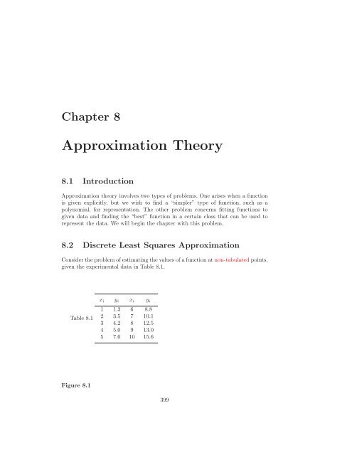
8.2 Discrete Least Squares Approximation 

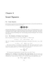
Consider the problem of estimating the values of a function at non-tabulated points, 

given the experimental data in Table 8.1. 

Table 8.1 

x i y i x i y i 

1 1.3 6 8.8 

2 3.5 7 10.1 

3 4.2 8 12.5 

4 5.0 9 13.0 

5 7.0 10 15.6 

Figure 8.1 

399

400 CHAPTER 8. APPROXIMATION THEORY 

y 

16 

14 

12 

10 

8 

6 

4 

2 

2 4 6 8 10 

x 

Interpolation requires a function that assumes the value of y i at x i for each 

i =1,2,...,10. Figure 8.1 on the following page shows a graph of the values in 

Table 8.1. From this graph, it appears that the actual relationship between x and 

y is linear. However, it is likely that no line precisely fits the data, because of 

errors in the data. In this case, it is unreasonable to require that the approximating 

function agree exactly with the given data; in fact, such a function would introduce 

oscillations that should not be present. For example, the graph of the ninth-degree 

interpolating polynomial for the data shown in Figure 8.2 is obtained using Maple 

with the commands 

>p:=interp([1,2,3,4,5,6,7,8,9,10],[1.3,3.5,4.2,5.0,7.0,8.8,10.1, 

12.5,13.0,15.6],x); 

>plot({p},x=1..10); 

Figure 8.2

8.2. DISCRETE LEAST SQUARES APPROXIMATION 401 

y 

16 

14 

12 

10 

8 

6 

4 

2 

2 4 6 8 10 

x 

This polynomial is clearly a poor predictor of information between a number of the 

data points. 

A better approach for a problem of this type would be to find the “best” (in 

some sense) approximating line, even if it did not agree precisely with the data at 

the points. 

Let a 1 x i + a 0 denote the ith value on the approximating line and y i the ith 

given y-value. Then, assuming that there are no errors in the x-values in the data, 

|y i − (a 1 x i + a 0 )| gives a measure for the error at the ith point when we use this 

approximating line. The problem of finding the equation of the best linear approximation 

in the absolute sense requires that values of a 0 and a 1 be found to minimize 

E ∞ (a 0 ,a 1 ) = max 

1≤i≤10 {|y i − (a 1 x i + a 0 )|}. 

This is commonly called a minimax problem and cannot be handled by elementary 

techniques. Another approach to determining the best linear approximation involves 

finding values of a 0 and a 1 to minimize 

E 1 (a 0 ,a 1 )= 

10∑ 

i=1 

|y i − (a 1 x i + a 0 )| . 

This quantity is called the absolute deviation. To minimize a function of two 

variables, we need to set its partial derivatives to zero and simultaneously solve the 

resulting equations. In the case of the absolute deviation, we would need to find a 0 

and a 1 with 

0= ∂ 

∂a 0 

10∑ 

i=1 

|y i − (a 1 x i + a 0 )| and 0 = ∂ 

∂a 1 

10∑ 

i=1 

|y i − (a 1 x i + a 0 )| .


The difficulty with this procedure is that the absolute-value function is not differentiable 

at zero, and solutions to this pair of equations cannot necessarily be 

obtained. 

The least squares approach to this problem involves determining the best 

approximating line when the error involved is the sum of the squares of the differences 

between the y-values on the approximating line and the given y-values. 

Hence, constants a 0 and a 1 must be found that minimize the total least squares 

error: 

E 2 (a 0 ,a 1 )= 

10∑ 

i=1 

|y i − (a 1 x i + a 0 )| 2 = 

10∑ 

i=1 

(y i − (a 1 x i + a 0 )) 2 . 

The least squares method is the most convenient procedure for determining best 

linear approximations, and there are also important theoretical considerations that 

favor this method. The minimax approach generally assigns too much weight to a 

bit of data that is badly in error, whereas the absolute deviation method does not 

give sufficient weight to a point that is badly out of line. The least squares approach 

puts substantially more weight on a point that is out of line with the rest of the 

data but will not allow that point to dominate the approximation. 

The general problem of fitting the best least squares line to a collection of data 

{(x i ,y i )} m i=1 involves minimizing the total error 

E 2 (a 0 ,a 1 )= 

m∑ 

(y i − (a 1 x i + a 0 )) 2 

i=1 

with respect to the parameters a 0 and a 1 . For a minimum to occur, we need 

0= ∂ 

∂a 0 

m 

∑ 

i=1 

(y i − (a 1 x i − a 0 )) 2 =2 

m∑ 

(y i − a 1 x i − a 0 )(−1) 

i=1 

and 

0= ∂ 

∂a 1 

m 

∑ 

i=1 

(y i − (a 1 x i + a 0 )) 2 =2 

m∑ 

(y i − a 1 x i − a 0 )(−x i ) 

i=1 

These equations simplify to the normal equations 

∑ m 

a 0 

i=1 

x i + a 1 

m 

∑ 

The solution to this system is as follows. 

m∑ 

∑ m m∑ 

x 2 i = x i y i and a 0 · m + a 1 x i = y i . 

i=1 i=1 

i=1 i=1


[Linear Least Squares] 

The linear least squares solution for a given collection of data {(x i ,y i )} m i=1 

has the form y = a 1 x + a 0 , where 

and 

a 0 = 

(∑ m 

) ∑ m 

i=1 x2 i ( 

i=1 y i) − ( ∑ m 

i=1 x iy i )( ∑ m 

i=1 x i) 

m ( ∑ m 

i=1 x2 i ) − (∑ m 

i=1 x i) 2 

a 1 = m (∑ m 

i=1 x iy i ) − ( ∑ m 

i=1 x i)( ∑ m 

i=1 y i) 

m ( ∑ m 

i=1 x2 i ) − (∑ m 

i=1 x i) 2 . 

EXAMPLE 1 

Consider the data presented in Table 8.1. To find the least squares line approximating 

this data, extend the table as shown in the third and fourth columns of 

Table 8.2, and sum the columns. 

Table 8.2 

x i y i x 2 i x i y i P (x i )=1.538x i − 0.360 

1 1.3 1 1.3 1.18 

2 3.5 4 7.0 2.72 

3 4.2 9 12.6 4.25 

4 5.0 16 20.0 5.79 

5 7.0 25 35.0 7.33 

6 8.8 36 52.8 8.87 

7 10.1 49 70.7 10.41 

8 12.5 64 100.0 11.94 

9 13.0 81 117.0 13.48 

10 15.6 100 156.0 15.02 

55 81.0 385 572.4 E = ∑ 10 

i=1 (y i − P (x i )) 2 ≈ 2.34 

Solving the normal equations produces 

a 0 = 

385(81) − 55(572.4) 

10(572.4) − 55(81) 

10(385) − (55) 2 = −0.360 and a 1 = 

10(385) − (55) 2 =1.538. 

So P (x) =1.538x − 0.360. The graph of this line and the data points are shown 

in Figure 8.3. The approximate values given by the least squares technique at the 

data points are in the final column in Table 8.2. 

Figure 8.3


y 

16 

14 

12 

10 

8 

6 

y 5 1.538x 2 0.360 

4 

2 

2 4 6 8 10 

x 

The problem of approximating a set of data, {(x i ,y i ) | i =1, 2,...,m}, with an 

algebraic polynomial 

P n (x) =a n x n + a n−1 x n−1 + ···+ a 1 x + a 0 

of degree n


EXAMPLE 2 

Fit the data in the first two rows of Table 8.3 with the discrete least squares 

polynomial of degree 2. For this problem, n =2,m = 5, and the three normal 

equations are 

5a 0 + 2.5a 1 + 1.875a 2 = 8.7680, 

2.5a 0 + 1.875a 1 + 1.5625a 2 = 5.4514, 

1.875a 0 + 1.5625a 1 + 1.3828a 2 = 4.4015. 

Table 8.3 

i 1 2 3 4 5 

x i 0 0.25 0.50 0.75 1.00 

y i 1.0000 1.2840 1.6487 2.1170 2.7183 

P (x i ) 1.0051 1.2740 1.6482 2.1279 2.7129 

y i − P (x i ) −0.0051 0.0100 0.0004 −0.0109 0.0054 

We can solve this linear system using Maple. We first define the equations 

>eq1:=5*a0+2.5*a1+1.875*a2=8.7680; 

>eq2:=2.5*a0+1.875*a1+1.5625*a2=5.4514; 

>eq3:=1.875*a0+1.5625*a1+1.3828*a2=4.4015; 

To solve the system we enter 

>solve({eq1,eq2,eq3},{a0,a1,a2}); 

which gives, with Digits set to 5, 

a 0 =1.0051, a 1 =0.86468, and a 2 =0.84316. 

Thus, the least squares polynomial of degree 2 fitting the preceding data is 

P 2 (x) =1.0051 + 0.86468x +0.84316x 2 , whose graph is shown in Figure 8.4. At the 

given values of x i , we have the approximations shown in Table 8.3. 

Figure 8.4


y 

2 

1 

y 5 1.0051 1 0.86468x 1 0.84316x 2 

0.25 0.50 0.75 1.00 

x 

The total error, 

5∑ 

(y i − P (x i )) 2 =2.76 × 10 −4 , 

i=1 

is the least that can be obtained by using a polynomial of degree at most 2.


EXERCISE SET 8.2 

1. Compute the linear least squares polynomial for the data of Example 2. 

2. Compute the least squares polynomial of degree 2 for the data of Example 1 

and compare the total error E 2 for the two polynomials. 

3. Find the least squares polynomials of degrees 1, 2, and 3 for the data in the 

following table. Compute the error E 2 in each case. Graph the data and the 

polynomials. 

x i 1.0 1.1 1.3 1.5 1.9 2.1 

y i 1.84 1.96 2.21 2.45 2.94 3.18 

4. Find the least squares polynomials of degrees 1, 2, and 3 for the data in the 

following table. Compute the error E 2 in each case. Graph the data and the 

polynomials. 

x i 0 0.15 0.31 0.5 0.6 0.75 

y i 1.0 1.004 1.031 1.117 1.223 1.422 

5. Given the following data 

x i 4.0 4.2 4.5 4.7 5.1 5.5 5.9 6.3 6.8 7.1 

y i 102.56 113.18 130.11 142.05 167.53 195.14 224.87 256.73 299.50 326.72 

(a) Construct the least squares polynomial of degree 1 and compute the 

error. 

(b) Construct the least squares polynomial of degree 2 and compute the 

error. 

(c) Construct the least squares polynomial of degree 3 and compute the 

error. 

6. Repeat Exercise 5 for the following data. 

x i 0.2 0.3 0.6 0.9 1.1 1.3 1.4 1.6 

y i 0.050446 0.098426 0.33277 0.72660 1.0972 1.5697 1.8487 2.5015


7. Hooke’s law states that when a force is applied to a spring constructed of 

uniform material, the length of the spring is a linear function of the force that 

is applied, as shown in the accompanying figure. 

l 

14 

12 

10 

8 

E 

l 

k(l 2 E) 5 F(l) 

6 

4 

2 

2 

4 

6 

F 

(a) Suppose that E =5.3 in. and that measurements are made of the length 

l in inches for applied weights F (l) in pounds, as given in the following 

table. Find the least squares approximation for k. 

F (l) 

l 

2 7.0 

4 9.4 

6 12.3 

(b) Additional measurements are made, giving the following additional data. 

Use these data to compute a new least squares approximation for k. 

Which of (a) or (b) best fits the total experimental data? 

F (l) l 

3 8.3 

5 11.3 

8 14.4 

10 15.9


8. To determine a relationship between the number of fish and the number of 

species of fish in samples taken for a portion of the Great Barrier Reef, P. Sale 

and R. Dybdahl [SD] fit a linear least squares polynomial to the following 

collection of data, which were collected in samples over a 2-year period. Let 

x be the number of fish in the sample and y be the number of species in the 

sample and determine the linear least squares polynomial for these data. 

x y x y x y 

13 11 29 12 60 14 

15 10 30 14 62 21 

16 11 31 16 64 21 

21 12 36 17 70 24 

22 12 40 13 72 17 

23 13 42 14 100 23 

25 13 55 22 130 34 

9. The following table lists the college grade-point averages of 20 mathematics 

and computer science majors, together with the scores that these students 

received on the mathematics portion of the ACT (American College Testing 

Program) test while in high school. Plot these data, and find the equation of 

the least squares line for this data. Do you think that the ACT scores are a 

reasonable predictor of college grade-point averages? 

ACT Grade-point ACT Grade-point 

Score Average Score Average 

28 3.84 29 3.75 

25 3.21 28 3.65 

28 3.23 27 3.87 

27 3.63 29 3.75 

28 3.75 21 1.66 

33 3.20 28 3.12 

28 3.41 28 2.96 

29 3.38 26 2.92 

23 3.53 30 3.10 

27 2.03 24 2.81


8.3 Continuous Least Squares Approximation 

Suppose f ∈ C[a, b] and we want a polynomial of degree at most n, 

to minimize the error 

P n (x) =a n x n + a n−1 x n−1 + ···+ a 1 x + a 0 = 

E(a 0 ,a 1 ,...,a n )= 

∫ b 

a 

(f(x) − P n (x)) 2 dx = 

∫ b 

a 

n∑ 

a k x k , 

k=0 

( 

f(x) − 

) 2 n∑ 

a k x k dx. 

A necessary condition for the numbers a 0 , a 1 ,...,a n to minimize the total error 

E is that 

∂E 

(a 0 ,a 1 ,...,a n ) =0 foreachj =0, 1,...,n. 

∂a j 

We can expand the integrand in this expression to 

∫ b 

n∑ 

∫ b 

∫ ( 

b n 

) 2 

∑ 

E = (f(x)) 2 dx − 2 a k x k f(x) dx + a k x k dx, 

so 

a 

k=0 

∂E 

∂a j 

(a 0 ,a 1 ,...,a n ) = −2 

∫ b 

a 

a 

x j f(x) dx +2 

a 

k=0 

k=0 

n∑ 

∫ b 

a k x j+k dx. 

for each j =0,1,...,n. Setting these to zero and rearranging, we obtain the (n+1) 

linear normal equations 

k=0 

a 

n∑ 

∫ b 

a k x j+k dx = 

∫ b 

k=0 

a 

a 

x j f(x) dx, 

for each j =0, 1,...,n, 

which must be solved for the n + 1 unknowns a 0 ,a 1 ,...,a n . The normal equations 

have a unique solution provided that f ∈ C[a, b]. 

EXAMPLE 1 Find the least squares approximating polynomial of degree 2 for the function f(x) = 

sin πx on the interval [0, 1]. 

The normal equations for P 2 (x) =a 2 x 2 + a 1 x + a 0 are 

∫ 1 ∫ 1 ∫ 1 

a 0 1 dx + a 1 xdx+ a 2 x 2 dx = 

0 

0 

0 

∫ 1 ∫ 1 ∫ 1 

a 0 xdx+ a 1 x 2 dx + a 2 x 3 dx = 

0 

0 

0 

∫ 1 ∫ 1 ∫ 1 

a 0 x 2 dx + a 1 x 3 dx + a 2 x 4 dx = 

0 

0 

0 

∫ 1 

0 

∫ 1 

0 

∫ 1 

0 

sin πx dx, 

x sin πx dx, 

x 2 sin πx dx.

8.3. CONTINUOUS LEAST SQUARES APPROXIMATION 411 

Performing the integration yields 

a 0 + 1 2 a 1 + 1 3 a 2 = 2 π , 1 

2 a 0 + 1 3 a 1 + 1 4 a 2 = 1 π , 1 

3 a 0 + 1 4 a 1 + 1 5 a 2 = π2 − 4 

π 3 . 

These three equations in three unknowns can be solved to obtain 

a 0 = 12π2 − 120 

720 − 60π2 

π 3 ≈−0.050465 and a 1 = −a 2 = 

π 3 ≈ 4.12251. 

Consequently, the least squares polynomial approximation of degree 2 for f(x) = 

sin πx on [0, 1] is P 2 (x) =−4.12251x 2 +4.12251x − 0.050465. (See Figure 8.5.) 

Figure 8.5 

y 

1.0 

f (x) 5 sin px 

0.8 

0.6 

P 2 (x) 

0.4 

0.2 

0.2 0.4 0.6 0.8 1.0 

x 

Example 1 illustrates the difficulty in obtaining a least squares polynomial approximation. 

An (n +1)× (n + 1) linear system for the unknowns a 0 ,...,a n must 

be solved, and the coefficients in the linear system are of the form 

∫ b 

a 

x j+k dx = bj+k+1 − a j+k+1 

. 

j + k +1 

The matrix in the linear system is known as a Hilbert matrix, whichisaclassic 

example for demonstrating round-off error difficulties. 

Another disadvantage to the technique used in Example 1 is similar to the 

situation that occurred when the Lagrange polynomials were first introduced in 

Section 3.2. We often don’t know the degree of the approximating polynomial that 

is most appropriate, and the calculations to obtain the best nth-degree polynomial 

do not lessen the amount of work required to obtain the best polynomials of higher


degree. Both disadvantages are overcome by resorting to a technique that reduces 

the n + 1 equations in n + 1 unknowns to n + 1 equations, each of which contains 

only one unknown. This simplifies the problem to one that can be easily solved, 

but the technique requires some new concepts. 

The set of functions {φ 0 ,φ 1 ,...,φ n } is said to be linearly independent on 

[a, b] if, whenever 

c 0 φ 0 (x)+c 1 φ 1 (x)+···+ c n φ n (x) = 0 

for all x ∈ [a, b], 

we have c 0 = c 1 = ···= c n = 0. Otherwise the set of functions is said to be linearly 

dependent. 

Linearly independent sets of functions are basic to our discussion and, since the 

functions we are using for approximations are polynomials, the following result is 

fundamental. 

[Linearly Independent Sets of Polynomials] 

If φ j (x), for each j =0,1,...,n, is a polynomial of degree j, then {φ 0 ,...,φ n } 

is linearly independent on any interval [a, b]. 

The situation illustrated in the following example demonstrates a fact that holds 

in a much more general setting. Let ∏ n 

be the set of all polynomials of degree 

at most n. If{φ 0 (x),φ 1 (x),...,φ n (x)} is any collection of linearly independent 

polynomials in ∏ n , then each polynomial in ∏ n 

can be written uniquely as a linear 

combination of {φ 0 (x),φ 1 (x),...,φ n (x)}. 

EXAMPLE 2 

Let φ 0 (x) =2,φ 1 (x) =x − 3, and φ 2 (x) =x 2 +2x + 7. Then {φ 0 ,φ 1 ,φ 2 } is linearly 

independent on any interval [a, b]. Suppose Q(x) =a 0 +a 1 x+a 2 x 2 .We will show that 

there exist constants c 0 , c 1 ,andc 2 such that Q(x) =c 0 φ 0 (x)+c 1 φ 1 (x)+c 2 φ 2 (x). 

Note first that 

1= 1 2 φ 0(x), x = φ 1 (x)+3=φ 1 (x)+ 3 2 φ 0(x), 

and 

( 

x 2 = φ 2 (x) − 2x − 7=φ 2 (x) − 2 φ 1 (x)+ 3 ) ( ) 1 

2 φ 0(x) − 7 

2 φ 0(x) 

= φ 2 (x) − 2φ 1 (x) − 13 2 φ 0(x). 

Hence, 

( ) ( 

1 

Q(x) = a 0 

2 φ 0(x) + a 1 φ 1 (x)+ 3 ) ( 

2 φ 0(x) + a 2 

= 

φ 2 (x) − 2φ 1 (x) − 13 

2 φ 0(x) 

( 1 

2 a 0 + 3 2 a 1 − 13 2 a 2) 

φ 0 (x)+(a 1 − 2a 2 )φ 1 (x)+a 2 φ 2 (x), 

so any quadratic polynomial can be expressed as a linear combination of φ 0 (x),φ 1 (x), 

and φ 2 (x). 

)


To discuss general function approximation requires the introduction of the notions 

of weight functions and orthogonality. An integrable function w is called a 

weight function on the interval I if w(x) ≥ 0 for all x in I, but w is not identically 

zero on any subinterval of I. 

The purpose of a weight function is to assign varying degrees of importance to 

approximations on certain portions of the interval. For example, the weight function 

w(x) = 

1 

√ 

1 − x 

2 

places less emphasis near the center of the interval (−1, 1) and more emphasis when 

|x| is near 1 (see Figure 8.6). This weight function will be used in the next section. 

Figure 8.6 

w(x) 

1 

21 

1 

x 

Suppose {φ 0 ,φ 1 ,...,φ n } is a set of linearly independent functions on [a, b], w 

is a weight function for [a, b], and, for f ∈ C[a, b], a linear combination 

is sought to minimize the error 

E(a 0 ,...,a n )= 

P (x) = 

∫ b 

a 

n∑ 

a k φ k (x) 

k=0 

( 

w(x) f(x) − 

2 n∑ 

a k φ k (x)) 

dx. 

This problem reduces to the situation considered at the beginning of this section 

in the special case when w(x) ≡ 1andφ k (x) =x k for each k =0,1,...,n. 

The normal equations associated with this problem are derived from the fact 

that for each j =0,1,...,n, 

0= ∂E 

∂a j 

(a 0 ,...,a n )=2 

∫ b 

a 

k=0 

( 

w(x) f(x) − 

The system of normal equations can be written 

∫ b 

a 

w(x)f(x)φ j (x) dx = 

) 

n∑ 

a k φ k (x) φ j (x) dx. 

k=0 

n∑ 

∫ b 

a k w(x)φ k (x)φ j (x) dx, 

k=0 

a 

for each j =0, 1,...,n.


If the functions φ 0 , φ 1 ,...,φ n can be chosen so that 

∫ b 

a 

w(x)φ k (x)φ j (x) dx = 

{ 

0, when j ≠ k, 

α k > 0, when j = k, 

(8.1) 

for some positive numbers α 0 , α 1 , ..., α n , then the normal equations reduce to 

∫ b 

a 

∫ b 

w(x)f(x)φ j (x) dx = a j w(x)[φ j (x)] 2 dx = a j α j 

for each j =0,1,...,n, and are easily solved as 

a j = 1 ∫ b 

w(x)f(x)φ j (x) dx. 

α j 

a 

Hence the least squares approximation problem is greatly simplified when the functions 

φ 0 ,φ 1 ,...,φ n are chosen to satisfy Eq. (8.1). 

The set of functions {φ 0 ,φ 1 ,...,φ n } is said to be orthogonal for the interval 

[a, b] with respect to the weight function w if for some positive numbers α 0 , α 1 ,..., 

α n , 

∫ { 

b 

0, when j ≠ k, 

w(x)φ j (x)φ k (x) dx = 

α k > 0, when j = k. 

a 

If, in addition, α k =1foreachk =0, 1,...,n, the set is said to be orthonormal. 

This definition, together with the remarks preceding it, implies the following. 

a 

[Least Squares for Orthogonal Functions] 

If {φ 0 ,φ 1 ,...,φ n } is an orthogonal set of functions on an interval [a, b] with 

respect to the weight function w, then the least squares approximation to f 

on [a, b] with respect to w is 

P (x) = 

n∑ 

a k φ k (x), 

k=0 

where 

∫ b 

a 

a k = 

w(x)φ k(x)f(x) dx 

∫ b 

a w(x)(φ k(x)) 2 dx 

= 1 ∫ b 

w(x)φ k (x)f(x) dx. 

α k a 

The next result, which is based on the Gram-Schmidt process, describes a recursive 

procedure for constructing orthogonal polynomials on [a, b] with respect to 

a weight function w.


[Recursive Generation of Orthogonal Polynomials] 

The set of polynomials {φ 0 (x),φ 1 (x),...,φ n (x)} defined in the following way 

is linearly independent and orthogonal on [a, b] with respect to the weight 

function w. 

φ 0 (x) ≡ 1, φ 1 (x) =x − B 1 , 

where 

and when k ≥ 2, 

where 

B 1 = 

∫ b 

a xw(x)(φ 0(x)) 2 dx 

∫ b 

a w(x)(φ 0(x)) 2 dx , 

φ k (x) =(x − B k )φ k−1 (x) − C k φ k−2 (x), 

∫ b 

a 

B k = 

xw(x)(φ k−1(x)) 2 dx 

∫ b 

a w(x)(φ k−1(x)) 2 dx 

∫ b 

a 

and C k = 

xw(x)φ k−1(x)φ k−2 (x) dx 

∫ b 

a w(x)(φ . 

k−2(x)) 2 dx 

Moreover, for any polynomial Q k (x) of degree kB3:=int(x*(x^2-1/3)^2,x=-1..1)/int((x^2-1/3)^2,x=-1..1); 

>C3:=int(x*(x^2-1/3)*x,x=-1..1)/int(x^2,x=-1..1);


gives B 3 =0andC 3 = 4 15 .Thus, 

P 3 (x) =xP 2 (x) − 4 

15 P 1(x) =x 3 − 1 3 x − 4 15 x = x3 − 3 5 x. 

The next two Legendre polynomials are P 4 (x) = x 4 − 6 7 x2 + 3 35 and P 5(x) = 

x 5 − 10 9 x3 + 5 

21x. Figure 8.7 shows the graphs of these polynomials. In general, we 

have, for each n ≥ 1, the recursive relationship 

P n+1 (x) =xP n (x) − 

n2 

4n 2 − 1 P n−1(x). (8.2) 

Figure 8.7 

P n (x) 

1 

P 1 (x) 

21 

0.5 

P 2 (x) 

P 3 (x) 

P 4 (x) 

P 5 (x) 

1 

x 

20.5 

21



1. Find the linear least squares polynomial approximation to f(x) on the indicated 

interval in each case. 

(a) f(x) =x 2 +3x +2,[0, 1]; (b) f(x) =x 3 ,[0, 2]; 

(c) f(x) = 1 x ,[1, 3]; (d) f(x) =e x ,[0, 2]; 

(e) f(x) = 1 2 cos x + 1 3 sin 2x, [0, 1]; (f) f(x) =x ln x, [1, 3]. 

2. Find the least squares polynomial approximation of degree 2 to the functions 

and intervals in Exercise 1. 

3. Find the linear least squares polynomial approximation on the interval [−1, 1] 

for the following functions. 

(a) f(x) =x 2 − 2x +3 

(c) f(x) = 1 

x +2 

(b) f(x) =x 3 

(d) f(x) =e x 

(e) f(x) = 1 2 cos x + 1 3 sin 2x (f) f(x) =ln(x +2) 

4. Find the least squares polynomial approximation of degree 2 on the interval 

[−1, 1] for the functions in Exercise 3. 

5. Compute the error E for the approximations in Exercise 3. 

6. Compute the error E for the approximations in Exercise 4. 

7. Use the Gram-Schmidt process to construct φ 0 (x), φ 1 (x), φ 2 (x), and φ 3 (x) 

for the following intervals. 

(a) [0, 1] 

(b) [0, 2] (c) [1, 3] 

8. Repeat Exercise 1 using the results of Exercise 7. 

9. Repeat Exercise 2 using the results of Exercise 7. 

10. Use the Gram-Schmidt procedure to calculate L 1 , L 2 ,andL 3 , where {L 0 (x), 

L 1 (x), L 2 (x), L 3 (x)} is an orthogonal set of polynomials on (0, ∞) with respect 

to the weight functions w(x) =e −x and L 0 (x) ≡ 1. The polynomials 

obtained from this procedure are called the Laguerre polynomials.


11. Use the Laguerre polynomials calculated in Exercise 10 to compute the least 

squares polynomials of degree 1, 2, and 3 on the interval (0, ∞) with respect 

to the weight function w(x) =e −x for the following functions. 

(a) f(x) =x 2 

(c) f(x) =x 3 

(b) f(x) =e−x 

(d) f(x) =e −2x 

12. Show that if {φ 0 ,φ 1 ,...,φ n } is an orthogonal set of functions on [a, b] with respect 

to the weight function w, then {φ 0 ,φ 1 ,...,φ n } is a linearly independent 

set. 

13. Suppose {φ 0 (x),φ 1 (x),...,φ n (x)} is a linearly independent set in ∏ n . Show 

that for any element Q(x) ∈ ∏ n there exist unique constants c 0,c 1 ,...,c n 

such that 

n∑ 

Q(x) = c k φ k (x). 

k=o

8.4. CHEBYSHEV POLYNOMIALS 419 

8.4 Chebyshev Polynomials 

The Chebyshev polynomials {T n (x)} are orthogonal on (−1, 1) with respect to 

the weight function w(x) =(1− x 2 ) −1/2 . Although they can be derived by the 

method in the previous section, it is easier to give a definition and then show that 

they are the polynomials that satisfy the required orthogonality properties. 

For x ∈ [−1, 1], define 

T n (x) =cos(n arccos x) for each n ≥ 0. 

It is not obvious from this definition that T n (x) isanth degree polynomial in x, 

but we will now show that it is. First note that 

T 0 (x) = cos 0 = 1 and T 1 (x) = cos(arccos x) =x. 

For n ≥ 1 we introduce the substitution θ = arccos x to change this equation to 

T n (x) =T n (θ(x)) ≡ T n (θ) =cos(nθ), 

where θ ∈ [0,π]. 

A recurrence relation is derived by noting that 

T n+1 (θ) =cos(nθ + θ) =cos(nθ)cosθ − sin(nθ)sinθ 

and 

T n−1 (θ) =cos(nθ − θ) =cos(nθ)cosθ +sin(nθ)sinθ. 

Adding these equations gives 

T n+1 (θ)+T n−1 (θ) =2cos(nθ)cosθ. 

Returning to the variable x and solving for T n+1 (x) we have, for each n ≥ 1, 

T n+1 (x) =2cos(n arccos x) · x − T n−1 (x) =2T n (x) · x − T n−1 (x). 

Since T 0 (x) andT 1 (x) are both polynomials in x, T n+1 (x) will be a polynomial in 

x for each n. 

[Chebyshev Polynomials] 

T 0 (x) =1, 

T 1 (x) =x, 

and, for n ≥ 1, T n+1 (x) is the polynomial of degree n + 1 given by 

T n+1 (x) =2xT n (x) − T n−1 (x).


The recurrence relation implies that T n (x) is a polynomial of degree n, andit 

has leading coefficient 2 n−1 , when n ≥ 1. The next three Chebyshev polynomials 

are 

and 

T 2 (x) =2xT 1 (x) − T 0 (x) =2x 2 − 1, 

T 3 (x) =2xT 2 (x) − T 1 (x) =4x 3 − 3x, 

T 4 (x) =2xT 3 (x) − T 2 (x) =8x 4 − 8x 2 +1. 

The graphs of T 1 , T 2 , T 3 ,andT 4 are shown in Figure 8.8. Notice that each of 

the graphs is symmetric to either the origin or the y-axis, and that each assumes a 

maximum value of 1 and a minimum value of −1 on the interval [−1, 1]. 

Figure 8.8 

T 3 (x) 

T n (x) 

1 

T 4 (x) 

T 1 (x) 

21 

1 

x 

21 

T 2 (x) 

To show the orthogonality of the Chebyshev polynomials, consider 

∫ 1 

∫ 1 

∫ 

T n (x)T m (x) 

1 

cos(n arccos x)cos(m arccos x) 

w(x)T n (x)T m (x) dx = √ dx = 

√ dx. 

−1 

−1 1 − x 

2 

−1 

1 − x 

2 

Reintroducing the substitution θ = arccos x gives 

1 

dθ = −√ dx 

1 − x 

2


and 

∫ 1 

−1 


√ 

1 − x 

2 

dx = − 

Suppose n ≠ m. Since 

we have 

∫ 1 

−1 


√ 

1 − x 

2 

∫ 0 

π 

cos(nθ)cos(mθ) dθ = 

∫ π 

cos(nθ)cos(mθ) = 1 (cos(n + m)θ +cos(n − m)θ) , 

2 

∫ π 

0 

cos(nθ)cos(mθ) dθ. 

dx = 1 cos((n + m)θ) dθ + 1 cos((n − m)θ) dθ 

2 0 

2 0 

[ 

] π 

1 

= 

2(n + m) sin ((n + m)θ)+ 1 

2(n − m) sin(n − m)θ =0. 

0 

By a similar technique, it can also be shown that 

∫ π 

∫ 1 

−1 

(T n (x)) 2 

√ 

1 − x 

2 dx = π 2 

for each n ≥ 1. 

One of the important results about the Chebyshev polynomials concerns their 

zeros and extrema. These are easily verified by substitution into the polynomials 

and their derivatives. 

[Zeros and Extrema of Chebyshev Polynomials] 

The Chebyshev polynomial T n (x), of degree n ≥ 1, has n simple zeros in 

[−1, 1] at 

( ) 2k − 1 

x k =cos 

2n π for each k =1, 2,...,n. 

Moreover, T n assumes its absolute extrema at 

( ) kπ 

x ′ k =cos with T n (x ′ 

n 

k)=(−1) k for each k =0, 1,...,n. 

The monic Chebyshev polynomial (polynomial with leading coefficient 1), ˜T n (x), 

is derived from the Chebyshev polynomial, T n (x), by dividing by the leading coefficient, 

2 n−1 , when n ≥ 1. So 

˜T 0 (x) =1, and ˜Tn (x) =2 1−n T n (x) for each n ≥ 1. 

These polynomials satisfy the recurrence relation 

˜T 2 (x) =x ˜T 1 (x) − 1 2 ˜T 0 (x); 

˜Tn+1 (x) =x ˜T n (x) − 1 4 ˜T n−1 (x),


for each n ≥ 2. Because ˜T n is a multiple of T n , the zeros of ˜T n also occur at 

( ) 2k − 1 

x k =cos 

2n π for each k =1, 2,...,n, 

and the extreme values of ˜T n occur at 

( ) kπ 

x ′ k =cos with ˜Tn (x ′ 

n 

k)= (−1)k 

2 n−1 for each k =0, 1, 2,...,n. 

Let ˜Π n denote the set of all monic polynomials of degree n. The following 

minimization property distinguishes the polynomials ˜T n (x) from the other members 

of ˜Π n . 

[Minimum Property of Monic Chebyshev Polynomials] The polynomial ˜T n (x), 

when n ≥ 1, has the property that 

1 

= max 

2n−1 | ˜T n (x)| ≤ max |P n(x)| for all P n ∈ ˜Π n . 

x∈[−1,1] x∈[−1,1] 

Moreover, equality can occur only if P n = ˜T n . 

This result is used to answer the question of where to place interpolating nodes 

to minimize the error in Lagrange interpolation. The error form for the Lagrange 

polynomial applied to the interval [−1, 1] states that if x 0 ,...,x n are distinct numbers 

in the interval [−1, 1] and if f ∈ C n+1 [−1, 1], then, for each x ∈ [−1, 1], a 

number ξ(x) existsin(−1, 1) with 

f(x) − P (x) = f (n+1) (ξ(x)) 

(x − x 0 ) ···(x − x n ), 

(n + 1)! 

where P (x) is the Lagrange interpolating polynomial. Suppose that we want to 

minimize this error for all values of x in [−1, 1]. We have no control over ξ(x), so 

to minimize the error by shrewd placement of the nodes x 0 ,...,x n is equivalent to 

choosing x 0 ,...,x n to minimize the quantity 

|(x − x 0 )(x − x 1 ) ···(x − x n )| 

throughout the interval [−1, 1]. 

Since (x − x 0 )(x − x 1 ) ···(x − x n ) is a monic polynomial of degree n +1, the 

minimum is obtained when 

(x − x 0 )(x − x 1 ) ···(x − x n )= ˜T n+1 (x). 

When x k is chosen to be the (k + 1)st zero of ˜T n+1 , that is, when x k is 

x k+1 =cos 

2k +1 

2(n +1) π,


the maximum value of |(x − x 0 )(x − x 1 ) ···(x − x n )| is minimized. Since 

max ∣ ˜T n+1 (x) ∣ = 1 

this also implies that 

x∈[−1,1] 

1 

2 n = max 

x∈[−1,1] |(x − x 1)(x − x 2 ) ···(x − x n+1 )| 

≤ 

2 n 

max |(x − x 0)(x − x 1 ) ···(x − x n )| , 

x∈[−1,1] 

for any choice of x 0 , x 1 ,...,x n in the interval [−1, 1]. 

[Minimizing Lagrange Interpolation Error] 

If P (x) is the interpolating polynomial of degree at most n with nodes at the 

roots of T n+1 (x), then, for any f ∈ C n+1 [−1, 1], 

max |f(x) − P (x)| ≤ 1 

x∈[−1,1] 2 n (n + 1)! 

max 

x∈[−1,1] 

∣ 

∣f (n+1) (x) ∣ . 

The technique for choosing points to minimize the interpolating error can be 

easily extended to a general closed interval [a, b] by using the change of variable 

˜x = 1 ((b − a)x + a + b) 

2 

to transform the numbers x k in the interval [−1, 1] into the corresponding numbers 

in the interval [a, b], as shown in the next example. 

EXAMPLE 1 

Let f(x) =xe x on [0, 1.5]. Two interpolation polynomials of degree at most 3 will 

be constructed. First, the equally spaced nodes x 0 =0,x 1 =0.5, x 2 =1, and 

x 3 =1.5 are used. The methods in Section 3.2 give this interpolating po1ynomial 

as 

P 3 (x) =1.3875x 3 +0.057570x 2 +1.2730x. 

For the second interpolating polynomial we will use the nodes given by the zeros 

of the Chebyshev polynomial ˜T 4 .Firstweshift these zeros x k = cos((2k +1)/8)π, 

for k =0,1,2,and3,from[−1, 1] to [0, 1.5], using the linear transformation 

˜x k = 1 2 ((1.5 − 0)x k +(1.5 + 0)) =0.75 + 0.75x k 

to obtain 

˜x 0 =1.44291, ˜x 1 =1.03701, ˜x 2 =0.46299, and ˜x 3 =0.05709. 

For these nodes, the interpolation polynomial of degree at most 3 is 

˜P 3 (x) =1.3811x 3 +0.044652x 2 +1.3031x − 0.014352.


Table 8.4 

x f(x) =xe x P 3 (x) |xe x − P 3 (x)| ˜P3 (x) |xe x − ˜P 3 (x)| 

0.15 0.1743 0.1969 0.0226 0.1868 0.0125 

0.25 0.3210 0.3435 0.0225 0.3358 0.0148 

0.35 0.4967 0.5121 0.0154 0.5064 0.0097 

0.65 1.245 1.233 0.0120 1.231 0.0140 

0.75 1.588 1.572 0.0160 1.571 0.0170 

0.85 1.989 1.976 0.0130 1.974 0.0150 

1.15 3.632 3.650 0.0180 3.644 0.0120 

1.25 4.363 4.391 0.0280 4.382 0.0190 

1.35 5.208 5.237 0.0290 5.224 0.0160 

Table 8.4 lists various values of x, together with the values of f(x), P 3 (x), and 

˜P 3 (x). Although the error using P 3 (x) is less than using ˜P 3 (x) near the middle of the 

table, the maximum error involved with using ˜P 3 (x), which is ˜P 3 (1.25) = 0.019, is 

considerably less than the maximium error using P 3 (x), which is P 3 (1.35) = 0.029. 

(See Figure 8.9.) 

Figure 8.9 

y 

6 

5 

4 

, 

P 3 (x) 

y 5 xe x 

3 

2 

1 

0.5 1.0 1.5 

x



1. Use the zeros of ˜T 3 to construct an interpolating polynomial of degree 2 for 

the following functions on the interval [−1, 1]. 

(a) f(x) =e x 

(b) f(x) =sinx 

(c) f(x) =ln(x +2) (d) f(x) =x 4 

2. Find a bound for the maximum error of the approximation in Exercise 1 on 

the interval [−1, 1]. 


the functions in Exercise 1. 

4. Repeat Exercise 2 for the approximations computed in Exercise 3. 

5. Use the zeros of ˜T 3 and transformations of the given interval to construct an 

interpolating polynomial of degree 2 for the following functions. 

(a) f(x) = 1 x ,[1, 3] (b) f(x) =e −x ,[0, 2] 

(c) f(x) = 1 2 cos x + 1 3 sin 2x, [0, 1] (d) f(x) =x ln x, [1, 3] 


the functions in Exercise 5. 

7. Show that for any positive integers i and j with i>jwe have 

T i (x)T j (x) = 1 2 [T i+j(x)+T i−j (x)]. 

8. Show that for each Chebyshev polynomial T n (x) wehave 

∫ 1 

−1 

[T n (x)] 2 

√ 

1 − x 

2 dx = π 2 .


8.5 Rational Function Approximation 

The class of algebraic polynomials has some distinct advantages for use in approximation. 

There is a sufficient number of polynomials to approximate any continuous 

function on a closed interval to within an arbitrary tolerance, polynomials are easily 

evaluated at arbitrary values, and the derivatives and integrals of polynomials exist 

and are easily determined. The disadvantage of using polynomials for approximation 

is their tendency for oscillation. This often causes error bounds in polynomial 

approximation to significantly exceed the average approximation error, since error 

bounds are determined by the maximum approximation error. We now consider 

methods that spread the approximation error more evenly over the approximation 

interval. 

A rational function r of degree N has the form 

r(x) = p(x) 

q(x) , 

where p(x) andq(x) are polynomials whose degrees sum to N. 

Since every polynomial is a rational function (simply let q(x) ≡ 1), approximation 

by rational functions gives results with no greater error bounds than approximation 

by polynomials. However, rational functions whose numerator and denominator 

have the same or nearly the same degree generally produce approximation 

results superior to polynomial methods for the same amount of computational effort. 

Rational functions have the added advantage of permitting efficient approximation 

of functions with infinite discontinuities near the interval of approximation. 

Polynomial approximation is generally unacceptable in this situation. 

Suppose r is a rational function of degree N = n + m of the form 

r(x) = p(x) 

q(x) = p 0 + p 1 x + ···+ p n x n 

q 0 + q 1 x + ···+ q m x m 

that is used to approximate a function f on a closed interval I containing zero. For 

r to be defined at zero requires that q 0 ≠ 0. In fact, we can assume that q 0 =1, 

for if this is not the case we simply replace p(x) byp(x)/q 0 and q(x) byq(x)/q 0 . 

Consequently, there are N + 1 parameters q 1 , q 2 ,...,q m , p 0 , p 1 ,...,p n available for 

the approximation of f by r. 

The Padé approximation technique chooses the N + 1 parameters so that 

f (k) (0) = r (k) (0) for each k =0,1,...,N.Padé approximation is the extension 

of Taylor polynomial approximation to rational functions. In fact, when n = N and 

and m =0,thePadé approximation is the Nth Taylor polynomial expanded about 

zero—that is, the Nth Maclaurin polynomial. 

Consider the difference 

f(x) − r(x) =f(x) − p(x) f(x)q(x) − p(x) 

= = f(x) ∑ m 

i=0 q ix i − ∑ n 

i=0 p ix i 

q(x) q(x) 

q(x) 

and suppose f has the Maclaurin series expansion f(x) = ∑ ∞ 

i=0 a ix i . Then 

∑ ∞ 

i=0 

f(x) − r(x) = 

a ix i ∑ m 

i=0 q ix i − ∑ n 

i=0 p ix i 

. (8.3) 

q(x)

8.5. RATIONAL FUNCTION APPROXIMATION 427 

The object is to choose the constants q 1 , q 2 ,...,q m and p 0 , p 1 ,...,p n so that 

f (k) (0) − r (k) (0) = 0 

for each k =0, 1,...,N. 

This is equivalent to f −r having a zero of multiplicity N +1 at 0. As a consequence, 

we choose q 1 , q 2 ,...,q m and p 0 , p 1 ,...,p n so that the numerator on the right side 

of Eq. (8. 3 ), 

(a 0 + a 1 x + ···)(1 + q 1 x + ···+ q m x m ) − (p 0 + p 1 x + ···+ p n x n ), 

has no terms of degree less than or equal to N. 

To make better use of summation notation we define p n+1 = p n+2 = ···= p N = 

0andq m+1 = q m+2 = ···= q N = 0. The coefficient of x k is then 

( k∑ 

) 

a i q k−i − p k , 

i=0 

and the rational function for Padé approximation results from the solution of the 

N + 1 linear equations 

k∑ 

a i q k−i = p k , 

i=0 

k =0, 1,...,N 

in the N + 1 unknowns q 1 ,q 2 ,...,q m ,p 0 ,p 1 ,...,p n . 

The Padé technique can be implemented using the program PADEMD81. 

EXAMPLE 1 

To find the Padé approximation of degree 5 with n =3andm =2to 

e −x = 

∞∑ (−1) i 

x i . 

i! 

i=0 

requires choosing p 0 , p 1 , p 2 , p 3 , q 1 ,andq 2 so that the coefficients of x k for k =0, 

1,...,5 are zero in the expression 

(1 ···) − x + x2 

2 − x3 (1+q1 

6 + x + q 2 x 2) − ( p 0 + p 1 x + p 2 x 2 + p 3 x 3) . 

Expanding and collecting terms produces 

x 5 : − 1 + 1 

120 24 q 1 − 1 6 q 2 = 0; x 2 1 

: − q 1 + q 2 = p 2 ; 

2 

x 4 1 1 

: − 

24 6 q 1 + 1 2 q 2 = 0; x 1 : −1 + q 1 = p 1 ; 

x 3 : − 1 1 

+ 

6 2 q 1 − q 2 = p 3 ; x 0 : 1 = p 0 . 

To solve the linear system in Maple we use the following:


>eq1:=-1+q1=p1; 

>eq2:=1/2-q1+q2=p2; 

>eq3:=-1/6+1/2*q1-q2=p3; 

>eq4:=1/24-1/6*q1+1/2*q2=0; 

>eq5:=-1/120+1/24*q1-1/6*q2=0; 

>solve({eq1,eq2,eq3,eq4,eq5},{q1,q2,p1,p2,p3}); 

which gives 

p 0 =1, p 1 = − 3 5 , p 2 = 3 

20 , p 3 = − 1 

60 , q 1 = 2 5 , and q 2 = 1 20 . 

So the Padé approximation is 

r(x) = 1 − 3 5 x + 3 20 x2 − 1 

60 x3 

1+ 2 5 x + 1 . 

20 x2 

Maple can also be used to compute a Padé approximation directly. We first 

compute the Maclaurin series with the call 

>series(exp(-x),x); 

to obtain 

1 − x + 1 2 x2 − 1 6 x3 + 1 

24 x4 − 1 

120 x5 + O(x 6 ) 

The Padé approximation with n =3andm = 2 is computed using the command 

>g:=convert(%,ratpoly,3,2); 

where the % refers to the result of the preceding calculation, that is, the Maple 

statement series(exp(-x),x), which gives the Maclaurin series for e −x . The result 

is 

g := 1 − 3 5 x + 3 

20 x2 − 1 60 x3 

1+ 2 5 x + 1 . 

20 x2 

We can then compute the approximations, such as g(0.8), by entering 

>evalf(subs(x=0.8,g)); 

to get .4493096647. 

Table 8.5 lists values of r(x) andP 5 (x), the fifth Maclaurin polynomial. The 

Padé approximation is clearly superior in this example.


Table 8.5 

x e −x P 5 (x) |e −x − P 5 (x)| r(x) |e −x − r(x)| 

0.2 0.81873075 0.81873067 8.64 × 10 −8 0.81873075 7.55 × 10 −9 

0.4 0.67032005 0.67031467 5.38 × 10 −6 0.67031963 4.11 × 10 −7 

0.6 0.54881164 0.54875200 5.96 × 10 −5 0.54880763 4.00 × 10 −6 

0.8 0.44932896 0.44900267 3.26 × 10 −4 0.44930966 1.93 × 10 −5 

1.0 0.36787944 0.36666667 1.21 × 10 −3 0.36781609 6.33 × 10 −5 

It is interesting to compare the number of arithmetic operations required for 

calculations of P 5 (x) andr(x) in Example 1. Using nested multiplication, P 5 (x) 

canbeexpressedas 

(((( 

P 5 (x) = − 1 

120 x + 1 ) 

x − 1 ) 

x + 1 ) ) 

x − 1 x +1. 

24 6 2 

Assuming that the coefficients of 1,x,x 2 ,x 3 ,x 4 , and x 5 are represented as decimals, 

a single calculation of P 5 (x) in nested form requires five multiplications and 

five additions/subtractions. Using nested multiplication, r(x) is expressed as 

(( 

− 

1 

60 

r(x) = 

x + ) 3 

20 x − 

3 

5) 

x +1 

( 1 

20 x + ) 2 , 

5 x +1 

so a single calculation of r(x) requires five multiplications, five additions/subtractions, 

and one division. Hence, computational effort appears to favor the polynomial approximation. 

However, by reexpressing r(x) by continued division, we can write 

or 

r(x) = 1 − 3 5 x + 3 

20 x2 − 1 

60 x3 

1+ 2 5 x + 1 

20 x2 

= − 1 3 x3 +3x 2 − 12x +20 

x 2 +8x +20 

= − 1 3 x + 17 ( 

− 

152 

3 + 3 x − ) 

280 

3 

x 2 +8x +20 

= − 1 3 x + 17 3 + − 152 

( 

3 

) 

x 2 +8x+20 

x+ 35 

19 

r(x) =− 1 3 x + 17 

152 

3 − ⎛ 3 

⎞ 

⎝ x+ 117 

3125 

19 + 361 

(x+ 35 ⎠ 

19 ) 

Written in this form, a single calculation of r(x) requires one multiplication, five 

addition/subtractions, and two divisions. If the amount of computation required for 

division is approximately the same as for multiplication, the computational effort 

.


required for an evaluation of P 5 (x) significantly exceeds that required for an evaluation 

of r(x). Expressing a rational function approximation in this form is called 

continued-fraction approximation. This is a classical approximation technique of 

current interest because of its computational efficiency. It is, however, a specialized 

technique—one we will not discuss further. 

Although the rational function approximation in Example 1 gave results superior 

to the polynomial approximation of the same degree, the approximation has a 

wide variation in accuracy; the approximation at 0.2 is accurate to within 8 × 

10 −9 , whereas, at 1.0, the approximation and the function agree only to within 

7 × 10 −5 .This accuracy variation is expected, because the Padé approximation is 

based on a Taylor polynomial representation of e −x , and the Taylor representation 

has a wide variation of accuracy in [0.2, 1.0]. 

To obtain more uniformly accurate rational function approximations, we use the 

set of Chebyshev polynomials, a class that exhibits more uniform behavior. The 

general Chebyshev rational function approximation method proceeds in the same 

manner as Padé approximation, except that each x k term in the Padé approximation 

is replaced by the kth-degree Chebyshev polynomial T k . An introduction to this 

technique and more detailed references can be found in Burden and Faires [BF], 

pp. 523–527.



1. Determine all Padé approximations for f(x) =e 2x of degree 2. Compare the 

results at x i =0.2i, fori =1, 2, 3, 4, 5, with the actual values f(x i ). 

2. Determine all Padé approximations for f(x) =x ln(x+1) of degree 3. Compare 

the results at x i =0.2i, fori =1, 2, 3, 4, 5, with the actual values f(x i ). 

3. Determine the Padé approximation of degree 5 with n =2andm =3for 

f(x) =e x . Compare the results at x i =0.2i, fori =1, 2, 3, 4, 5, with those 

from the fifth Maclaurin polynomial. 

4. Repeat Exercise 3 using instead the Padé approximation of degree 5 with 

n =3andm =2. 

5. Determine the Padé approximation of degree 6 with n = m =3forf(x) = 

sin x. Compare the results at x i =0.1i, fori =0, 1,...,5, with the exact 

results and with the results of the sixth Maclaurin polynomial. 

6. Determine the Padé approximations of degree 6 with (a) n =2,m =4and 

(b) n =4,m =2forf(x) =sinx. Compare the results at each x i to those 

obtained in Exercise 5. 

7. Table 8.5 lists results of the Padé approximation of degree 5 with n =3and 

m = 2, the fifth Maclaurin polynomial, and the exact values of f(x) =e −x 

when x i =0.2i, fori =1, 2, 3, 4, and 5. Compare these results with those 

produced from the other Padé approximations of degree 5. 

(a) n =0,m=5 

(c) n =3,m=2 

(b) n =1,m=4 

(d) n =4,m=1 

8. Express the following rational functions in continued-fraction form. 

(a) x2 +3x +2 

x 2 − x +1 

(c) 2x3 − 3x 2 +4x − 5 

x 2 +2x +4 

(b) 

(d) 

4x 2 +3x − 7 

2x 3 + x 2 − x +5 

2x 3 + x 2 − x +3 

3x 3 +2x 2 − x +1 

9. To accurately approximate sin x and cos x for inclusion in a mathematical 

library, we first restrict their domains. Given a real number x, divide by π to 

obtain the relation 

|x| = Mπ + s, where M is an integer and |s| ≤ π 2 .


(a) Show that sin x =sgn(x)(−1) M sin s. 

(b) Construct a rational approximation to sin s using n = m = 4. Estimate 

the error when 0 ≤|s| ≤ π 2 . 

(c) Design an implementation of sin x using parts (a) and (b). 

(d) Repeat part (c) for cos x using the fact that cos x =sin(x + π 2 ). 

10. To accurately approximate f(x) =e x for inclusion in a mathematical library, 

we first restrict the domain of f. Given a real number x, divide by ln √ 10 to 

obtain the relation 

x = M ln √ 10 + s, 

where M is an integer and s is a real number satisfying |s| ≤ 1 2 ln √ 10. 

(a) Show that e x = e s 10 M/2 . 

(b) Construct a rational function approximation for e s using n = m =3. 

Estimate the error when 0 ≤|s| ≤ 1 2 ln √ 10. 

(c) Design an implementation of e x using the results of part (a) and (b) 

and the approximations 

1 

ln √ 10 =0.8685889638 and √ 10 = 3.162277660.

8.6. TRIGONOMETRIC POLYNOMIAL APPROXIMATION 433 

8.6 Trigonometric Polynomial Approximation 

Trigonometric functions are used to approximate functions that have periodic behavior, 

functions with the property that for some constant T , f(x + T )=f(x) 

for all x. We can generally transform the problem so that T =2π and restrict the 

approximation to the interval [−π, π]. 

For each positive integer n, the set T n of trigonometric polynomials of degree 

less than or equal to n is the set of all linear combinations of {φ 0 ,φ 1 ,...,φ 2n−1 }, 

where 

φ 0 (x) = 1 2 , 

φ k (x) = cos kx, 

for each k =1, 2,...,n, 

and 

φ n+k (x) =sinkx, for each k =1, 2,...,n− 1. 

(Some sources include an additional function in the set, φ 2n (x) =sin nx.) 

The set {φ 0 ,φ 1 ,...,φ 2n−1 } is orthogonal on [−π, π] with respect to the weight 

function w(x) ≡ 1.This follows from a demonstration similar to that which shows 

that the Chebyshev polynomials are orthogonal on [−1, 1]. For example, if k ≠ j 

and j ≠0, 

∫ π 

−π 

The trigonometric identity 

φ n+k (x)φ j (x) dx = 

∫ π 

−π 

sin kx cos jxdx. 

sin kx cos jx = 1 2 sin(k + j)x + 1 sin(k − j)x 

2 

can now be used to give 

∫ π 

φ n+k (x)φ j (x) dx = 1 ∫ π 

(sin(k + j)x +sin(k − j)x) dx 

−π 2 −π 

= 1 [ ] π − cos(k + j)x cos(k − j)x 

− =0, 

2 k + j k − j 

−π 

since cos(k + j)π =cos(k + j)(−π) and cos(k − j)π =cos(k − j)(−π). The result 

also holds when k = j, for in this case we have sin(k − j)x = sin 0 = 0. 

Showing orthogonality for the other possibilities from {φ 0 ,φ 1 ,...,φ 2n−1 } is similar 

and uses the appropriate trigonometric identities from the collection 

sin jxcos kx = 1 (sin(j + k)x +sin(j − k)x), 

2 

sin jxsin kx = 1 (cos(j − k)x − cos(j + k)x), 

2 

cos jxcos kx = 1 (cos(j + k)x +cos(j − k)x), 

2


to convert the products into sums. 

Given f ∈ C[−π, π], the continuous least squares approximation by functions 

in T n is defined by 

S n (x) = 1 2n−1 

2 a ∑ 

0 + a k φ k (x), 

k=1 

where 

a k = 1 π 

∫ π 

−π 

f(x)φ k (x) dx for each k =0, 1,...,2n − 1. 

The limit of S n (x) asn →∞is called the Fourier series of f(x). Fourier series are 

used to describe the solution of various ordinary and partial-differential equations 

that occur in physical situations. 

EXAMPLE 1 

To determine the trigonometric polynomial from T n that approximates 

f(x) =|x| 

for − π


y 

p 

q 

y 5 uxu 

4 4 

y 5 S 3 (x) 5 q 2 cos x 2 cos 3x 

p 9p 

4 

y 5 S 1 (x) 5 S 2 (x) 5 q 2 p cos x 

y 5 S 0 (x) 5 q 

2p 

2q 

q 

p 

x 

The Fourier series for f(x) =|x| is 

S(x) = lim 

n→∞ S n(x) = π 2 + 2 π 

∞∑ 

k=1 

(−1) k − 1 

k 2 

cos kx. 

Since | cos kx| ≤1 for every k and x, the series converges and S(x) exists for all 

real numbers x. 

There is a discrete analog to Fourier series that is useful for the least squares 

approximation and interpolation of large amounts of data when the data are given at 

equally spaced points. Suppose that a collection of 2m paired data points {(x j ,y j )} 2m−1 

j=0 

is given, with the first elements in the pairs equally partitioning a closed interval. 

For convenience, we assume that the interval is [−π, π] and that, as shown in Figure 

8.11, 

( j 

x j = −π + π for each j =0, 1,...,2m − 1. 

m) 

If this were not the case, a linear transformation could be used to change the data 

into this form. 

Figure 8.11 

2p 5 x 0 

0 5 x m 

p 5 x 2m 

The goal is to determine the trigonometric polynomial, S n (x), in T n that minimizes 

E(S n )= 

2m−1 

∑ 

j=0 

(y j − S n (x j )) 2 .


That is, we want to choose the constants a 0 ,a 1 ,...,a n and b 1 ,b 2 ,...,b n−1 to minimize 

the total error 

[ ( 

2m−1 

∑ 

n−1 

2 

a 0 

E(S n )= y j − 

2 + a ∑ 

n cos nx j + (a k cos kx j + b k sin kx j ))] 

. 

j=0 

The determination of the constants is simplified by the fact that the set is 

orthogonal with respect to summation over the equally spaced points {x j } 2m−1 

j=0 in 

[−π, π]. By this we mean that, for each k ≠ l, 

2m−1 

∑ 

j=0 

k=1 

φ k (x j )φ l (x j )=0. 

The orthogonality follows from the fact that if r and m are positive integers with 

r


and the transformed data are of the form 

{( ( 

z j ,f 1+ z ))} 9 

j 

. 

π j=0 

Consequently, the least squares trigonometric polynomial is 

where 

and 

S 3 (z) = a 0 

2 + a 3 cos 3z + 

a k = 1 5 

b k = 1 5 

9∑ ( 

f 

j=0 

9∑ ( 

f 

j=0 

1+ z j 

π 

1+ z j 

π 

2∑ 

(a k cos kz + b k sin kz), 

k=1 

Evaluating these sums produces the approximation 

) 

cos kz j , for k =0, 1, 2, 3, 

) 

sin kz j , for k =1, 2. 

S 3 (z) = 0.76201 + 0.77177 cos z +0.017423 cos 2z +0.0065673 cos 3z 

− 0.38676 sin z +0.047806 sin 2z. 

Converting back to the variable x gives 

S 3 (x) = 0.76201 + 0.77177 cos π(x − 1) + 0.017423 cos 2π(x − 1) 

+0.0065673 cos 3π(x − 1) 

− 0.38676 sin π(x − 1) + 0.047806 sin 2π(x − 1). 

Table 8.6 lists values of f(x) andS 3 (x). 

Table 8.6 

x f(x) S 3 (x) |f(x) − S 3 (x)| 

0.125 0.26440 0.24060 2.38 × 10 −2 

0.375 0.84081 0.85154 1.07 × 10 −2 

0.625 1.36150 1.36248 9.74 × 10 −4 

0.875 1.61282 1.60406 8.75 × 10 −3 

1.125 1.36672 1.37566 8.94 × 10 −3 

1.375 0.71697 0.71545 1.52 × 10 −3 

1.625 0.07909 0.06929 9.80 × 10 −3 

1.875 −0.14576 −0.12302 2.27 × 10 −2



1. Find the continuous least squares trigonometric polynomial S 2 (x) forf(x) = 

x 2 on [−π, π]. 

2. Find the continuous least squares trigonometric polynomial S n (x) forf(x) = 

x on [−π, π]. 

3. Find the continuous least squares trigonometric polynomial S 3 (x) forf(x) = 

e x on [−π, π]. 

4. Find the general continuous least squares trigonometric polynomial S n (x) for 

f(x) =e x on [−π, π]. 

5. Find the general continuous least squares trigonometric polynomial S n (x) for 

{ 

0, if −π


12. Show that for any continuous even function f defined on the interval [−a, a], 

we have ∫ a 

−a f(x) dx =2∫ a 

f(x) dx. 

0 

13. Show that the functions φ 0 (x) =1/2,φ 1 (x) = cos x,...,φ n (x) = cos nx, φ n+1 (x) = 

sin x,...,φ 2n−1 (x) =sin(n − 1)x,are orthogonal on [−π, π] with respect to 

w(x) ≡ 1. 

14. In Example 1 the Fourier series was determined for f(x) = |x|. Use this 

series and the assumption that it represents f at zero to find the value of the 

convergent infinite series 

∞∑ 1 

(2k +1) 2 . 

k=0


8.7 Fast Fourier Transforms 

The interpolatory trigonometric polynomial on the 2m data points {(x j ,y j )} 2m−1 

j=0 is 

the least squares polynomial from T m for this collection of points. The least squares 

trigonometric polynomial S n (x), when n

8.7. FAST FOURIER TRANSFORMS 441 

The method described by Cooley and Tukey is generally known as the Fast 

Fourier Transform (FFT) method and led to a revolution in the use of interpolatory 

trigonometric polynomials. The method consists of organizing the problem 

so that the number of data points being used can be easily factored, particularly 

into powers of 2. 

The relationship between the number of data points 2m and the degree of the 

trigonometric polynomial used in the fast Fourier transform procedure allows some 

notational simplification. The nodes are given, for each j =0, 1,...,2m − 1, by 

( j 

x j = −π + π 

m) 

and the coefficients, for each k =0, 1,...,m,as 

a k = 1 m 

2m−1 

∑ 

j=0 

y j cos kx j and b k = 1 m 

2m−1 

∑ 

j=0 

y j sin kx j . 

For notational convenience, b 0 and b m have been added to the collection, but both 

are zero and do not contribute to the sum. 

Instead of directly evaluating the constants a k and b k , the fast Fourier transform 

procedure computes the complex coefficients c k in the formula 

where 

c k = 

2m−1 

∑ 

j=0 

F (x) = 1 m 

2m−1 

∑ 

k=0 

c k e ikx , 

y j e πijk/m , for each k =0, 1,...,2m − 1. (8.6) 

Once the constants c k have been determined, a k and b k can be recovered. To 

do this we need Euler’s formula, which states that for all real numbers z we have 

e iz =cosz + i sin z, 

where the complex number i satisfies i 2 = −1. Then, for each k =0, 1,...,m, 

1 

m c ke −iπk = 1 2m−1 

∑ 

y j e πijk/m e −iπk = 1 m 

m 

= 1 m 

j=0 

2m−1 

∑ 

j=0 

y j (cos kx j + i sin kx j ), 

2m−1 

∑ 

j=0 

y j e ik(−π+(πj/m)) 

so 

1 

m c ke −iπk = a k + ib k . 

The operation reduction feature of the fast Fourier transform results from calculating 

the coefficients c k in clusters. The following example gives a simple illustration 

of the technique.


EXAMPLE 1 Consider the construction of the trigonometric interpolating polynomial of degree 2 

for the data {(x 0 ,y 0 ), (x 1 ,y 1 ), (x 2 ,y 2 ), (x 3 ,y 3 )}, where m =2andx j = −π+(j/2)π 

for j =0, 1, 2, 3. The polynomial is given by 

S 2 (x) = a 0 + a 2 cos 2x 

+ a 1 cos x + b 1 sin x, 

2 

where the coefficients are 

a 0 = 1 2 (y 0 cos 0 + y 1 cos 0 + y 2 cos 0 + y 3 cos 0) = 1 2 (y 0 + y 1 + y 2 + y 3 ), 

a 1 = 1 2 (y 0 cos x 0 + y 1 cos x 1 + y 2 cos x 2 + y 3 cos x 3 ), 

a 2 = 1 2 (y 0 cos 2x 0 + y 1 cos 2x 1 + y 2 cos 2x 2 + y 3 cos 2x 3 ), 

b 1 = 1 2 (y 0 sin x 0 + y 1 sin x 1 + y 2 sin x 2 + y 3 sin x 3 ). 

Introducing the complex coefficients defined in Eq. (8. 6 )wehave 

c 0 = y 0 e 0 + y 1 e 0 + y 2 e 0 + y 3 e 0 , 

c 1 = y 0 e 0 + y 1 e πi/2 + y 2 e πi + y 3 e 3πi/2 , 

c 2 = y 0 e 0 + y 1 e πi + y 2 e 2πi + y 3 e 3πi , 

c 3 = y 0 e 0 + y 1 e 3πi/2 + y 2 e 3πi + y 3 e 9πi/2 , 

and a k + ib k = 1 2 e−kπi c k for k =0, 1, 2, 3. Thus 

a 0 = 1 2 Re(c 0), a 1 = 1 2 Re(c 1e −πi ), 

a 2 = 1 2 Re(c 2e −2πi ), b 1 = 1 2 Im(c 1e −πi ). 

If we let δ = e πi/2 we can rewrite the equations as the matrix equation 

⎡ ⎤ ⎡ 

⎤ ⎡ ⎤ 

c 0 1 1 1 1 y 0 

⎢ c 1 

⎥ 

⎣ c 2 

⎦ = ⎢ 1 δ δ 2 δ 3 

⎥ ⎢ y 1 

⎥ 

⎣ 1 δ 2 δ 4 δ 6 ⎦ ⎣ y 2 

⎦ . 

c 3 1 δ 3 δ 6 δ 9 y 3 

Since δ 4 =1,δ 5 = δ, δ 6 = δ 2 , δ 7 = δ 3 , δ 8 = δ 4 =1,δ 9 = δ 5 = δ, wehave 

⎡ ⎤ ⎡ 

⎤ ⎡ ⎤ 

c 0 1 1 1 1 y 0 

⎢ c 1 

⎥ 

⎣ c 2 

⎦ = ⎢ 1 δ δ 2 δ 3 

⎥ ⎢ y 1 

⎥ 

⎣ 1 δ 2 1 δ 2 ⎦ ⎣ y 2 

⎦ . 

c 3 1 δ 3 δ 2 δ y 3 

Factoring the matrix product gives 

⎡ ⎤ ⎡ 

⎤ ⎡ 

⎤ ⎡ 

c 0 1 1 0 0 1 1 0 0 

⎢ c 1 

⎥ 

⎣ c 2 

⎦ = ⎢ 0 0 1 1 

⎥ ⎢ 0 0 δ 3 δ 3 

⎥ ⎢ 

⎣ 1 δ 2 0 0 ⎦ ⎣ 1 δ 2 0 0 ⎦ ⎣ 

c 3 0 0 1 δ 2 0 0 1 δ 2 

1 0 0 0 

0 0 1 0 

0 δ 0 0 

0 0 0 δ 

⎤ 

⎥ 

⎦ 

⎡ 

⎢ 

⎣ 

y 0 

y 1 

y 2 

y 3 

⎤ 

⎥ 

⎦ ,


and since δ 2 = e πi =cosπ + i sin π = −1 wehave 

⎡ ⎤ ⎡ 

⎤ ⎡ 

c 0 1 1 0 0 1 1 0 0 

⎢ c 1 

⎥ 

⎣ c 2 

⎦ = ⎢ 0 0 1 1 

⎥ ⎢ 0 0 δ 3 δ 3 

⎣ 1 −1 0 0 ⎦ ⎣ 1 −1 0 0 

c 3 0 0 1 −1 0 0 1 −1 

⎤ 

⎥ 

⎦ 

⎡ 

⎢ 

⎣ 

1 0 0 0 

0 0 1 0 

0 δ 0 0 

0 0 0 δ 

Computing (c 0 ,c 1 ,c 2 ,c 3 ) t using the factored form requires 2 multiplications by δ, 

2byδ 3 ,and4byδ 2 = −1. In addition, each matrix multiplication requires 4 

additions. Hence we have a total of 8 multiplications and 4 additions. The original 

product required 16 multiplications and 12 additions. 

⎤ 

⎥ 

⎦ 

⎡ 

⎢ 

⎣ 

y 0 

y 1 

y 2 

y 3 

⎤ 

⎥ 

⎦ . 

In general, the number of multiplications is reduced from 4m 2 to 3m + m log 2 m 

when the fast Fourier transform is applied. In Example 2, we have m = 2 which 

reduced the number of multiplications from 4 · 2 2 =16to3· 2 + 2 log 2 2=8. 

This perhaps does not seem significant, but if the example had instead used m = 

128 points, it would have reduced the multiplications from 4 · 128 2 = 65536 to 

3 · 128 + 128 log 2 128 = 384 + 128 · 7 = 1280. 

The program FFTRNS82 performs the fast Fourier transform when m =2 p for 

some positive integer p. Modifications to the technique can be made when m takes 

other forms. 

EXAMPLE 2 

Let f(x) =x 4 −3x 3 +2x 2 −tan x(x−2). To determine the trigonometric interpolating 

polynomial of degree 4 for the data {(x j ,y j )} 7 j=0 where x j = j/4 andy j = f(x j ) 

requires a transformation of the interval [0, 2] to [−π, π]. The linear transformation 

is given by 

z j = π(x j − 1) 

so that the input data to the fast Fourier transform method is 

The interpolating polynomial in z is 

{ ( 

z j ,f 1+ z )} 7 

j 

. 

π j=0 

S 4 (z) = 0.761979 + 0.771841 cos z +0.0173037 cos 2z 

+0.00686304 cos 3z − 0.000578545 cos 4z 

− 0.386374 sin z +0.0468750 sin 2z − 0.0113738 sin 3z. 

The trigonometric polynomial S 4 (x) on[0, 2] is obtained by substituting z = 

π(x − 1) into S 4 (z). The graphs of y = f(x) andy = S 4 (x) areshowninFigure 

8.12. Values of f(x) andS 4 (x) are given in Table 8.7.


Table 8.7 

x f(x) S 4 (x) |f(x) − S 4 (x)| 

0.125 0.26440 0.25001 1.44 × 10 −2 

0.375 0.84081 0.84647 5.66 × 10 −3 

0.625 1.36150 1.35824 3.27 × 10 −3 

0.875 1.61282 1.61515 2.33 × 10 −3 

1.125 1.36672 1.36471 2.02 × 10 −3 

1.375 0.71697 0.71931 2.33 × 10 −3 

1.625 0.07909 0.07496 4.14 × 10 −3 

1.875 −0.14576 −0.13301 1.27 × 10 −2 

Figure 8.12 

y 

2 

1 

y 5 f (x) 

y 5 S 4 (x) 

1 2 

x



1. Determine the trigonometric interpolating polynomial S 2 (x) of degree 2 on 

[−π, π] for the following functions, and graph f(x) − S 2 (x). 

(a) f(x) =π(x − π) 

(c) f(x) =|x| 

(b) f(x) =x(π − x) 

(d) f(x) = 

{ 

−1, if −π ≤ x ≤ 0 

1, if 0


8.8 Survey of Methods and Software 

In this chapter we have considered approximating data and functions with elementary 

functions. The elementary functions used were polynomials, rational functions, 

and trigonometric polynomials. We considered two types of approximations, discrete 

and continuous. Discrete approximations arise when approximating a finite set of 

data with an elementary function. Continuous approximations are used when the 

function to be approximated is known. 

Discrete least squares techniques are recommended when the function is specified 

by giving a set of data that may not exactly represent the function. Least 

squares fit of data can take the form of a linear or other polynomial approximation 

or even an exponential form. These approximations are computed by solving sets 

of normal equations, as given in Section 8.2. 

If the data are periodic, a trigonometric least squares fit may be appropriate. 

Because of the orthonormality of the trigonometric basis functions, the least squares 

trigonometric approximation does not require the solution of a linear system. For 

large amounts of periodic data, interpolation by trigonometric polynomials is also 

recommended. An efficient method of computing the trigonometric interpolating 

polynomial is given by the fast Fourier transform. 

When the function to be approximated can be evaluated at any required argument, 

the approximations seek to minimize an integral instead of a sum. The 

continuous least squares polynomial approximations were considered in Section 

8.3. Efficient computation of least squares polynomials lead to orthonormal sets 

of polynomials, such as the Legendre and Chebyshev polynomials. Approximation 

by rational functions was studied in Section 8.5, where Padé approximation as a 

generalization of the Maclaurin polynomial was presented. This method allows a 

more uniform method of approximation than polynomials. Continuous least squares 

approximation by trigonometric functions was discussed in Section 8.6, especially 

as it relates to Fourier series. 

The IMSL Library and the NAG Libraries provide subroutines for least squares 

approximation of data. The approximation can be by polynomials, cubic splines, 

or a users’ choice of basis functions. Chebyshev polynomials are also used in the 

constructions to minimize round-off error and enhance accuracy, and Fast Fourier 

transformations are available. 

The netlib library contains the subroutine polfit.f under the package slatec to 

compute the polynomial least squares approximation to a discrete set of points. 

The subroutine pvalue.f can be used to evaluate the polynomial from polfit.f and 

any of its derivatives at a given point. 

For further information on the general theory of approximation theory see Powell 

[Po], Davis [Da], or Cheney [Ch]. A good reference for methods of least squares is 

Lawson and Hanson [LH], and information about Fourier transforms can be found 

in Van Loan [Van] and in Briggs and Hanson [BH].

Chapter 8 Approximation Theory

Create successful ePaper yourself

Delete template?

Save as template?