Mathematica Tutorial: Unconstrained Optimization - Wolfram Research

Wolfram Mathematica ® Tutorial Collection 

UNCONSTRAINED OPTIMIZATION

For use with Wolfram Mathematica ® 7.0 and later. 

For the latest updates and corrections to this manual: 

visit reference.wolfram.com 

For information on additional copies of this documentation: 

visit the Customer Service website at www.wolfram.com/services/customerservice 

or email Customer Service at info@wolfram.com 

Comments on this manual are welcomed at: 

comments@wolfram.com 

Content authored by: 

Rob Knapp 

Printed in the United States of America. 

15 14 13 12 11 10 9 8 7 6 5 4 3 2 

©2008 Wolfram Research, Inc. 

All rights reserved. No part of this document may be reproduced or transmitted, in any form or by any means, 

electronic, mechanical, photocopying, recording or otherwise, without the prior written permission of the copyright 

holder. 

Wolfram Research is the holder of the copyright to the Wolfram Mathematica software system ("Software") described 

in this document, including without limitation such aspects of the system as its code, structure, sequence, 

organization, “look and feel,” programming language, and compilation of command names. Use of the Software unless 

pursuant to the terms of a license granted by Wolfram Research or as otherwise authorized by law is an infringement 

of the copyright. 

Wolfram Research, Inc. and Wolfram Media, Inc. ("Wolfram") make no representations, express, 

statutory, or implied, with respect to the Software (or any aspect thereof), including, without limitation, 

any implied warranties of merchantability, interoperability, or fitness for a particular purpose, all of 

which are expressly disclaimed. Wolfram does not warrant that the functions of the Software will meet 

your requirements or that the operation of the Software will be uninterrupted or error free. As such, 

Wolfram does not recommend the use of the software described in this document for applications in 

which errors or omissions could threaten life, injury or significant loss. 

Mathematica, MathLink, and MathSource are registered trademarks of Wolfram Research, Inc. J/Link, MathLM, 

.NET/Link, and webMathematica are trademarks of Wolfram Research, Inc. Windows is a registered trademark of 

Microsoft Corporation in the United States and other countries. Macintosh is a registered trademark of Apple 

Computer, Inc. All other trademarks used herein are the property of their respective owners. Mathematica is not 

associated with Mathematica Policy Research, Inc.

Contents 

Introduction . . . . . . . . . . . . . . . . . . . . . . . . . . . . . . . . . . . . . . . . . . . . . . . . . . . . . . . . . . . . . . . . . . . . . . . . 1 

Methods for Local Minimization 

Introduction . . . . . . . . . . . . . . . . . . . . . . . . . . . . . . . . . . . . . . . . . . . . . . . . . . . . . . . . . . . . . . . . . . . . 7 

Newton's Method . . . . . . . . . . . . . . . . . . . . . . . . . . . . . . . . . . . . . . . . . . . . . . . . . . . . . . . . . . . . . . . 8 

Quasi-Newton Methods . . . . . . . . . . . . . . . . . . . . . . . . . . . . . . . . . . . . . . . . . . . . . . . . . . . . . . . . . 15 

Gauss-Newton Methods . . . . . . . . . . . . . . . . . . . . . . . . . . . . . . . . . . . . . . . . . . . . . . . . . . . . . . . . . 18 

Nonlinear Conjugate Gradient Methods . . . . . . . . . . . . . . . . . . . . . . . . . . . . . . . . . . . . . . . . . 21 

Principal Axis Method . . . . . . . . . . . . . . . . . . . . . . . . . . . . . . . . . . . . . . . . . . . . . . . . . . . . . . . . . . . 23 

Methods for Solving Nonlinear Equations 

Introduction . . . . . . . . . . . . . . . . . . . . . . . . . . . . . . . . . . . . . . . . . . . . . . . . . . . . . . . . . . . . . . . . . . . . 25 

Newton’s Method . . . . . . . . . . . . . . . . . . . . . . . . . . . . . . . . . . . . . . . . . . . . . . . . . . . . . . . . . . . . . . . 25 

The Secant Method . . . . . . . . . . . . . . . . . . . . . . . . . . . . . . . . . . . . . . . . . . . . . . . . . . . . . . . . . . . . . 28 

Brent’s Method . . . . . . . . . . . . . . . . . . . . . . . . . . . . . . . . . . . . . . . . . . . . . . . . . . . . . . . . . . . . . . . . . 29 

Step Control 

Introduction . . . . . . . . . . . . . . . . . . . . . . . . . . . . . . . . . . . . . . . . . . . . . . . . . . . . . . . . . . . . . . . . . . . . 31 

Line Search Methods . . . . . . . . . . . . . . . . . . . . . . . . . . . . . . . . . . . . . . . . . . . . . . . . . . . . . . . . . . . . 32 

Trust Region Methods . . . . . . . . . . . . . . . . . . . . . . . . . . . . . . . . . . . . . . . . . . . . . . . . . . . . . . . . . . 39 

Setting Up Optimization Problems in Mathematica 

Specifying Derivatives . . . . . . . . . . . . . . . . . . . . . . . . . . . . . . . . . . . . . . . . . . . . . . . . . . . . . . . . . . 44 

Variables and Starting Conditions . . . . . . . . . . . . . . . . . . . . . . . . . . . . . . . . . . . . . . . . . . . . . . . 49 

Termination Conditions . . . . . . . . . . . . . . . . . . . . . . . . . . . . . . . . . . . . . . . . . . . . . . . . . . . . . . . . . 53 

Symbolic Evaluation . . . . . . . . . . . . . . . . . . . . . . . . . . . . . . . . . . . . . . . . . . . . . . . . . . . . . . . . . . . . 59 

UnconstrainedProblems Package 

Plotting Search Data . . . . . . . . . . . . . . . . . . . . . . . . . . . . . . . . . . . . . . . . . . . . . . . . . . . . . . . . . . . . 62 

Test Problems . . . . . . . . . . . . . . . . . . . . . . . . . . . . . . . . . . . . . . . . . . . . . . . . . . . . . . . . . . . . . . . . . . 65 

References . . . . . . . . . . . . . . . . . . . . . . . . . . . . . . . . . . . . . . . . . . . . . . . . . . . . . . . . . . . . . . . . . . . . . . . . . 71

Introduction to Unconstrained 

Optimization 

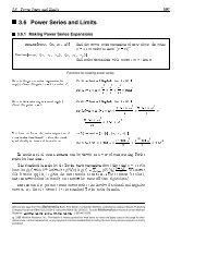
Mathematica has a collection of commands that do unconstrained optimization (FindMinimum 

and FindMaximum) and solve nonlinear equations (FindRoot) and nonlinear fitting problems 

(FindFit). All these functions work, in general, by doing a search, starting at some initial 

values and taking steps that decrease (or for FindMaximum, increase) an objective or merit 

function. 

The search process for FindMaximum is somewhat analogous to a climber trying to reach a 

mountain peak in a thick fog; at any given point, basically all that climbers know is their position, 

how steep the slope is, and the direction of the fall line. One approach is always to go 

uphill. As long as climbers go uphill steeply enough, they will eventually reach a peak, though it 

may not be the highest one. Similarly, in a search for a maximum, most methods are ascent 

methods where every step increases the height and stops when it reaches any peak, whether it 

is the highest one or not. 

The analogy with hill climbing can be reversed to consider descent methods for finding local 

minima. For the most part, the literature in optimization considers the problem of finding minima, 

and since this applies to most of the Mathematica commands, from here on, this documentation 

will follow that convention. 

For example, the function x sinHx + 1L is not bounded from below, so it has no global minimum, 

but it has an infinite number of local minima. 

In[1]:= 

This loads a package that contains some utility functions. 

2 Unconstrained Optimization 

This shows the steps taken by FindMinimum for the function x Sin@x + 1D starting at x = 0. 

In[3]:= FindMinimumPlot@x Sin@x + 1D, 8x, 0

Unconstrained Optimization 3 

This shows the steps taken by FindMinimum for the function x Sin@x + 1D starting at x = 7. 

In[5]:= FindMinimumPlot@x Sin@x + 1D, 8x, 7


The FindMinimumPlot command for two dimensions is similar to the one-dimensional case, but 

it shows the steps and evaluations superimposed on a contour plot of the function. In this 

example, it is apparent that FindMinimum needed to change direction several times to get to 

the local minimum. You may notice that the first step starts in the direction of steepest descent 

(i.e., perpendicular to the contour or parallel to the gradient). Steepest descent is indeed a 

possible strategy for local minimization, but it often does not converge quickly. In subsequent 

steps in this example, you may notice that the search direction is not exactly perpendicular to 

the contours. The search is using information from past steps to try to get information about 

the curvature of the function, which typically gives it a better direction to go. Another strategy, 

which usually converges faster, but can be more expensive, is to use the second derivative of 

the function. This is usually referred to as "Newton's" method. 

In[7]:= 

This shows the steps taken using Newton's method. 

FindMinimumPlot@Cos@x^2 - 3 yD + Sin@x^2 + y^2D, 88x, 1


For the most part, local minimization methods for a function f are based on a quadratic model 

q k HpL = f Hx k L + “ f Hx k L T p + 1 2 pT B k p. 

(1) 

The subscript k refers to the k th iterative step. In Newton's method, the model is based on the 

exact Hessian matrix, B k = “ 2 f Hx k L , but other methods use approximations to “ 2 f Hx k L, which are 

typically less expensive to compute. A trial step s k is typically computed to be the minimizer of 

the model, which satisfies the system of linear equations. 

B k s k 

= - “ f Hx k L 

If f is sufficiently smooth and x k is sufficiently close to a local minimum, then with B k = “ 2 f Hx k L, 

the sequence of steps x k+1 = s k + x k is guaranteed to converge to the local minimum. However, in 

a typical search, the starting value is rarely close enough to give the desired convergence. 

Furthermore, B k is often an approximation to the actual Hessian and, at the beginning of a 

search, the approximation is frequently quite inaccurate. Thus, it is necessary to provide additional 

control to the step sequence to improve the chance and rate of convergence. There are 

two frequently used methods for controlling the steps: line search and trust region methods. 

In a "line search" method, for each trial step s k found, a one-dimensional search is done along 

the direction of s k so that x k+1 = x k + a k s k . You could choose a k so that it minimizes f Hx k+1 L in this 

direction, but this is excessive, and with conditions that require that f Hx k+1 L decreases sufficiently 

in value and slope, convergence for reasonable approximations B k can be proven. Mathematica 

uses a formulation of these conditions called the Wolfe conditions. 

In a "trust region" method, a radius D k within which the quadratic model q k HpL in equation (1) is 

“trusted” to be reasonably representative of the function. Then, instead of solving for the unconstrained 

minimum of (1), the trust region method tries to find the constrained minimum of (1) 

with °p¥ § D k . If the x k are sufficiently close to a minimum and the model is good, then often the 

minimum lies within the circle, and convergence is quite rapid. However, near the start of a 

search, the minimum will lie on the boundary, and there are a number of techniques to find an 

approximate solution to the constrained problem. Once an approximate solution is found, the 

actual reduction of the function value is compared to the predicted reduction in the function 

value and, depending on how close the actual value is to the predicted, an adjustment is made 

for D k+1 .


For symbolic minimization of a univariate smooth function, all that is necessary is to find a point 

at which the derivative is zero and the second derivative is positive. In multiple dimensions, 

this means that the gradient vanishes and the Hessian needs to be positive definite. (If the 

Hessian is positive semidefinite, the point is a minimizer, but is not necessarily a strict one.) As 

a numerical algorithm converges, it is necessary to keep track of the convergence and make 

some judgment as to when a minimum has been approached closely enough. This is based on 

the sequence of steps taken and the values of the function, its gradient, and possibly its Hessian 

at these points. Usually, the Mathematica Find… functions will issue a message if they 

cannot be fairly certain that this judgment is correct. However, keep in mind that discontinuous 

functions or functions with rapid changes of scale can fool any numerical algorithm. 

When solving "nonlinear equations", many of the same issues arise as when finding a "local 

minimum". In fact, by considering a so-called merit function, which is zero at the root of the 

equations, it is possible to use many of the same techniques as for minimization, but with the 

advantage of knowing that the minimum value of the function is 0. It is not always advantageous 

to use this approach, and there are some methods specialized for nonlinear equations. 

Most examples shown will be from one and two dimensions. This is by no means because Mathematica 

is restricted to computing with such small examples, but because it is much easier to 

visually illustrate the main principles behind the theory and methods with such examples.


Methods for Local Minimization 

Introduction to Local Minimization 

The essence of most methods is in the local quadratic model 

q k HpL = f Hx k L + “ f Hx k L T p + 1 2 pT B k p 

that is used to determine the next step. The FindMinimum function in Mathematica has five 

essentially different ways of choosing this model, controlled by the method option. These methods 

are similarly used by FindMaximum and FindFit. 

"Newton" 

"QuasiNewton" 

"LevenbergMarquardt" 

"ConjugateGradient" 

use the exact Hessian or a finite difference approximation 

if the symbolic derivative cannot be computed 

use the quasi-Newton BFGS approximation to the Hessian 

built up by updates based on past steps 

a Gauss|Newton method for least-squares problems; the 

Hessian is approximated by J T J, where J is the Jacobian of 

the residual function 

a nonlinear version of the conjugate gradient method for 

solving linear systems; a model Hessian is never formed 

explicitly 

"PrincipalAxis" works without using any derivatives, not even the gradi - 

ent, by keeping values from past steps; it requires two 

starting conditions in each variable 

Basic method choices for FindMinimum. 

With Method -> Automatic, Mathematica uses the "quasi-Newton" method unless the problem 

is structurally a sum of squares, in which case the Levenberg|Marquardt variant of the "Gauss| 

Newton" method is used. When given two starting conditions in each variable, the "principal 

axis" method is used.


Newton's Method 

One significant advantage Mathematica provides is that it can symbolically compute derivatives. 

This means that when you specify Method -> "Newton" and the function is explicitly differentiable, 

the symbolic derivative will be computed automatically. On the other hand, if the function 

is not in a form that can be explicitly differentiated, Mathematica will use finite difference 

approximations to compute the Hessian, using structural information to minimize the number of 

evaluations required. Alternatively you can specify a Mathematica expression, which will give 

the Hessian with numerical values of the variables. 


In[1]:= 


When the gradient and Hessian are both computed using finite differences, the error in the 

Hessian may be quite large and it may be better to use a different method. In this case, 

FindMinimum does find the minimum quite accurately, but cannot be sure because of inadequate 

derivative information. Also, the number of function and gradient evaluations is much 

greater than in the example with the symbolic derivatives computed automatically because 

extra evaluations are required to approximate the gradient and Hessian, respectively. 

If it is possible to supply the gradient (or the function is such that it can be computed automatically), 

the method will typically work much better. You can give the gradient using the 

Gradient option, which has several ways you can "specify derivatives". 

This defines a function that returns the gradient for numerical values of x and y. 

In[5]:= 

g@x_ ?NumberQ, y_ ?NumberQD = Map@D@Cos@x^2 - 3 yD + Sin@x^2 + y^2D, ÒD &, 8x, y


this way depends on the function being convex, in which case the Hessian is always positive 

definite. It is common that a search will start at a location where this condition is violated, so 

the algorithm needs to take this possibility into account. 

Here is an example where the search starts near a local maximum. 

In[9]:= 

FindMinimumPlot@Cos@x^2 - 3 yD + Sin@x^2 + y^2D, 

88x, 1.2


modifies the Hessian by a diagonal matrix E k with entries large enough so that B k = “ 2 f Hx k L + E k is 

positive definite. Such methods are sometimes referred to as modified Newton methods. The 

modification to B k is done during the process of computing a Cholesky decomposition somewhat 

along the lines described in [GMW81], both for dense and sparse Hessians. The modification is 

only done if “ 2 f Hx k L is not positive definite. This decomposition method is accessible through 

LinearSolve if you want to use it independently. 

In[12]:= 

This computes the step using B 0 s 0 = -“ f Hx k L, where B 0 is determined as the Cholesky factors of 

the Hessian are being computed. 

LinearSolve@h@1.2, .5D, -g@1.2, .5D, 

Method Ø 8"Cholesky", "Modification" Ø "Minimal" 0. 

At machine precision, this does not always make a substantial difference since it is typical that 

most of the steps are spent getting near to the local minimum. However, if you want a root to 

extremely high precision, Newton's method is usually the best choice because of the rapid 

convergence. 

This computes a very high-precision solution using Newton's method. The precision is adaptively 

increased from machine precision (the precision of the starting point) to the maximal 

working precision of 100000 digits. Reap is used with Sow to save the steps taken. Counters 

are used to track and print the number of function evaluations and steps used. 

In[14]:= First@Timing@Block@8e = 0, s = 0


When the option WorkingPrecision -> prec is used, the default for the AccuracyGoal and 

PrecisionGoal is prec ê 2. Thus, this example should find the minimum to at least 50000 digits. 

This computes a symbolic solution for the position of the minimum which the search approaches. 

In[15]:= 

exact = 8x, y< ê. Last@Solve@8x^2 + y^2 ã 3 Pi ê 2, x^2 - 3 y ã -Pi


Note that typically the precision is roughly double the scale Ilog 10 

M of the error. For Newton's 

method this is appropriate since when the step is computed, the scale of the error will effectively 

double according to the quadratic convergence. 

FindMinimum always starts with the precision of the starting values you gave it. Thus, if you do 

not want it to use adaptive precision control, you can start with values, which are exact or have 

at least the maximum WorkingPrecision. 

This computes the solution using only precision 100000 throughout the computation. (Warning: 

this takes a very long time to complete.) 



In[20]:= 

This shows the steps taken by FindMinimum with a trust region Newton method for a Rosenbrock 

function. 

FindMinimumPlot@p, Method Ø 8"Newton", "StepControl" -> "TrustRegion"


Quasi-Newton Methods 

There are many variants of quasi-Newton methods. In all of them, the idea is to base the 

matrix B k in the quadratic model 

q k HpL = f Hx k L + “ f Hx k L T p + 1 2 pT B k p 

on an approximation of the Hessian matrix built up from the function and gradient values from 

some or all steps previously taken. 


In[1]:= 


The BFGS method is implemented such that instead of forming the model Hessian B k at each 

step, Cholesky factors L k such that L k .L T k = B k are computed so that only OIn 2 M operations are 

needed to solve the system B k s k = -“ f Hx k L [DS96] for a problem with n variables. 

For large-scale sparse problems, the BFGS method can be problematic because, in general, the 

Cholesky factors (or the Hessian approximation B k or its inverse) are dense, so the OIn 2 M memory 

and operations requirements become prohibitive compared to algorithms that take advantage 

of sparseness. The L-BFGS algorithm [NW99] forms an approximation to the inverse 

Hessian based on the last m past steps, which are stored. The Hessian approximation may not 

be as complete, but the memory and order of operations are limited to OHn mL for a problem with 

n variables. In Mathematica 5, for problems over 250 variables, the algorithm is switched automatically 

to L-BFGS. You can control this with the method option "StepMemory" -> m. With 

m = , the full BFGS method will always be used. Choosing an appropriate value of m is a tradeoff 

between speed of convergence and the work done per step. With m < 3, you are most likely 

better off using a "conjugate gradient" algorithm. 

In[3]:= 

This shows the same example function with the minimum computed using L-BFGS with m = 5. 

FindMinimumPlot@Cos@x^2 - 3 yD + Sin@x^2 + y^2D, 

88x, 1


°x k+1 - x * ¥ 

lim 

kØ °x k - x * ¥ = 0 

or, in other words, the steps keep getting smaller. However, for very high precision, this does 

not compare to the q-quadratic convergence rate of "Newton's" method. 

This shows the number of steps and function evaluations required to find the minimum to high 

precision for the problem shown. 



Gauss|Newton Methods 

For minimization problems for which the objective function is a sum of squares, 

m 

f HxL = 1 2 ‚ r j HxL 2 = 1 

j=1 

2 rHxL.rHxL, 

it is often advantageous to use the special structure of the problem. Time and effort can be 

saved by computing the residual function rHxL, and its derivative, the Jacobian JHxL. The Gauss| 

Newton method is an elegant way to do this. Rather than using the complete second-order 

Hessian matrix for the quadratic model, the Gauss|Newton method uses B k = J T k J k in (1) such 

that the step p k is computed from the formula 

J k T J k p k = - “ f k = - J k T r k , 

where J k = JHx k L, and so on. Note that this is an approximation to the full Hessian, which is 

J T J + ⁄ m 

j=1 r j “ 2 r j . In the zero residual case, where r = 0 is the minimum, or when r varies nearly 

as a linear function near the minimum point, the approximation to the Hessian is quite good 

and the quadratic convergence of "Newton’s method" is commonly observed. 

Objective functions, which are sums of squares, are quite common, and, in fact, this is the form 

of the objective function when FindFit is used with the default value of the NormFunction 

option. One way to view the Gauss|Newton method is in terms of least-squares problems. 

Solving the Gauss|Newton step is the same as solving a linear least-squares problem, so applying 

a Gauss|Newton method is in effect applying a sequence of linear least-squares fits to a 

nonlinear function. With this view, it makes sense that this method is particularly appropriate 

for the sort of nonlinear fitting that FindFit does. 

In[1]:= 



When Mathematica encounters a problem that is expressly a sum of squares, such as the 

Rosenbrock example, or a function that is the dot product of a vector with itself, the Gauss| 

Newton method will be used automatically. 

In[3]:= 

This shows the steps taken by FindMinimum with the Gauss|Newton method for Rosenbrock’s 

function using a trust region method for step control. 

FindMinimumPlot@p, Method Ø AutomaticD 

1 

0 

Out[3]= :80., 8X 1 Ø 1., X 2 Ø 1. "GaussNewton". 

Sometimes it is awkward to express a function so that it will explicitly be a sum of squares or a 

dot product of a vector with itself. In these cases, it is possible to use the "Residual" method 

option to specify the residual directly. Similarly, you can specify the derivative of the residual 

with the "Jacobian" method option. Note that when the residual is specified through the 

"Residual" method option, it is not checked for consistency with the first argument of 

FindMinimum. The values returned will depend on the value given through the option. 

This finds the minimum of Rosenbrock’s function using the specification of the residual. 

In[4]:= 

FindMinimumB 1 2 JH1 - X 1L 2 + 100 I-X 1 2 + X 2 M 2 N, 88X 1 , -1.2`


option name 

default value 

"Residual" Automatic allows you to directly specify the residual r 

such that f = 1ê2 r.r 

"EvaluationMonitor" Automatic an expression that is evaluated each time 

the residual is evaluated 

"Jacobian" Automatic allows you to specify the (matrix) deriva - 

tive of the residual 

"StepControl" "TrustRegion" must be "TrustRegion", but allows you 

to change control parameters through 

method options 

Method options for Method -> "LevenbergMarquardt". 

Another natural way of setting up sums of squares problems in Mathematica is with FindFit, 

which computes nonlinear fits to data. A simple example follows. 

In[5]:= 

Here is a model function. 

fm@a_, b_, c_, x_D := a If@x > 0, Cos@b xD, Exp@c xDD 

Here is some data generated by the function with some random perturbations added. 

In[6]:= Block@8e = 0.1, a = 1.2, b = 3.4, c = 0.98


nonlinear least-squares fit. Of course, FindFit can be used with other methods, but because a 

residual function that evaluates rapidly can be constructed, it is often faster than the other 

methods. 

Nonlinear Conjugate Gradient Methods 

The basis for a nonlinear conjugate gradient method is to effectively apply the linear conjugate 

gradient method, where the residual is replaced by the gradient. A model quadratic function is 

never explicitly formed, so it is always combined with a "line search" method. 

The first nonlinear conjugate gradient method was proposed by Fletcher and Reeves as follows. 

Given a step direction p k , use the line search to find a k such that x k+1 = x k + a k p k . Then compute 

b k+1 = “ f Ix k+1M.“ f Ix k+1 M 

“ f Ix k M.“ f Ix k M 

(1) 

p k+1 = b k+1 p k - “ f Hx k+1 L. 

It is essential that the line search for choosing a k satisfies the strong Wolfe conditions; this is 

necessary to ensure that the directions p k are descent directions [NW99]]. 

An alternate method, which generally (but not always) works better in practice, is that of Polak 

and Ribiere, where equation (2) is replaced with 

b k+1 = “ f Ix k+1M.( “ f Ix k+1 M-“ f Ix k MM 

“ f Ix k M.“ f Ix k M 

. 

(2) 

In formula (3), it is possible that b k+1 can become negative, in which case Mathematica uses the 

algorithm modified by using p k+1 = maxHb k+1 , 0L p k - “ f Hx k+1 L. In Mathematica, the default conjugate 

gradient method is Polak|Ribiere, but the Fletcher|Reeves method can be chosen by using the 

method option 

Method Ø 8"ConjugateGradient", Method -> "FletcherReeves"



In[1]:= 


The table summarizes the options you can use with the conjugate gradient methods. 

option name 

default value 

"Method" "PolakRibiere" nonlinear conjugate gradient method can 

be "PolakRibiere" or 

"FletcherReeves" 

"RestartThreshold" 1ê10 threshold n for gradient orthogonality 

below which a restart will be done 

"RestartIterations" number of iterations after which to restart 

"StepControl" "LineSearch" must be "LineSearch", but you can use 

this to specify line search methods 

Method options for Method -> "ConjugateGradient". 

It should be noted that the default method for FindMinimum in Mathematica 4 was a conjugate 

gradient method with a near exact line search. This has been maintained for legacy reasons and 

can be accessed by using the FindMinimum option Method -> "Gradient". Typically, this will 

use more function and gradient evaluations than the newer Method -> "ConjugateGradient", 

which itself often uses far more than the methods that Mathematica currently uses as defaults. 

Principal Axis Method 

"Gauss|Newton" and "conjugate gradient" methods use derivatives. When Mathematica cannot 

compute symbolic derivatives, finite differences will be used. Computing derivatives with finite 

differences can impose a significant cost in some cases and certainly affects the reliability of 

derivatives, ultimately having an effect on how good an approximation to the minimum is 

achievable. For functions where symbolic derivatives are not available, an alternative is to use a 

derivative-free algorithm, where an approximate model is built up using only values from 

function evaluations. 

Mathematica uses the principal axis method of Brent [Br02] as a derivative-free algorithm. For 

an n-variable problem, take a set of search directions u 1 , u 2 , …, u n and a point x 0 . Take x i to be 

the point that minimizes f along the direction u i from x i-1 (i.e., do a "line search" from x i-1 ), 

then replace u i with u i+1 . At the end, replace u n with x n - x 0 . Ideally, the new u i should be linearly 

independent, so that a new iteration could be undertaken, but in practice, they are not. Brent's 

algorithm involves using the singular value decomposition (SVD) on the matrix U = Hu 1 , u 2 , ... u n L


to realign them to the principal directions for the local quadratic model. (An eigen decomposition 

could be used, but Brent shows that the SVD is more efficient.) With the new set of u i 

obtained, another iteration can be done. 

Two distinct starting conditions in each variable are required for this method because these are 

used to define the magnitudes of the vectors u i . In fact, whenever you specify two starting 

conditions in each variable, FindMinimum, FindMaximum, and FindFit will use the principal axis 

algorithm by default. 

In[1]:= 



Methods for Solving Nonlinear Equations 

Introduction to Solving Nonlinear Equations 

There are some close connections between finding a "local minimum" and solving a set of 

nonlinear equations. Given a set of n equations in n unknowns, seeking a solution rHxL ã 0 is 

equivalent to minimizing the sum of squares rHxL. rHxL when the residual is zero at the minimum, 

so there is a particularly close connection to the "Gauss|Newton" methods. In fact, the Gauss| 

Newton step for local minimization and the "Newton" step for nonlinear equations are exactly 

the same. Also, for a smooth function, "Newton’s method" for local minimization is the same as 

Newton’s method for the nonlinear equations “ f = 0. Not surprisingly, many aspects of the 

algorithms are similar; however, there are also important differences. 

Another thing in common with minimization algorithms is the need for some kind of "step 

control". Typically, step control is based on the same methods as minimization except that it is 

applied to a merit function, usually the smooth 2-norm squared, rHxL. rHxL. 

"Newton" 

use the exact Jacobian or a finite difference approximation 

to solve for the step based on a locally linear model 

"Secant" work without derivatives by constructing a secant approxi - 

mation to the Jacobian using n past steps; requires two 

starting conditions in each dimension 

"Brent" 

Basic method choices for FindRoot. 

method in one dimension that maintains bracketing of 

roots; requires two starting conditions that bracket a root 

Newton's Method 

Newton's method for nonlinear equations is based on a linear approximation 

rHxL = M k HpL = rHx k L + JHx k L p, p = Hx - x k L, 

so the Newton step is found simply by setting M k HpL = 0, 

JHx k L p k = -rHx k L.


Near a root of the equations, Newton's method has q-quadratic convergence, similar to 

"Newton's" method for minimization. Newton's method is used as the default method for 

FindRoot. 

Newton's method can be used with either "line search" or "trust region" step control. When it 

works, the line search control is typically faster, but the trust region approach is usually more 

robust. 


In[1]:= 


Because the "trust region" approach does not try the Newton step unless it lies within the 

region bound, this feature does not show up so strongly when the trust region step control is 

used. 

In[5]:= 

This finds the solution of the nonlinear system using the trust region approach. The search is 

almost identical to the search with the "Gauss|Newton" method for the Rosenbrock objective 

function in FindMinimum. 

FindRootPlot@p, Method Ø 8"Newton", "StepControl" Ø "TrustRegion"


Of course for a simple one-dimensional root, updating the Jacobian is trivial in cost, so holding 

the update is only of use here to demonstrate the idea. 

option name 

default value 

"UpdateJacobian" 1 number of steps to take before updating 

the Jacobian 

"StepControl" "LineSearch" method for step control, can be 

"LineSearch", "TrustRegion", or 

None (which is not recommended) 

Method options for Method -> "Newton" in FindRoot. 

The Secant Method 

When derivatives cannot be computed symbolically, "Newton’s" method will be used, but with a 

finite difference approximation to the Jacobian. This can have cost in terms of both time and 

reliability. Just as for minimization, an alternative is to use an algorithm specifically designed to 

work without derivatives. 

In one dimension, the idea of the secant method is to use the slope of the line between two 

consecutive search points to compute the step instead of the derivative at the latest point. 

Similarly in n dimensions, differences between the residuals at n points are used to construct an 

approximation of sorts to the Jacobian. Note that this is similar to finite differences, but rather 

than trying to make the difference interval small in order to get as good a Jacobian approximation 

as possible, it effectively uses an average derivative just like the one-dimensional secant 

method. Initially, the n points are constructed from two starting points that are distinct in all n 

dimensions. Subsequently, as steps are taken, only the n points with the smallest merit function 

value are kept. It is rare, but possible, that steps are collinear and the secant approximation to 

the Jacobian becomes singular. In this case, the algorithm is restarted with distinct points. 

The method requires two starting points in each dimension. In fact, if two starting points are 

given in each dimension, the secant method is the default method except in one dimension, 

where "Brent’s" method may be chosen. 

In[1]:= 



This shows the solution of the Rosenbrock problem with the secant method. 

In[2]:= 

FindRootPlotA910 I-X 1 2 + X 2 M, 1 - X 1 =, 88X 1 , -1.2, -1.


positive or vice versa. Brent’s method [Br02] is effectively a safeguarded secant method that 

always keeps a point where the function is positive and one where it is negative so that the root 

is always bracketed. At any given step, a choice is made between an interpolated (secant) step 

and a bisection in such a way that eventual convergence is guaranteed. 

If FindRoot is given two real starting conditions that bracket a root of a real function, then 

Brent’s method will be used. Thus, if you are working in one dimension and can determine 

initial conditions that will bracket a root, it is often a good idea to do so since Brent’s method is 

the most robust algorithm available for FindRoot. 

Even though essentially all the theory for solving nonlinear equations and local minimization is 

based on smooth functions, Brent’s method is sufficiently robust that you can even get a good 

estimate for a zero crossing for discontinuous functions. 

In[1]:= 



Step Control 

Introduction to Step Control 

Even with "Newton methods" where the local model is based on the actual Hessian, unless you 

are close to a root or minimum, the model step may not bring you any closer to the solution. A 

simple example is given by the following problem. 


In[1]:= 


A good step-size control algorithm will prevent repetition or escape from areas near roots or 

minima from happening. At the same time, however, when steps based on the model function 

are appropriate, the step-size control algorithm should not restrict them, otherwise the convergence 

rate of the algorithm would be compromised. Two commonly used step-size control 

algorithms are "line search" and "trust region" methods. In a line search method, the model 

function gives a step direction, and a search is done along that direction to find an adequate 

point that will lead to convergence. In a trust region method, a distance in which the model 

function will be trusted is updated at each step. If the model step lies within that distance, it is 

used; otherwise, an approximate minimum for the model function on the boundary of the trust 

region is used. Generally the trust region methods are more robust, but they require more 

numerical linear algebra. 

Both step control methods were developed originally with minimization in mind. However, they 

apply well to finding roots for nonlinear equations when used with a merit function. In Mathemat - 

ica, the 2-norm merit function rHxL.rHxL is used. 

Line Search Methods 

A method like "Newton’s" method chooses a step, but the validity of that step only goes as far 

as the Newton quadratic model for the function really reflects the function. The idea of a line 

search is to use the direction of the chosen step, but to control the length, by solving a onedimensional 

problem of minimizing 

f HaL ã f Ha p k + x k L, 

where p k is the search direction chosen from the position x k . Note that 

f' HaL ã “ f Ha p k + x k L.p k , 

so if you can compute the gradient, you can effectively do a one-dimensional search with derivatives. 

Typically, an effective line search only looks toward a > 0 since a reasonable method should 

guarantee that the search direction is a descent direction, which can be expressed as f £ a < 0. 

It is typically not worth the effort to find an exact minimum of f since the search direction is 

rarely exactly the right direction. Usually it is enough to move closer.


One condition that measures progress is called the Armijo or sufficient decrease condition for a 

candidate a * . 

fHa * L § fH0L + m f' H0L, 0 < m < 1 

Often with this condition, methods will converge, but for some methods, Armijo alone does not 

guarantee convergence for smooth functions. With the additional curvature condition, 

†f' Ha * L§ § h †f' H0L§, 0 < m § h < 1, 

many methods can be proven to converge for smooth functions. Together these conditions are 

known as the strong Wolfe conditions. You can control the parameters m and h with the 

"DecreaseFactor" -> m and "CurvatureFactor" -> h options of "LineSearch". 

The default value for "CurvatureFactor" -> h is h 0.9, except for 

Method -> "ConjugateGradient" where h = 0.1 is used since the algorithm typically works better 

with a closer-to-exact line search. The smaller h is, the closer to exact the line search is. 

If you look at graphs showing iterative searches in two dimensions, you can see the evaluations 

spread out along the directions of the line searches. Typically, it only takes a few iterations to 

find a point satisfying the conditions. However, the line search is not always able to find a point 

that satisfies the conditions. Usually this is because there is insufficient precision to compute 

the points closely enough to satisfy the conditions, but it can also be caused by functions that 

are not completely smooth or vary extremely slowly in the neighborhood of a minimum. 

In[1]:= 



This runs into problems because the real differences in the function are negligible compared to 

evaluation differences around the point, as can be seen from the plot. 

In[24]:= 

Plot@x^2 ê 2 + Cos@xD, 8x, 0, .0004


In[3]:= 

This is an example of a problem where the Newton step is very large because the starting point 

is at a position where the Jacobian (derivative) is nearly singular. The step size is (not severely) 

limited by the option. 

FindRootPlot@Cos@x PiD, 88x, -5


The following sections will describe the three line search algorithms implemented in Mathematica. 

Comparisons will be made using the Rosenbrock function. 

In[5]:= 

This uses the Unconstrained Problems Package to set up the classic Rosenbrock function, which 

has a narrow curved valley. 

p = GetFindMinimumProblem@RosenbrockD 

Out[5]= FindMinimumProblemBH1 - X 1 L 2 + 100 I-X 1 2 + X 2 M 2 , 88X 1 , -1.2


In[31]:= 

This shows the steps and evaluations done with Newton’s method with a curvature factor in the 

line search parameters that is smaller than the default. Points with just red and green are 

where the function and gradient were evaluated in the line search, but the Wolfe conditions 

were not satisfied so as to take a step. 

FindMinimumPlot@p, 

Method Ø 8"Newton", "StepControl" Ø 8"LineSearch", CurvatureFactor Ø .1


In[32]:= 


Method Ø 8"Newton", "StepControl" Ø 8"LineSearch", Method Ø "Backtracking"


Brent 

This uses the derivative-free univariate method of Brent [Br02] for the line search. It attempts 

to find the minimum of f a to within tolerances, regardless of the decrease and curvature factors. 

In effect, it has two phases. First, it tries to bracket the root, then it uses "Brent’s" combined 

interpolation/golden section method to find the minimum. The advantage of this line 

search is that it does not require, as the other two methods do, that the step be in a descent 

direction, since it will look in both directions in an attempt to bracket the minimum. As such it is 

very appropriate for the derivative-free "principal axis" method. The downside of this line 

search is that it typically uses many function evaluations, so it is usually less efficient than the 

other two methods. 

In[34]:= 

This example shows the effect of using the Brent method for line search. Note that in the phase 

of bracketing the root, it may use negative values of a. Even though the number of Newton 

steps is relatively small in this example, the total number of function evaluations is much larger 

than for other line search methods. 


Method Ø 8"Newton", "StepControl" Ø 8"LineSearch", Method Ø "Brent"


Very typically, the trust region is taken to be an ellipse such that °D p¥ § D. D is a diagonal 

scaling (often taken from the diagonal of the approximate Hessian) and D is the trust region 

radius, which is updated at each step. 

When the step based on the quadratic model alone lies within the trust region, then, assuming 

the function value gets smaller, that step will be chosen. Thus, just as with "line search" methods, 

the step control does not interfere with the convergence of the algorithm near to a minimum 

where the quadratic model is good. When the step based on the quadratic model lies 

outside the trust region, a step just up to the boundary of the trust region is chosen, such that 

the step is an approximate minimizer of the quadratic model on the boundary of the trust 

region. 

Once a step p k is chosen, the function is evaluated at the new point, and the actual function 

value is checked against the value predicted by the quadratic model. What is actually computed 

is the ratio of actual to predicted reduction. 

r k = f Hx kL - f Hx k+ p k L 

q k H0L - q k Hp k L 

actual reduction of f 

= 

predicted model reduction of f 

If r k is close to 1, then the quadratic model is quite a good predictor and the region can be 

increased in size. On the other hand, if r k is too small, the region is decreased in size. When r k 

is below a threshold, h, the step is rejected and recomputed. You can control this threshold with 

the method option "AcceptableStepRatio" -> h. Typically the value of h is quite small to avoid 

rejecting steps that would be progress toward a minimum. However, if obtaining the quadratic 

model at a point is quite expensive (e.g., evaluating the Hessian takes a relatively long time), a 

larger value of h will reduce the number of Hessian evaluations, but it may increase the number 

of function evaluations. 

To start the trust region algorithm, an initial radius D needs to be determined. By default Mathematica 

uses the size of the step based on the model (1) restricted by a fairly loose relative step 

size limit. However, in some cases, this may take you out of the region you are primarily interested 

in, so you can specify a starting radius D 0 using the option 

"StartingScaledStepSize" -> D 0 . The option contains Scaled in its name because the trust 

region radius works through the diagonal scaling D, so this is not an absolute step size.



In[1]:= 


Trust region methods can also have difficulties with functions which are not smooth due to 

problems with numerical roundoff in the function computation. When the function is not sufficiently 

smooth, the radius of the trust region will keep getting reduced. Eventually, it will get to 

the point at which it is effectively zero. 

This gets the Freudenstein|Roth test problem from the Optimization 

In[4]:= 

`Unconstrained Problems`package in a form where it can be solved by FindMinimum. 

(See "Test Problems".) 

pfr = GetFindMinimumProblem@FreudensteinRothD 

Out[4]= FindMinimumProblemAH-13 + X 1 + X 2 H-2 + H5 - X 2 L X 2 LL 2 + H-29 + X 1 + X 2 H-14 + X 2 H1 + X 2 LLL 2 , 

88X 1 , 0.5


This makes a plot of the variation function along the X 1 direction at the final point found. 

In[6]:= 

Out[6]= 

BlockA8e = 10^-7, x1f = 11.412778991937346, x2f = -0.8968052550911878, min


Setting Up Optimization Problems in 

Mathematica 

Specifying Derivatives 

The function FindRoot has a Jacobian option; the functions FindMinimum, FindMaximum, and 

FindFit have a Gradient option; and the "Newton" method has a method option Hessian. All 

these derivatives are specified with the same basic structure. Here is a summary of ways to 

specify derivative computation methods. 

Automatic 

Symbolic 

FiniteDifference 

expression 

find a symbolic derivative for the function and use finite 

difference approximations if a symbolic derivative cannot 

be found 

same as Automatic, but gives a warning message if finite 

differences are to be used 

use finite differences to approximate the derivative 

use the given expression with local numerical values of the 

variables to evaluate the derivative 

Methods for computing gradient, Jacobian, and Hessian derivatives. 

The basic specification for a derivative is just the method for computing it. However, all of the 

derivatives take options as well. These can be specified by using a list 8method, opts instead 

of -> to prevent symbolic evaluation 

"Sparse" Automatic sparse structure for the derivative; can be 

Automatic, True, False, or a pattern 

SparseArray giving the nonzero structure 

"DifferenceOrder" 1 difference order to use when finite differences 

are used to compute the derivative 

Options for computing gradient, Jacobian, and Hessian derivatives.


A few examples will help illustrate how these fit together. 


In[1]:= 


The following describes how you can use the gradient option to specify the derivative. 

This computes the minimum of f@x, yD using a symbolic expression for its gradient. 

In[4]:= FindMinimumPlotAf@x, yD, 88x, 1


The information given from FindMinimumPlot about the number of function, gradient, and 

Hessian evaluations is quite useful. The EvaluationMonitor options are what make this possible. 

Here is an example that simply counts the number of each type of evaluation. (The plot is 

made using Reap and Sow to collect the values at which the evaluations are done.) 

This computes the minimum with counters to keep track of the number of steps and the number 

of function, gradient, and Hessian evaluations. 

In[6]:= Block@8s = 0, e = 0, g = 0, h = 0


For a function with simple form like this, it is easy to write a vector form of the function, which 

can be evaluated much more quickly than the symbolic form can, even with automatic 

compilation. 

This defines a vector form of the extended Rosenbrock function, which evaluates very efficiently. 

In[9]:= 

ExtendedRosenbrockResidual@X_ListD := Module@8x1, x2


When a sparse structure is given, it is also possible to have the value computed by a symbolic 

expression that evaluates to the values corresponding to the positions given in the sparse 

structure template. Note that the values must correspond directly to the positions as ordered in 

the SparseArray (the ordering can be seen using ArrayRules). One way to get a consistent 

ordering of indices is to transpose the matrix twice, which results in a SparseArray with indices 

in lexicographic order. 

This transposes the nonzero structure matrix twice to get the indices sorted. 

In[14]:= 

sparsity = Transpose@Transpose@sparsityDD 

Out[14]= SparseArray@, 81000, 1000


FindMinimum@ f ,varsD 

FindMinimum@ f ,varsD 

FindRoot@ f ,varsD 

find a local minimum of f with respect to the variables 

given in vars 

find a local maximum of f with respect to the variables 

given in vars 

find a root f = 0 with respect to the variables given in vars 

FindRoot@eqns,varsD find a root of the equations eqns with respect to the vari - 

ables given in vars 

FindFit@data,expr,pars,varsD 

Variables and parameters in the "Find" functions. 

find values of the parameters pars that make expr give a 

best fit to data as a function of vars 

The list vars (pars for FindFit) should be a list of individual variable specifications. Each variable 

specification should be of the following form. 

8var,st< 

8var,st 1 ,st 2 < 

variable var has starting value st 

variable var has two starting values st 1 and st 2 ; the second 

starting condition is only used with the principal axis and 

secant methods 

8var,st,rl,ru< variable var has starting value st; the search will be termi - 

nated when the value of var goes outside of the interval 

@rl, ruD 

8var,st 1 ,st 2 ,rl,ru< 

Individual variable specifications in the "Find" functions. 

variable var has two starting values st 1 and st 2 ; the search 

will be terminated when the value of var goes outside of 

the interval @rl, ruD 

The specifications in vars all need to have the same number of starting values. When region 

bounds are not specified, they are taken to be unbounded, that is, rl = -, ru = . 

Vector- and Matrix-Valued Variables 

The most common use of variables is to represent numbers. However, the variable input syntax 

supports variables that are treated as vectors, matrices, or higher-rank tensors. In general, the 

"Find" commands, with the exception of FindFit, which currently only works with scalar 

variables, will consider a variable to take on values with the same rectangular structure as the 

starting conditions given for it.


Here is a matrix. 

In[1]:= A = 

0 1 2 

3 4 5 

6 7 8 

; 

This uses FindRoot to find an eigenvalue and corresponding normalized eigenvector for A. 

In[2]:= 

FindRoot@8A.x ã l x, x.x ã 1


does) gives meaningless unintended results. It is often the case that when workthe 

definition above does not rule out symbolic values with the right structure. For example, 

ExtendedRosenbrockObjective@88x 11 , x 12


Jacobian and Hessian derivatives are often sparse. You can also specify the structural sparsity 

of these derivatives when appropriate, which can reduce overall solution complexity by quite a 

bit. 

Termination Conditions 

Mathematically, sufficient conditions for a local minimum of a smooth function are quite straightforward: 

x * is a local minimum if “ f Hx * L = 0 and the Hessian “ 2 f Hx * L is positive definite. (It is a 

necessary condition that the Hessian be positive semidefinite.) The conditions for a root are 

even simpler. However, when the function f is being evaluated on a computer where its value is 

only known, at best, to a certain precision, and practically only a limited number of function 

evaluations are possible, it is necessary to use error estimates to decide when a search has 

become close enough to a minimum or a root, and to compute the solution only to a finite 

tolerance. For the most part, these estimates suffice quite well, but in some cases, they can be 

in error, usually due to unresolved fine scale behavior of the function. 

Tolerances affect how close a search will try to get to a root or local minimum before terminating 

the search. Assuming that the function itself has some error (as is typical when it is computed 

with numerical values), it is not typically possible to locate the position of a minimum 

much better than to half of the precision of the numbers being worked with. This is because of 

the quadratic nature of local minima. Near the bottom of a parabola, the height varies quite 

slowly as you move across from the minimum. Thus, if there is any error noise in the function, 

it will typically mask the actual rise of the parabola over a width roughly equal to the square 

root of the noise. This is best seen with an example. 

In[1]:= 



In[2]:= 

The following command displays a sequence of plots showing the minimum of the function 

sinHxL - cos HxL + 2 over successively smaller ranges. The curve computed with machine numbers 

is shown in black; the actual curve (computed with 100 digits of precision) is shown in blue. 

Table@Block@8e = 10.^-k


Given tol a and tol r FindMinimum tries to find a value x k such that °x k - x * ¥ § maxHtol a , °x k ¥ tol r L. Of 

course, since the exact position of the minimum, x * , is not known, the quantity °x k - x * ¥ is estimated. 

This is usually done based on past steps and derivative values. To match the derivative 

condition at a minimum, the additional requirement °“ f Hx k L¥ § tol a is imposed. For FindRoot, the 

corresponding condition is that just the residual be small at the root: ° f ¥ § tol a . 

This finds the 2 to at least 12 digits of accuracy, or within a tolerance of 10 -12 . The precision 

goal of means that tol r = 0, so it does not have any effect in the formula. (Note: you cannot 

similarly set the accuracy goal to since that is always used for the size of the residual.) 

In[3]:= FindRoot@x^2 - 2, 8x, 1


When you need to find a root or minimum beyond the default tolerances, it may be necessary 

to increase the final working precision. You can do this with the WorkingPrecision option. 

When you use WorkingPrecision -> prec, the search starts at the precision of the starting 

values and is adaptively increased up to prec as the search converges. By default, 

WorkingPrecision -> MachinePrecision, so machine numbers are used, which are usually 

much faster. Going to higher precision can take significantly more time, but can get you much 

more accurate results if your function is defined in an appropriate way. For very high-precision 

solutions, "Newton's" method is recommended because its quadratic convergence rate significantly 

reduces the number of steps ultimately required. 

It is important to note that increasing the setting of the WorkingPrecision option does no 

good if the function is defined with lower-precision numbers. In general, for 

WorkingPrecision -> prec to be effective, the numbers used to define the function should be 

exact or at least of precision prec. When possible, the precision of numbers in the function is 

artificially raised to prec using SetPrecision so that convergence still works, but this is not 

always possible. In any case, when the functions and derivatives are evaluated numerically, the 

precision of the results is raised to prec if necessary so that the internal arithmetic can be done 

with prec digit precision. Even so, the actual precision or accuracy of the root or minimum and 

its position is limited by the accuracy in the function. This is especially important to keep in 

mind when using FindFit, where data is usually only known up to a certain precision. 

Here is a function defined using machine numbers. 

In[7]:= 

f@x_ ?NumberQD := Sin@1. xD - Cos@1. xD; 

In[8]:= 

Even with higher working precision, the minimum cannot be resolved better because the actual 

function still has the same errors as shown in the plots. The derivatives were specified to keep 

other things consistent with the computation at machine precision shown previously. 

FindMinimum@f@xD, 8x, 0


In[9]:= 

Here is the computation done with 20-digit precision when the function does not have machine 

numbers. 

FindMinimum@Sin@xD - Cos@xD, 8x, 0 "Newton", 

AccuracyGoal Ø 8, PrecisionGoal Ø , WorkingPrecision Ø 20D 

Out[9]= 8-1.4142135623730950488, 8x Ø -0.78539816339744830962 prec, but do not explicitly specify the AccuracyGoal and 

PrecisionGoal options, then their default settings of Automatic will be taken to be 

AccuracyGoal -> prec ê 2 and PrecisionGoal -> prec ê 2. This leads to the smallest tolerances 

that can realistically be expected in general, as discussed earlier. 

In[10]:= 

Here is the computation done with 50-digit precision without an explicitly specified setting for 

the AccuracyGoal or PrecisionGoal options. 

FindMinimum@Sin@xD - Cos@xD, 8x, 0 "Newton", WorkingPrecision Ø 50D 

Out[10]= 8-1.4142135623730950488016887242096980785696718753769, 

8x Ø -0.78539816339744830961566084581987572104929234984378


before terminating. This can be controlled with the option MaxIterations that has the default 

value MaxIterations -> 100. When a search terminates with this condition, the command will 

issue the cvmit message. 

In[12]:= 

This gets the Brown|Dennis problem from the Optimization`UnconstrainedProblems` 

package. 

Short@bd = GetFindMinimumProblem@BrownDennisD, 5D 

Out[12]//Short= FindMinimumProblemB -‰ 1ë5 + X 1 + X 2 

2 

+ -CosB 1 F + X 3 + SinB 1 2 2 

F X 4 + 

5 

5 

5 

-‰ 2ë5 + X 1 + 2 X 2 

2 

+ -CosB 2 F + X 3 + SinB 2 2 2 

F X 4 + 

5 

5 

5 

á17à + JI-‰ 4 + X 1 + 4 X 2 M 2 + H-Cos@4D + X 3 + Sin@4D X 4 L 2 N 2 , 

88X 1 , 25.


Symbolic Evaluation 

The functions FindMinimum, FindMaximum, and FindRoot have the HoldAll attribute and so 

have special semantics for evaluation of their arguments. First, the variables are determined 

from the second argument, then they are localized. Next, the function is evaluated symbolically, 

then processed into an efficient form for numerical evaluation. Finally, during the execution of 

the command, the function is repeatedly evaluated with different numerical values. Here is a 

list showing these steps with additional description. 

Determine variables 

Localize variables 

Evaluate the function 

Preprocess the function 

Compute derivatives 

Evaluate numerically 

process the second argument; if the second argument is 

not of the correct form (a list of variables and starting 

values), it will be evaluated to get the correct form 

in a manner similar to Block and Table, add rules to the 

variables so that any assignments given to them will not 

affect your Mathematica session beyond the scope of the 

"Find" command and so that previous assignments do 

not affect the value (the variable will evaluate to itself at 

this stage) 

with the locally undefined (symbolic) values of the variables, 

evaluate the first argument (function or equations). 

Note: this is a change which was instituted in Mathematica 

5, so some adjustments may be necessary for code 

that ran in previous versions. If your function is such that 

symbolic evaluation will not keep the function as intended 

or will be prohibitively slow, you should define your function 

so that it only evaluates for numerical values of the 

variables. The simplest way to do this is by defining your 

function using PatternTest (?), as in 

f @x_?NumberQD := definition. 

analyze the function to help determine the algorithm to 

use (e.g., sum of squares -> Levenberg|Marquardt); 

optimize and compile the function for faster numerical 

evaluation if possible: for FindRoot this first involves 

going from equations to a function 

compute any needed symbolic derivatives if possible; 

otherwise, do preprocessing needed to compute derivatives 

using finite differences 

repeatedly evaluate the function (and derivatives when 

required) with different numerical values 

Steps in processing the function for the "Find" commands.


FindFit does not have the HoldAll attribute, so its arguments are all evaluated before the 

commands begin. However, it uses all of the stages described above, except instead of evaluating 

the function, it constructs a function to minimize from the model function, variables, and 

provided data. 

You will sometimes want to prevent symbolic evaluation, most often when your function is not 

an explicit formula, but a value derived through running through a program. An example of 

what happens and how to prevent the symbolic evaluation is shown. 

In[1]:= 

This attempts to solve a simple boundary value problem numerically using shooting. 

FindRoot@ 

First@x@1D ê. NDSolve@8x''@tD + Hx@tD UnitStep@tD + 1L x@tD ã 0, x@-1D ã 0, 

x'@-1D ã xp


Of course, this is not at all what was intended for the function; it does not even depend on xp. 

What happened is that without a numerical value for xp, NDSolve fails, so ReplaceAll (ê.) fails 

because there are no rules. First just returns its first argument, which is x@1D. Since the 

function is meaningless unless xp has numerical values, it should be properly defined. 

This defines a function that returns the value x@1D as a function of a numerical value for x'@tD 

at t = -1. 

In[3]:= fx1@xp_ ?NumberQD := 

First@x@1D ê. NDSolve@8x''@tD + Hx@tD UnitStep@tD + 1L x@tD ã 0, 

x@-1D ã 0, x'@-1D ã xp


UnconstrainedProblems Package 

Plotting Search Data 

The utility functions FindMinimumPlot and FindRootPlot show search data for FindMinimum 

and FindRoot for one- and two-dimensional functions. They work with essentially the same 

arguments as FindMinimum and FindRoot except that they additionally take options, which 

affect the graphics functions they call to provide the plots, and they do not have the HoldAll 

attribute as do FindMinimum and FindRoot. 

FindMinimumPlot@ f ,8x,x st


Steps and evaluation points are color coded for easy detection as follows: 

† Steps are shown with blue lines and blue points. 

† Function evaluations are shown with green points. 

† Gradient evaluations are shown with red points. 

† Hessian evaluations are shown with cyan points. 

† Residual function evaluations are shown with yellow points. 

† Jacobian evaluations are shown with purple points. 

† The search termination is shown with a large black point. 

FindMinimumPlot and FindRootPlot return a list containing 8result, summary, plot


In[3]:= 

This shows in two dimensions the steps and evaluations used by FindMinimum to find a local 

minimum of the function Ix 2 - 3 yM 2 + sin 2 Ix 2 + y 2 M starting at the point 8x, y< = 81, 1


This shows the steps and evaluations used by FindMinimum to find a local minimum of the 

function e x + 1 with two starting values superimposed on the plot of the function. Options are 

x 

given to Plot so that the curve representing the function is thick and purple. With two starting 

values, FindMinimum uses the derivative-free principal axis method, so there are only function 

evaluations, indicated by the green dots. 

In[5]:= FindMinimumPlot@Exp@xD + 1 ê x, 8x, 1, 1.1


$FindMinimumProblems 

GetFindMinimumProblem@probD 

GetFindMinimumProblem@prob,8n,m vars which is used to specify what variables 

to use for the problems. 

option name 

default value 

Variables X Ò & a function that is applied to the integers 

1, … n to generate the variables for a 

problem with n variables or a list of length 

n containing the variables 

Specifying variable names.


This loads the package. 

In[1]:= 


Any of the previous commands shown can take options that are passed on directly to 

FindMinimum or FindRoot and override any options for these functions which may have been 

specified when the problem was set up. 

This uses FindRoot to solve the Powell singular function problem and gives the root. 

In[4]:= 

ProblemSolve@psD 

Out[4]= 9x Ø 8.86974 µ 10 -9 , y Ø -8.86974 µ 10 -10 , z Ø 1.41916 µ 10 -9 , w Ø 1.41916 µ 10 -9 = 

In[5]:= 

This does the same as the previous example, but includes statistics on steps and evaluations 

required. 

ProblemStatistics@psD 

Out[5]= 9x Ø 8.86974 µ 10 -9 , y Ø -8.86974 µ 10 -10 , z Ø 1.41916 µ 10 -9 , 

w Ø 1.41916 µ 10 -9 , 8Steps Ø 28, Function Ø 29, Jacobian Ø 28


Most of the rules returned by these functions are self-explanatory, but a few require some 

description. Here is a table clarifying those rules. 

"FunctionAccuracy" the accuracy of the function value -Log@10, °error in f ¥D 

"FunctionPrecision" 

"SpatialAccuracy" 

"SpatialPrecision" 

"Messages" 

the precision of the function value 

-Log@10, °relative error in f ¥D 

the accuracy in the position of the minimizer or root 

-Log@10, °error in x¥D 

the precision in the position of the minimizer or root 

-Log@10, °relative error in x¥D 

a list of messages issued during the solution of the problem 

A very useful comparison is to see how a list of methods affect a particular problem. This is easy to do by 

setting up a FindMinimumProblem object and mapping a problem test over a list of methods. 

In[9]:= 

This gets the Chebyquad problem. The output has been abbreviated to save space. 

Short@cq = GetFindMinimumProblem@ChebyquadD, 5D 

Out[9]//Short= FindMinimumProblemB 1 H-9 + 2 X 1 + 2 X 2 + 2 X 3 + 2 X 4 + 2 X 5 + 2 X 6 + 2 X 7 + 2 X 8 + 2 X 9 L 2 + 

81 

1 

I-3 H-1 + 2 X 1 L + 4 H-1 + 2 X 1 L 3 - 3 H-1 + 2 X 2 L + á21à + 4 H-1 + 2 X 9 L 3 M 2 + 

81 

1 

Iá35à + 16 á1à 5 M 2 + 1 Há1àL 2 + 1 

á1à 2 + Há1à + á1àL 2 + 

81 

81 

81 

1 

+ 1 2 

1 

Há1àL + + 1 2 

I-9 + á35à + 32 H-1 + á1àL 6 M + 

15 9 

35 9 

1 

+ 1 2 

I9 - 32 H-1 + 2 X 1 L 2 + á51à + 128 H-1 + 2 X 9 L 8 M , á3à, 89, 9


In[12]:= 

This sets up a function that tests a problem with FindMinimum using its default settings except 

with a large setting for MaxIterations so that the default (Levenberg|Marquardt) method can 

run to convergence. 

TestDefault@problem_D := Join@8"Name" Ø problem


References 

[AN96] Adams, L. and J. L. Nazareth, eds. Linear and Nonlinear Conjugate Gradient-Related 

Methods. SIAM, 1996. 

[Br02] Brent, R. P. Algorithms for Minimization without Derivatives. Dover, 2002 (Original 

volume 1973). 

[DS96] Dennis, J. E. and R. B. Schnabel. Numerical Methods for Unconstrained Optimization. 

SIAM, 1996 (Original volume 1983). 

[GMW81] Gill, P. E., W. Murray, and M. H. Wright. Practical Optimization. Academic Press, 1981. 

[MW93] More, J. J. and S. J. Wright. Optimization Software Guide. SIAM, 1993. 

[MT94] More, J. J. and D. J. Thuente. "Line Search Algorithms with Guaranteed Sufficient 

Decrease." ACM Transactions on Mathematical Software 20, no. 3 (1994): 286|307. 

[MGH81] More, J. J., B. S. Garbow, and K. E. Hillstrom. "Testing Unconstrained Optimization 

Software." ACM Transactions on Mathematical Software 7, no. 1 (1981): 17|41. 

[NW99] Nocedal, J. and S. J. Wright. Numerical Optimization. Springer, 1999. 

[PTVF92] Press, W. H., S. A. Teukolsky, W. T. Vetterling, and B. P. Flannery. Numerical Recipes 

in C, 2nd ed. Cambridge University Pressn, 1992. 

[Rhein98] Rheinboldt, W. C. Methods for Solving Systems of Nonlinear Equations. SIAM, 1998 

(Original volume 1974).

Mathematica Tutorial: Unconstrained Optimization - Wolfram Research

Create successful ePaper yourself

Delete template?

Save as template?