Slides from the talk - CP3-Origins
Slides from the talk - CP3-Origins
Slides from the talk - CP3-Origins

Create successful ePaper yourself
Turn your PDF publications into a flip-book with our unique Google optimized e-Paper software.
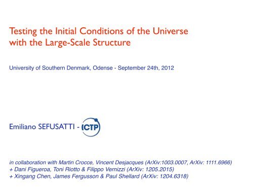
Testing <strong>the</strong> Initial Conditions of <strong>the</strong> Universe<br />
with <strong>the</strong> Large-Scale Structure<br />
University of Sou<strong>the</strong>rn Denmark, Odense - September 24th, 2012<br />
Emiliano SEFUSATTI - ICTP<br />
in collaboration with Martin Crocce, Vincent Desjacques (ArXiv:1003.0007, ArXiv: 1111.6966)<br />
+ Dani Figueroa, Toni Riotto & Filippo Vernizzi (ArXiv: 1205.2015)<br />
+ Xingang Chen, James Fergusson & Paul Shellard (ArXiv: 1204.6318)
Outline<br />
• Inflation, Primordial non-Gaussianity & <strong>the</strong> CMB<br />
• (Non-primordial) non-Gaussianity in <strong>the</strong> Large-Scale Structure<br />
• Primordial non-Gaussianity in <strong>the</strong> matter distribution<br />
• Primordial non-Gaussianity in <strong>the</strong> galaxy distribution
Part 1<br />
The “shapes” of Inflation & <strong>the</strong> CMB<br />
Text<br />
!"#$"%&'(%")* +, )-).)<br />
Polarization * +, )-).)<br />
!"#$"%&'(%")* +, )-)/...)<br />
012&%34&516)* +, )-)/...)
Primordial non-Gaussianity<br />
The Gaussianity of primordial fluctuations is one of <strong>the</strong> basic<br />
predictions of <strong>the</strong> simplest model of inflation<br />
confirmed (so far) at 0.1% level by CMB observations<br />
Therefore ...<br />
<strong>the</strong> possible detection of a large non-Gaussianity component in<br />
<strong>the</strong> intial conditions would, by itself, rule-out canonical,<br />
single-field, slow-roll inflation, providing a tool to<br />
discriminate between models of inflation
Non-Gaussian Initial Conditions<br />
Gaussian initial conditions:<br />
• <strong>the</strong>ir statistical properties are completely specified by <strong>the</strong> two-point<br />
correlation function or <strong>the</strong> power spectrum of <strong>the</strong> curvature<br />
perturbations:<br />
• All higher-order correlation functions are vanishing<br />
Bispectrum:<br />
Φ k1 Φ k2 = δ D ( k 1 + k 2 )P Φ (k 1 )<br />
Φ k1 Φ k2 Φ k3 = δ D ( k 1 + k 2 + k 3 ) B Φ (k 1 ,k 2 ,k 3 )=0<br />
Trispectrum:<br />
Φ k1 Φ k2 Φ k3 Φ k4 = δ D ( k 1 + ... + k 4 ) T Φ ( k 1 , k 2 , k 3 , k 4 )=0<br />
Non-Gaussian initial conditions are<br />
characterized by an infinite set of functions:<br />
B Φ (k 1 ,k 2 ,k 3 ) = 0<br />
T Φ ( k 1 , k 2 , k 3 , k 4 ) = 0<br />
, etc ...
Models of primordial non-Gaussianity<br />
Local non-Gaussianity:<br />
A quadratic correction to <strong>the</strong> initial curvature perturbations, Φ:<br />
Φ(x) =φ(x)+f NL φ 2 (x)<br />
leading to <strong>the</strong> initial, curvature bispectrum<br />
B Φ (k 1 ,k 2 ,k 3 )=2f NL P φ (k 1 )P φ (k 2 )+2perm.<br />
with specific properties:<br />
• large values for squeezed triangular configurations<br />
• well represents <strong>the</strong>oretical models where perturbations are<br />
generated outside <strong>the</strong> horizon: curvaton, multiple-field<br />
inflation, inhomogeneous preheating, ....<br />
Equilateral non-Gaussianity:<br />
k 1<br />
k 2<br />
<br />
<br />
B Φ (k 1 ,k 2 ,k 3 )=6f NL −P φ (k 1 )P φ (k 2 )+perm. − 2P 2/3<br />
φ (k 1)P 2/3<br />
φ (k 2)P 2/3<br />
φ (k 3)+...<br />
k 3<br />
• large values for equilateral triangular configurations<br />
• well approximates <strong>the</strong> bispectrum predicted by DBI inflation<br />
or higher derivative models<br />
Orthogonal non-Gaussianity ... and many more<br />
k 1 k 2<br />
k 3
The slang of non-Gaussianity<br />
Most inflationary models predict a scale-invariant curvature bispectrum<br />
B Φ (k, k, k) ∼ P 2 Φ(k) ∼ 1 k 6<br />
What distinguish <strong>the</strong>m is <strong>the</strong> shape<br />
“shape” = <strong>the</strong> dependence of <strong>the</strong> curvature bispectrum predicted<br />
by a given model of inflation on <strong>the</strong> shape of <strong>the</strong> triangular<br />
configuration k1, k2, k3<br />
B Φ (k 1 ,k 2 ,k 3 )=f NL<br />
1<br />
k 2 1 k2 2 k2 3<br />
F<br />
<br />
r 2 = k 2<br />
k 1<br />
,r 3 = k 3<br />
k 1
Models of primordial non-Gaussianity<br />
id est,<br />
Multiple fields<br />
courtesy of G. DʼAmico
The CMB Bispectrum<br />
The Bispectrum of <strong>the</strong> CMB is <strong>the</strong> most<br />
direct probe of <strong>the</strong> initial bispectrum<br />
B l1 l 2 l 3<br />
<br />
∼<br />
B Φ (k 1 ,k 2 ,k 3 )∆ l1 (k 1 )∆ l2 (k 2 )∆ l3 (k 3 )j l1 (k 1 r)j l2 (k 2 r)j l3 (k 3 r)<br />
CMB angular<br />
bispectrum<br />
curvature<br />
bispectrum<br />
transfer<br />
functions<br />
• The CMB provides a snapshot of density perturbations at early times<br />
• Power spectrum measurements (Clʼs) are matched by linear predictions (so far)<br />
• The CMB bispectrum is an optimal estimator for <strong>the</strong> fNL parameter
The CMB Bispectrum<br />
The Bispectrum of <strong>the</strong> CMB is <strong>the</strong> most<br />
direct probe of <strong>the</strong> initial bispectrum<br />
B l1 l 2 l 3<br />
<br />
∼<br />
B Φ (k 1 ,k 2 ,k 3 )∆ l1 (k 1 )∆ l2 (k 2 )∆ l3 (k 3 )j l1 (k 1 r)j l2 (k 2 r)j l3 (k 3 r)<br />
CMB angular<br />
bispectrum<br />
curvature<br />
bispectrum<br />
transfer<br />
functions<br />
• The CMB provides a snapshot of density perturbations at early times<br />
• Power spectrum measurements (Clʼs) are matched by linear predictions (so far)<br />
• The CMB bispectrum is an optimal estimator for <strong>the</strong> fNL parameter<br />
No evidence (yet)!<br />
(despite 2-sigma “hints” in<br />
previous data releases ...)<br />
WMAP 7 years:<br />
Local -10 < fNL < 74<br />
Equilateral -214 < fNL < 266<br />
Orthogonal -410 < fNL < 6<br />
@ 95% CL Komatsu et al. (2011)<br />
The CMB bispectrum is equally sensitive to any model of non-Gaussianity
The CMB Bispectrum<br />
The Bispectrum of <strong>the</strong> CMB is <strong>the</strong> most<br />
direct probe of <strong>the</strong> initial bispectrum<br />
B l1 l 2 l 3<br />
<br />
∼<br />
B Φ (k 1 ,k 2 ,k 3 )∆ l1 (k 1 )∆ l2 (k 2 )∆ l3 (k 3 )j l1 (k 1 r)j l2 (k 2 r)j l3 (k 3 r)<br />
CMB angular<br />
bispectrum<br />
curvature<br />
bispectrum<br />
transfer<br />
functions<br />
• The CMB provides a snapshot of density perturbations at early times<br />
• Power spectrum measurements (Clʼs) are matched by linear predictions (so far)<br />
• The CMB bispectrum is an optimal estimator for <strong>the</strong> fNL parameter<br />
No evidence (yet)!<br />
(despite 2-sigma “hints” in<br />
previous data releases ...)<br />
Planck will improve WMAP<br />
results by a factor of ~ 4<br />
ΔfNL<br />
local<br />
ΔfNL<br />
equilateral<br />
WMAP 21 140<br />
Planck ~ 5 ~ 30<br />
The CMB bispectrum is equally sensitive to any model of non-Gaussianity
Part 1I<br />
(Non-primordial) non-Gaussianity in <strong>the</strong> Large-Scale Structure
Non-Gaussianity in <strong>the</strong> Large-Scale Structure<br />
250<br />
250<br />
200<br />
200<br />
150<br />
150<br />
100<br />
100<br />
50<br />
50<br />
0<br />
0<br />
0 50 100 150 200 250<br />
Mock galaxy distribution<br />
0 50 100 150 200 250<br />
Rayleigh-Lévy flight<br />
ES & Scoccimarro (2005)
Non-Gaussianity in <strong>the</strong> Large-Scale Structure<br />
250<br />
250<br />
200<br />
150<br />
100<br />
200<br />
150<br />
100<br />
Cosmological parameters and<br />
constraints on <strong>the</strong> initial<br />
conditions are typically obtained<br />
<strong>from</strong> power spectrum<br />
measurements<br />
50<br />
50<br />
0<br />
0<br />
0 50 100 150 200 250<br />
0 50 100 150 200 250<br />
-Gaussianity in <strong>the</strong> Large-Scale Structure<br />
<strong>the</strong> power spectrum<br />
cannot distinguish <strong>the</strong><br />
two distributions!<br />
edshift surveys, information on cosmological parameters and <strong>the</strong> initial<br />
ditions is typically obtained <strong>from</strong> measurements of <strong>the</strong> power spectrum<br />
δ k δ k ≡δ D ( k + k )P(k) where δ k FT ↔ δ(x) ≡<br />
ρ(x) − ¯ρ<br />
¯ρ<br />
250<br />
ES & Scoccimarro (2005)
Non-Gaussianity in <strong>the</strong> Large-Scale Structure<br />
250<br />
250<br />
200<br />
150<br />
100<br />
200<br />
150<br />
100<br />
Cosmological parameters and<br />
constraints on <strong>the</strong> initial<br />
conditions are typically obtained<br />
<strong>from</strong> power spectrum<br />
measurements<br />
-Gaussianity in <strong>the</strong> Large-Scale Structure<br />
50<br />
50<br />
t <strong>the</strong>ir non-Gaussian properties, quantifiedby<strong>the</strong>irhigher-ordercorrelation<br />
0<br />
ctions are clearly different:<br />
0 50 100 150 200 250<br />
0<br />
0 50 100 150 200 250<br />
Bispectrum:<br />
δ k1 δ k2 δ k3 ≡δ D ( k 123 )B(k 1 , k 2 , k 3 )<br />
cture<br />
k3<br />
k1<br />
✁<br />
❍ ❍<br />
✁☛ ✟ ✟✟✯ k2<br />
dby<strong>the</strong>irhigher-ordercorrelation<br />
Trispectrum:<br />
rispectrum:<br />
250<br />
δ k1 δ k2 δ k3 δ k4 c ≡ δ D ( k 1234 )T ( k 1 , k 2 , k 3 , k 4 )<br />
200<br />
✁<br />
✁☛<br />
150<br />
k4<br />
❍ ❍<br />
✲ ✻<br />
k1<br />
k2<br />
k3<br />
trispectrum:<br />
δ k1 δ k2 δ k3 δ k4 c ≡ δ D ( k 1234 )T ( k 1 , k 2 , k 3 , k 4 )<br />
⇒<br />
k4<br />
k1<br />
✁<br />
❍ ❍<br />
✁☛ ✲ ✻ k3<br />
k2<br />
<strong>the</strong> power spectrum<br />
cannot distinguish <strong>the</strong><br />
two distributions!<br />
but <strong>the</strong>ir non-Gaussian<br />
properties are very<br />
different!<br />
100<br />
ES & Scoccimarro (2005)<br />
50
Non-Gaussianity <strong>from</strong> Gravitational Instability<br />
A fundamental quantity: <strong>the</strong> matter overdensity<br />
δ(x) ≡<br />
ρ(x) − ¯ρ<br />
¯ρ<br />
≥−1<br />
At early times (z ~ 1000)fluctuations<br />
are small (σδ≪1):<br />
⟨δδ⟩≠0,<br />
⟨δδδ⟩≃0<br />
⟨δδδδ⟩≃0<br />
At late times fluctuations grow, σδ >1<br />
Non-Gaussianity is induced by<br />
gravitational evolution<br />
⟨δδ⟩≠0,<br />
⟨δδδ⟩≠0<br />
⟨δδδδ⟩≠0
Non-Gaussianity <strong>from</strong> Gravitational Instability<br />
At large scales fluctuations are small, σδ≪1, even at low redshift<br />
we can study <strong>the</strong>ir evolution in terms of Perturbation Theory<br />
Equations of motion for<br />
matter density and velocity:<br />
δ, v<br />
• Continuity eq.<br />
• Euler eq.<br />
• Poisson eq.<br />
∂δ<br />
+ ∇ · [(1 + δ)v] =0<br />
∂τ<br />
∂v<br />
∂τ + Hv +(v · ∇)v = −∇φ<br />
<br />
∇ 2 φ = 3 2 H2 Ω m δ
Non-Gaussianity <strong>from</strong> Gravitational Instability<br />
At large scales fluctuations are small, σδ≪1, even at low redshift<br />
we can study <strong>the</strong>ir evolution in terms of Perturbation Theory<br />
Equations of motion for<br />
matter density and velocity:<br />
δ, v<br />
• Continuity eq.<br />
• Euler eq.<br />
• Poisson eq.<br />
∂δ<br />
+ ∇ · [(1 + δ)v] =0<br />
∂τ<br />
∂v<br />
∂τ + Hv +(v · ∇)v = −∇φ<br />
<br />
∇ 2 φ = 3 2 H2 Ω m δ<br />
Perturbative solution for <strong>the</strong><br />
matter density, in Fourier space<br />
δ k = δ (1)<br />
k<br />
+ δ (2)<br />
k<br />
+ ...<br />
Linear solution<br />
δ (2)<br />
k<br />
=<br />
<br />
d 3 qF 2 ( k − q, q) δ (1)<br />
<br />
δ (1)<br />
k−q q<br />
Quadratic nonlinear correction
Non-Gaussianity <strong>from</strong> Gravitational Instability<br />
At large scales fluctuations are small, σδ≪1, even at low redshift<br />
we can study <strong>the</strong>ir evolution in terms of Perturbation Theory<br />
Equations of motion for<br />
matter density and velocity:<br />
δ, v<br />
Perturbative solution for <strong>the</strong><br />
matter density, in Fourier space<br />
• Continuity eq.<br />
• Euler eq.<br />
• Poisson eq.<br />
δ k = δ (1)<br />
k<br />
+ δ (2)<br />
k<br />
+ ...<br />
Linear solution<br />
∂δ<br />
+ ∇ · [(1 + δ)v] =0<br />
∂τ<br />
∂v<br />
∂τ + Hv +(v · ∇)v = −∇φ<br />
<br />
∇ 2 φ = 3 2 H2 Ω m δ<br />
δ (2)<br />
k<br />
=<br />
Initial conditions δ (1)<br />
k1<br />
δ (1)<br />
k2<br />
= δ D ( k 1 + k 2 )P 0 (k 1 )<br />
B0 and T0 vanish for<br />
Gaussian initial conditions!<br />
<br />
d 3 qF 2 ( k − q, q) δ (1)<br />
<br />
δ (1)<br />
k−q q<br />
Quadratic nonlinear correction<br />
δ (1)<br />
k1<br />
δ (1)<br />
k2<br />
δ (1)<br />
k3<br />
= δ D ( k 1 + k 2 + k 3 ) B 0 (k 1 ,k 2 ,k 3 )<br />
δ (1)<br />
k1<br />
δ (1)<br />
k2<br />
δ (1)<br />
k3<br />
δ (1)<br />
k4<br />
= δ D ( k 1 + ... + k 4 ) T 0 ( k 1 , k 2 , k 3 , k 4 )
Non-Gaussianity <strong>from</strong> Gravitational Instability<br />
At large scales fluctuations are small, σδ≪1, even at low redshift<br />
we can study <strong>the</strong>ir evolution in terms of Perturbation Theory<br />
Equations of motion for<br />
matter density and velocity:<br />
δ, v<br />
Perturbative solution for <strong>the</strong><br />
matter density, in Fourier space<br />
δ k = δ (1)<br />
k<br />
+ δ (2)<br />
k<br />
+ ...<br />
Linear solution<br />
δ (2)<br />
k<br />
=<br />
Initial conditions δ (1)<br />
k1<br />
δ (1)<br />
k2<br />
= δ D ( k 1 + k 2 )P 0 (k 1 )<br />
B0 and T0 vanish for<br />
Gaussian initial conditions!<br />
• Continuity eq.<br />
• Euler eq.<br />
• Poisson eq.<br />
∂δ<br />
+ ∇ · [(1 + δ)v] =0<br />
∂τ<br />
∂v<br />
∂τ + Hv +(v · ∇)v = −∇φ<br />
<br />
∇ 2 φ = 3 2 H2 Ω m δ<br />
<br />
d 3 qF 2 ( k − q, q) δ (1)<br />
<br />
δ (1)<br />
k−q q<br />
Quadratic nonlinear correction<br />
δ (1)<br />
k1<br />
δ (1)<br />
k2<br />
δ (1)<br />
k3<br />
= δ D ( k 1 + k 2 + k 3 ) B 0 (k 1 ,k 2 ,k 3 )<br />
δ (1)<br />
k1<br />
δ (1)<br />
k2<br />
δ (1)<br />
k3<br />
δ (1)<br />
k4<br />
= δ D ( k 1 + ... + k 4 ) T 0 ( k 1 , k 2 , k 3 , k 4 )<br />
Perturbative solution for <strong>the</strong><br />
matter 3-point function<br />
δδδ = δ (1) δ (1) δ (1) + δ (1) δ (1) δ (2) + ...<br />
loop corrections<br />
= B0 = 0 for Gaussian<br />
initial conditions<br />
non-zero bispectrum<br />
induced by gravity!
The Matter Bispectrum induced by Gravity<br />
ateral configurations of <strong>the</strong> matter bispectrum<br />
B G = BG<br />
tree [P 0 ]+B loop<br />
G [P 0]<br />
and <strong>the</strong> linear and 1-loop predictions in PT a<br />
BG<br />
tree<br />
(k 1 ,k 2 ,k 3 )=2F 2 ( k 1 , k 2 ) P 0 (k 1 ) P 0 (k 2 )+2perm.<br />
The bispectrum induced by gravity has a well defined<br />
dependence on scale and on <strong>the</strong> shape<br />
Bk, k, k<br />
110 4<br />
5000<br />
1000<br />
500<br />
matter bispectrum<br />
equilateral configurations<br />
f NL 0<br />
z 0.5<br />
1-loop<br />
Bk, k, k<br />
The equilateral configurations<br />
of <strong>the</strong> matter bispectrum:<br />
B(k, k, k) vs. k<br />
Numerical 1000 simulations and PT<br />
predictions<br />
100<br />
100<br />
50<br />
Tree-level<br />
10<br />
10 4 k h Mpc 1<br />
E.S., M. Crocce, & V. Desjacques (2010)<br />
F. Bernardeau, M. Crocce, E.S. (2010)<br />
0.01 0.02 0.05 0.10 0.20<br />
k h Mpc 1 <br />
0.01 0.02 0.05
The Matter Bispectrum induced by Gravity<br />
The bispectrum represents <strong>the</strong> probability for three particles<br />
(or galaxies) to form a triangle of a given size and shape<br />
Plot of <strong>the</strong> reduced bispectrum Q(k1, k2, k3)<br />
with fixed k1 and k2 as a function of <strong>the</strong><br />
angle between <strong>the</strong> two wavenumbers<br />
2.5<br />
Q(k 1 ,k 2 ,k 3 )=<br />
B(k 1 ,k 2 ,k 3 )<br />
P (k 1 )P (k 2 )+P (k 1 )P (k 3 )+P (k 2 )P (k 3 )<br />
Qk1,k2,Θ<br />
2.0<br />
1.5<br />
Nbody<br />
treelevel<br />
1loop<br />
k 1 0.094 h 1 Mpc<br />
k 2 2k 1<br />
1.0<br />
0.5<br />
matter bispectrum<br />
f NL 0, z 0.5<br />
0.0 0.2 0.4 0.6 0.8 1.0<br />
Θ<br />
k 1<br />
k 2<br />
k 3 Θ<br />
ΘΠ
Non-Gaussianity <strong>from</strong> Galaxy Bias (more problems?)<br />
Additional non-Gaussianity in <strong>the</strong> galaxy distribution<br />
is induced by nonlinear galaxy bias<br />
The relation between <strong>the</strong><br />
observed galaxy<br />
overdensity and <strong>the</strong> matter<br />
density is nonlinear<br />
δ g (x) ≡ n g(x) − ¯n g<br />
¯n g<br />
= f [δ(x)]<br />
local bias<br />
At large scales, we expand it in<br />
a Taylor series<br />
δ g (x) =b 1 δ(x)+ 1 2 b 2 δ 2 (x)+...<br />
Linear bias<br />
Quadratic bias correction<br />
Perturbative solution for <strong>the</strong><br />
galaxy 3-point function<br />
δ g δ g δ g = b 3 1 δδδ + b 2 1 b 2 δδδ 2 + ...<br />
matter bispectrum<br />
bispectrum induced<br />
by nonlinear bias<br />
B g (k 1 ,k 2 ,k 3 )=b 3 1 B(k 1 ,k 2 ,k 3 )+b 2 1 b 2 P (k 1 ) P (k 2 )+2perm. + ...<br />
The component induced by bias has a different<br />
dependence on <strong>the</strong> shape of <strong>the</strong> triangle
From <strong>the</strong> CMB to <strong>the</strong> Large-Scale Structure<br />
The CMB provides a snapshot of <strong>the</strong> Universe at<br />
very high redshift and its power spectrum<br />
(<strong>the</strong> Cl’s) is matched by linear predictions<br />
The observable Universe to <strong>the</strong><br />
CMB last scattering surface<br />
The Large-Scale Structure is <strong>the</strong> result<br />
of a highly nonlinear evolution, with<br />
different sources of non-Gaussianity<br />
How can we distinguish and detect<br />
<strong>the</strong> primordial component?<br />
Why bo<strong>the</strong>r at all?!<br />
The Sloan Digital Sky Survey<br />
(white dots are galaxies)
From <strong>the</strong> CMB to <strong>the</strong> Large-Scale Structure<br />
The CMB provides a snapshot of <strong>the</strong> Universe at<br />
very high redshift and its power spectrum<br />
(<strong>the</strong> Cl’s) is matched by linear predictions<br />
The observable Universe to <strong>the</strong><br />
CMB last scattering surface<br />
The Large-Scale Structure is <strong>the</strong> result<br />
of a highly nonlinear evolution, with<br />
different sources of non-Gaussianity<br />
How can we distinguish and detect<br />
<strong>the</strong> primordial component?<br />
Why bo<strong>the</strong>r at all?!<br />
Two reasons:<br />
The Sloan Digital Sky Survey<br />
(white dots are galaxies)<br />
1. The CMB is 2D field, <strong>the</strong> LSS is 3D<br />
2. Galaxy bias reserved a surprise for us ...
Part III<br />
Matter<br />
400 particles. Since we are interested mainly in <strong>the</strong> masses<br />
and positions of cluster-sized halos, and not <strong>the</strong>ir internal<br />
structure, we have not used high force resolution: we<br />
employ a Plummer softening length l of 0.2 times <strong>the</strong><br />
mean interparticle spacing. We have checked that using<br />
higher force resolution (l half as large) does not appreciably<br />
change <strong>the</strong> mass function. All simulations were performed<br />
at <strong>the</strong> Sunnyvale cluster at CITA; depending upon<br />
We c<br />
z ¼ 1, 0<br />
[66], w<br />
tions, th<br />
extensiv<br />
are plot<br />
fNL = - 5000<br />
fNL = - 500<br />
fNL = 0<br />
Havin<br />
like to c<br />
used fo<br />
above,<br />
Gaussia<br />
Schecht<br />
function<br />
order o<br />
interest<br />
to <strong>the</strong><br />
adopted<br />
fNL = + 500<br />
( )<br />
fNL = + 5000<br />
Dalal et al. (2008)<br />
FIG. 1 (color online). Slice through simulation outputs at z ¼<br />
0 generated with <strong>the</strong> same Fourier phases but with f ¼
Matter Power Spectrum<br />
In Perturbation Theory ...<br />
P = P 0 + P loop<br />
G<br />
[P 0]+P loop<br />
NG [P 0,B 0 ]<br />
matter power spectrum<br />
Linear power<br />
spectrum<br />
Gravity-induced<br />
contributions<br />
(depending on P0 alone)<br />
Additional gravity-induced contributions<br />
present only for NG initial conditions (B0)
Matter Power Spectrum<br />
In Perturbation Theory ...<br />
P = P 0 + P loop<br />
G<br />
[P 0]+P loop<br />
NG [P 0,B 0 ]<br />
matter power spectrum<br />
Linear power<br />
spectrum<br />
Gravity-induced<br />
contributions<br />
(depending on P0 alone)<br />
Additional gravity-induced contributions<br />
present only for NG initial conditions (B0)<br />
Few percent effect at small scales<br />
for allowed values of fNL<br />
Ratio of <strong>the</strong> non-Gaussian<br />
to <strong>the</strong> Gaussian power<br />
spectrum for fNL = ±100<br />
(local) at z =1<br />
Smith, Desjacques & Marian (2010)
Matter Power Spectrum<br />
In Perturbation Theory ...<br />
P = P 0 + P loop<br />
G<br />
[P 0]+P loop<br />
NG [P 0,B 0 ]<br />
Linear power<br />
spectrum<br />
Gravity-induced<br />
contributions<br />
(depending on P0 alone)<br />
Additional gravity-induced contributions<br />
present only for NG initial conditions (B0)<br />
Few percent effect at small scales<br />
. for Fedeli allowed and L. Moscardini values of fNL<br />
Weak Lensing<br />
Ratio of <strong>the</strong> non-Gaussian<br />
to <strong>the</strong> Gaussian power<br />
spectrum for fNL = ±100<br />
(local) at z =1<br />
Smith, Desjacques & Marian (2010)<br />
Fedeli & Moscardini (2010)<br />
Giannantonio et al. (2011)<br />
From EUCLID we expect:<br />
ΔfNL ~ 20 (local)<br />
ΔfNL ~ 3 (orthogonal)<br />
ΔfNL ~ 10 (equilateral)<br />
(with Planck priors on<br />
cosmology)
Matter Power Spectrum & Bispectrum<br />
In Perturbation Theory ...<br />
P = P 0 + P loop<br />
G<br />
[P 0]+P loop<br />
NG [P 0,B 0 ]<br />
matter power spectrum<br />
Linear power<br />
spectrum<br />
Gravity-induced<br />
contributions<br />
(depending on P0 alone)<br />
Additional gravity-induced contributions<br />
present only for NG initial conditions (B0)<br />
B = B 0 + B tree<br />
G<br />
[P 0 ]+B loop<br />
G<br />
[P 0]+B loop<br />
NG [P 0,B 0 ]<br />
& bispectrum<br />
Primordial<br />
component
The matter bispectrum and PNG: large scales<br />
At large scales I can approximate <strong>the</strong> matter bispectrum with <strong>the</strong> tree-level expression on PT:<br />
B(k 1 ,k 2 ,k 3 ) B 0 + B tree<br />
G [P 0 ]<br />
Primordial<br />
component<br />
Gravity-induced<br />
component<br />
Bk,k,k<br />
5000<br />
2000<br />
1000<br />
500<br />
200<br />
Gravity<br />
Initial, f NL 100<br />
Gravity Initial<br />
0.01 0.02 0.05 0.1<br />
k h Mpc 1 <br />
Equilateral configurations<br />
of <strong>the</strong> matter bispectrum<br />
B 0 (k, k, k) k→0<br />
(k, k, k) ∼<br />
B tree<br />
G<br />
f NL<br />
D(z)k 2<br />
The primordial component has a<br />
different dependence on scale<br />
than <strong>the</strong> gravity-induced one!<br />
It is relevant at large scales<br />
and early times<br />
This is true for almost all models (local,<br />
equilateral, orthogonal ...)
The matter bispectrum and PNG: large scales<br />
At large scales I can approximate <strong>the</strong> matter bispectrum with <strong>the</strong> tree-level expression on PT:<br />
B(k 1 ,k 2 ,k 3 ) B 0 + B tree<br />
G [P 0 ]<br />
Primordial<br />
component<br />
Gravity-induced<br />
component<br />
1.4<br />
1.2<br />
k 1 =0.01 h Mpc −1 , k 2 =1.5 k 1<br />
Reduced bispectrum as a function of<br />
<strong>the</strong> angle between two wavenumbers<br />
Qk 1 ,k 2 ,Θ<br />
1.0<br />
0.8<br />
0.6<br />
0.4<br />
0.2<br />
Gravity<br />
Initial, f NL 100<br />
Gravity Initial<br />
Primordial component for<br />
local non-Gaussianity:<br />
large contribution in <strong>the</strong><br />
squeezed limit!<br />
The primordial component has<br />
a different dependence on <strong>the</strong><br />
shape of <strong>the</strong> triangular<br />
configurations<br />
0.0 0.2 0.4 0.6 0.8 1.0<br />
ΘΠ<br />
and it is specific to <strong>the</strong> non-Gaussian<br />
model (local, equilateral, orthogonal ...)
The matter bispectrum and PNG: large scales<br />
Qk 1 ,k 2 ,Θ<br />
2.5<br />
2.0<br />
1.5<br />
1.0<br />
Local NG, 10 f NL 74<br />
Current CMB constraints for different<br />
models of non-Gaussianity as uncertainties<br />
on <strong>the</strong> generic configurations of <strong>the</strong> matter<br />
bispectrum, B B 0 + BG tree [P 0 ]<br />
0.5<br />
The matter bispectrum can distinguish<br />
different non-Gaussian models<br />
0.0 0.2 0.4 0.6 0.8 1.0<br />
ΘΠ<br />
2.5<br />
Equilateral NG, 214 f NL 266<br />
2.5<br />
Orthogonal NG, 410 f NL 6<br />
2.0<br />
2.0<br />
Qk 1 ,k 2 ,Θ<br />
1.5<br />
1.0<br />
Qk 1 ,k 2 ,Θ<br />
1.5<br />
1.0<br />
0.5<br />
0.5<br />
0.0 0.2 0.4 0.6 0.8 1.0<br />
ΘΠ<br />
0.0 0.2 0.4 0.6 0.8 1.0<br />
ΘΠ
The matter bispectrum and PNG: large scales<br />
In Perturbation Theory ...<br />
P = P 0 + P loop<br />
G<br />
[P 0]+P loop<br />
NG [P 0,B 0 ]<br />
matter power spectrum<br />
Linear power<br />
spectrum<br />
Gravity-induced<br />
contributions<br />
(depending on P0 alone)<br />
Additional gravity-induced contributions<br />
present only for NG initial conditions (B0)<br />
B = B 0 + B tree<br />
G<br />
[P 0 ]+B loop<br />
G<br />
[P 0]+B loop<br />
NG [P 0,B 0 ]<br />
& bispectrum<br />
Primordial<br />
component<br />
If B0 was <strong>the</strong> only effect of NG initial conditions on <strong>the</strong> LSS<br />
<strong>the</strong>n future, large volume surveys (~100 Gpc 3 ) could<br />
provide:<br />
ΔfNL local < 5 and ΔfNL eq < 10<br />
Scoccimarro, ES & Zaldarriaga (2004), ES & Komatsu (2007)
The matter bispectrum and PNG: small scales<br />
In Perturbation Theory ...<br />
P = P 0 + P loop<br />
G<br />
[P 0]+P loop<br />
NG [P 0,B 0 ]<br />
matter power spectrum<br />
Linear power<br />
spectrum<br />
Gravity-induced<br />
contributions<br />
(depending on P0 alone)<br />
Additional gravity-induced contributions<br />
present only for NG initial conditions (B0)<br />
B = B 0 + B tree<br />
G<br />
[P 0 ]+B loop<br />
G<br />
[P 0]+B loop<br />
NG [P 0,B 0 ]<br />
& bispectrum<br />
Primordial<br />
component<br />
Nonlinear corrections are also<br />
affected by <strong>the</strong> initial conditions!
B G B G, tree, nw<br />
BNG<br />
BNG BG<br />
BG<br />
1.6<br />
1.4<br />
The matter bispectrum and PNG:<br />
1.4<br />
small scales<br />
1.4<br />
1.2<br />
1.2<br />
B = 1.3 B 0 + BG<br />
tree<br />
1.0<br />
BNG BG<br />
0.8 1.2 Primordial Gravity-induced Additional gravity-induced 0.8 1.2 contributions<br />
component contributions present for NG initial conditions (B0)<br />
0.6<br />
0.05 0.10 0.15 0.20 0.25 0.30<br />
1.1<br />
1.1<br />
0.05 0.10 0.15 0.20 0.25 0.30<br />
k h Mpc 1 <br />
k h Mpc 1 <br />
Squeezed 1.0 configurations B(Δk, k, k)<br />
as a function of k with Δk = 0.01 h/Mpc<br />
1.4<br />
1000<br />
1.3500<br />
1.2200<br />
100<br />
1.1<br />
50<br />
treelevel<br />
oneloop<br />
SC01<br />
ES (2009)<br />
ES, Crocce & Desjacques (2010)<br />
1.0<br />
5000<br />
Ratio B f NL 100 B f NL 0<br />
[P 0 ]+B loop<br />
G<br />
1.0<br />
0.05Squeezed 0.10 0.15configurations 0.20 0.25 0.30 B(∆k, k, k) vs. 0.05 k, 0.10 non-Gaussian ES 0.15 (2009) 0.20 0.25 initial 0.30c<br />
k h Mpc 1 <br />
Ratio Difference B f NL B f100 NL 100 B f NL B f NL 00<br />
z 0z 1<br />
0.010.05 0.02 0.10 0.15 0.05 0.200.10 0.25 0.20.30<br />
k hk Mpc h Mpc 1 <br />
1 <br />
Nbody<br />
treelevel<br />
oneloop<br />
[P 0]+B loop<br />
B G B G, tree, nw<br />
z 1<br />
1.0<br />
1.3<br />
NG [P 0,B 0 ]<br />
BNG BG<br />
BNG BG<br />
200<br />
1.3<br />
BNG BG<br />
1.4<br />
1.2<br />
1.1<br />
1.0<br />
100<br />
50<br />
20<br />
10<br />
Ratio B f NL 100 B f NL 0<br />
k h Mpc 1 <br />
z 2<br />
ES, Crocce & Desjacques (2010)<br />
Ratio Difference B f NL B f100 NL 100 B f NL B f NL<br />
00<br />
z z1<br />
2<br />
0.010.05 0.02 0.10 0.15 0.05 0.200.10 0.25 0.200.30<br />
k hk Mpc h Mpc 1 <br />
1
0.8<br />
0.6<br />
0.01 0.1 1 10<br />
k h Mpc 1 <br />
The matter bispectrum and PNG: even smaller scales<br />
N<br />
Beyond PT: The Halo Model<br />
1000<br />
Difference B f NL 100 B f NL 0<br />
BNG BG<br />
100<br />
10<br />
There is a significant effect of NG<br />
initial conditions of about 5-15% on all<br />
triangles, at small scales and at late<br />
times for fNL = 100<br />
Weak lensing?<br />
NbodyHM<br />
1<br />
1.40.01 0.1 Nbody 1 HM<br />
1.2<br />
1.0<br />
k h Mpc 1 <br />
10<br />
0.8<br />
0.6<br />
0.01 0.1 1 10<br />
k h Mpc 1 <br />
1.3<br />
Ratio B f NL 100 B f NL 0<br />
BNG BG<br />
1.2<br />
1.1<br />
Figueroa, ES, Riotto & Vernizzi (2012)<br />
Squeezed configurations B(Δk, k, k)<br />
as a function of k with Δk = 0.01 h/Mpc<br />
1.0<br />
0.01 0.1 1 10<br />
k h Mpc 1
Part IV<br />
Galaxies<br />
IMPRINTS OF PRIMORDIAL NON-GAUSSIANITIES ON ...<br />
fNL = - 5000<br />
fNL = - 500<br />
fNL = 0<br />
fNL = + 500<br />
fNL = + 5000<br />
Dalal et al. (2008)<br />
FIG. 7 (color online). Cross-power spectra for various f NL .<br />
The upper panel displays P h ðkÞ, measured in our simulations at<br />
z ¼ 1 for halos of mass 1:6 10 13 M
Galaxy bias and <strong>the</strong> galaxy power spectrum<br />
Dalal et al. (2008):<br />
The bias of galaxies receives a significant scale-dependent<br />
correction for NG initial conditions of <strong>the</strong> local type<br />
P g (k) =[b 1 + ∆b 1 (f NL ,k)] 2 P (k)<br />
“Gaussian” Scale-dependent correction<br />
IMPRINTS OF biasPRIMORDIAL due NON-GAUSSIANITIES to local non-GaussianityON ...<br />
Large effect on large scales!<br />
Dalal et al. (2008)<br />
PHYSICAL REVIEW<br />
using <strong>the</strong> halo auto spectra to compute<br />
results as <strong>the</strong> cross spectra; i.e. we<br />
stochasticity. Examples of <strong>the</strong> variou<br />
resulting bias factors are plotted in F<br />
As can be seen, we numerically co<br />
∆b predicted 1,NG (fscale NL ,k) dependence. ∼<br />
f NLBecau<br />
statistics of rare objects, D(z) <strong>the</strong> errors k 2 on<br />
simulations plotted in Fig. 8 are lar<br />
tempt to improve <strong>the</strong> statistics on <strong>the</strong><br />
bining <strong>the</strong> bias measurements <strong>from</strong><br />
Figure 8 plots <strong>the</strong> average ratio betwe<br />
in our simulations and our analytic<br />
using c ¼ 1:686 as predicted <strong>from</strong> t<br />
model [78]. In computing <strong>the</strong> average<br />
we used a uniform weighting across<br />
Measurements of <strong>the</strong> power spectrum of<br />
dark matter halos in N-body simulation<br />
with local NG initial conditions
Galaxy bias and <strong>the</strong> galaxy power spectrum<br />
Dalal et al. (2008):<br />
The bias of galaxies receives a significant scale-dependent<br />
correction for NG initial conditions of <strong>the</strong> local type<br />
P g (k) =[b 1 + ∆b 1 (f NL ,k)] 2 P (k)<br />
“Gaussian”<br />
bias<br />
Scale-dependent correction<br />
due to local non-Gaussianity<br />
QSOs+LRGs: -31 < fNL < 70 (95% CL)<br />
[Slosar et al. (2008)]<br />
AGNs+QSOs+LRGs: 8 < fNL < 88 (95% CL)<br />
[Xia et al. (2011)]<br />
Limits <strong>from</strong> LSS are<br />
already competitive<br />
with <strong>the</strong> CMB!<br />
(at least for <strong>the</strong> local model ...)<br />
high-redshift sources: quasars & AGNs<br />
CMB limits (95% CL): -10 < fNL < 74<br />
[Komatsu et al. (2009)]<br />
From EUCLID we expect:<br />
ΔfNL ~ 5<br />
<strong>from</strong> <strong>the</strong> 3D power spectrum alone<br />
[e.g. Giannantonio et al. (2011)]
shear<br />
by<br />
→<br />
n-<br />
ad<br />
we<br />
0).<br />
er-<br />
L)<br />
ng<br />
nd<br />
nt<br />
llias<br />
=<br />
et<br />
ses<br />
by<br />
w-<br />
Galaxy bias and <strong>the</strong> galaxy power spectrum<br />
Dalal et al. (2008):<br />
The bias of galaxies receives a significant scale-dependent<br />
correction for NG initial conditions of <strong>the</strong> local type<br />
FIG. 4: The scale-dependent part of bias b − b ∞ divided by<br />
b ∞ − 1, for f NL =100andz =0. Thescale-independent<br />
part of bias, b ∞ =1.5 and3forsolidanddottedcurves.The<br />
dashed line is Dalal et al.’s derivation [1].<br />
P g (k) =[b 1 + ∆b 1 (f NL ,k)] 2 P (k)<br />
“Gaussian”<br />
bias<br />
Afshordi & Tolley (2008)<br />
Scale-dependent correction<br />
due to local non-Gaussianity<br />
FIG. 5: This figure illustrates <strong>the</strong> contrast between <strong>the</strong> gaus-<br />
Introduction<br />
PNG and <strong>the</strong> Matter Bispectrum<br />
PNG and <strong>the</strong> Galaxy Bispectrum<br />
Future Perspectives<br />
A local model for primordial non-Gau<br />
Non-Gaussian Local non-Gaussianity<br />
correction to <strong>the</strong> curvatur<br />
introduces a correlation between h<br />
large-scale Φ(x) fluctuations =φ(x)+f and NL<br />
loc.<br />
<strong>the</strong> φ 2 (x) −<br />
small-scales responsible for <strong>the</strong><br />
[Salopek & Bond (19<br />
formation (collapse) of dark matter<br />
halos (and <strong>the</strong>refore, galaxies)<br />
⇒ B Φ (k 1 , k 2 , k 3 )=2fNL loc. [P φ (k 1 )P<br />
k 1<br />
k 2<br />
k 3<br />
Large val<br />
Represen<br />
are gener<br />
Curvato<br />
Multipl<br />
Inhomo
What about o<strong>the</strong>r models?<br />
approach [40]<br />
∆b I = b NG<br />
1 − b G 1 = − ∂ ln RNG (M)<br />
, (6.5)<br />
∂δ c<br />
The scale-dependence of bias can be different<br />
for o<strong>the</strong>r models, or not be <strong>the</strong>re at all ...<br />
R NG (M) being <strong>the</strong> ratio of <strong>the</strong> non-Gaussian to <strong>the</strong> Gaussian mass function. Here,<br />
ver, we treat ∆b I as a free parameter and compare it later on with <strong>the</strong> prediction<br />
ed <strong>from</strong> <strong>the</strong> mass functions. We choose q as <strong>the</strong> second free parameter. All o<strong>the</strong>r 1<br />
tities in Eq. (6.4) are we derive <strong>from</strong> <strong>the</strong> <strong>the</strong>ory and are kept fixed.<br />
In Fig. 8, we show as an example <strong>the</strong> effect of local non-Gaussianity on <strong>the</strong> halo bias<br />
alos of mass 1.2 − 2.4 × 10 14 M ⊙ /h at z = 0. Note that we plot ∆b(k)+0.1. As ∆b I is<br />
tive, this addition of 0.1 is needed to still make use of <strong>the</strong> logarithmic scale.<br />
The different line types visualize <strong>the</strong> effect of <strong>the</strong> different terms in Eq. (6.4). The 0.1<br />
s lines show <strong>the</strong> best fit to <strong>the</strong> data (using all modes up to k max =0.1Mpc/h) and<br />
des all terms given above. The short-dashed lines neglects ∆b I appearing inside <strong>the</strong><br />
re brackets in Eq. (6.4). The inclusion of this term makes <strong>the</strong> non-Gaussian bias nonr<br />
in f NL [55], since ∆b I depends on f NL . The dot-dashed line neglects ∆b I completely.<br />
scale-dependent bias shift becomes important on smaller scales (k >0.02), for which<br />
cale-dependent part becomes small.<br />
!b + 0.1<br />
10<br />
1<br />
0.1<br />
1<br />
k<br />
Orthogonal orthogonal NG<br />
Gaussian bias. This has <strong>the</strong> advantage that by doing this we do not need to include β(k<br />
<strong>the</strong> modelling of ∆b(k) (seeEq.(2.1) and Eq. (2.4)).<br />
!b + 0.1<br />
0.4<br />
f NL = -1000<br />
1.2x10 14 < M<br />
f NL = -250<br />
halo < 2.4x10 14<br />
3x10 13 < M halo < 6x10<br />
Figure 8. Local non-Gaussian bias of halos with mass 1.2 × 10 14 Mpc/h < 13<br />
M < 2.4 × 10 14 M<br />
at z = 0. The difference of <strong>the</strong> bias measured <strong>from</strong> <strong>the</strong> non-Gaussian simulations and Gau<br />
simulations is depicted 0.2 by <strong>the</strong> data points (for computation of <strong>the</strong> errorbars, see App. B). The<br />
lines show <strong>the</strong> best fit using <strong>the</strong> model given in Eq. 6.4. The dot-dashed lines show <strong>the</strong> m<br />
predictions when <strong>the</strong> scale-independent bias shift, ∆b I , is neglected. The short-dashed lines ne<br />
<strong>the</strong> term which is non-linear 0 in f NL (see text for details). Thick lines and red symbols correspon<br />
f NL = 250, while thin lines and blue symbols show <strong>the</strong> results for f NL = 60. Note that we act<br />
show ∆b +0.1 to allow for a logarithmic scale.<br />
!b<br />
10<br />
0.01<br />
0.003 0.01 0.1<br />
-0.2<br />
-0.4<br />
1<br />
k 2<br />
local<br />
Local NG<br />
k [h/Mpc]<br />
f NL = 250<br />
f NL = 60<br />
As <strong>the</strong> non-Gaussian and <strong>the</strong> Gaussian simulation share <strong>the</strong> same realization of<br />
initial Gaussian field, ∆b(k) is almost free of sample variance and, in addition, has sm<br />
shot noise than b NG (k) and b G (k) individually. We estimate <strong>the</strong> error on ∆b(k) directly f<br />
const.<br />
<strong>the</strong> distribution of ∆b(k) in each k bin (for details, see App. B).<br />
Following Eq. 2.1, wemodel∆b(k) by equilateral<br />
Wagner & Verde (2010)<br />
Equilateral NG<br />
0.01<br />
0.003 0.01 0.1<br />
k [h/Mpc]<br />
where b G 1<br />
<br />
∆b(k) =∆b I + f NL b<br />
G<br />
1 + ∆b I − 1 qδ c F M (k)<br />
D(z) M M (k) , (<br />
-0.6<br />
0.003 0.01 0.1<br />
k [h/Mpc]<br />
is <strong>the</strong> linear halo bias obtained <strong>from</strong> <strong>the</strong> Gaussian simulation on large scales
What about o<strong>the</strong>r models?<br />
approach [40]<br />
∆b I = b NG<br />
1 − b G 1 = − ∂ ln RNG (M)<br />
, (6.5)<br />
∂δ c<br />
The scale-dependence of bias can be different<br />
R NG (M) being <strong>the</strong> ratio of <strong>the</strong> non-Gaussian to <strong>the</strong> Gaussian mass function. Here,<br />
ver, for we o<strong>the</strong>r treat ∆b I<br />
models, as a free parameter or not and be compare <strong>the</strong>re it at later all on ... with <strong>the</strong> prediction<br />
ed <strong>from</strong> <strong>the</strong> mass functions. We choose q as <strong>the</strong> second free parameter. All o<strong>the</strong>r 1<br />
tities in Eq. (6.4) are we derive <strong>from</strong> <strong>the</strong> <strong>the</strong>ory and are kept fixed.<br />
In Fig. 8, we show as an example <strong>the</strong> effect of local non-Gaussianity on <strong>the</strong> halo bias<br />
alos of mass 1.2 − 2.4 × 10 14 M ⊙ /h at z = 0. Note that we plot ∆b(k)+0.1. As ∆b I is<br />
tive, this addition of 0.1 is needed to still make use of <strong>the</strong> logarithmic scale.<br />
The different line types visualize <strong>the</strong> effect of <strong>the</strong> different terms in Eq. (6.4). The 0.1<br />
s lines show <strong>the</strong> best fit to <strong>the</strong> data (using all modes up to k max =0.1Mpc/h) and<br />
des all terms given above. The short-dashed lines neglects ∆b I appearing inside <strong>the</strong><br />
re brackets in Eq. (6.4). The inclusion of this term makes <strong>the</strong> non-Gaussian bias nonr<br />
inNB: f NL [55], A since careful ∆b I depends definition f NL . The dot-dashed of <strong>the</strong> line neglects ∆b I completely.<br />
scale-dependent bias shift becomes important on smaller scales (k >0.02), for which 0.01<br />
cale-dependent part becomes small.<br />
templates might be in order ...<br />
!b + 0.1<br />
10<br />
1<br />
0.1<br />
1<br />
k<br />
?<br />
Orthogonal orthogonal NG<br />
Gaussian bias. This has <strong>the</strong> advantage that by doing this we do not need to include β(k<br />
<strong>the</strong> modelling of ∆b(k) (seeEq.(2.1) and Eq. (2.4)).<br />
!b + 0.1<br />
Text<br />
0.4<br />
f NL = -1000<br />
1.2x10 14 < M<br />
f NL = -250<br />
halo < 2.4x10 14<br />
3x10 13 < M halo < 6x10<br />
Figure 8. Local non-Gaussian bias of halos with mass 1.2 × 10 14 Mpc/h < 13<br />
M < 2.4 × 10 14 M<br />
at z = 0. The difference of <strong>the</strong> bias measured <strong>from</strong> <strong>the</strong> non-Gaussian simulations and Gau<br />
simulations is depicted 0.2 by <strong>the</strong> data points (for computation of <strong>the</strong> errorbars, see App. B). The<br />
lines show <strong>the</strong> best fit using <strong>the</strong> model given in Eq. 6.4. The dot-dashed lines show <strong>the</strong> m<br />
predictions when <strong>the</strong> scale-independent bias shift, ∆b I , is neglected. The short-dashed lines ne<br />
<strong>the</strong> term which is non-linear 0 in f NL (see text for details). Thick lines and red symbols correspon<br />
f NL = 250, while thin lines and blue symbols show <strong>the</strong> results for f NL = 60. Note that we act<br />
show ∆b +0.1 to allow for a logarithmic scale.<br />
!b<br />
10<br />
-0.2<br />
-0.4<br />
1<br />
k 2<br />
local<br />
Local NG<br />
0.003 0.01 0.1<br />
k [h/Mpc]<br />
f NL = 250<br />
f NL = 60<br />
As <strong>the</strong> non-Gaussian and <strong>the</strong> Gaussian simulation share <strong>the</strong> same realization of<br />
initial Gaussian field, ∆b(k) is almost free of sample variance and, in addition, has sm<br />
shot noise than b NG (k) and b G (k) individually. We estimate <strong>the</strong> error on ∆b(k) directly f<br />
const.<br />
<strong>the</strong> distribution of ∆b(k) in each k bin (for details, see App. B).<br />
Following Eq. 2.1, wemodel∆b(k) by equilateral<br />
Wagner & Verde (2010)<br />
Equilateral NG<br />
0.01<br />
0.003 0.01 0.1<br />
k [h/Mpc]<br />
where b G 1<br />
<br />
∆b(k) =∆b I + f NL b<br />
G<br />
1 + ∆b I − 1 qδ c F M (k)<br />
D(z) M M (k) , (<br />
-0.6<br />
0.003 0.01 0.1<br />
k [h/Mpc]<br />
is <strong>the</strong> linear halo bias obtained <strong>from</strong> <strong>the</strong> Gaussian simulation on large scales
The interesting case of Quasi-Single Field Inflation<br />
k −3/2<br />
3 ln k 3<br />
,<br />
k 1<br />
QSF inflation predicts a family of models<br />
parametrized by<br />
α = 1 2 − ν ,<br />
m 2<br />
H 2 ≈ 9 (1)<br />
4 ,<br />
<br />
9 ν ≡ 4 − m2<br />
H 2 . “isocurvaton” fields, i.e. field (2)<br />
non-Gaussianity with intermediate and “shapes” is present between even<strong>the</strong><br />
if <strong>the</strong> non-Gaussianity is perfectly scaleheequilateral<br />
inflaton requires and local m 2 ≥ 0, so α ≥−1. As m 2 /H 2 > 9/4, <strong>the</strong> isocurvatons<br />
significant effects on density perturbations. So we are mainly interested in<br />
a momentum dependence lies between that of <strong>the</strong> equilateral shape (α = 1)<br />
large non-Gaussianity or its direct multifield generalization, and that of <strong>the</strong><br />
ultifield models with light isocurvatonssqueezed-limit<br />
m H. (See [9–11] for reviews.)<br />
n <strong>the</strong> isocurvaton masses may be model-dependent in more general situations,<br />
dependence in <strong>the</strong> squeezed limit is a robust evidence for <strong>the</strong> existence of such<br />
atively as follows [6, 7]. The fluctuations of <strong>the</strong> massive scalars decay after<br />
y decay immediately after <strong>the</strong> horizon-exit, and for lighter scalars <strong>the</strong>y decay<br />
responsible for <strong>the</strong> large non-Gaussianities, are <strong>the</strong>refore generated between<br />
n scales. The former<br />
ν = 0.2<br />
is responsible for <strong>the</strong> equilateral-like ν = 1 shapes, and <strong>the</strong><br />
cy check, if we look at <strong>the</strong> special limit of massless scalars, <strong>the</strong> superhorizon<br />
over <strong>the</strong> characteristic local shape in <strong>the</strong> squeezed limit. This momentum<br />
titatively as follows [8], at least for α close to −1 . Ignoring <strong>the</strong> physics within<br />
ed limit of <strong>the</strong> three-point function can be regarded as <strong>the</strong> modulation of <strong>the</strong><br />
ngth modes <strong>from</strong> a long-wavelength mode. After horizon exit, we know that<br />
ays as ∼ a −1−α • Inflationary phenomenology.<br />
as a function of <strong>the</strong> scale factor a. So <strong>the</strong> amplitude of <strong>the</strong><br />
1+α<br />
m is <strong>the</strong> mass of <strong>the</strong><br />
orthogonal to <strong>the</strong> inflaton<br />
trajectory in field-space<br />
Figure 1. Thisfigureillustratesamodelofquasi-singlefieldinflation in ter<br />
The θ direction is <strong>the</strong> inflationary direction, with a slow-roll potential. The<br />
isocurvature direction, which typically has mass of order H.<br />
PHYSICAL REVIEW D 81, 063511 (2010)<br />
larger than O(H), quasi-single field inflation makes <strong>the</strong> same predic<br />
inflation. However, once large couplings exist and <strong>the</strong> mass are of orde<br />
<strong>the</strong>se massive isocurvatons can have important effects on density pert<br />
In this paper, we shall study a simple model of quasi-single fiel<br />
model, <strong>the</strong> coupling between <strong>the</strong> inflaton and <strong>the</strong> massive isocurvat<br />
turning trajectory. The tangential direction of this turning trajector<br />
direction, while <strong>the</strong> orthogonal direction is lifted by a mass oforderH<br />
The motivations for investigating quasi-single field inflation are<br />
• UV completion and fine-tuning in inflation models. To satisfy t<br />
tion, fine-tunings or symmetries should generally be evoked. Atl<br />
<strong>the</strong> case for models that have reasonable UV completion in string<br />
ity [3, 4]. For slow-roll inflation, this means that, in <strong>the</strong> inflati<br />
light fields will typically acquire mass of order <strong>the</strong> Hubble para<br />
heavy to be <strong>the</strong> inflaton candidates. On <strong>the</strong> o<strong>the</strong>r hand, in a UV<br />
tiple light fields arise naturally. Taking <strong>the</strong>se facts into considera<br />
of inflation emerges: There is one inflation direction with mass m<br />
directions in <strong>the</strong> field space with m ∼ H. In contrast to <strong>the</strong> sl<br />
higher order terms in <strong>the</strong> potential such as V ′′′ ∼ H and V ′′′′ ∼<br />
<strong>the</strong>se non-flat directions. To have more than one flat direction n<br />
The above picture for inflation suggests <strong>the</strong> quasi-single field in<br />
When Chen <strong>the</strong> & inflaton Wang trajectory (2010) tu<br />
isocurvature perturbation is converted to curvature perturbation<br />
ing <strong>the</strong> effect of such a conversion on density perturbations is in
The interesting case of Quasi-Single Field Inflation<br />
11<br />
The scale-dependent<br />
bias correction<br />
b bG<br />
b bG<br />
b bG<br />
10<br />
1<br />
QSF, Ν 1.5 10 1<br />
QSF, Ν 1<br />
1<br />
1<br />
k 2 k 3/2<br />
0.1<br />
0.1<br />
0.01<br />
0.01<br />
0.001<br />
0.001<br />
0.001 0.01 0.1<br />
0.001 0.01 0.1<br />
k h Mpc 1 <br />
k h Mpc 1 <br />
10<br />
QSF, Ν 0.5 10<br />
QSF, Ν 0<br />
1<br />
1<br />
1<br />
1 √<br />
k<br />
k<br />
0.1<br />
0.1<br />
0.01<br />
0.01<br />
0.001<br />
0.001<br />
0.001 0.01 0.1<br />
0.001 0.01 0.1<br />
k h Mpc 1 <br />
k h Mpc 1 <br />
10<br />
Local NG 10 Equilateral NG<br />
1<br />
z 1<br />
1<br />
k 2 M 10 12.5 h 1 M <br />
b 1,G 1.2<br />
0.1<br />
b bG<br />
b bG<br />
b bG<br />
0.1<br />
0.01<br />
M 10 13.5 h 1 M <br />
b 1,G 2.0<br />
∼ const<br />
0.001<br />
0.001<br />
ES, Chen, Fergusson & Shellard (2012)<br />
0.001 0.01 0.1<br />
k h Mpc 1 <br />
0.001 0.01 0.1<br />
k h Mpc 1
The interesting<br />
Νcase 1.5<br />
of Quasi-Single Field Inflation<br />
Ν 1.5<br />
50 100<br />
Given a positive<br />
detection of fNL,<br />
how well can we<br />
constrain<br />
<strong>the</strong> parameter ν,<br />
150 200<br />
in future galaxy surveys?<br />
f NL<br />
f NL 50<br />
0.2<br />
0.0<br />
1.4<br />
1.2<br />
f NL 100<br />
0 50 100 150 200<br />
f NL<br />
0.2<br />
0.0<br />
1.4<br />
1.2<br />
0<br />
f N<br />
Ν <br />
1.0<br />
1.0<br />
Fisher matrix analysis of<br />
galaxy power spectrum<br />
measurements at k < kmax(z)<br />
kmax(0) = 0.075 h Mpc -1<br />
Ν<br />
1.4<br />
1.2<br />
1.0<br />
0.8<br />
f NL 0.6 50<br />
Ν 1<br />
0.4<br />
0.2<br />
50 100 150 200<br />
f NL<br />
0.0<br />
Ν<br />
0 50 Ν 1.5 100 150 200<br />
ES, Chen, Fergusson & Shellard (2012)<br />
1.4 1.4<br />
0.8<br />
0.6<br />
0.4<br />
0.2<br />
0.0<br />
f NL 0.0<br />
0 50 100 150 200<br />
f NL<br />
LSS, V1<br />
CMB<br />
LSS, V1 CMB<br />
f NL 50<br />
Ν<br />
f NL 100<br />
Ν 1<br />
Ν<br />
0.8<br />
0.6<br />
0.4<br />
0.2<br />
0.0<br />
1.4 1.4<br />
1.4<br />
1.2<br />
1.0<br />
0.8<br />
0.6<br />
0.4<br />
0.2<br />
0<br />
f N<br />
Ν <br />
0 50 100 150 2<br />
f NL<br />
f NL 10<br />
Ν 1.
What about o<strong>the</strong>r models?<br />
approach [40]<br />
∆b I = b NG<br />
1 − b G 1 = − ∂ ln RNG (M)<br />
, (6.5)<br />
∂δ c<br />
The scale-dependence of bias can be different<br />
R NG (M) being <strong>the</strong> ratio of <strong>the</strong> non-Gaussian to <strong>the</strong> Gaussian mass function. Here,<br />
ver, for we o<strong>the</strong>r treat ∆b I<br />
models, as a free parameter or not and be compare <strong>the</strong>re it at later all on ... with <strong>the</strong> prediction<br />
ed <strong>from</strong> <strong>the</strong> mass functions. We choose q as <strong>the</strong> second free parameter. All o<strong>the</strong>r 1<br />
tities in Eq. (6.4) are we derive <strong>from</strong> <strong>the</strong> <strong>the</strong>ory and are kept fixed.<br />
In Fig. 8, we show as an example <strong>the</strong> effect of local non-Gaussianity on <strong>the</strong> halo bias<br />
alos of mass 1.2 − 2.4 × 10 14 M ⊙ /h at z = 0. Note that we plot ∆b(k)+0.1. As ∆b I is<br />
tive, this addition of 0.1 is needed to still make use of <strong>the</strong> logarithmic scale.<br />
ThePower different linespectrum<br />
types visualize <strong>the</strong> effect of <strong>the</strong> different terms in Eq. (6.4). The 0.1<br />
s lines<br />
measurements<br />
show <strong>the</strong> best fit to <strong>the</strong> data<br />
are<br />
(using<br />
not<br />
all modes<br />
equally<br />
up to k max =0.1Mpc/h) and<br />
des all terms given above. The short-dashed lines neglects ∆b I appearing inside <strong>the</strong><br />
re brackets sensitive in Eq. (6.4). to The all inclusion NG ofmodels!<br />
this term makes <strong>the</strong> non-Gaussian bias nonr<br />
in f NL [55], since ∆b I depends on f NL . The dot-dashed line neglects ∆b I completely.<br />
scale-dependent bias shift becomes important on smaller scales (k >0.02), for which 0.01<br />
cale-dependent part becomes small.<br />
!b + 0.1<br />
10<br />
1<br />
0.1<br />
1<br />
k<br />
Quasi-Single Field NG<br />
orthogonal<br />
ν = 0.5<br />
0.01<br />
0.003 0.01 0.1<br />
k [h/Mpc]<br />
Gaussian bias. This has <strong>the</strong> advantage that by doing this we do not need to include β(k<br />
<strong>the</strong> modelling of ∆b(k) (seeEq.(2.1) and Eq. (2.4)).<br />
!b + 0.1<br />
Text<br />
0.4<br />
f NL = -1000<br />
1.2x10 14 < M<br />
f NL = -250<br />
halo < 2.4x10 14<br />
3x10 13 < M halo < 6x10<br />
Figure 8. Local non-Gaussian bias of halos with mass 1.2 × 10 14 Mpc/h < 13<br />
M < 2.4 × 10 14 M<br />
at z = 0. The difference of <strong>the</strong> bias measured <strong>from</strong> <strong>the</strong> non-Gaussian simulations and Gau<br />
simulations is depicted 0.2 by <strong>the</strong> data points (for computation of <strong>the</strong> errorbars, see App. B). The<br />
lines show <strong>the</strong> best fit using <strong>the</strong> model given in Eq. 6.4. The dot-dashed lines show <strong>the</strong> m<br />
predictions when <strong>the</strong> scale-independent bias shift, ∆b I , is neglected. The short-dashed lines ne<br />
<strong>the</strong> term which is non-linear 0 in f NL (see text for details). Thick lines and red symbols correspon<br />
f NL = 250, while thin lines and blue symbols show <strong>the</strong> results for f NL = 60. Note that we act<br />
show ∆b +0.1 to allow for a logarithmic scale.<br />
!b<br />
10<br />
-0.2<br />
local<br />
Local NG<br />
0.003 0.01 0.1<br />
k [h/Mpc]<br />
-0.6<br />
0.003 0.01 0.1<br />
k [h/Mpc]<br />
f NL = 250<br />
f NL = 60<br />
As <strong>the</strong> non-Gaussian and <strong>the</strong> Gaussian simulation share <strong>the</strong> same realization of<br />
initial Gaussian field, ∆b(k)<br />
const.<br />
is almost free of sample variance and, in addition, has sm<br />
shot noise than b NG (k) and b G (k) individually. We estimate <strong>the</strong> error on ∆b(k) directly f<br />
-0.4<br />
<strong>the</strong> distribution of ∆b(k) in each k bin (for details, see App. B).<br />
Following Eq. 2.1, wemodel∆b(k) byEquilateral equilateral<br />
NG<br />
where b G 1<br />
1<br />
k 2<br />
Wagner & Verde (2010)<br />
<br />
∆b(k) =∆b I + f NL b<br />
G<br />
1 + ∆b I − 1 qδ c F M (k)<br />
D(z) M M (k) , (<br />
is <strong>the</strong> linear halo bias obtained <strong>from</strong> <strong>the</strong> Gaussian simulation on large scales
The Galaxy Bispectrum: NG and nonlinear bias<br />
The galaxy bispectrum at large scales<br />
B g (k 1 ,k 2 ,k 3 )=b 3 1 B(k 1 ,k 2 ,k 3 )+b 2 1 b 2 P (k 1 ) P (k 2 )+2perm. + ...
The Galaxy Bispectrum: NG and nonlinear bias<br />
The galaxy bispectrum at large scales<br />
B g (k 1 ,k 2 ,k 3 )=b 3 1 B(k 1 ,k 2 ,k 3 )+b 2 1 b 2 P (k 1 ) P (k 2 )+2perm. + ...<br />
B = B 0 + B tree<br />
G<br />
Primordial component<br />
(large scales)<br />
[P 0 ]+B loop<br />
G<br />
[P 0]+B loop<br />
NG [P 0,B 0 ]
The Galaxy Bispectrum: NG and nonlinear bias<br />
The galaxy bispectrum at large scales<br />
B g (k 1 ,k 2 ,k 3 )=b 3 1 B(k 1 ,k 2 ,k 3 )+b 2 1 b 2 P (k 1 ) P (k 2 )+2perm. + ...<br />
B = B 0 + B tree<br />
G<br />
P = P 0 + P loop<br />
G<br />
[P 0]+P loop<br />
NG [P 0,B 0 ]<br />
[P 0 ]+B loop<br />
G<br />
[P 0]+B loop<br />
NG [P 0,B 0 ]<br />
Primordial component<br />
(large scales)<br />
Effect on nonlinear<br />
evolution (small scales)
The Galaxy Bispectrum: NG and nonlinear bias<br />
The galaxy bispectrum at large scales<br />
b 1,G + ∆b 1,NG (f NL ,k) b 2,G + ∆b 2,NG (f NL , k 1 , k 2 )<br />
Scale-dependent<br />
bias corrections<br />
B g (k 1 ,k 2 ,k 3 )=b 3 1 B(k 1 ,k 2 ,k 3 )+b 2 1 b 2 P (k 1 ) P (k 2 )+2perm. + ...<br />
B = B 0 + B tree<br />
G<br />
P = P 0 + P loop<br />
G<br />
[P 0]+P loop<br />
NG [P 0,B 0 ]<br />
[P 0 ]+B loop<br />
G<br />
[P 0]+B loop<br />
NG [P 0,B 0 ]<br />
Primordial component<br />
(large scales)<br />
∆b 1,NG (f NL , k)=∆b 1,si (f NL )+∆b 1,sd (f NL ,b 1,G , k)<br />
∆b 2,NG (f NL , k 1 , k 2 )=∆b 2,si (f NL )+∆b 2,sd (f NL ,b 1,G ,b 2,G , k 1 , k 2 )<br />
Effect on nonlinear<br />
evolution (small scales)<br />
ES (2009)<br />
Giannantonio & Porciani (2010)<br />
Baldauf, Seljak & Senatore (2010)
The Galaxy Bispectrum: NG and nonlinear bias<br />
The galaxy bispectrum at large scales<br />
b 1,G + ∆b 1,NG (f NL ,k) b 2,G + ∆b 2,NG (f NL , k 1 , k 2 )<br />
Scale-dependent<br />
bias corrections<br />
B g (k 1 ,k 2 ,k 3 )=b 3 1 B(k 1 ,k 2 ,k 3 )+b 2 1 b 2 P (k 1 ) P (k 2 )+2perm. + ...<br />
B = B 0 + B tree<br />
G<br />
P = P 0 + P loop<br />
G<br />
[P 0]+P loop<br />
NG [P 0,B 0 ]<br />
[P 0 ]+B loop<br />
G<br />
[P 0]+B loop<br />
NG [P 0,B 0 ]<br />
Primordial component<br />
(large scales)<br />
∆b 1,NG (f NL , k)=∆b 1,si (f NL )+∆b 1,sd (f NL ,b 1,G , k)<br />
∆b 2,NG (f NL , k 1 , k 2 )=∆b 2,si (f NL )+∆b 2,sd (f NL ,b 1,G ,b 2,G , k 1 , k 2 )<br />
Effect on nonlinear<br />
evolution (small scales)<br />
ES (2009)<br />
Giannantonio & Porciani (2010)<br />
Baldauf, Seljak & Senatore (2010)<br />
• We test this model in N-body simulations<br />
with local NG initial conditions<br />
• We fit all triangular configurations<br />
up to k = 0.07 h/Mpc<br />
for b1,G, b2,G, Δb1,G and Δb2,G<br />
δ h δ h δ h = δ D ( k 123 ) B h<br />
P h<br />
→ b 1,G , ∆b 1,si<br />
B h,G → b 2,G<br />
∆B h,NG<br />
→ ∆ b 2,si
B<br />
B NG<br />
Sims Sims Theory Theory<br />
B NG B G<br />
1.10<br />
4000<br />
1.05<br />
2000<br />
1.00<br />
0<br />
B h, NG<br />
b 10<br />
b 10<br />
c 01 k<br />
b 20<br />
b 20<br />
c 11 k<br />
b 20 c 01<br />
B<br />
∆ 2<br />
The 20 000 Halo Bispectrum:<br />
φ (k) ≡ k3 P φ (k)/(2π 2 )=A<br />
<strong>the</strong>ory<br />
φ (k/k<br />
vs.<br />
0 ) ns−1 . The non-Gaussianity is of <strong>the</strong> local fo<br />
0<br />
0 simulations<br />
standard (CMB) convention in which Φ(x) is primordial, and not extrapolated to<br />
Ω<br />
5000<br />
m =0.279, Ω b =0.0462, n s =0.96, and a normalization of <strong>the</strong> Gaussian curvatu<br />
Halo bispectrum:<br />
B NG B NG Bat G <strong>the</strong> pivot point k 2000 B NG B NG B 0 =0.02Mpc −1 , close to <strong>the</strong> best-fitting G values inferred <strong>from</strong> C<br />
1.5 3<br />
a density<br />
2<br />
B h (k 1 ,k 2 ,k 3 )=b 3 fluctuations amplitude σ3<br />
8 0.81 when <strong>the</strong> initial conditions are Gauss<br />
each 1(f of which NL ,k) has B(kf NL 1 ,k 2 =0, ,k 3 ) ±100, 2 were run with <strong>the</strong> N-body code gadget [8]<br />
1.0 1<br />
field φ is employed in each set of 1runs so as to minimize <strong>the</strong> sampling variance.<br />
0.5 0<br />
generated +b 1 (f NL at redshift ,k 1 )b 1 (fz NL ,k 2 )b 2 (f 0 NL ,k 1 ,k 2 ) P (k 1 ) P (k 2 )+cyc.<br />
1<br />
i = 99 using <strong>the</strong> Zel’dovich approximation [9].<br />
1<br />
0.2 0.4<br />
We study 0.6<br />
<strong>the</strong> 0.8<br />
distribution of FoF halos 0.2<br />
in two0.4 mass bins.<br />
0.6The low-mass<br />
0.8<br />
bin is d<br />
B(k1, k2, θ) as a function of 1.6 θ × with 10<br />
ΘΠ<br />
k1 13 = h −1 0.05 Mh/Mpc, k2 =0.07 h/Mpc<br />
⊙ while <strong>the</strong> high-mass bin is given by M>1.6 × 10<br />
ΘΠ<br />
13 h −1 M ⊙ . W<br />
z =0.5 (precisely z =0.509).<br />
Sims Theory<br />
B NG B G<br />
1.10<br />
Ratio B NG B G<br />
1.05<br />
1.00<br />
2<br />
O f NL <br />
0.95<br />
2000<br />
3<br />
2<br />
1<br />
0<br />
1000<br />
1<br />
500<br />
0<br />
500<br />
1000<br />
1.10<br />
Sims Theory<br />
Ratio B NG B G<br />
0.2 0.4 0.6 0.8<br />
B NG B NG B G<br />
0.2 0.4 0.6 0.8<br />
ΘΠ<br />
B NG B NG 2 B G 2<br />
0.2 0.4 0.6 0.8<br />
ΘΠ<br />
0.2<br />
Ratio B NG <br />
0.4<br />
B G 0.6 0.8<br />
ES, Crocce & Desjacques (2011)<br />
ΘΠ<br />
2<br />
O f NL <br />
0.95<br />
1000<br />
500<br />
0<br />
500<br />
1000<br />
ΘΠ<br />
B NG B NG 2 B G 2<br />
ES, Crocce & Desjacques (2011)<br />
k 1 k 3 Θ<br />
Θ<br />
0.2 0.4 0.6 0.8<br />
ΘΠ<br />
k 2
B<br />
B NG<br />
2<br />
O f NL <br />
20500<br />
000<br />
∆ 2<br />
The Halo Bispectrum:<br />
φ (k) ≡ k3 P φ (k)/(2π 2 )=A<br />
<strong>the</strong>ory<br />
φ (k/k<br />
vs.<br />
0 ) ns−1 . The non-Gaussianity is of <strong>the</strong> local fo<br />
simulations<br />
10 000 0<br />
standard (CMB) convention in which Φ(x) is primordial, and not extrapolated to<br />
0<br />
Ω m =0.279, Ω b =0.0462, n s =0.96, and a normalization of <strong>the</strong> Gaussian curvatu<br />
5000<br />
Halo bispectrum:<br />
B NG B NG at B G <strong>the</strong> pivot point k 0 =0.02Mpc −1 , close B NG to <strong>the</strong> B NG best-fitting B G values inferred <strong>from</strong> C<br />
1.5 3 0.2 0.4<br />
a density<br />
0.6 0.8<br />
3<br />
B<br />
2 h (k 1 ,k 2 ,k 3 )=b 3 fluctuations amplitude σ 8 0.81 when <strong>the</strong> initial conditions are Gauss<br />
each 1(f of which NL ,k) has B(kf NL 1 ,k 2 =0, ,k 3 ) ±100, 2 were run with <strong>the</strong> N-body code gadget [8]<br />
1.0 1<br />
field φ is employed in each set of 1runs so as to minimize <strong>the</strong> sampling variance.<br />
0.5 0<br />
generated +b 1 (f NL at redshift ,k 1 )b 1 (fz NL ,k 2 )b 2 (f 0<br />
i = 99 using <strong>the</strong> NL Zel’dovich ,k 1 ,k 2 ) P approximation (k 1 ) P (k 2 )+cyc. [9].<br />
1<br />
1<br />
We study <strong>the</strong> distribution of FoF halos in two mass bins. The low-mass bin is d<br />
0.2 0.4 0.6 0.8<br />
0.2 0.4 0.6 0.8<br />
B(k1, k2, θ) as a function of 1.6 θ with × 10k1 13 = h −1 0.07 Mh/Mpc, k2 =0.08 h/Mpc<br />
⊙ while <strong>the</strong> high-mass bin is given by M>1.6 × 10 13 h −1 M<br />
ΘΠ<br />
ΘΠ<br />
⊙ . W<br />
z =0.5 (precisely z =0.509).<br />
Sims Theory<br />
B NG B G<br />
1.15<br />
10 000<br />
1.10<br />
1.05<br />
5000<br />
1.00<br />
0.95<br />
0<br />
0.90<br />
3<br />
2<br />
1<br />
10000<br />
500 1<br />
0<br />
500<br />
1000<br />
1.25<br />
Sims Theory<br />
1.20<br />
ΘΠ<br />
B<br />
Ratio B NG<br />
1.25<br />
<br />
B<br />
B G Ratio B NG B G<br />
h, NG b 20<br />
1.20<br />
b 10<br />
b 20<br />
b 1.15<br />
10<br />
c 11 k<br />
c 01 k<br />
b 20 c 01<br />
1.10<br />
1.05<br />
1.00<br />
B NG B NG B G<br />
0.95<br />
0.2 0.4 0.6 0.8<br />
0.2 0.4 0.6 0.8<br />
B NG B NG 2 B G 2<br />
0.2 0.4 0.6 0.8<br />
ΘΠ<br />
0.2 Ratio B NG 0.4 B G 0.6 0.8<br />
ΘΠ<br />
ES, Crocce & Desjacques (2011)<br />
2<br />
O f NL <br />
Sims Theory<br />
B NG B G<br />
1000<br />
500<br />
0<br />
500<br />
1000<br />
ΘΠ<br />
B NG B NG 2 B G 2<br />
ES, Crocce & Desjacques (2011)<br />
k 1 k 3 Θ<br />
0.2 0.4 0.6 0.8<br />
Θ<br />
ΘΠ<br />
k 2
Halo Power Spectrum vs. Halo Bispectrum<br />
10<br />
Low mass halos:<br />
8.8 10 12 Mh 1 M <br />
1.6 10 13<br />
z 0.5<br />
f NL 100<br />
10<br />
High mass halos:<br />
M 1.6 10 13 h 1 M <br />
z 0.5<br />
f NL 100<br />
S N kmax<br />
S N kmax<br />
1<br />
1<br />
P m<br />
P h<br />
B m , matter<br />
B h , halos<br />
P m<br />
P h<br />
B m , matter<br />
B h , halos<br />
0.05 0.10 0.15 0.20 0.25<br />
k max h Mpc 1 <br />
Cumulative signal-to-noise for <strong>the</strong> effect of NG initial conditions<br />
on matter and galaxy correlators (P & B)<br />
Sum of all configurations up to kmax<br />
S<br />
N<br />
2<br />
P<br />
=<br />
k<br />
max<br />
k<br />
(P NG − P G ) 2<br />
∆P 2 S<br />
N<br />
2<br />
B<br />
=<br />
k<br />
max<br />
(B NG − B G ) 2<br />
∆B 2<br />
k 1 ,k 2 ,k 3<br />
0.05 0.10 0.15 0.20 0.25<br />
k max h Mpc 1 <br />
The cumulative NG<br />
effect is comparable<br />
at mildly nonlinear<br />
scales
A Fisher matrix analysis for Galaxy correlators<br />
The uncertainty on fNL (local)<br />
<strong>from</strong> Power Spectrum &<br />
Bispectrum (& both)<br />
100<br />
50<br />
V 10 h 3 Gpc 3 , z 1<br />
k min 0.009 h Mpc 1<br />
b 1 2, b 2 0.8<br />
fNL<br />
20<br />
marginalized (b1, b2)<br />
10<br />
5<br />
P<br />
B<br />
PB<br />
0.02 0.04 0.06 0.08 0.10<br />
k max h Mpc 1 <br />
FIG. 15: One-σ uncertainty on <strong>the</strong> f NL parameter, mar
Conclusions<br />
• The CMB is currently <strong>the</strong> best test of <strong>the</strong> Gaussianity of <strong>the</strong> Initial Conditions:<br />
Planck will soon improve WMAP constraints by a factor of 4<br />
• The impact of NG on nonlinear evolution of structure is significant,<br />
particularly in terms of <strong>the</strong> matter bispectrum: can this be detected in<br />
weak lensing surveys?<br />
• Due to a scale-dependent correction to linear bias, galaxy power spectrum<br />
measurements are currently providing constraints on fNL comparable to<br />
WMAP’s, but for local NG only!? Quasi-Single Field inflation is <strong>the</strong><br />
perfect case study of initial bispectrum in <strong>the</strong> squeezed limit<br />
• We do have a good understanding of <strong>the</strong> multiple effects of PNG on <strong>the</strong><br />
galaxy bispectrum at large scales (with room for improvement!)<br />
• A complete analysis of <strong>the</strong> large-scale structure (e.g. galaxy power<br />
spectrum and bispectrum) can do better than power spectrum alone:<br />
smaller uncertainties on NG parameters for virtually any model of non-<br />
Gaussianity