Farr et al SRTM RoG2007.pdf - Earth Science - University of ...

Click
Here
for
Full
Article
THE SHUTTLE RADAR TOPOGRAPHY MISSION
Tom G. Farr, 1 Paul A. Rosen, 1 Edward Caro, 1 Robert Crippen, 1 Riley Duren, 1 Scott Hensley, 1
Michael Kobrick, 1 Mimi Paller, 1 Ernesto Rodriguez, 1 Ladislav Roth, 1 David Seal, 1
Scott Shaffer, 1 Joanne Shimada, 1 Jeffrey Umland, 1 Marian Werner, 2 Michael Oskin, 3
Douglas Burbank, 4 and Douglas Alsdorf 5
Received 13 September 2005; revised 27 September 2006; accepted 14 November 2006; published 19 May 2007.
[1] The Shuttle Radar Topography Mission produced the
most complete, highest-resolution digital elevation model of
the Earth. The project was a joint endeavor of NASA, the
National Geospatial-Intelligence Agency, and the German
and Italian Space Agencies and flew in February 2000. It
used dual radar antennas to acquire interferometric radar
data, processed to digital topographic data at 1 arc sec
resolution. Details of the development, flight operations,
data processing, and products are provided for users of this
revolutionary data set.
Citation: Farr, T. G., et al. (2007), The Shuttle Radar Topography Mission, Rev. Geophys., 45, RG2004,
doi:10.1029/2005RG000183.
1. INTRODUCTION
1.1. Need for Global Topography
[2] At the foundation of modern geosciences, quite
literally, is knowledge of the shape of the Earth’s surface.
From hydrologic models of flooding and runoff to atmospheric
boundary layer friction theories the Earth’s topography
is an essential constraint and boundary condition.
There is an obvious practical importance to a high-quality
global digital elevation model (DEM) as well. Elevation
models, in the form of topographic maps, provide a base
and context for airborne navigation systems and for a range
of field activities in the civilian and military sectors.
[3] Conventional topographic mapping technologies have
produced maps of uneven quality: some with astounding
accuracy, some far less adequate. Most industrial countries
have created and maintain national cartographic databases.
The map products derived from these databases have
demonstrated the idiosyncrasies of these conventional topographic
data: The maps are at a variety of scales and
resolutions, often referenced to country-specific datums and
thus are inconsistent across national boundaries. Furthermore,
the global coverage has been uneven. In many parts
1 Jet Propulsion Laboratory, California Institute of Technology,
Pasadena, California, USA.
2 Deutsches Zentrum für Luft- und Raumfahrt, Wessling, Germany.
3 Department of Geological Sciences, University of North Carolina,
Chapel Hill, North Carolina, USA.
4 Department of Earth Science, University of California, Santa Barbara,
California, USA.
5 School of Earth Sciences, Ohio State University, Columbus, Ohio,
USA.
of the world, particularly cloudy parts of South America and
Africa, very little high-quality topographic data exist.
[4] It has proven exceedingly difficult and expensive to
produce a global map set or digital elevation model of
consistent scale and resolution by conventional means. The
cost of deploying aircraft globally is prohibitive, and many
areas are inaccessible politically. Optical stereo mapping
systems suffer from poor control and matching difficulties
in areas of low contrast and from persistent cloud cover in
many important areas of the world.
[5] The only practical way to produce a globally consistent
topographic data set is by employing a globally
consistent mapping technique. The emergence, in the
1990s, of synthetic aperture radar (SAR) interferometry
[Zebker and Goldstein, 1986; Massonnet, 1997; Madsen
and Zebker, 1998; Rosen et al., 2000] placed the possibility
of efficiently and affordably creating a global digital elevation
model within the grasp of spacefaring nations. The
Shuttle Radar Topography Mission (SRTM) demonstrated
the power of the new technique (Figure 1).
[6] Interferometric SAR, or InSAR, makes use of phasedifference
measurements derived from two radar images
acquired with a very small base to height ratio (typically
0.0002) to measure topography. Accuracy is obtained by
careful measurement of the baseline length and orientation
and the location of the platform relative to the reference
coordinate system. As radar wavelengths in the centimeter
to meter range furnish good signal returns from rough
surfaces such as bare ground, rough water, and vegetation,
these surfaces are what is represented by the DEM. In
particular, heavy vegetation canopies may not be penetrated
significantly, and the topographic map will not correspond
Copyright 2007 by the American Geophysical Union.
8755-1209/07/2005RG000183$15.00
RG2004
Reviews of Geophysics, 45, RG2004 / 2007
1of33
Paper number 2005RG000183

RG2004
Farr et al.: SHUTTLE RADAR TOPOGRAPHY MISSION
RG2004
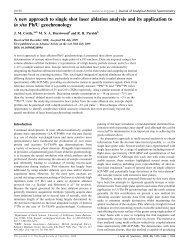
Figure 1. SRTM shaded-relief topographic rendering of the Kamchatka Peninsula. Inset shows a
higher-resolution view of the boxed area, with a different color table to emphasize geomorphic features.
Large image is 638 1113 km; inset is 93 106 km; north is up. Jet Propulsion Laboratory images
PIA03314 and PIA03374. Courtesy NASA/JPL-Caltech.
2of33

RG2004
Farr et al.: SHUTTLE RADAR TOPOGRAPHY MISSION
RG2004
to the ground surface in those areas. In addition, smooth
surfaces such as calm water and smooth sand sheets may
not scatter enough radar energy back to the sensor and thus
may not yield a height measurement.
1.2. Genesis of SRTM: The Shuttle Imaging Radar
Program
[7] When the space shuttle became operational, it ushered
in a new era of conducting remote sensing missions from
low Earth orbit aboard a reusable spacecraft that had
onboard accommodations unlike any spacecraft that had
flown before. On its flight in 1981 the shuttle carried the
first science payload, OSTA-1 (Office of Space and Terrestrial
Applications-1), including a synthetic aperture radar,
designated Shuttle Imaging Radar-A (SIR-A). The SIR-A
instrument was a singly polarized (horizontal send and
receive (HH)) L band (23.5 cm wavelength) SAR with a
fixed look angle of 45° off nadir [Elachi et al., 1982].
[8] SIR-B, which flew on Challenger mission 41-G
(5–13 October 1984), was the next step in the evolution of
shuttle-borne radars. System upgrades included a foldable
antenna with the addition of a mechanical pointing system
that allowed the beam to be steered over a look angle range of
15° to 60°. Like its predecessor, SIR-B operated at L band
and was HH polarized [Elachi et al., 1986].
[9] SIR-C was proposed as a development tool to address
the technical challenges posed by a multifrequency, multipolarization
SAR with wide-swath capability. After considerable
study and development through much of the 1980s
the SIR-C instrument evolved into SIR-C/X-SAR, an L
band and C band (5.6 cm) fully polarimetric radar with
electronic scanning capability, coupled with an X band
(3.1 cm) single-polarization (vertical send and receive
(VV)) mechanically steered radar supplied by the German
Aerospace Center (Deutsches Zentrum für Luft- und
Raumfahrt (DLR)) and the Italian Space Agency (Agenzia
Spaziale Italiana (ASI)). SIR-C/X-SAR flew as the Space
Radar Laboratory (SRL) in April and October 1994 [Evans et
al., 1997; Jordan et al., 1995]. SRL-1 and SRL-2 gathered
images over predesignated target sites and exercised several
experimental SAR techniques. Among the SIR-C/X-SAR
experiments were successful demonstrations of repeat-pass
interferometry, where images of a target were obtained on
repeat orbits (the difference in positions on each pass
forming the interferometric baseline) [Fielding et al.,
1995; Coltelli et al., 1996; Rosen et al., 2000],
and ScanSAR, where radar beams were electronically
steered in elevation to increase the swath width. ScanSAR
interferometric operations were the basis of the SRTM
topographic measurement scheme.
1.3. SRTM Objectives and Performance Requirements
[10] The Shuttle Radar Topography Mission, flown on
Space Shuttle Endeavour in February 2000 (STS-99), was a
joint project of the National Aeronautics and Space Administration,
the National Geospatial-Intelligence Agency
(NGA) (formerly National Imagery and Mapping Agency
(NIMA)) of the U.S. Department of Defense (DOD), and
DLR [Farr and Kobrick, 2000; Werner, 2001]. DLR
worked in partnership with ASI. The SRTM objective was
to acquire a digital elevation model of all land between
about 60° north latitude and 56° south latitude, about 80%
of Earth’s land surface. In quantitative terms the cartographic
products derived from the SRTM data were to be sampled
over a grid of 1 arc sec by 1 arc sec (approximately 30 m by
30 m), with linear vertical absolute height error of less than
16 m, linear vertical relative height error of less than 10 m,
circular absolute geolocation error of less than 20 m, and
circular relative geolocation error of less than 15 m. The
relative height error of the X band SRTM data was to be less
than 6 m. All quoted errors are at 90% confidence level,
consistent with National Map Accuracy Standards (NMAS).
These specifications are similar to those of the 30-m DEMs
produced by the U.S. Geological Survey as part of the
National Elevation Dataset (NED) [Gesch et al., 2002].
NED was produced by photogrammetric reduction of
stereo air photographs yielding generally a representation
of the elevations of the ground surface even beneath
vegetation canopies. As discussed in section 5.1.7, the
SRTM radars were unable to sense the surface beneath
vegetation canopies and so produced elevation measurements
from near the top of the canopies.
1.4. Mission Overview
[11] SRTM employed two synthetic aperture radars, a
C band system (5.6 cm, C radar) and an X band system
(3.1 cm, X radar). NASA’s Jet Propulsion Laboratory (JPL)
was responsible for C radar. The DLR with Astrium
(formerly Dornier Satellitensysteme, GmbH), its contractor
for the X band space segment, was responsible for X radar.
The operational goal of C radar was to generate contiguous
mapping coverage as called for by the mission objectives.
X radar generated data along discrete swaths 50 km wide.
These swaths offered nearly contiguous coverage at higher
latitudes [Foni and Seal, 2004].
[12] X radar was included as an experimental demonstration.
As it did not employ ScanSAR, the X band radar had a
slightly higher resolution and better signal-to-noise ratio
(SNR) than the C band system. Thus it could be used as an
independent data set to help resolve problems in C radar
processing and quality control [Hoffmann and Walter, 2006].
[13] The SIR-C/X-SAR interferometric experiments,
along with numerous repeat-pass interferometry results
from Seasat [Zebker and Goldstein, 1986] and the European
Remote Sensing Satellite (ERS) missions [e.g., Attema,
1991; Zebker et al., 1994; Ruffino et al., 1998; Sansosti et
al., 1999] showed that regional topographic mapping is
possible using the repeat-pass technique but that inherent to
repeat-pass radar interferometry are serious limits to the
quality of the data, which then lead to difficulties in
automating the production. Among these are temporal
atmospheric changes from pass to pass, uncertainties in
the orbit of the satellite, necessitating estimation of the
interferometric geometry from the data themselves, and
decorrelation of the radar echoes from pass to pass because
of rearrangement of scatterers on the surface [Goldstein,
3of33

RG2004
Farr et al.: SHUTTLE RADAR TOPOGRAPHY MISSION
RG2004
Figure 2. Major components of SRTM. In the shuttle payload bay are the main antennas (L band was
not used) and the attitude and orbit determination avionics (AODA). At the end of the 60-m-long mast are
the secondary antennas.
1995; Massonnet and Feigl, 1995; Zebker et al., 1997]. As
evidence of these difficulties it should be noted that despite
over 12 years of worldwide acquisition of satellite data
suitable for repeat-pass interferometry, an acceptable global
DEM has not been produced using repeat-pass InSAR.
[14] The key to successful acquisition of a data set
suitable for automated production is to remove the variability
and decorrelation due to pass-to-pass observations and to
measure the interferometer baseline and other systematic
effects accurately at all times during data acquisition.
Therefore the SRTM radars were designed to operate as
single-pass interferometers, utilizing the SRL C and X band
capabilities. For single-pass interferometry operations each
of the two SRTM radars was equipped with a supplementary
receive-only antenna in addition to the main transmit/
receive antennas situated in the shuttle’s payload bay. The
supplementary antennas were placed at the end of a retractable
60-m mast (Figure 2). During the shuttle launch and
landing the mast was stowed in a canister attached to the
forward edge of the main antenna assembly.
[15] Endeavour was launched with a six-person crew
from the Kennedy Space Center (KSC) on 11 February
2000, 1744 Greenwich mean time (GMT). The nominal
altitude was chosen to be 233 km; the orbital inclination
was 57°. With this geometry the shuttle would begin
repeating in 159 orbits in about 10 days. Since individual
orbits were separated by 218 km at the equator and since,
fortuitously, the width of the ScanSAR imaging swath was
225 km, Endeavour could map the target area, the strip
between 60° north latitude (the southern tip of Greenland)
and 56° south (Tierra del Fuego), in a single cycle of 159 orbits.
[16] Following the launch, the first 12 hours of flight
were taken up by on-orbit checkout (OOCO), during which
the payload bay doors were opened, the SRTM system was
activated and checked, and the orbiter was maneuvered to
the mapping attitude. With the successful acquisition and
verification of test data, SRTM radar mapping began.
Mapping continued for 149 orbits (222.4 hours). Data were
acquired at the rate of 180 megabits per second (Mbps)
(C radar) and at 90 Mbps (X radar). Both rates were higher
than the shuttle’s down link capacity (45 Mbps). This
required the use of high-rate data tape recorders. Selected
snapshots of data necessary for near-real-time performance
assessment were down linked via the shuttle Ku band and
NASA’s tracking and data relay system (TDRS) link to JPL
in Pasadena and to the Payload Operations Control Center
(POCC) in Houston. The total SRTM raw data volume
amounted to 12.3 Tb. About 99.96% of the targeted area
was mapped by the C radar at least once (Figure 3a).
Because of the loss of 10 orbits, a few patches of land in
North America were missed. The X radar data cover about
40% of the target area (Figure 3b). Data gathering was
concluded on flight day 10. Endeavour landed at KSC on
22 February 2000, 2322 GMT.
1.5. Techniques
[17] Radars at their most basic are instruments that
measure only one dimension: the range from the radar to
a target of interest. A radar instrument mounted on a
moving platform can form two-dimensional measurements
of a target location by exploiting the Doppler frequency
shift of a given target as well as its range. This synthetic
aperture radar technique yields two-dimensional images that
are resolved in range proportional to the reciprocal of the
4of33

RG2004
Farr et al.: SHUTTLE RADAR TOPOGRAPHY MISSION
RG2004
Figure 3. Final coverage maps for the (a) C band and (b) X band systems. The radars operated virtually
flawlessly; C band imaged 99.96% of the targeted landmass at least one time, 94.59% at least twice, and
about 50% at least three or more times. Note small red areas in the United States indicating missed areas,
as well as the polar areas that could not be reached by the shuttle’s orbit. The X band system, because it
did not operate in scanSAR mode, collected 50-km swaths with gaps between them. These gaps closed up
at higher latitudes.
radar bandwidth and in azimuth equal to half the antenna
length in the direction of motion. Typically, this leads to
images from space with 5- to 10-m resolution when the
radar is operated in this conventional strip-mapping mode
[e.g., Elachi, 1988; Raney, 1998].
[18] To access the third dimension, a range difference
between two radar images is required, and this is realized
most accurately and efficiently using principles of interferometry,
Figure 4 illustrates the concept of radar interferometry.
Each radar antenna images the surface from a slightly
different vantage point. The radar is a phase-coherent
imaging system, and the phase of the radar signal encodes
the path distance to the surface and back as well as any
phase imparted by backscatter from the surface. If the
images from two antennas are acquired simultaneously
and from close enough vantage points, the backscatter phase
observed in both images from each point on the ground will
be the same. The phase difference between each image point
will then simply be the path difference between the two
measurements of the point. Assuming the position of the
two antennas (the ‘‘interferometric baseline’’) is known, the
dimensions of the interferometric triangle can be determined
accurately and so also the height of a given point (Figure 4)
[e.g., Massonnet, 1997; Madsen and Zebker, 1998; Rosen et
al., 2000].
5of33

RG2004
Farr et al.: SHUTTLE RADAR TOPOGRAPHY MISSION
RG2004
Figure 4. Geometry of the SRTM interferometer (not to
scale). The mast formed the baseline B. Measurements of
Dr, q, a, B, and h p lead to a solution for the height of the
terrain h t .
[19] A complexity involves the fact that only the path
length difference is measured, and that is measured as an
angular phase difference, which becomes ambiguous after a
full cycle of 2p radians. Thus a method for finding the
absolute phase and therefore actual path length difference is
necessary [Madsen and Zebker, 1998]. This process is
called phase unwrapping, and a number of algorithms have
been invented to optimize the process [e.g., Goldstein et al.,
1988]. Errors in phase unwrapping typically show up as
elevation jumps of tens to hundreds of meters when estimates
from one pixel to the next jump by 2p (the ambiguity
height) or tilting caused by a poor choice of absolute phase.
[20] The size of the radar antenna limits the cross-track
extent that can be illuminated by the radar. This ground
swath was about 60 km wide for SIR-C and thus for SRTM.
In order to meet the coverage requirements and complete a
global map in 10 days a width of about 225 km was needed
on each orbit of the mission. To increase the ground swath
width by a factor of about 4, SRTM employed two techniques:
(1) ScanSAR was used to roughly double the extent of
the beam, and (2) to double the coverage again, signals with
orthogonal polarizations were transmitted simultaneously,
each with a different elevation steering angle (Figure 5).
[21] Reducing the illumination time for a target on the
ground reduces the resolution; thus the swath is widened at
the cost of azimuth resolution. For SRTM’s 12-m antenna
transmitting at 5.6-cm wavelength (C band) and moving at a
speed of 7.5 km/s at a range of 300 km, the target
illumination time is roughly 0.2 s. Using only a portion of
6of33
this time, for example, a ‘‘burst’’ period of 0.05 s, to form a
synthetic aperture reduces the resolution that can be
achieved by a factor of 4.
[22] For SRTM, at least 50% of the synthetic aperture
time was needed for adequate noise performance, allowing
at most two electronically steered beams. As the intrinsic
swath width was roughly 60 km, only 120 km could be
covered by a single-polarization ScanSAR. To obtain
adequate swath width, it was necessary to utilize the
polarization capability of the SIR-C hardware. SIR-C could
simultaneously transmit horizontal and vertical polarizations
and electronically steer the horizontally polarized
beam independently of the vertically polarized beam. In
this way the horizontally polarized channel could be
operated in ScanSAR mode covering two elevation swaths,
and the vertically polarized channel could likewise be
operated in two other elevations (Figure 5).
2. MISSION DESIGN
[23] SRTM was designed to meet a particular map
accuracy specification. This stringent requirement, coupled
with the characteristics of the existing SIR-C hardware, led
to a constrained mission design space and a set of natural
design choices for the mission. The goal of a radar interferometer
is to measure the difference in range between two
observations of a given ground point with sufficient
accuracy to allow accurate topographic reconstruction. This
is done through the interferometric phase and knowledge
of the interferometer geometry (Figure 4). A simplified
expression for the target height h t is
h t ¼ h p r cos sin 1 lf
þ a ;
2pB
Figure 5. How the SRTM swaths were constructed.
C radar illuminated a 225-km swath by alternately
collecting pairs of subswaths using scanSAR. Subswaths
1 and 3 were illuminated first, then 2 and 4, etc. X-SAR was
not able to scan, so its 50-km swath was fixed between
subswaths 3 and 4.

RG2004
Farr et al.: SHUTTLE RADAR TOPOGRAPHY MISSION
RG2004
where h p is the platform height (antenna altitude with
respect to the WGS84 reference ellipsoid [Defense Mapping
Agency, 1997]), r is the range, f is the measured
interferometric phase, a is the baseline roll angle, l is the
observing wavelength, and B is the baseline length. Clearly,
errors in knowledge of the quantities in this equation impact
the total SRTM performance. The trade-off between these
errors was a large part of the mission design. For SRTM the
radar instrument provided data necessary to determine r and
f, while a metrology package (Attitude and Orbit
Determination Avionics (AODA)), described in section
3.5, measured the detailed shape of the interferometer, in
essence a, B, and h p .
[24] The allocation of the vertical error to the various
system components of SRTM was roughly as follows: phase
noise, 8 m; baseline angle, 7 m; baseline length, 1 m;
platform location, 1 m; and range 1 m. The usual
components of the radar equation, radar aperture size,
radiated power, noise properties of the receiver, range to
the target, and surface backscatter characteristics, were the
given parameters of the mission, derived from SIR-C
hardware and shuttle operations capabilities. These quantities
set the intrinsic statistical phase noise performance of
the interferometer. Given the phase noise of the system, the
height acuity of the system can be controlled by the design
of the remainder of the interferometer.
[25] The sensitivity of height to phase is given by the
derivative of the above equation:
@h
@f ¼ l 2p
r sin q
B cosðq
aÞ:
Several terms in this equation were also established outside
the design trade space. The choice of wavelength between
L band and C band for SRTM was clear: An outboard
C band antenna would have less mass and volume and was
therefore obvious for a shuttle mission that was already
pushing the limits of the vehicle’s carrying capacity. The
shuttle orbit of 233 km at 57° inclination was the highest
possible for a fully loaded shuttle. Maximizing the altitude
also maximizes the antenna footprint on the ground,
contributing to achieving full circumferential coverage in
10 days of mapping. To minimize layover effects, look
angles were chosen between 30° and 60°. These angles,
along with the altitude, set the range extent of the swath.
Thus in this sensitivity equation the only free parameters are
the interferometric baseline B and orientation angle a.
[26] As the baseline becomes larger, the sensitivity of the
height to phase noise is partially reduced. The phase noise is
dependent on the backscatter properties of the surface:
Poorly backscattering surfaces have lower SNR, with higher
phase variance. It was important to characterize the anticipated
worst-case backscatter at C band and choose the
baseline length accordingly.
[27] The baseline angle was chosen to be 45°. This angle
minimizes the sensitivity of the observation to errors in the
baseline length. Given these constraints, B was chosen as
large as necessary to meet the height noise requirement. For
a typical worst-case correlation of 0.7 and 2 looks, the phase
noise is about 0.5 radians. The baseline length must be
chosen so that after multiple observations are combined, the
height noise is within the statistical height error allocation.
For a baseline of 30 m, as was originally proposed, the
statistical height noise (subject to the other interferometric
constraints, as stated above) would be 25 m, an unacceptable
magnitude. Even with two independent observations
(ascending and descending orbits, for example) the statistical
noise would be greater than the total height error
budget of 16 m. It was determined that a 60-m baseline,
yielding a worst-case statistical height noise of 12 m, was
acceptable and would have to be accommodated in the
payload design.
[28] In order to meet the statistical phase noise allocation
of 8 m a key mission characteristic had to be at least double
coverage of every point on the Earth. Thus the 12-m worstcase
height noise could be reduced by a factor of 2 to
pffiffiffi
about 8 m. Double coverage was achieved by observing
every point on the ascending and the descending portion of
the orbit. The orbit ground track separation at the equator
was about 218 km; thus with a 225-km ScanSAR swath it
was possible to just cover all points on the ground within
the 10-day flight. Observations had to be made without
failure on both ascending and descending orbits for points
located within ±20° (latitude) of the equator. At higher
latitudes, coverage overlapped as the orbits converged, but
near the equator only one ascending and one descending
pass was available.
[29] Another possible interferometric phase error can
arise from relative phase differences between the two
receiver channels. The receivers were not identical mechanically
or thermally, and the signal path length from receiving
antenna to electronics was vastly different because of the
60-m baseline. Rather than attempt to force the receiver
phases to be identical, a calibration tone signal with common
reference was distributed to the antennas over optical
fiber cable to the deployed antenna [McWatters et al., 2001].
The signals were injected into the receive paths at the
antennas and detected in the data processing. The phase
differences did indeed vary over the life of the mission by
many degrees and would have been a significant error
source had they not been compensated for in the processing.
After compensation the error was less than 1 m.
[30] The next largest error source in the interferometer
was the baseline angle, a. The sensitivity of height error to
angle error is given by
@h
¼ r sin q;
@a
which states that an error in baseline angle amounts to a
height error @h given by the rotation of the ground range
vector to the target (r sin q) by angle @a. To meet a
height error allocation of 7 m, one must know the
baseline angle to an accuracy of 7/233000 or 3 10 5
radians (about 6 arc sec).
7of33

RG2004
Farr et al.: SHUTTLE RADAR TOPOGRAPHY MISSION
RG2004
Figure 6. Mast motions induced by shuttle thruster firings (arrows) during data take 72.10 (flight day 4).
(a) Displacement of mast tip as a function of along-track distance. Note maximum displacement of about
10 cm and the rapid damping. The fundamental period of the mast was about 8 s. (b) Shuttle roll angle as
a function of along-track distance. Note gravity-gradient torque causing increase in roll angle between
thruster firings. Shuttle dead band was approximately 0.3°.
[31] For a system where the baseline is slowly drifting,
one can imagine a calibration scheme where any drifts in the
baseline angle are removed by ground control points spread
throughout the world. Indeed, the mission design stipulated
that the data takes begin over the ocean prior to landfall and
end over the ocean after mapping the land to deal with the
possibility of long-term drifts. (It turned out that there was
very little long-term drift.) However, as Figure 6 illustrates,
the shuttle is a dynamic, mechanically oscillating system.
Because thrusters were firing periodically to maintain the
shuttle attitude, the mast resonated and oscillated. This
resulted in a displacement of as much as 10 cm for the tip
of the mast and a change of several tenths of degrees in the
shuttle attitude. A few ground control points were therefore
insufficient to determine the baseline. The metrology package
(AODA) continuously measured the position and attitude
of the shuttle and the outboard antennas to the required
accuracy.
3. SRTM SYSTEM
3.1. SRTM Hardware and System Overview
[32] The SRTM architecture was based on the SRL SIR-
C/X-SAR instruments, modified and augmented to enable
single-pass interferometric operations. The resulting new
system consisted of four principal subsystems: the C band
synthetic aperture radar (C radar), the X band synthetic
aperture radar (X radar), the antenna/mechanical system
(AMS), andtheAODA. Ofthefourmajorsubsystems, Cradar,
X radar, and AMS utilized the well-tested SIR-C/X-SAR
hardware. AODA was a newly developed subsystem.
Substantial parts of AMS were also new. The unique
concepts on which AODA was built and AMS was
modified contributed substantially to the almost flawless
execution of SRTM.
[33] Owing to its bulk and complexity the SRTM hardware
took up all of the shuttle’s cargo space (Figure 7).
SRTM hardware was placed in the payload bay (Figure 8),
in the middeck, and on the aft flight deck (AFD) (Figure 9).
Hardware located in the AFD included three payload highrate
recorders (PHRRs), tape cassettes, digital data routing
electronics (DDRE), recorder interface controller (RIC), and
AODA processing computers (APC). The middeck hardware
included two spare PHRRs, spare power supplies,
spare computers and hard drives, spare cables, repair kits,
and tape cassettes. A total of 350 cassettes were flown. A
warm spare PHRR was carried in the middeck accommodation
rack. The total mass of the SRTM payload was
13,600 kg.
3.2. C Radar Subsystem
[34] While much of the radar system was inherited from
SIR-C, several new systems or modifications were necessary
for interferometric operation: C band receive-only
outboard antenna panels (supplied by the Ball Corporation),
the beam autotracker (BAT) (Ball Corporation), and the
calibration (CAL) optical receiver (COR). The elements of
C radar located in the crew cabin were the DDRE unit,
which multiplexed the high-rate data streams from C radar
and X radar onto the PHRRs, under the control of the RIC
(Figure 9). RIC was a laptop computer with software to
handle all the faults and unusual recording situations that
were encountered on SRTM. RIC received simple commands
from the command timing and telemetry assembly,
and it monitored the PHRRs to make sure that the commands
were executed properly. It had an elegant new
feature: the ability to calculate the moment when a data
take would exceed the remaining tape capacity. It would
then start up the second recorder in time for it to capture the
data as the first recorder ran down. The overlap was such
that the same data were recorded on both PHRRs for about
8of33

RG2004
Farr et al.: SHUTTLE RADAR TOPOGRAPHY MISSION
RG2004
Figure 7. SRTM hardware in Endeavour’s payload bay in mapping attitude. Nearest foreground is the
space station docking adapter. Next is the mast canister with the partner logos. Note mast with many
cables running its length. Main antenna is beyond canister. X-SAR antenna is on its right edge; C band
antenna is at the left edge. The pyramidal object in the middle of the main antenna is AODA covered with
thermal blankets. Johnson Space Center photograph s99e5476.
30 s. The astronauts were kept busy loading and unloading
C radar tapes; the capacity of a single tape was 20 min at the
C radar data rate. DDRE also had the ability to route realtime
data or tape playback to the shuttle’s Ku band signal
processor (KuSP). The KuSP was a link to JPL and the
POCC via TDRS, the White Sands Ground Terminal, and
DomSat.
Figure 8. SRTM hardware in shuttle payload bay. (top) Stowed configuration. (bottom left) Deployed
Outboard Antenna System. (bottom right) Details of the AODA support panel.
9of33

RG2004
Farr et al.: SHUTTLE RADAR TOPOGRAPHY MISSION
RG2004
Figure 9. Mission Specialists Gerhard Thiele and Janet Kavandi go over the crew timeline in the shuttle
aft flight deck. The laptop at top left is the recorder interface controller; its screen shows the status of
three payload high-rate recorders (PHRR). Behind Thiele’s arm are two PHRRs. Johnson Space Center
photograph sts099_327_003.
[35] C radar incorporated an interesting design feature:
the beam autotracker. The concept of BAT, first tested on
JPL’s airborne SAR (AIRSAR) test bed, seemed simple:
Split the antenna into right and left beams, compare the
signal strength in each, and then change the antenna pattern
to equalize the signal strength. This electronic beam steering
could compensate for rapid motions of the mast. The AIR-
SAR test showed that at least in some situations the concept
worked. Fortunately, the mast proved to be quite stable over
a data take, and thus BAT was not used.
3.3. X Radar Subsystem
[36] The 12-m-long and 40-cm-wide X band main transmit
and receive antenna was mounted to the C band radar
antenna truss structure in the shuttle cargo bay and mechanically
tilted to 7° (59° off nadir), placing its 50-km beam
between C radar beams 3 and 4 (Figure 5). The X-SAR
main antenna and electronics were left nearly unmodified
from the SRL missions. The new outboard receive antenna
was only 6 m long, consisting of six 1-m panels (spare parts
from SRL). It was mounted together with the X band
outboard electronics to the outboard antenna support structure.
On the backside of the six antenna panels, six lownoise
amplifiers were attached, one for each panel. Together
with the six controllable phase shifters, this enabled electronic
beam steering of the outboard antenna within a range
of ± 0.9° in azimuth. The electronic pointing capability was
designed for dynamic pointing based on the BAT signal to
stay within the illuminated spot on the ground, but it was
only used to correct for a slight static misalignment of 0.1°
between the main and secondary antennas detected during
OOCO.
3.4. Antenna/Mechanical System
[37] The SRTM mechanical system was based on the
SIR-C/X-SAR system, with significant changes. The SIR-
C/X-SAR instrument flew one row of 18 C band panels and
two rows of 9 L band panels. SRTM retained the 18 C band
panels and 6 of the L band panels, but since the L band
system was not used, the superfluous panels were removed
to save weight.
[38] The most significant SRTM hardware addition was
the Outboard Antenna System (OASYS) and its deployment
system. The OASYS consisted of outboard support struc-
10 of 33

RG2004
Farr et al.: SHUTTLE RADAR TOPOGRAPHY MISSION
RG2004
ture (OSS), outboard C band panel array, outboard X band
panels and electronics, and AODA equipment (Figure 8).
The total weight of the OASYS was 397 kg. The OASYS
deployment system included four major components: the
60-m mast and mast canister, a mast damping system, an
OASYS flip hinge, and an OASYS static pitch and yaw
attitude adjustment mechanism referred to as the ‘‘milk
stool.’’
[39] The mast, manufactured by AEC-Able Engineering,
Inc., of Goleta, California, derived from the International
Space Station solar array blanket support structure. The
mast was a truss structure consisting of 86 bays plus the
milk stool. Nominally, it took approximately 20 min to
extend or retract the mast. The mast longerons and battens,
longitudinal and transverse members, respectively, were
pultruded graphite/epoxy rods. The mast diagonals were
made of titanium wire rope. Four ribbon cables, two fiber
optic cables, eight coaxial cables, and one nitrogen gas line
ran the length of the mast (Figure 7). An orderly folding
scheme assured that the cables stowed in a repeatable,
compact shape. An extravehicular activity (space walk) to
manually crank the mast if it failed to extract or retract was a
part of the mission plan. The crew also had the option of
jettisoning the canister/mast assembly. The mast canister
was mounted to the forward end of the antenna core
structure (ACS). In launch configuration the outboard
antenna was folded across the top of the canister and the
inboard antenna (Figure 8). The OASYS flip hinge rotated
the OASYS 180° from its stowed postion to its deployed
position once the mast was deployed. The mast damping
mechanisms were designed to achieve greater than 10%
damping ratios in the first bending mode and the first
torsional mode. The static OASYS pitch and yaw attitude
was adjusted to align the outboard and inboard antennas via
the milk stool during OOCO.
[40] The combination of the mast and the outboard
antenna attached to the mast’s tip represented a momentum
arm extending from the shuttle. The arm was not accounted
for by the shuttle’s regular attitude control system. For
mapping the mast had to point sideways, 45° relative to
the nadir vector. The corresponding shuttle attitude would
then be 59° from the bay-down orientation. The off-vertical
pointing exposed the shuttle/mast system to a gravitygradient
torque. Anticipating this, a cold gas thrust system
was added to OAS, with the purpose of providing a
compensating torque. This was calculated to reduce the
frequency of the shuttle’s thruster firings, thus conserving
propellant. On flight day 2 it was determined that orbiter
propellant usage had doubled from 0.07% to 0.15% an hour.
The increase was caused by the failure of the cold gas thrust
system due to a burst diaphragm.
[41] Correct pointing of the mast held the key to successful
interferometric operations of the SRTM radars. Errors in
pointing would lead to misalignment of inboard and outboard
antennas and to the loss of interferometric capability.
Apart from affecting the consumables budget the attitude
control system firings had an additional consequence in that
they triggered dynamic responses by the mast. Gravity
unloading, load shifts during the launch, and preflight
assembly and alignment errors resulted in a quasi-static
pointing bias. In-flight, thermal deformation of the mast and
antenna structure created pointing errors with time constants
of several minutes. (The mast’s primary modal frequency
was on the order of 0.1 Hz.) Although the pointing
challenges were mitigated by the SRTM structural and
mechanical design, the mast pointing errors had to be
measured continuously by AODA and compensated for
by the radar instruments and the ground data processing
system.
3.5. Attitude and Orbit Determination Avionics
[42] The primary function of the AODA system was to
provide a postflight time history of the interferometric
baseline for use in the topographic reconstruction processing
[Duren et al., 1998]. For SRTM, AODA was required to
provide estimation of the interferometric baseline length,
attitude, and position to an accuracy of 2 mm, 9 arc sec, and
1 m (at 90%, or 1.6 sigma, confidence level), respectively.
These requirements had to be satisfied throughout the entire
mission whenever the radars were collecting data at a rate
better than 0.25 Hz. During instrument development, however,
AODA took on the additional requirement to support
mission operations, including verification of in-flight mast
deployment, antenna alignment, and shuttle attitude control
optimization.
[43] Safety demanded that proper deployment of the mast
be verified before the mapping phase of the mission. For
instance, if one or more of the mast latches did not snap into
place when the mast was extended, the structure might still
have appeared unimpaired but would have collapsed when
the shuttle thrusters fired. Endeavour remained in free drift
in a stable gravity-gradient attitude during mast deployment
and verification. AODA measurements of errors in the
deployed mast tip position and attitude allowed the crew
and ground teams to verify mast integrity before engaging
shuttle’s attitude control system.
[44] The inboard and outboard antennas needed to be
aligned in such a manner that the radar antenna beam
patterns on the ground had maximum overlap. Roll misalignment
was less critical because the beam width about
the roll axis was relatively large, but errors about the pitch
and yaw axes could not exceed 0.06° [Geudtner et al.,
2002]. Following mast deployment, the astronaut crew used
AODA measurements to guide static alignment adjustments
in yaw and pitch utilizing the milk stool mechanism.
[45] Though preflight (1-g environment) estimates of
mast modal frequencies were available, in-flight measurement
was preferred. Since notch filter settings in the
shuttle’s attitude control system could be selected to reduce
mast response, errors in preflight estimates could result in
inefficient on-orbit performance, i.e., excessive attitude
control response and correspondingly excessive propellant
use and mast motion. The consequence of nonoptimal
propellant use could be a shortened mission. It turned out
that this in-flight identification was crucial because the
11 of 33

RG2004
Farr et al.: SHUTTLE RADAR TOPOGRAPHY MISSION
RG2004
passive damper at the root of the mast failed to function in
flight.
[46] The AODA system consisted of a flight segment and
a ground segment. The central part of the flight segment
was the AODA support panel (ASP), kinematically
mounted to the inboard ACS, in place of one of the removed
L band panels (Figures 7 and 8). The ASP furnished an
isothermal, optical-bench-type support for the following
AODA sensors: star tracker assembly (STA), inertial reference
unit (IRU), Advanced Stellar and Target Reference
Optical Sensor (ASTROS) Target Tracker (ATT), and electronic
distance meters (EDMs). With the exception of the
STA this hardware consisted of inherited or commercial
equipment in order to keep the cost low. AODA was
necessary because the standard shuttle guidance and navigation
system did not offer the required accuracy and
because significant thermal distortions existed between the
shuttle guidance platform and the SRTM inboard antenna.
[47] The baseline attitude had two primary components:
the inertial platform or inboard antenna attitude and the
(primarily) mast-induced relative motion between the two
radar antennas. The inertial platform attitude was measured
by STA and IRU. STA consisted of a Lockheed Martin
autonomous star tracker (AST-201) instrument. The IRU
was a Teledyne dry rotor inertial reference unit (DRIRU-II).
The IRU measurements were useful in refining the attitude
estimates during the postflight ground data processing. The
ATT was critical for meeting four AODA requirements:
baseline determination, antenna alignment, mast deployment
verification, and mast modal identification. Developed
by JPL in the 1980s as a high-precision star tracker for
planetary missions, ASTROS required extensive modifications
for use by SRTM. ATT tracked three red light-emitting
diode (LED) targets (Optical Target Assembly (OTA))
located on the outboard antenna and separated by 1 m both
laterally and in line of sight (Figure 8). AODA determined
the outboard antenna’s relative attitude and position based
on the centroid information collected by ATT on all three
OTA targets.
[48] Although the ATT provided good accuracy in determining
5 of the 6 outboard antenna degrees of freedom, it
had degraded range accuracy because of OTA geometrical
constraints imposed by the outboard antenna dimensions.
Late in the AODA design phase it was deemed necessary to
add an instrument capable of accurately measuring the
baseline length, i.e., the range to the outboard antenna. A
commercially available surveying rangefinder, Leica-Wild
DI2002 EDM, satisfied the AODA requirements [Duren
and Tubbs, 2000]. Four modified and flight-qualified units
were utilized: two units to measure range to the outboard
antenna and the other two units to measure displacements
between the inboard C and X band arrays (each measuring
one leg of a triangle to solve for X and Z displacement). The
EDM outboard target was an array of cube corner-reflectors
placed along the inboard edge of the outboard antenna. This
arrangement allowed the two outboard-looking EDMs to
acquire signal even in the event of large mast excursions. In
addition, a single cube corner reflector was placed on the
inboard X band antenna.
[49] Orbit (platform position and velocity) determination
was provided by an onboard GPS consisting of two P code
tracking GPS Receivers (GPSRs) developed as part of JPL’s
TurboRogue Space Receiver Program [Duncan et al.,
1998]. The onboard receiver position solution, via ‘‘direct
GPS’’ technique, is limited to 10- to 100-m accuracy. To
obtain the required 1-m position determination, the pseudorange
and phase observables acquired by the onboard
GPSRs were combined with those simultaneously available
from the existing ground network of globally distributed,
well-surveyed GPS receivers. Such an approach could be
termed a ‘‘global differential GPS’’ technique [Bertiger et
al., 2000].
[50] Two laptop computers with JPL-developed software
served as the onboard AODA workstations (APCs). Located
in the shuttle’s aft flight deck (Figure 9), the APCs were
heavily relied upon during OOCO. They fulfilled several
functions, in particular, guiding antenna alignment and
providing control loops for operating ATT and EDM. The
AODA system was designed to operate and record autonomously
once the mapping phase of the mission began.
[51] The AODA ground segment consisted of the global
network of ground GPS receivers, the GPS Inferred Positioning
System (GIPSY), the AODA Ground Data Processor
(AGDP), and the AODA Telemetry Monitor/Analyzer
(ATMA). The ground segment was used during the mission
to support antenna alignment, mast modal identification,
and quick-look height reconstruction. AGDP took the raw
data from ATMA (or APCs, following postflight recovery),
performed the attitude and baseline determination, recombined
the GIPSY output data, and presented the radar
processor ground segment with a single time-tagged data
archive.
4. MISSION OPERATIONS
4.1. Orbit Maintenance
[52] In order to meet the mission requirements and to
comply with shuttle operational constraints the orbit selected
was circular, 57° inclined, with a mean altitude of 233.1 km.
This orbit repeated the same ground track in 9.8 days after
159 revolutions. It produced ground tracks spaced at
218 km, measured orthogonal to the direction of travel, or
at 252 km, measured along the equator. Since C radar had a
mean swath width of 225 km, the nominal overlap was only
7 km. Premission simulations had shown that orbit drift due
to atmospheric drag would amount to about 1.5 km/d at the
equator. Perturbations caused by drag on the 60-m mast and
outboard antenna were difficult to quantify. Even so, it was
evident that unless compensated for, the orbit drift would
cause loss of swath overlap in about 24 hours. To prevent
orbit decay, extremely precise control had to be designed
into the mission. This control was exercised by a series of
nonstandard orbit trim maneuvers, known as ‘‘fly cast’’
maneuvers, executed at a nominal frequency of one per day.
12 of 33

RG2004
Farr et al.: SHUTTLE RADAR TOPOGRAPHY MISSION
RG2004
[53] The first of a series of ‘‘fly cast’’ maneuvers was
performed on flight day 2. The fly cast maneuver was
designed to reduce strain on the mast during the daily orbit
boost maneuver. The shuttle, which flew tail first during
mapping operations, was moved to a nose-first attitude with
mast extending outward. A brief pulse began the maneuver.
The mast deflected backward, and when it reached maximum
deflection, the main burn was performed, pinning the
mast. After the burn the mast returned forward. As it
reached the vertical, another pulse was applied, arresting
the mast’s motion.
[54] The failure of the cold gas thruster at the tip of the
mast constituted the most significant obstacle in flight.
Without the thruster’s counteraction of gravity gradient
torques on the orbiter plus mast the shuttle used up much
more propellant than planned for attitude control, reducing
the amount of propellant available for orbit maintenance. In
order to complete mapping with the reduced amount of
propellant, shuttle navigators and the SRTM mission planners
worked out a new maneuver sequence for orbit trim
burns 6–9. Trim burns 8 and 9 were deleted, the Dv of trim
6 and 7 was increased, and trim 7 was postponed by about
12 hours. The operations team selected a phasing and choice
of Dv that were creative enough to cause no gaps to open up
between radar swaths. Therefore it was possible to successfully
complete mapping operations without significantly
impacting the end results.
4.2. Ground Operations
[55] The complexities involved in securing proper interferometric
performance on the part of the SRTM radars
required participation by both the astronaut crew and
dedicated ground teams. The crew controlled pallet and
antenna activation and deactivation, initial antenna alignment,
and tape change outs. The SRTM ground teams,
located at the Payload Operations Control Center at NASA’s
Johnson Space Center (JSC), the Customer Support Room
at JSC, and the Mission Support Area (MSA) at JPL,
controlled the rest of the SRTM activities. Each of the
two SRTM radars was operated by a separate system
centered at the POCC. Operations of C radar were handled
by the Mission Operations System (MOS), and those of X
radar were handled by the Mission Planning and Operations
System (MPOS). The JPL MSA, networked to the POCC,
was responsible for processing C radar data down linked
from the shuttle during the mission. DLR had a similar
system set up in Germany. The down link connection to JPL
was routed through the NASA Tracking and Data Relay
Satellite System and the White Sands Ground Terminal,
while a separate high-rate data link was used to transmit
processed images and measurements to JSC.
[56] Characterized in the most general terms, the operating
systems for C radar and X radar performed parallel and
equal tasks: mission planning, instrument commanding,
instrument health monitoring, and instrument and system
performance analysis. A brief description of MOS as the
representative of both systems should thus suffice. Referring
to Figure 10, note that MOS consisted of six major
subsystems: Mission Planning Subsystem (MPS),
Command Management Subsystem (CMS), Telemetry
Management Subsystem (TMS), Performance Evaluation
Subsystem (PES), Data Management Subsystem (DMS),
and ATMA. The Mission Planning Subsystem generated
orbit predictions, performed SRTM long- and short-term
planning, and produced mission timelines and C radar
command inputs. Generation of ephemerides was done
utilizing the Orbiter state vectors received from the Mission
Control Center (MCC) every 2–3 orbits. Using these, MPS
planned the start and stop times of each data take. Further,
using a low-resolution DEM, it computed the distance to the
surface of the Earth during mapping. By knowing this
distance, MPS could select the appropriate set of radar
parameters. The C radar mission timeline was produced
every 6 hours and was sent to MPOS with the goal of
generating X radar timelines and commands. MPS then
added PHRR playbacks and other C radar and X radar
events to the data take timeline. The finished mission
timeline was provided to the MCC planners for crew flight
plan inputs; it was also forwarded to the SRTM Customer
Support Room and to the JPL MSA.
[57] On the basis of the mission timeline, MPS generated
the C radar command input file. Using the command input
files produced by MPS, the CMS generated time-tagged
commands for uplink to C radar. CMS also had the
capability to generate immediate (real time) commands. In
addition, CMS received AODA block commands and
formatted them for uplink to the AODA flight instruments.
The TMS could be viewed as the CMS downlink counterpart.
TMS decommutated the Orbiter operational downlink
telemetry and split it into the C radar, AODA, Orbiter
instrumentation, and Orbiter Systems Management data
streams. The all-important AODA stream was routed to
the ATMA in the POCC. Commands were sent to the
onboard instruments via MCC and the S band link to the
orbiter subsystems. Instrument telemetry was received over
the same link. Last, the PES evaluated the single-channel
and double-channel (interferometric) performance of the
C radar instrument during the mission and, in conjunction
with MPS, provided orbit-by-orbit reports of those data
takes that failed to meet the mission requirements. PES also
monitored beam alignment as measured by the AODA
instruments, the (unused) C radar BAT, the JPL Radar
Verification System (RVS) at the JPL MSA, and the echo
profile information from both C radar and X radar. PES
coordinated inboard/outboard antenna adjustments using the
milk stool, and it performed steering of the inboard and
outboard antennas. PES tools were used to predict echo
strength, thermal noise, range and azimuth ambiguity levels,
and relative height error and to monitor gain settings, swath
overlap, and BAT alignment. The accuracy and stability of
the alignment and the mast dynamics experienced throughout
the mission was less than 0.025° and was better than
expected. No dynamic steering of the secondary antenna
beam with the BAT was necessary.
[58] At calibration sites in southern California, northwestern
Australia, and near Munich, Germany, radar corner
13 of 33

RG2004
Farr et al.: SHUTTLE RADAR TOPOGRAPHY MISSION
RG2004
Figure 10. SRTM Mission Operations System. Johnson Space Center (JSC) Mission Control Center
was the main interface to the shuttle for C radar Mission Operations System and X radar Mission
Planning and Operations System in the Payload Operations and Control Center (POCC) at JSC (central
part of diagram). JPL Mission Support Area processed C radar data and returned results to POCC via
tracking and data relay system.
reflectors were deployed, and ground truth data were
acquired. The alignment between the C band and X band
radar systems was verified, and the azimuth antenna
patterns were measured with radar receivers during the
passes over the German calibration site.
[59] During the SRTM mapping phase of 222.4 hours,
C radar operated for 99.2 hours, and X radar operated for
90.6 hours. A total of 765 data takes were executed. Of
these, 399 were C radar only, 1 was X radar only, and
365 were simultaneous C and X radar. Classified by their
purpose, 674 data takes were over land, 30 calibration data
takes were over ocean, and 61 data takes were dedicated to
equipment testing. The number of high-density tapes used
was 330 (208 for C radar data, 122 for X radar data).
The volume of data produced by SRTM, 12.3 Tb (8.6 Tb by
C radar, 3.7 Tb by X radar), compares to the capacity of the
Library of Congress.
[60] After Endeavour landed at KSC, the flight tapes
were unloaded and formally handed over to the C radar
and X radar ground processing teams. Over the subsequent
8 weeks the tapes remained at KSC while teams separated
and transcribed the raw C and X band data to secondary sets
of tapes. These secondary tapes were the ones that were
eventually used for DEM processing, while the flight tapes
were shipped to a secure archival facility for safekeeping.
4.3. Real-Time Analysis
[61] The data down linked during the mission were
processed as soon as they were received, allowing a near
real-time look at the quality of the data and a chance for new
discoveries. Real-time down links would only accommodate
one channel, so no real-time tests of the full interferometric
capability were possible. However, tape playbacks
at reduced speed allowed full interferometric processing to
DEMs for both the C and X band systems. It was apparent
immediately that in those parts of the world where highquality
cartographic coverage was sparse the SRTM data
brought a vast improvement. This bolstered confidence in
the performance of the SRTM engineering systems and
demonstrated the value of the rapid processing of the down
linked data. By the time the Endeavour flight ended,
mission personnel knew that a new topographic data set
of great depth and richness had been acquired.
5. DATA PROCESSING
[62] Except for early comparative analysis of performance
for the purpose of fine tuning the AODA solutions
the C radar and X radar data were processed independently.
The processing systems, developed on either side
of the Atlantic, shared many general characteristics, but
the details of the algorithms and implementations varied
greatly. For example, the multibeam ScanSAR interferometric
approach that C radar needed to cover the globe
required a specialized burst-mode processor [Holzner and
Bamler, 2002]. The X radar acquired data in a single
beam in a continuous strip at the expense of limited
coverage. Other differences arising from the coverage
issues are described below.
14 of 33

RG2004
Farr et al.: SHUTTLE RADAR TOPOGRAPHY MISSION
RG2004
Figure 11. SRTM processor. Three main subsystems processed SRTM data to DEMs: data transfer,
topography processor, and mosaicker. Calibration and validation (Q/A) contributed to several parts of the
processor.
5.1. C Radar Algorithms
[63] The approach to reducing nearly one trillion paired
pulse echoes of radar data to a continentally seamless digital
elevation model, accurate to about two parts in 10 5 , involved
reliance upon years of experience in the development of radar
interferometry algorithms for airborne and spaceborne topographic
mapping applications. Some of the SRTM algorithms
were simple adaptations to the space environment of airborne
single-pass approaches. Others required significant rework
and innovation. Figure 11 shows the overall algorithmic flow
for C radar processing. Motion and telemetry data were
resampled to a uniform grid that was tailored to each data
take and latitude band. The preprocessed data were then
processed to elevation data mapped to a locally spherical
coordinate system. The freshly processed data were immediately
checked for quality against existing topographic
databases. Passing that test, they were entered into an archive
as the data takes for a continent were accumulated. When all
the data take processing was completed for a continent, the
data were further manipulated and adjusted to produce a
seamless, self-consistent equiangular elevation model for the
continent. The model was tied down at the coasts by wellknown
ocean heights corrected for tidal effects. The continental
data were validated, error statistics generated, and then
segmented into 1° 1° cells for distribution.
5.1.1. AODA Processing
[64] As described in section 3.5, the AODA system and
data were a key aspect of the interferometer. Reduction of
the data to give position and velocity of the shuttle and a
time-varying baseline vector involved the blending of data
from systems with different time bases, sampling rates, and
latencies. Very small errors in sampling or delay could cause
large errors in the final height map; these errors were not
easily removed because biases were not fixed. This is both a
curse and blessing: Uncompensated errors could be large,
but given the large amount of reference ocean data, it was
fairly straightforward to sort out errors.
[65] AODA data reduction algorithms were extensions of
well-established navigation solutions developed at JPL for
deep space missions. While planetary spacecraft rarely
experience the dynamic environment of the shuttle, a Kalman
filtering approach was easily tailored to it [Wong et al.,
2001; Duren et al., 1998]. Instrumental effects in the
cameras, saturation of the LEDs, blinding of the star
cameras due to shuttle wastewater dumps, etc., required
prefiltering of the data, including some editing by hand.
[66] GPS processing using GIPSY was carried out on
overlapping orbit arcs. Self-consistency of the solutions was
checked in the overlap regions, and agreement to better than
1 m was found in general.
5.1.2. Low-Resolution and Calibration/Validation
Databases
[67] The assembly of databases that could be used to aid
the processing and serve as the calibration and validation
points was an important component of preparation for the
processing. A full report on SRTM calibration and valida-
15 of 33

RG2004
Farr et al.: SHUTTLE RADAR TOPOGRAPHY MISSION
RG2004
tion has been presented by Rodriguez et al. [2005], and a
condensed version is available [Rodriguez et al., 2006].
This activity spanned nearly the entire period of instrument
development; it involved active coordination with NGA and
their international partner agencies for data sharing and new
ground truth acquisitions. In particular, the following data
sets were assembled:
[68] 1. A global digital elevation model, composed of the
best digital elevation data available up to Digital Terrain
Elevation Data (DTED-1) was generated with a 500-m post
spacing. The purpose of these data was to aid the topographic
processor in deciding what the approximate local
height actually was and as a first check of topographic
quality of the processor product. Tidally variable ocean
heights formed an important part of the initialization of the
data take processing. Since ocean heights varied over the
duration of the mission, a static DEM was of little use.
Instead, for each data take a tailored DEM was generated
consisting of the static heights over land and tidally adjusted
TOPEX/Poseidon–derived ocean heights.
[69] 2. Ground control points were derived from NGA
historical data, offering accurate heights at several thousand
points (specified by their latitudes and longitudes) around
the world. These points could be used in either calibration
of the data or validation of the final product (but not both).
[70] 3. Kinematic GPS data were acquired by driving an
appropriately equipped GPS receiver across nearly every
continent, north to south and east to west. The goal was to
provide validation data and characterization of the spatial
spectrum of height errors in the data.
5.1.3. Time-Varying Parameter Files
[71] The Earth’s surface was divided into latitude bands
where, for geometric convenience, the ellipsoidal shape of
the Earth could be well approximated by a sphere. A
complete data take would extend from ocean to ocean and
would be divided into as many latitudinally controlled
segments, called peg regions, as required. A peg region
was defined by a single latitude, longitude, and heading
known as the peg point, from which the coordinate transformation
(and its inverse) from a spherical radar mapping
coordinate system to the cartographic system is described
analytically [Madsen and Zebker, 1998]. The output topographic
map (as well as radar brightness and statistical error
image products) was represented in this spherical system.
[72] Time is usually the independent variable against
which other sensor quantities are characterized. However,
once the geometry of the peg region was established, it
became more convenient to describe the position along the
spherical arc in the local coordinate system as the independent
variable. This position is related to time through the
spacecraft velocity, but a uniform time grid does not
necessarily lead to a uniform spatial grid since the velocity
may change with time. All parameters needed for tying the
radar pulse data to the parameters of the instrument,
including time, cross-track position, velocity, interferometric
baseline, and radar mode changes (among others), were
resampled in order to be placed on this uniform spatial grid.
This approach greatly simplified the algorithmic logistics.
The grid was spaced at precisely 20 m, matched to the
intrinsic along-track resolution obtainable from each burst.
5.1.4. Topographic Processing of Radar Data
[73] With the availability of the preprocessed motion and
auxiliary radar mode data and low-resolution databases, it
was possible to develop a processor that began processing at
the beginning of a data take, typically over ocean, and
ended at the end of a data take. Furthermore, the processor
software was written to allow continuous processing
through a data take, even if the data take spanned more
than one peg region. Special algorithms were included to
overlap the processing from one peg region to the next and
to pass height values in the overlap region from one peg
region to the next. This allowed bootstrapping (see below,
in the discussion of phase unwrapping) of the height,
minimizing the reliance on often faulty low-resolution databases
for the reference height information.
[74] The hierarchy of topographic processing is illustrated
in Figure 12. A collection of pulses composed a burst, and
each burst was processed to an image tile that was roughly
1 km along track and 60 km across track. The processing
also included a traditional range motion compensation
algorithm to reference the motion of the inboard and
outboard antennas to a common reference track. While
motion compensation was not strictly necessary from an
image quality perspective (motion within a synthetic
aperture was well below a resolution cell dimension), it
greatly simplified the processing farther downstream. Also,
intermediate interferometric data products showed only
topographic phase effects not mast motion effects.
[75] As a result of motion compensation, image tile pairs
from the inboard and outboard antennas were aligned point
by point in range and along-track position and directly
combined to form burst interferograms. A collection of
bursts was processed as a group to form a ‘‘patch,’’ having
a common grid and phase reference, so the burst interferograms
could be laid onto a patch grid directly by accumulation.
Adjacent bursts in the worst case overlapped each
other by 50%. Thus each patch interferogram was composed
of data with at least two radar looks per pixel and
often more. It was important to keep track of the number of
looks in a given pixel to calculate the height noise from the
correlation.
[76] The phase of each patch interferogram was then
unwrapped using a connected component variant of the
standard branch-cut algorithm [Goldstein et al., 1988]. After
extensive testing of all known phase unwrapping algorithms
such as least squares, minimum cost flow, and branch-cut
variants on simulated SRTM data, it was determined that
there was no significant advantage to using anything more
complicated or computationally expensive than branch-cut
methods. For production the property of branch-cut
methods that is typically viewed as unfavorable, that is,
incomplete area coverage, is actually a desirable conservative
property. This is particularly so when coupled with
connected component logic where, within the patch, large
contiguous blocks of phase are tagged individually as
unwrapped and can be compared to the low-resolution
16 of 33

RG2004
Farr et al.: SHUTTLE RADAR TOPOGRAPHY MISSION
RG2004
Figure 12. Topography processor subsystem. The processor starts with raw radar data and AODA
motion data and produces strip maps and image data.
database to determine the proper phase ambiguity [Rosen et
al., 2000]. Thus layover, shadow, and decorrelation are not
impediments to large area phase unwrapping, and ascending/descending
cross checks in combination with the lowresolution
database can assure an accurate result. Even so, a
number of phase unwrapping errors were subsequently
discovered in the SRTM DEM. These typically take the
form of a sudden jump in elevation approximately equal to a
multiple of the ambiguity height, which ranged from about
125 to 325 m. An example discovered by a user is Mount
Roraima in Venezuela (J. de Ferranti, personal communication,
2004), which is a plateau surrounded by sheer rock
cliffs over 400 m high. The plateau is nearly surrounded by
void values, but elevations were found for the plateau itself.
These values, however, are about 400 m too low. NGA has
initiated a search for unwrapping errors in the SRTM data
set [Ham, 2005].
[77] Once unwrapped, the phase is restored to its original
variability before motion compensation to ensure consistency
with the true physical baseline in the height reconstruction
equations. The collections of (range, azimuth, and
phase) triplets in the patch are then mapped one by one to
spherical coordinate triplets in the height reconstruction
process. These triplets are not uniformly spaced on the
spherical output grid; this is accomplished by a regridding
step.
[78] Regridding for SRTM was done in a way that
allowed for adaptive variable-resolution smoothing. The
intrinsic resolution of the SRTM interferometric products
with no smoothing was very close to 30 m, but a product
generated at this resolution would have point-to-point
statistical height error that, while within requirements,
would not be pleasing or useful to many users. It was
decided that in flatter areas it would be best to degrade the
resolution to smooth out this noise. An algorithm was
devised to compare a computed statistical noise estimate
to a theoretical value based on the interferometric correlation.
If the computed noise exceeded the theoretical expectation,
it was regarded as a highly variable region of terrain
and less smoothing was done. Flatter, smoother regions
were smoothed more. The final product resolution varies
typically from 45 to 60 m [Smith and Sandwell, 2003]. The
regridding method was based on a variable width weighted
convolutional interpolation kernel. Since the data are not
uniformly spaced going into the regridder, it would not be
possible to achieve good performance by laying down the
data to the grid with no smoothing and then smoothing later.
[79] Each patch was mapped to a master output grid for
the entire peg region. When the peg region was complete,
the processor moved on to the next region seamlessly until
the data take was completed. All ascending and descending
data takes within a continent were processed and checked
17 of 33

RG2004
Farr et al.: SHUTTLE RADAR TOPOGRAPHY MISSION
RG2004
for quality and consistency before proceeding to the merging
of data into a continental product.
5.1.5. Calibration Efforts
[80] Geometric and phase calibration of the interferometer
was an essential part of processing the data. Since many
components of the system, the baseline and receiver phase
characteristics in particular, varied over time, these quantities
could not be calibrated per se. Therefore the calibration
strategy employed was to determine those quantities that
were stable over the 10 days of the mission and estimate
them statically and then dynamically estimate those that
varied with time.
5.1.5.1. Radar Range Calibration
[81] Knowledge of the time delay for the inboard radar
determined the absolute range accuracy of the product. The
range delay was determined to be constant to the accuracy
of a few meters by comparing the range to corner reflectors
as measured in the radar slant range images to that derived
from knowledge of the corner reflector locations and the
position of the shuttle, both accurate to better than 1 m.
Corner reflectors were deployed and surveyed for this
purpose over areas in California and Australia.
5.1.5.2. Phase Screen Calibration
[82] The antenna pattern of the inboard and outboard
antennas was different in both amplitude and phase, and
because the antennas were beam-spoiled phased arrays
these pattern characteristics were different for each antenna
for each electronic steering direction. As a consequence it
was important to measure the intrinsic antenna phase
difference across elevation angles between the two antennas
at each electronic beam position in order to compensate for
this difference. This calibration vector is called the elevation
phase screen.
[83] A sensible place to measure the phase screen is over
the ocean, where the surface height is nominally zero
relative to the local geoid. Any nonzero height measured
across the swath in elevation could be attributed to the phase
screen. By estimating phase screens over the 10 days of the
mission and at numerous locations globally, it was determined
that the phase screens were stable and constant. A
single set of phase screens for all beam positions sufficed
for the mission.
5.1.5.3. Dynamic and Ocean-to-Ocean Calibration
[84] There was some question whether the horizontal and
vertical polarization channels that were used to form the two
pairs of subswaths of the SRTM swath (Figure 5) would
have a time-dependent phase difference. While phase
screens could correct the error across any given subswath,
drift of a phase screen relative to that of another channel
would lead to height discontinuities across the swaths. An
active part of the calibration and quality assessment phase
was to compare heights between the subswaths and determine
their difference, mapping this to a subswath-to-subswath
phase difference. Three subswaths could then be
corrected relative to a fourth. The overall phase drift of
the fourth subswath was corrected by examining the height
of the ocean at each end of a continental pass. Height
differences from the geoid were attributed to phase drift in
that subswath, and a linear phase fit correction was calculated
to detrend the pass. Refinement of this drift component
at the peg region level was accomplished in the bundle
adjustment phase described below.
[85] The static corrections, range delay and phase
screens, were applied in the production of the strip data.
The dynamic corrections were estimated on a pass-by-pass
basis for a continent and applied as corrections in the
mosaicker.
5.1.6. Continental Mosaicking
[86] One of the important distinguishing features of the
SRTM mission relative to other large-scale mapping efforts
is that the data set is intrinsically three-dimensional and selfconsistent
geometrically over the globe. This feature considerably
improved the ability to mosaic the data. The
purpose of mosaicking is to create a single, synoptic data
product from a number of smaller products. Typically, a
mosaicked DEM is composed of smaller DEM tiles that
overlap on one or two edges of the individual tiles. To
mosaic the DEMs, offsets and scale factors are estimated to
force consistency of all tiles, and often an arbitrary mathematical
transformation is used for this purpose. Without
adequate tie points from one tile to the next or ground
control points these kinds of weakly constrained ‘‘bundle
adjustments’’ can lead to distortions in the final DEM. For
SRTM the high degree of interwoven overlap of the
ascending and descending data was a critical feature in
assuring data quality and consistency, allowing the mosaicking
process to be performed over an entire continent
without concern for large-scale distortion.
[87] In principle, and with perfect calibration, the pegbased
topographic data described above could be laid down
on an output grid with only a well-defined transformation
from peg coordinates to the output grid coordinates, thus
eliminating the need for a bundle adjustment of data. While
the above-described calibration efforts demonstrated very
good stability and gave confidence in the performance, it
was difficult to validate on a continental scale. Therefore a
procedure to generate a continental set of tie points and
ground control points was devised. From these, self-consistency
could be checked over all scales, and adjustments
could be made as necessary.
[88] Tie points were generated from the overlapping
ascending/descending strip data sets and from adjacent
overlapping swaths on either ascending or descending
passes by cross-correlating either image brightness or topographic
relief and detecting any offset between the two.
Radar brightness is highly dependent on the observing
direction, so most of the tie points were generated from
cross-correlation of topography. These estimates were accumulated
for an entire continent and used to adjust all
strips relative to the others. The cross-correlation procedure
produces formal covariance estimates that are propagated
into the bundle adjustment as errors on the estimate.
[89] Ground control points were provided by NGA from
a global database. The control was considered to be not
photoidentifiable, so the control was used in the bundle
adjustment as a constraint on a particular latitude-longitude
18 of 33

RG2004
Farr et al.: SHUTTLE RADAR TOPOGRAPHY MISSION
RG2004
pair. Not all these points were delivered with formal errors,
and many of the points were not as accurate as originally
believed.
[90] The height error was characterized with a simple
model:
@h ¼ @h
@f
Df þ
@h
@B
@h
DB þ Ds þ DH;
@s
where @h is the height error and Df, DB, Ds, and DH, are
errors in the phase, baseline length, along-track position,
and platform height, respectively. By assuming that these
errors were quadratic functions of s alone, e.g.,
DH ¼ H 0 þ H 1 s þ H 2 s 2 ;
it is possible to estimate a suite of coefficients for the
corrections to these errors for each peg-based swath in a
continent by minimizing the difference between strips and
ground control and strip-to-strip tie-pointed height differences
in a grand least squares inversion.
[91] The Earth was divided into five ‘‘continents’’ and
five island groups (Figure 13). Parameters were estimated
en masse for an entire continent or island group. Note that
the baseline angle error was not estimated because it is
highly correlated with the phase error and could not be
distinguished at this level of accuracy.
[92] Because calibration of the interferometer was stable
and each individual strip nearly met its specification, it was
only necessary to estimate an along-track positional shift Ds
and overall sensor phase shift Df appropriate for all four
subswaths of a data take over each peg region. As many as
40,000 parameters might be estimated for a large continent
simultaneously. Residuals were examined, and the fits were
adjusted if necessary to remove outliers. Parameter estimation
took roughly 1 week of iteration per continent to
optimize the solution. In the process of improving the fit
it turned out that much of the preexisting ground control,
claimed to be accurate at a sufficient level of accuracy for
the purpose at hand, contained substantial elevation errors,
enough to throw off the fits. After some iterations much of
the ground control was discarded, and ultimately, the
improvement of the data sets relied most heavily on the
self-generated tie points between overlapping data takes.
[93] Once the corrections were estimated for each continent,
the strip data could be assembled into a final mosaicked
digital elevation model. For each output cell all
relevant strip data were identified. For each output pixel
in the cell, data from each strip were assembled and adjusted
in three-dimensional position according to the corrections
determined above. These corrected data were interpolated to
the output grid. All height data were combined with error
weighting and feathering as
^h ¼
P Nh
h i w i
i¼1
s 2 h i
P Nh
w i
I¼1
s 2 h i
;
Where N h is the number of height measurements, w i is a
spatially variable weighting that allows a smooth transition
in regions of overlap and s 2 h i is the variance of the height
error as determined from the interferometric correlation. It
was smoothed relative to the height itself to reduce noise in
the error estimate.
[94] Finally, the heights were converted to the EGM96
geoid [Lemoine et al., 1998] using a full 360 360
harmonic expansion evaluated at 1/10° intervals and a
bilinear interpolation. The heights were then quantized to
1m.
5.1.7. SRTM Validation
[95] SRTM data products were validated on continental
scales through comparison with reserved ground control
(i.e., control not used in the mosaicking bundle adjustments).
The best quality control data were the kinematic
GPS data acquired by JPL and NGA specifically for SRTM
validation. Long tracks of GPS estimates were acquired
along roads on most major continents. These data were
accurate to better than 1 m and could characterize SRTM
errors on spatial scales from hundreds of meters up to
thousands of kilometers. With these data it was possible
to develop a spatial error spectrum and total absolute error
estimates that have high confidence and are generally
applicable away from the kinematic tracks themselves.
[96] Table 1 summarizes the 90% errors estimated using
the available ground truth [Rodriguez et al., 2005, 2006].
The absolute vertical accuracy is better than 9 m, indicating
that SRTM improved on its design goal of 16 m absolute by
almost a factor of 2. Figure 14 shows the spatial patterns of
the vertical error. Note that the greatest errors are associated
with steep terrain (Himalayas and Andes) and very smooth
sandy surfaces with low SNR (Sahara Desert).
[97] The remaining SRTM error can be thought of as
consisting of three parts: First, there is a long-wavelength
component, due to residual roll errors, with a magnitude of
about 2 m and a spatially nonstationary behavior. The
second component consists of random (i.e., medium to
short wavelength) errors which add an additional spatially
varying error component. Finally, at the shortest scales,
speckle noise decorrelates for separations on the order of
one to two pixels.
[98] Combined with the adaptive filtering carried out
during the regidding step, speckle noise affects slope
measurements made with SRTM DEMs. Speckle has the
effect of increasing slope estimates at short scales, while the
smoothing step decreases larger-scale slopes. This effect has
been noted by several users of SRTM data [e.g., Alsdorf et
al., 2007; Kiel et al., 2006; Guth, 2006; Falorni et al.,
2005].
[99] Areas of extreme errors or from which no radar
signal returned were given a void value of 32768. Voids
were caused by two main mechanisms: steep slopes facing
away from the radar (shadowing) or toward the radar
(foreshortening or layover) and smooth areas such as
smooth water or sand which scattered too little energy back
to the radar to create an image [Hall et al., 2005]. As many
applications require a continuous DEM with no voids,
19 of 33

RG2004
Farr et al.: SHUTTLE RADAR TOPOGRAPHY MISSION
RG2004
Figure 13. ‘‘Continents’’ defined for SRTM processing and bundle adjustments as well as for data distribution. Small
grid shows 14,400 1° 1° cells used for distribution.
20 of 33

RG2004
Farr et al.: SHUTTLE RADAR TOPOGRAPHY MISSION
RG2004
TABLE 1. Summary of SRTM Performance a
Africa Australia Eurasia Islands North America South America
Absolute geolocation error 11.9 7.2 8.8 9.0 12.6 9.0
Absolute height error 5.6 6.0 6.2 8.0 9.0 6.2
Relative height error 9.8 4.7 8.7 6.2 7.0 5.5
Long-wavelength height error 3.1 6.0 2.6 3.7 4.0 4.9
a All quantities represent 90% errors in meters.
several schemes have been developed to fill voids. These
void-filling algorithms fall into two general classes: interpolation
and filling with data from other sources
[e.g., Grohman et al., 2006; Hoffmann and Walter, 2006].
Several commercial software packages make use of these
algorithms.
[100] SRTM did not always map the true ground surface.
Instead, it measured an effective height determined by the
phase of the complex vector sum of all the returned signals
from within the pixel being imaged. If the pixel contained
bare ground, the phase reflected the height of the surface. If
the ground was covered with vegetation, the return was
influenced by the vegetation height, structure, and density.
If the vegetation was dense enough, little or no signal
returned from the ground below. Thus clear-cuts in dense
forests or jungles are readily noticed. This effect has been
exploited to derive tree heights by subtraction of ‘‘bare
earth’’ DEMs (such as available from the U.S. Geological
Survey (USGS)) from SRTM DEMs [Simard et al., 2006;
Kellndorfer et al., 2004]. The offset in height between
adjacent vegetated and unvegetated areas may not indicate
accurately the height of the vegetation, however, as even the
5.6-cm wavelength of C radar often penetrated significantly
into the vegetation canopy [Carabajal and Harding, 2006;
Hofton et al., 2006]. Schemes for correction of this vegetation
bias have been proposed [e.g., Carabajal and
Harding, 2006], but they rely on knowledge of the vegetation
type and density and so remain a topic for research.
[101] Radar waves can also penetrate into frozen snow or
ice or very dry soil, potentially up to several meters. Since
SRTM flew in February, there was significant snow cover in
the northern latitudes. Depending on the state of the snow,
the C band–derived heights may be from the top of the
snowpack or from the buried ground surface. Similarly,
areas of very dry sand cover in the Sahara Desert, observed
to be penetrated by L band (25 cm) by Elachi et al. [1984]
and Schaber et al. [1986], may also be penetrated a short
distance by the shorter wavelength C band system.
[102] Man-made objects, such as large buildings, roads,
towers, and bridges are often problematic targets for radar
imaging. Reflections, shadows, and smooth surfaces in
built-up areas can often lead to severe layover, shadowing,
and multipath artifacts. Given the 30- to 90-m posting of the
SRTM data, only the largest man-made features are resolved,
but the height of any urban SRTM pixel will be
affected by the buildings within that pixel. Thus heights
measured in cities will represent average building sizes
rather than the height of the ground on which the buildings
sit. SRTM functioned very well in urban areas, and few
artifacts are visible in the data.
5.2. C Radar Data Production
[103] The C radar data were processed at JPL over a
period of 9 months by the Ground Data Processing System
(GDPS) team. The GDPS production processing hardware
comprised systems for radar data reformatting, topography
processing, mosaic processing, automated quality analyses,
and problem handling; a robotic tape library with 80-Tb
near line data storage; workstations for visual quality
analyses of the mosaicked height data; and a server for
operations control and database management. GDPS processed
and delivered the final data products by continent
and island group (Figure 13).
[104] Because NASA and NGA had different requirements
for final data products, 2 sets of SRTM data were
produced. NGA required DTED specification products and
also required several other data sets that were not furnished
to NASA for public release. The NGA data products
included: terrain height data, terrain height error data
(THED), ascending and descending orthorectified image
mosaics (OIM), and seam/hole composite maps all coregistered
with the terrain height data.
[105] The terrain height data were furnished to NGA in
DTED-2 format at 1 1 arc sec spacing up to latitude 50°
and 1 00 (latitude) 2 00 (longitude) above 50°. A DTED-1
version, subsampled to 3 3 arc sec up to latitude 50° and
3 00 (latitude) 6 00 (longitude) above 50° was produced by
NGA from the DTED-2 data. The Terrain Height Error Data
file is an estimate of the random error. The seam-hole
composite maps show the location of all data take boundaries
and voids in the various data takes used in the mosaic.
[106] From the delivered SRTM DTED-2 data, NGA also
produced a ‘‘finished’’ version with several improvements
[Slater et al., 2006]: Spikes and wells in the data were
detected and voided out if they exceeded 100 m compared
to surrounding elevations. Small voids (16 contiguous posts
or less) were filled by interpolation of surrounding elevations;
larger voids were left in the data. Water bodies were
depicted in the finished data: The ocean elevation was set to
0 m, while lakes of 600 m or more in length were flattened
and set to a constant height. Rivers that exceeded 183 m in
width were delineated and monotonically stepped down in
height. Islands were depicted if they had a major axis
exceeding 300 m or the relief was greater than 15 m. This
process resulted in the removal of a few 1° 1° cells from
the original data set.
21 of 33

RG2004
Farr et al.: SHUTTLE RADAR TOPOGRAPHY MISSION
RG2004
Figure 14. Absolute vertical errors for the five SRTM continents. Errors are less than about 10 m. Note
larger errors for high-relief areas (Himalayas and Andes) and smooth areas (Sahara). From Rodríguez et
al. [2005].
[107] In most cases the two orthorectified SRTM radar
image mosaics at 1 arc sec resolution were available for
identifying water bodies and delineating shorelines in each
1° 1° cell. These were used as the primary source for
water body editing. The guiding principle for this editing
was that water must be depicted as it was in February 2000
at the time of the shuttle flight. A water layer derived from
Landsat thematic mapper images up to 10 years old (Landcover
database) and medium-scale maps and charts were
used as supplemental data sources, generally as supporting
22 of 33

RG2004
Farr et al.: SHUTTLE RADAR TOPOGRAPHY MISSION
RG2004
TABLE 2. SRTM DEM Product Specifications
C Radar
X Radar
Projection none (‘‘geographic’’) none (‘‘geographic’’)
Horizontal spacing 1 1 arc sec
(30 30 m)
or 3 3 arc sec
(90 90 m)
latitude/longitude
1 1 arc sec
(30 30 m)
or 3 3 arc sec
(90 90 m)
latitude/longitude
Vertical quantization 1 m 1 m
Horizontal reference WGS84 WGS84
Vertical reference EGM96 geoid WGS84 ellipsoid
Data format
16-bit signed integer,
IEEE byte order
16-bit signed integer,
IEEE byte order
Void value 32768 32768
Wavelength 5.66 cm 3.1 cm
Bandwidth 10 MHz 10 MHz
Look angle 30°–58° 54.5° (center)
evidence for water identified in the image mosaics. Since
the Landcover water layer was derived mostly from Landsat
5 data collected a decade earlier than the shuttle mission and
the map sources had similar currency problems, there were
significant seasonal and temporal differences between the
depiction of water in the ancillary sources and the actual
extent of water bodies in February 2000. In rare cases,
where the SRTM image mosaics were missing or unusable,
Landcover was used to delineate the water in the SRTM
cells.
[108] As a by-product of the finishing process a vector
shoreline database (the SRTM Water Body Data set
(SWBD)) was produced by NGA, which depicts all of the
ocean coastlines, lake shorelines, and rivers. This database
at full resolution along with full documentation from NGA
on its production has been released to the public through the
USGS.
[109] The NASA data products include DEMs at 1 1arc
sec (SRTM-1) and SRTM-3, which was produced by
averaging 3 3 pixels (Table 2). A lower-resolution
(30 arc sec), global data set called SRTM30 was produced
from the USGS global topography model GTOPO30
(available at http://edc.usgs.gov/products/elevation/
gtopo30/gtopo30.html) by averaging 30 30 pixels and
replacing GTOPO30 pixels with SRTM data where possible.
These version 1 products used ‘‘unfinished’’ SRTM
data; version 2 of the NASA products incorporates the NGA
finished data described above.
[110] The NASA data products are distributed to the public
through the USGS EROS Data Center (see Table A1).
Distribution of the C radar products is governed by a
NASA/NGA Memorandum of Understanding. Briefly, raw
data, full-resolution terrain height data, and strip DEMs with
1 arc sec spatial resolution for areas outside the territory of
the United States are under the control of the Department
of Defense. NASA and NGA are trying to work out a
policy allowing access to 1 arc sec non-United States
SRTM data for scientific use. The same types of data for
areas within the United States and its possessions are not
subject to restrictions. Distribution of terrain height data
with spatial resolution larger than or equal to 3 arc sec is
not subject to restrictions. SRTM DTED-1 and DTED-2
data are also distributed by USGS with the same restrictions.
The THED may also be released at a future date.
[111] Also processed and planned for public release as
a NASA data product are orthorectified image data
products. These will take the form of a separate file for
each subswath that passes through a 1° 1° cell
(Figure 15). For each of the image files a file will be
provided showing the local angle of incidence for each
pixel. These products will allow studies of regional
backscatter variations.
[112] The radar image product provides the mean surface
backscatter coefficients of the mapped areas. This required
the image processor to be radiometrically calibrated. For
SRTM the goals for absolute and relative radiometric
calibration were 3 dB and 1 dB. respectively. The SRTM
main antenna was the major source of calibration error as it
was a large active array antenna. In the spaceborne environment
both zero gravity unloading and the large variation
in temperature caused distortions in the phased array.
Hundreds of phase shifters and transmit/receive modules
populated the C band antenna panels. Monitoring the
performance of each module was very difficult, causing
inaccuracies in the antenna pattern predictions, in particular
in elevation, as the beams were spoiled (defocused) to
obtain a wide swath. Therefore antenna elevation pattern
correction coefficients were derived with empirical methods
using data takes over the Amazon rain forest. As the
Amazon rain forest is a homogeneous and isotropic area,
the backscatter coefficient is almost independent of the look
angle. Without compensation, a scalloping effect would
have been visible in the subswath and full swath images.
5.3. X Radar Data Production
[113] The X radar processing facility at the DLR consisted
of the screening and transcription system, the InSAR
processor, and the Geocoding and Mosaicking System
(GeMoS) [Rabus et al., 2003]. These processing subsystems
were independently operated, controlled by the DLR’s Data
Information and Management System (DIMS). The intermediate
data as well as the final products were stored and
exchanged via a central archive.
[114] All X radar tapes were screened and the
corresponding raw data were archived. The interferometric
processor ingested raw data from each antenna and produced
complex image pairs ready to form interferometric
products. From these the interferogram of the unwrapped
phase, the coherence map and the intensity image were
generated. Motion compensation was subsequently applied
to the unwrapped phase to correct effects caused by oscillations
of the mast [Franceschetti et al., 2000]. The Geocoding
and Mosaicking System converted the phase values
to elevation information taking into account the shuttle’s
orbit and attitude and the AODA-derived baseline vector.
The geocoding step comprised the exact determination of
the three-dimensional ground coordinates of each image
23 of 33

RG2004
Farr et al.: SHUTTLE RADAR TOPOGRAPHY MISSION
RG2004
Figure 15. NASA image product. For a 1° 1° cell shown here, a file is created (top) for each
subswath that crosses the cell. In this case, two ascending (labeled a) and two descending (labeled d)
swaths cross the cell. For each of the swaths (middle) an image showing the local incidence angle at
every pixel is also produced. Finally, the (bottom) DEM for each subswath is also produced. These data
sets allow further study of SRTM performance and phenomenology.
pixel. This geometric transformation was applied to the
elevation as well as image data and the coherence map.
[115] As with the C radar processing, the transformation
of data from raw signal history to elevation was performed
on each data take separately. The mosaicking process took
into account adjacent and overlapping data takes, combining
individual elevation models to a continuous large-area
DEM. Finally, the DEM mosaic was split into 15 0 15 0
tiles, transformed into DTED format and transferred to the
archive.
[116] The DEM is provided in geographic coordinates.
The delivery format is DTED. The elevation values refer to
WGS84 both horizontally and vertically. This means that
ellipsoidal heights are provided (Table 2). Additionally a
height error map is available. It is coregistered to the DEM
and describes the accuracy of each pixel based mainly on
the coherence.
[117] Three different image products are offered, the
single-look complex data set (SSC), the multilook ground
range detected image (MGD), and the geocoded terraincorrected
product (GTC). Together with the GTC a geocoded
incidence angle mask (GIM) is produced enabling
radiometric corrections of the GTC’s intensity values. The
image products are available in the Committee on Earth
Observation Satellites format. They cover an area of 150 km
in azimuth and 50 km in range.
[118] The X radar data are archived and distributed using
DLR’s DIMS. It is a multimission system and consists of
four major components, the product library (data catalog),
ordering and production control, robot archive, and user
information service including product delivery. Product
delivery supports both media (CD) and internet. A user
information system based on Java/World Wide Web technology
enables querying and ordering. A map browser
supports the definition of the search criteria (see Table A1).
6. EXAMPLES OF APPLICATIONS
[119] Since their release, SRTM data have found their
way into many studies requiring topographic data. One
ingenious application took advantage of the fact that the
SRTM outboard antennas were positioned with a slight
along-track baseline (approximately 7 m), making the
interferometer sensitive to surface motion in the range of
0.1 m/s. Romeiser et al. [2002] and Runge et al. [2004]
exploited this to make measurements of ocean currents
using the X radar system. Other applications have been
reported in many conferences and open literature papers. Of
particular note was a workshop held in June 2005 and a
resulting special issue of Photogrammetric Engineering and
Remote Sensing, both centered on SRTM data validation
and applications [Gesch et al., 2006a, 2006b]. In sections
6.1 and 6.2, two applications illustrating new avenues of
research opened by the SRTM data set are described.
6.1. Geomorphology
[120] The new SRTM DEMs have probably had the
largest impact on studies of regions in the developing world
for which reliable, high-resolution digital topography was
not previously available. With relatively few exceptions,
nearly complete topographic coverage is now available for
most of the nonpolar world and provides a foundation for a
new analysis of diverse landscapes. Even where DEMs
were previously available, the SRTM data provide a uniformity
of quality and coverage that enables a more reliable
24 of 33

RG2004
Farr et al.: SHUTTLE RADAR TOPOGRAPHY MISSION
RG2004
Figure 16. (a) Topographic characteristics of north facing basins along the length of the eastern half of
the Kyrgyz Range. (b) Measured basins. Peak heights are highest elevations at the edge of each basin.
Hypsometry shows median elevation bounded by 75th and 25th percentile elevations, shown with
medium shading. Internal relief is measured as the difference between the highest and lowest elevations
that are the same distance upstream from the basin outlet. The 75th percentile of the distribution of
internal relief within each basin plotted with area beneath this curve is shown with dark shading. Surface
uplift zone shows sharp increases in peak elevation, hypsometry, and internal relief from east to west in
proportion to structural growth of the Kyrgyz Range. Adjustment zone shows progressive increases in
mean slope angle, hypsometric range, and internal relief as north facing basins expand and incise uplifted
bedrock. These morphometric indices approach constant values in the steady morphology zone. Basins
plotted are AA, Ala Archa; TC, Tchuk; and KO, Komorchek. Modified after Sobel et al. [2006] and
Oskin and Burbank [2007].
synthesis across broader regions irrespective of national
boundaries.
[121] Over the past 2 decades, geologic and geomorphic
studies have utilized digital topography in two general
ways. The first is a straightforward analysis of topographic
characteristics: mean, maximum, and minimum elevation;
topographic relief, hypsometry (distribution of area versus
elevation), and angles of hillslopes; gradients of river
channels; and geometry of specific geomorphic features,
such as floodplains, alluvial fans, glacial moraines, or
landslides. Such digital topographic description enables a
previously unattainable quantification of landscape characteristics.
For sites where the ergodic hypothesis (space-fortime
substitution [see Chorley and Kennedy, 1971]) appears
or is known to be valid, such data underpin new analyses of
the evolution of landscapes. Consider the application of the
SRTM DEM to a region that previously lacked a publicly
accessible, high-resolution DEM: the Kyrgyz Range in
25 of 33

RG2004
Farr et al.: SHUTTLE RADAR TOPOGRAPHY MISSION
RG2004
Figure 17. Comparisons of north and south facing
catchment characteristics. See Figure 16 for locations.
Internal relief is shown graphically as the shaded region
between river longitudinal profile and equidistant ridge line
elevations, where distance is measured up main and
tributary streams to the divide. (a) South facing drainages
in easternmost Kyrgyz Range illustrate morphologic
changes that accompany incipient glacial erosion. Relative
catchment width, shown for Figure 17a only, is a histogram
of elevation points equidistant from the catchment outlet.
Fluvial valleys resemble half-pipes with uniform catchment
width and internal relief and with only slightly concave
profiles. Glaciation causes headward erosion, increases
internal relief and catchment width, and (except for the
headwall area) creates a less steep valley bottom in the
upper catchment. (b) Progressive expansion and deepening
of north facing basins via glacial erosion at higher
elevations and a combination of glacial and fluvial erosion
at lower elevations. Komorchek lies at the transition from
the surface uplift to the adjustment zone; Tchuk lies within
the adjustment zone; Ala Archa lies within the steady
morphology zone. Erosion of the transition zone is
dominated by southward expansion of basins, probably
via glacial cirque retreat. Prominent convexity in stream
profile at Tchuk is a result of limited fluvial erosion
downstream of glacially expanded valley. In the transition to
steady morphology from Tchuk to Ala Archa the channel
convexity is removed by fluvial and glacial incision that
smoothes and lowers the longitudinal profile while increasing
internal relief. Note that horizontal scale of Figure 17b is
twice that of Figure 17a. Modified after Sobel et al. [2006]
and Oskin and Burbank [2007].
northern Kyrgyzstan (Figure 16). At its highest point and
near its center this range rises nearly 4 km above the
adjacent foreland, the Chu Basin. The range crest descends
toward the east, and fission track ages suggest the range has
been propagating eastward over the past 10 Myr [Bullen et
al., 2001; Sobel et al., 2006]. The Kyrgyz Range is unusual
in that, prior to its Neogene growth, a regionally extensive
unconformity surface had been beveled across the Paleozoic
bedrock that now forms the core of the range. This erosion
surface was subsequently buried beneath 1 km of Cenozoic
sediment. During range growth the striking contrast in
erodibility between the Cenozoic strata and the Paleozoic
bedrock caused the Cenozoic rocks to be readily stripped
from the flanks of the range. In contrast, the erosion surface
remained as a rather pristine marker that faithfully tracked
the pattern of rock uplift [Burbank et al., 1999; Oskin and
Burbank, 2005].
[122] Progressive dissection of this uplifted unconformity
surface is an ideal target for DEM analysis because erosion
is expected to transform this initially planar surface into an
integrated drainage network with associated topography.
One topographic measure of dissection is ‘‘internal relief,’’
which defines the difference in elevation between all points
at a given drainage distance from the outlet of a catchment.
After a flow-routing routine defines the pathway of water
across the landscape by connecting each pixel to the lowestelevation
pixel adjacent to it [Tucker and Slingerland,
1996], all pixels at each successive flow distance are
compared. On more pristine parts of the surface, even after
>2.5 km of rock uplift, initial drainages as defined with the
SRTM DEM are analogous to half pipes that parallel the
surface dip and have limited and rather uniform internal
relief along their length (Figure 17). As dissection continues,
fluvial drainages deepen and relief grows. As the range
crest is elevated into the zone of glaciation, the SRTM DEM
reveals that drainage characteristics are further transformed:
The glaciated parts of the channel become less steep
[Brocklehurst and Whipple, 2002], glaciers erode rapidly
headward, and internal relief grows as the vertical separation
between the valley floors and the adjacent ridge crests
increases.
[123] A broader topographic perspective of the entire
range (Figure 16) illuminates how the range has evolved
during lateral propagation and progressive rock uplift. One
can envision a simple growing fold that gains in altitude and
relief as it propagates eastward. As erosion attacks this
rather pristine, uplifted surface, progressive dissection of the
fold gradually reshapes the surface and ultimately removes
most topographic vestiges of the fold’s original geometry.
Some measures of this transformation, as extracted from the
SRTM DEM, include internal relief, hypsometry, peak
elevations, and hillslope angles. Hypsometry is represented
both by the mean elevation and by the first and third
quartiles of the topography. Hillslope angles are measured
across grids of 3 3pixels(270 m on a side). The
easternmost 30 km of the range show an abrupt transformation
as the unconformity surface is progressively dissected.
Although the range crest at its easternmost point is nearly
26 of 33

RG2004
Farr et al.: SHUTTLE RADAR TOPOGRAPHY MISSION
RG2004
Figure 18. Images of water surface elevations from SRTM in the central Amazon Basin derived from
the (a) C band and (b) X band systems. Compared to X band, C band elevations are missing (white areas)
for some portions of the channel and lake areas. Elevation accuracies over water surfaces in both DEMs
are degraded compared to surrounding land. Red represents the lowest elevations, followed by blue and
yellow for the highest elevations. Scenes are about 50 km across. Modified from LeFavour and Alsdorf
[2005].
3 km high, both the internal relief and the hypsometric
range are small, indicating very limited dissection of this
‘‘youthful’’ uplift because of the bedrock’s resistance to
erosion in the prevailing semiarid climate. Over the next
30 km to the west, topographic indices indicate rapid
changes in erosion and rock uplift: The internal relief
increases sixfold, whereas the hypsometric range more
than doubles, and the mean elevation of the range crest
increases by 40%.
[124] Although the rates of topographic change along the
Krygyz Range are high near its eastern propagating tip
(Figure 16), these rates abruptly decrease to the west of this
zone. The ensuing consistency of mean elevations, despite
an increase in peak heights, suggests that the range is
approaching a topographic steady state, whereby rock uplift
and erosion are balanced [Willett and Brandon, 2002].
Across this zone the internal relief and 25–75% hypsometric
range increase as dissection becomes more pronounced,
and hillslopes steepen toward the topographic threshold for
bedrock landsliding [Burbank et al., 1996]. Overall, these
straightforward measures extracted from the SRTM DEM
enable a quantification of topographic variability and, when
combined with time constraints on propagation rates, illuminate
the topographic evolution of the range.
[125] The second approach to geologic applications of
DEMs uses derivative products from DEMs and may
combine them with other data in order to provide insight
on landscape processes. For example, when a drainage
network is extracted from a DEM, the catchment area
upstream of each pixel is readily defined. If the spatial
distribution of rainfall across a landscape is then combined
with upstream catchment areas, an estimate of water discharge
can be calculated at each point in the landscape.
Even without knowledge of rainfall patterns, the upstream
area provides a reasonable proxy for discharge that can be
readily derived from a DEM [de Roo, 1998]. A combination
Figure 19. SRTM elevations (blue dots) and slope of the Amazon River. Third-order polynomial (green
line) fit to elevation, h, along the main stem provides slope (@h/@x) (yellow line). Discharges estimated
from slope match in situ stream gauge Q values to within 10%. Modified from LeFavour and Alsdorf
[2005].
27 of 33

RG2004
Farr et al.: SHUTTLE RADAR TOPOGRAPHY MISSION
RG2004
TABLE A1. SRTM-Related Web Links
SRTM Project
German Space Agency
Italian Space Agency
Johnson Space
Center STS-99
STS-99 Press Kit
SRTM data access
SRTM users’ forum
SRTM Workshop
Link
http://www.jpl.nasa.gov/srtm/
http://www.dlr.de/srtm
http://srtm.det.unifi.it/index.htm
http://spaceflight.nasa.gov/shuttle/archives/
sts-99/index.html
http://www.shuttlepresskit.com/
STS-99/index.htm
http://www.jpl.nasa.gov/srtm/
cbanddataproducts.html
http://edc.usgs.gov/products/elevation.html
http://seamless.usgs.gov/
http://glcf.umiacs.umd.edu/data/
srtm/index.shtml
http://srtm.csi.cgiar.org/
http://pub7.bravenet.com/forum/537683448/
http://edc.usgs.gov/conferences/SRTM/
of this discharge with the topographic slope of a channel
yields an estimate of specific stream power: the amount of
energy a river expends per unit area of its bed [Howard and
Kerby, 1983]. Several studies have concluded that spatial
variations in specific stream power can be correlated with
variations in erosion rates [Whipple, 2004]. In tectonically
active landscapes therefore the identification of areas characterized
by high specific stream power can delineate
tectonically active areas that are experiencing active deformation
[Lavé and Avouac, 2001; Lavé and Burbank, 2004;
Whipple, 2004]. Under circumstances where local calibration
is available to define rates of deformation, such stream
power analysis can be inverted to predict spatial variations
in rock uplift rates [Kirby and Whipple, 2001], as long as
rock strength is also spatially uniform. The availability of
the SRTM DEM now permits rapid, global assessment of
catchment areas and channel slopes, estimates of discharge,
calculation of spatial variations in stream power, and
predictions of variations in erosion rates [Finlayson et al.,
2002; Lavé and Avouac, 2001].
[126] Climate analyses are also assisted by the SRTM
DEM. For example, the combination of digital topography
of mountain ranges with highly resolved maps of precipitation
can highlight orographic controls on rainfall patterns.
In glaciated alpine areas where paleoclimatic data are
sparse, a combination of the SRTM DEM with satellite
images or aerial photos permits a reconstruction of past
variations in the regional snow line (equilibrium line altitude
or ELA [Porter, 1975]) on former glaciers. The ELA
represents the average elevation on a glacier for which
accumulation and ablation are in balance when the glacier
is in steady state. Commonly, about two thirds of the glacier
lies in the accumulation area above the ELA at steady state.
On remotely sensed images the outlines of former and
present glaciers can be delineated and transferred to the
DEM, from which the hypsometry for each glacier can be
extracted. An ELA can then be calculated for each glacier
by determining the altitude above which lies two thirds of
the glacier. Contouring of these altitudes defines a threedimensional
ELA surface, and subtraction of the former
ELA surface from the modern surface defines the amount of
ELA depression in the past [Porter, 1977]. Because winter
snow accumulation and summer melting are the primary
controls on the ELA, the modern gradient of the ELA
provides insight on regional climate variability [Brozovic
et al., 1997], whereas the difference between modern and
ancient ELAs reflects changes in climate gradients over
time [Burbank et al., 2003].
6.2. Hydrology
[127] Given our basic need for fresh water, among the
most important hydrologic observations that can be made in
a hydrologic basin are the temporal and spatial variations in
water volumes stored in rivers, lakes, and wetlands [Alsdorf
and Lettenmaier, 2003]. Changes in surface water storage
(DS) and discharge (Q) are poorly known globally but are
critical for constraining the terrestrial branch of the water
cycle [Alsdorf et al., 2003]. To date, only SRTM has
provided global measurements of both surface water area
and elevation. However, little is known about the instrument
performance for estimating DS and Q. The Amazon Basin
is a particularly appealing target for remote sensing given its
sparse gauge density, lack of continuous and reliable slope
data that can be used in the estimation of discharge, and
complexity of flow hydraulics.
[128] The spaceborne measurements required for understanding
surface water hydraulics are the elevations of the
water surface h and changes in elevations with space (@h/
@x) and time (@h/@t) [Alsdorf and Lettenmaier, 2003].
Using Manning’s equation, slope can be related to channel-constrained
flow velocities and discharges, whereas
@h/@t over dynamic and complex wetlands provides DS.
SRTM provides a one-time sampling of global h and @h/
@x values; a follow-on mission with strong SRTM heritage
to continuously measure these hydraulic variables is in the
initial planning stages (the Water Elevation Recovery
Mission [Alsdorf and Lettenmaier, 2003; Alsdorf et al.,
2007]).
[129] Because the SRTM C band antennae operated at
about 30° to 58° look angles and the X band antennae
operated at 54°, radar pulse returns from water surfaces
are a function of roughening by wind or wave action. For a
given roughness, shorter radar wavelengths produce greater
backscatter than longer wavelengths. For example, comparisons
of the river channel and lake water surfaces in
Figure 18 demonstrate that X band elevations are available
everywhere, whereas some portions of the C band DEM are
missing h values. At about ±5 m for C band and ±20 m for
X band the elevation accuracies over Amazonian water
surfaces are much degraded compared to the surrounding
terrestrial areas.
[130] Rather than an intrinsic measurement, water slopes
are derived from elevation measurements collected by
SRTM. Altimetric methods use the distance between orbits
with the measured h values to calculate @h/@x; thus there is
an inherent time step between h acquisitions that is built into
the slope calculation [e.g., Birkett et al., 2002]. For gradually
developing flood waves, such as the Amazon, such
temporal discontinuities are minor. Because of the degraded
28 of 33

RG2004
Farr et al.: SHUTTLE RADAR TOPOGRAPHY MISSION
RG2004
TABLE A2. SRTM-Related Acronyms
Acronym
Definition
ACS
antenna core structure
AFD
aft flight deck of space shuttle
AGDP
AODA ground data processor
AIRSAR
NASA/JPL airborne SAR test bed flown on NASA DC-8
AMS
antenna/mechanical system
AODA
Attitude and Orbit Determination Avionics, package on SRTM that measured the geometry of the radar interferometer
APC
AODA processing computers, laptop computers for storage, processing, and manipulation of AODA
ASI
Agenzia Spaziale Italiana, the Italian space agency
ASP
AODA support panel, support for AODA on the SRTM antenna
AST
autonomous star tracker, part of the AODA instrument suite
ASTROS
Advanced Stellar and Target Reference Optical Sensor, star tracker modified to track the LEDs of the OTA
ATMA
AODA telemetry monitor/analyzer, computers on the ground that accepted AODA data during the mission and
processed it for rapid analysis
ATS
antenna trunnion structure, supported main antenna structure in shuttle payload bay, mechanically independent of
the shuttle structure to avoid deformation of the antenna
ATT
ASTROS target tracker, modification of ASTROS to track OTA, part of AODA
BAT
beam autotracker, intended to compensate for fast movements of the mast (not used)
C band
radar wavelength of about 5 cm, SRTM C band operated at this wavelength
CEOS
Committee on Earth Observation Satellites, an international organization that helps develop standards
for remote sensing data
CMS
Command Management Subsystem, part of the Mission Operations System
COR
CAL optical receiver, part of the fiber optic phase calibration system
CTTA
command timing and telemetry assembly
DDRE
digital data routing electronics, controlled SRTM data streams
Dv
delta velocity, change in shuttle velocity caused by rocket firings
DEM
digital elevation model, general name for topographic data represented digitally
DLR
Deutsches Zentrum für Luft- und Raumfahrt, the German space agency
DMS
Data Management Subsystem, part of the Mission Operations System
DOD
U.S. Department of Defense
DRIRU
dry-rotor inertial reference unit, type of gyroscope used as IRU on SRTM
DTED
digital terrain elevation data, specific format of DEM used by DOD; trademark NGA
EDM
electronic distance measurement, a surveying unit modified to measure SRTM mast length
ELA
equilibrium line altitude, elevation on a glacier at which accumulation and ablation are balanced
ERS
European Remote-Sensing Satellite, two-satellite series operating from 1991 until present, providing C band radar
images and repeat-pass InSAR
ESA
European Space Agency
GDPS
ground data processing system, processed all SRTM C band data to DEMs
GIM
geocoded incidence-angle mask, X radar product depicting local incidence angles for each pixel
GIPSY
GPS Inferred Positioning System, set up by JPL to provide highly accurate GPS positions through postprocessing
GPS
Global Positioning System, system of satellite transmitters used for precise navigation
GTC
geocoded terrain-corrected product, orthorectified X radar image product
HEM
height error map, X radar product to go with their DEMs
InSAR
interferometric synthetic aperture radar, technique by which SRTM obtained topographic data, utilizes phase
difference information from two radar antennas to precisely measure the radar imaging geometry
IRU
inertial reference unit, a gyroscope used as a continuous reference between star tracker and GPS solutions
JPL
Jet Propulsion Laboratory, a NASA center run by California Institute of Technology
JSC
Johnson Space Center, NASA center responsible for operation of the STS
KSC
Kennedy Space Center, NASA center responsible for shuttle launches
KuSP
Ku band signal processor, microwave link from shuttle to TDRS for high-rate data transmission
L band
radar wavelength of about 25 cm
MCC
Mission Control Center, main control center for shuttle flights at JSC, as seen on TV
MGD
multilook ground-range detected image, X radar image product not orthorectified (see GTC)
MOS
Mission Operations System, total system required to operate SRTM from launch to landing
MPOS
Mission Planning and Operations System, X radar mission operation system
MPS
Mission Planning Subsystem, part of the Mission Operations System
MSA
mission support area, at JSC, an office complex near MCC set up for high-level support of SRTM operations; at JPL,
laboratories set up to download SRTM data and process it
NASA
National Aeronautics and Space Administration
NASDA
National Space Development Agency of Japan, now JAXA, Japan Aerospace Exploration Agency
NED
National Elevation Dataset, USGS-archived best digital elevation of United States
NGA
National Geospatial Intelligence Agency, part of Department of Defense
NIMA National Imagery and Mapping Agency, formerly Defense Mapping Agency, became NGA in 2002
NMAS
National Map Accuracy Standards, defined by cartographers for scale, horizontal, and vertical precision and accuracy
OAS
outboard antenna structure
OASYS
outboard antenna system, all the systems at the end of the mast
OIM
orthorectified image mosaics, produced for NGA and not for public release, mosaics of the SRTM C band image data,
one made up of ascending passes and one from descending passes
OOCO
on-orbit checkout, first phase of SRTM flight during which all systems were brought online, the mast was extended,
and beams aligned
OSS
outboard support structure, supported outboard antennas and associated electronics at end of SRTM mast
OTA
optical target assembly, LED targets mounted on the end of the SRTM mast to allow tracking by ATT and
measurement of mast motions
PES
Performance Evaluation Subsystem, part of the Mission Operations System
29 of 33

RG2004
TABLE A2. (continued)
Acronym
Farr et al.: SHUTTLE RADAR TOPOGRAPHY MISSION
Definition
RG2004
PHRR
POCC
RIC
RVS
SAR
ScanSAR
SIR-A, -B, -C
SNR
SRL
SRTM
STA
STS
SWBD
TDRS
THED
TMS
TOPSAR
USGS
WGS84
X band
payload high-rate recorder, high-data-rate recorder for SRTM data
Payload Operations Control Center, main control center for SRTM payload, just down the hall from MCC
recorder interface controller, a laptop which operated the PHRR
radar verification system, accepted radar telemetry data during mission to verify performance
synthetic aperture radar, uses radar motion to synthesize a large antenna, thereby obtaining high resolution
scanning synthetic aperture radar, electronically steers radar beam quickly enough to create a wide swath
Shuttle Imaging Radar series, flew in 1981, 1984, and 1994, respectively
signal-to-noise ratio, with noise fairly constant, low signal (backscattered radar) resulting in voids in the SRTM data
Space Radar Laboratory, another name for SIR-C/X-SAR
Shuttle Radar Topography Mission, flew in 2000, the subject of this paper
star tracker assembly, part of the AODA instrument suite
Space Transportation System, full name of the space shuttle program
SRTM water body database, produced as part of the NGA finishing process
Tracking and Data Relay Satellite, system of communications satellites for relay of data from shuttle and
other satellites to ground stations
terrain height error data, depicts random errors in SRTM DEM
Telemetry Management Subsystem, part of the Mission Operations System
topographic SAR, single-pass InSAR operating at C and L bands on NASA/JPL AIRSAR
U.S. Geological Survey
World Geodetic System, 1984, one the main reference systems for cartography
radar wavelength of about 3 cm, SRTM X-SAR operated at this wavelength
height accuracy, slopes calculated from SRTM require long
reach lengths suitable for decreasing the noise. For example,
in Figure 19 a polynomial is fitted to the extracted h values
along most of the main stem Amazon River, which allows a
simple derivative calculation [Hendricks and Alsdorf,
2004]. These SRTM-derived slopes also contain some
temporal averaging related to the acquisitions over 10 days.
Nevertheless, slopes compare well to ground truth and to
radar altimetry measurements such that discharges at three
Amazon River locations estimated from the SRTM slopes
are within 10% of the observed in situ discharge Q.
7. SUMMARY
[131] SRTM was an example of engineering at its best; it
marked a milestone in the field of remote sensing. In the
span of 7 years the project evolved from concept to final
data product, with 4 years of flight segment development,
10 days of observations, and 1 additional year of ground
processor development. This was capped by 9 months of
data production [Kobrick, 2006].
[132] Starting from the product requirements and some
existing hardware, designers generated a rigorous allocation
of errors across the system. Each contribution to the threedimensional
error in the height product was assessed, from
phase noise and phase stability in the radar and its subsystems
to the position and attitude of the shuttle and associated
interferometer structures. Regular reviews of subsystem
performance relative to error allocation and system cost, risk,
and error budget trades were conducted during the development
phase. The purpose was to ensure that the overall
requirements could be met within the project plan. Ultimately,
each subsystem worked within its allocation. The
data products exceed specifications, as verified globally.
[133] As predicted before the mission, the success in
automating the processing and calibration of a highly
accurate product can be traced directly to the design of
the mission as a two-aperture single-pass interferometer in
contrast to a repeat-pass scheme. One of the key factors in
SRTM calibration was the ability to use ocean height as
known ground control.
[134] In assessing the SRTM accomplishments it is important
to acknowledge the experience gained from the
many years of technology development and data analysis
using JPL’s AIRSAR/topographic SAR (TOPSAR), the first
airborne interferometric topographic mapping system
[Zebker et al., 1992]. Much of the theoretical understanding
of interferometric system performance was verified using
TOPSAR in the late 1980s and early 1990s, and indeed
TOPSAR hardware improvements went hand in hand with
theoretical developments. Algorithms and system specifications
for SRTM have a direct heritage from TOPSAR. The
SRTM processor was verified using TOPSAR data configured
to SRTM formats.
[135] Radar interferometry represents a new remote
sensing technique. In the same way, SRTM, as the first
space-borne implementation of single-pass interferometry,
represented a new class of remote sensing missions. In
10 days, SRTM mapped some of the least accessible regions
of the world. The mission achieved what conventional
cartography failed to achieve in 3 centuries of its existence:
generation of a uniform-resolution, uniform-accuracy elevation
model of most of the Earth’s surface. By any standard,
SRTM can be characterized as an unqualified success. In
recognition of that success the mast and outboard systems
(OASYS) are now displayed in the Udvar-Hazy Center of the
Smithsonian Air and Space Museum.
APPENDIX A
[136] Table A1 lists web sites with additional information
about SRTM as well as sites at which the data can be
accessed. Table A2 is a comprehensive translation of
acronyms used in this paper.
30 of 33

RG2004
Farr et al.: SHUTTLE RADAR TOPOGRAPHY MISSION
RG2004
[137] ACKNOWLEDGMENTS. SRTM was the product of
many people from many organizations. Particular thanks go to the
crew of STS-99: Kevin Kregel, commander; Dom Gorie, pilot; and
Mission Specialists Janice Voss, Janet Kavandi, Mamoru Mohri
(NASDA), and Gerhard Thiele (ESA). The JSC MCC conducted
the mission, and, in particular, the propellant team helped save
many orbits of data taking through replanning of orbit trim
maneuvers. Our colleagues at NGA were welcome additions to
the team throughout the planning, design, and mission operations.
Thanks also to three anonymous reviewers whose comments
improved and streamlined this paper. Part of the research described
in this paper was carried out at the Jet Propulsion Laboratory,
California Institute of Technology, under contract with the National
Aeronautics and Space Administration. DTED is a trademark of
the National Geospatial-Intelligence Agency.
[138] The Editor responsible for this paper was Gerald North.
He thanks one anonymous technical reviewer and one anonymous
cross-disciplinary reviewer.
REFERENCES
31 of 33
Alsdorf, D. E., and D. P. Lettenmaier (2003), Tracking fresh water
from space, Science, 301, 1485–1488.
Alsdorf, D., D. Lettenmaier, C. Vörösmarty, and The NASA Surface
Water Woeking Group (2003), The need for global, satellite-based
observations of terrestrial surface waters, Eos Trans. AGU, 84, 69.
Alsdorf, D., E. Rodriguez, and D. Lettenmaier (2007), Measuring
surface water from space, Rev. Geophys., doi:10.1029/
2006RG000197, in press.
Attema, E. P. W. (1991), The Active Microwave Instrument onboard
the ERS-1 satellite, Proc. IEEE, 79, 791–799.
Bertiger, W. I., et al. (2000), Precise orbit determination for the
Shuttle adar Topography Mission using a new generation of GPS
receiver, paper presented at ION GPS 2000, Inst. of Navig., Salt
Lake City, Utah.
Birkett, C. M., L. A. K. Mertes, T. Dunne, M. H. Costa, and M. J.
Jasinski (2002), Surface water dynamics in the Amazon Basin:
Application of satellite radar altimetry, J. Geophys. Res.,
107(D20), 8059, doi:10.1029/2001JD000609.
Brocklehurst, S. H., and K. X. Whipple (2002), Glacial erosion and
relief production in the eastern Sierra Nevada, California, Geomorphology,
42, 1–24.
Brozovic, N., D. W. Burbank, and A. J. Meigs (1997), Climatic
limits on landscape development in the northwestern Himalaya,
Science, 276, 571–574.
Bullen, M. E., D. W. Burbank, K. Y. Abdrakhmatov, and J. Garver
(2001), Late Cenozoic tectonic evolution of the northwestern
Tien Shan: Constraints from magnetostratigraphy, detrital fission
track, and basin analysis, Geol. Soc. Am. Bull., 113, 1544–1559.
Burbank, D. W., J. Leland, E. Fielding, R. S. Anderson, N. Brozovic,
M. R. Reid, and C. Duncan (1996), Bedrock incision, rock uplift
and threshold hillslopes in the northwestern Himalayas, Nature,
379, 505–510.
Burbank, D. W., J. K. McLean, M. Bullen, K. Y. Abdrakhmatov,
and M. G. Miller (1999), Partitioning of intermontane basins by
thrust-related folding, Tien Shan, Kyrgyzstan, Basin Res., 11,
75–92.
Burbank, D. W., A. E. Blythe, J. Putkonen, B. Pratt-Sitaula, E. Gabet,
M. Oskin, A. Barros, and T. P. Ojha (2003), Decoupling of erosion
and precipitation in the Himalayas, Nature, 426, 652–655.
Carabajal, C., and D. J. Harding (2006), SRTM C-Band and ICESat
laser altimetry elevation comparisons as a function of tree cover
and relief, Photogramm. Eng. Remote Sens., 72, 287–298.
Chorley, R. J., and B. A. Kennedy (1971), Physical Geography,
A Systems Approach, 370 pp., CRC Press, Boca Raton, Fla.
Coltelli, M., G. Fornaro, G. Franceschetti, R. Lanari, M. Migliaccio,
J. R. Moreira, K. P. Papathanassiou, G. Puglisi, D. Riccio, and
M. Schwabisch (1996), SIR-C/X-SAR multifrequency multipass
interferometry: A new tool for geological interpretation,
J. Geophys. Res., 101, 23,127–23,148.
Defense Mapping Agency (1997), Department of Defense World
Geodetic System 1984: Its definition and relationship with local
geodetic systems, Tech. Rep. TR 8350.2, Natl. Imagery and
Mapp. Agency, Washington, D. C. (Available at http://earth-info.
nga.mil/GandG/publications/tr8350.2/tr8350_2.html)
de Roo, A. P. J. (1998), Modeling runoff and sediment transport in
catchments using GIS, Hydrol. Processes, 12, 905–922.
Duncan, C., W. Bertiger, and L. Young (1998), GPS receivers for
Shuttle Radar Topography Mission, paper presented at 54th
Annual Meeting, Inst. of Navig., Denver, Colo.
Duren, R. M., and E. F. Tubbs (2000), A modified commercial
surveying instrument for use as a spaceborne rangefinder, paper
presented at IEEE Aerospace Conference, Inst. of Electr. and
Electron. Eng., Big Sky, Mont.
Duren, R., E. Wong, B. Breckenridge, S. Shaffer, C. Duncan,
E. Tubbs, and P. Salomon (1998), Metrology, attitude, and orbit
determination for spaceborne interferometric synthetic aperture
radar, Proc. SPIE Int. Soc. Opt. Eng., 3365, 51–60.
Elachi, C. (1988), Spaceborne Radar Remote Sensing: Applications
and Techniques, IEEE Press, Piscataway, N. J.
Elachi, C., et al. (1982), Shuttle Imaging Radar Experiment,
Science, 218, 996–1004.
Elachi, C., L. E. Roth, and G. G. Schaber (1984), Spaceborne radar
subsurface imaging in hyperarid regions, IEEE Trans. Geosci.
Remote Sens., 22, 383–388.
Elachi, C., J. B. Cimino, and M. Settle (1986), Overview of the
Shuttle Imaging Radar-B preliminary results, Science, 232,
1511–1516.
Evans, D. L., J. J. Plaut, and E. R. Stofan (1997), Overview of
the spaceborne imaging radar-C/X-band synthetic-aperture
radar (SIR-C/X-SAR) missions, Remote Sens. Environ., 59,
135–140.
Falorni, G., V. Teles, E. R. Vivoni, and R. L. Bras (2005), Analysis
and characterization of the vertical accuracy of digital elevation
models from the Shuttle Radar Topography Mission, J. Geophys.
Res., 110, F02005, doi:10.1029/2003JF000113.
Farr, T. G., and M. Kobrick (2000), Shuttle Radar Topography
Mission produces a wealth of data, Eos Trans. AGU, 81, 583–
585.
Fielding, E. J., C. L. Werner, T. G. Farr, and G. F. Peltzer (1995),
Geomorphic applications of digital elevation models derived
from ERS-1 and SIR-C SAR interferometry, Eos Trans. AGU,
76, 64.
Finlayson, D. P., D. R. Montgomery, and B. Hallet (2002), Spatial
coincidence of rapid inferred erosion with young metamorphic
massifs in the Himalayas, Geology, 30, 219–222.
Foni, A., and D. Seal (2004), Shuttle Radar Topography Mission:
An innovative approach to shuttle orbital control, Acta Astron.,
54, 565–570.
Franceschetti, G., A. Iodice, S. Maddaluno, and D. Riccio (2000),
Effect of antenna mast motion on X-SAR/SRTM performance,
IEEE Trans. Geosci. Remote Sens., 38, 2361–2372.
Gesch, D., M. Oimoen, S. Greenlee, C. Nelson, M. Steuck, and
D. Tyler (2002), The National Elevation Dataset, Photogramm.
Eng. Remote Sens., 68, 5–11.
Gesch, D., T. G. Farr, J. Slater, J-P. Muller, and S. Cook (2006a),
New products from the Shuttle Radar Topography Mission, Eos
Trans. AGU, 87, 174.
Gesch, D., J.-P. Muller, and T. G. Farr (2006b), The Shuttle Radar
Topography Mission—Data validation and applications, foreword
to special issue, Photogramm. Eng. Remote Sens., 72,
233–234.
Geudtner, D., M. Zink, C. Gierull, and S. Shaffer (2002), Interferometric
alignment of the X-SAR antenna system on the space
Shuttle Radar Topography Mission, IEEE Trans. Geosci. Remote
Sens., 40, 995–1006.
Goldstein, R. M. (1995), Atmospheric limitations to repeat-track
radar interferometry, Geophys. Res. Lett., 22, 2517–2520.

RG2004
Farr et al.: SHUTTLE RADAR TOPOGRAPHY MISSION
RG2004
Goldstein, R. M., H. A. Zebker, and C. Werner (1988), Satellite
radar interferometry: Two-dimensional phase unwrapping, Radio
Sci., 23, 713–720.
Grohman, G., G. Kroenung, and J. Strebeck (2006), Filling SRTM
voids: The delta surface fill method, Photogramm. Eng. Remote
Sens., 72, 213–216.
Guth, P. L. (2006), Geomorphometry from SRTM: Comparison to
NED, Photogramm. Eng. Remote Sens., 72, 269–277.
Hall, O., G. Falconi, and R. L. Bras (2005), Characterization and
quantification of data voids in the Shuttle Radar Topography
Mission data, IEEE Geosci. Remote Sens. Lett., 2, 177–181.
Ham, A. (2005), A standardized approach to phase unwrap detection/removal
and void fill of the Shuttle Radar Topography
Mission (SRTM) data, paper presented at SRTM–Data Validation
and Applications Workshop Reston, Va., 14–16 June.
(Available at http://edc.usgs.gov/conferences/SRTM/)
Hendricks, G., and D. Alsdorf (2004), Channel slopes on Amazon
Basin rivers from the SRTM DEM, Eos Trans. AGU, 85(47), Fall
Meet. Suppl., Abstract H23E-1178.
Hoffmann, J., and D. Walter (2006), How complementary are
SRTM-X and -C band digital elevation models?, Photogramm.
Eng. Remote Sens., 72, 261–268.
Hofton, M., R. Dubayah, J. B. Blair, and D. Rabine (2006), Validation
of SRTM elevations over vegetated and non-vegetated
terrain using medium footprint lidar, Photogramm. Eng. Remote
Sens., 72, 279–285.
Holzner, J., and R. Bamler (2002), Burst-mode and scanSAR
interferometry, IEEE Trans. Geosci. Remote Sens., 40, 1917–
1934.
Howard, A., and G. Kerby (1983), Channel changes in badlands,
Geol. Soc. Am. Bull., 94, 739–752.
Jordan, R. L., B. L. Huneycutt, and M. Werner (1995), The SIR-C/
X-SAR synthetic aperture radar system, Trans. IEEE Geosci.
Remote Sens., 33, 829–839.
Kellndorfer,J.,W.Walker,L.Pierce,C.Dobson,J.A.Fites,
C. Hunsaker, J. Vona, and M. Clutter (2004), Vegetation height
estimation from Shuttle Radar Topography Mission and national
elevation datasets, Remote Sens. Environ., 93, 339–358.
Kiel, B., D. Alsdorf, and G. LeFavour (2006), Capability of SRTM
C- and X-band DEM data to measure water elevations in Ohio
and the Amazon, Photogramm. Eng. Remote Sens., 72, 313–
320.
Kirby, E., and K. Whipple (2001), Quantifying differential
rock-uplift rates via stream profile analysis, Geology, 29,
415–418.
Kobrick, M. (2006), On the toes of giants—How SRTM was born,
Photogramm. Eng. Remote Sens., 72, 206–210.
Lavé, J., and J. P. Avouac (2001), Fluvial incision and tectonic
uplift across the Himalaya of central Nepal, J. Geophys. Res.,
106, 26,561–26,591.
Lavé, J., and D. W. Burbank (2004), Denudation processes and
rates in the Transverse Ranges, southern California: Erosional
response of a transitional landscape to external and anthropogenic
forcing, J. Geophys. Res., 109, F01006, doi:10.1029/
2003JF000023.
LeFavour, G., and D. Alsdorf (2005), Water slope and discharge in
the Amazon River estimated using the Shuttle Radar Topography
Mission digital elevation model, Geophys. Res. Lett., 32,
L17404, doi:10.1029/2005GL023836.
Lemoine, F. G., et al. (1998), The development of the Joint NASA
GSFC and National Imagery and Mapping Agency (NIMA) Geopotential
Model EGM96, NASA Tech. Publ. TP-1998–206861,
Goddard Space Flight Cent. Greenbelt, Md. (Available at http://
cddis.gsfc.nasa.gov/926/egm96/egm96.html)
Madsen, S. N., and H. A. Zebker (1998), Imaging radar interferometry,
in Principles and Applications of Imaging Radar, Manual
of Remote Sensing, vol. 2, edited by F. M. Henderson and A. J.
Lewis, chap. 6, pp. 359–380, John Wiley, Hoboken, N. J.
Massonnet, D. (1997), Satellite radar interferometry, Sci.Am., 276,
46–53.
Massonnet, D., and K. L. Feigl (1995), Discrimination of geophysical
phenomena in satellite radar interferograms, Geophys. Res.
Lett., 22, 1537–1540.
McWatters, D. A., G. Lutes, E. Caro, and M. Tu (2001), Optical
calibration phase locked loop for the Shuttle Radar Topography
Mission, IEEE Trans. Instrum. Meas., 50, 40–46.
Moreira, J., et al. (1995), X-SAR interferometry: First results,
IEEE Trans. Geosci. Remote Sens., 33, 950–956.
Oskin, M., and D. W. Burbank (2005), Alpine landscape evolution
dominated by cirque retreat, Geology, 33, 933–936.
Oskin, M., and D. W. Burbank (2007), Transient landscape evolution
of basement-cored uplifts: Example of the Kyrgyz Range,
Tien Shan, J. Geophys. Res., doi:10.1029/2006JF000563, in
press.
Porter, S. C. (1975), Equilibrium-line altitudes of late Quaternary
glaciers in the Southern Alps, New Zealand, Quat. Res., 5, 27–47.
Porter, S. C. (1977), Present and past glaciation threshold in the
Cascade Range, Washington, U. S. A.: Topographic and climatic
controls, and paleoclimatic implications, J. Glaciol., 18, 101–116.
Rabus, B., M. Eineder, A. Roth, and R. Bamler (2003), The shuttle
radar topography mission—A new class of digital elevation models
acquired by spaceborne radar, J. Photogramm. Remote Sens.,
57, 241–262.
Raney, R. K. (1998), Radar fundamentals: Technical perspective,
in Principles and Applications of Imaging Radar, Manual of
Remote Sensing, vol. 2, edited by F. M. Henderson and A. J.
Lewis, chap. 2, pp. 9–130, John Wiley, Hoboken, N. J.
Rodriguez, E., C. S. Morris, J. E. Belz, E. C. Chapin, J. M. Martin,
W. Daffer, and S. Hensley (2005), An assessment of the SRTM
topographic products, JPL Publ., D31639, 143 pp.
Rodriguez, E., C. S. Morris, and J. E. Belz (2006), A global assessment
of the SRTM performance, Photogramm. Eng. Remote
Sens., 72, 249–260.
Romeiser, R., H. Breit, M. Eineder, and H. Runge (2002), Demonstration
of current measurements from space by along-track SAR
interferometry with SRTM data, paper presented at IEEE International
Geoscience and Remote Sensing Symposium 2002, Inst.
Electr. and Electron. Eng., Toronto, Ont., Can.
Rosen, P. A., S. Hensley, I. R. Joughin, F. K. Li, S. N. Madsen,
E. Rodriguez, and R. M. Goldstein (2000), Synthetic aperture
radar interferometry, Proc. IEEE, 88, 333–382.
Ruffino, G., A. Moccia, and S. Esposito (1998), DEM generation
by means of ERS tandem data, IEEE Trans. Geosci. Remote
Sens., 36, 1905–1912.
Runge, H., S. Suchandt, H. Breit, M. Eineder, J. Schulz-Stellenfeth,
J. Bard, and R. Romeiser (2004), Mapping of tidal currents
with SAR along-track interferometry, paper presented at IEEE
International Geoscience and Remote Sensing Symposium 2004,
Inst. of Electr. and Electron. Eng., Anchorage, Alaska.
Sansosti, E., R. Lanari, G. Fornaro, G. Franceschetti, M. Tesauro,
G. Puglisi, and M. Coltelli (1999), Digital elevation model generation
using ascending and descending ERS-1/ERS-2 tandem
data, Int. J. Remote Sens., 20, 1527–1547.
Schaber, G. G., J. F. McCauley, C. S. Breed, and G. R. Olhoeft
(1986), Shuttle imaging radar: Physical controls on signal penetration
and subsurface scattering in the eastern Sahara, IEEE
Trans. Geosci. Remote Sens., 24, 603–623.
Simard, M., K. Zhang, V. H. Rivera-Monroy, M. S. Ross, P. L.
Ruiz, E. Castaneda-Moya, R. R. Twilley, and E. Rodriguez
(2006), Mapping height and biomass of mangrove forests in
Everglades National Park with SRTM elevation data, Photogramm.
Eng. Remote Sens., 72, 299–311.
Slater, J. A., G. Garvey, C. Johnston, J. Haase, B. Heady, G. Kroenung,
and J. Little (2006), The SRTM data ‘finishing’ process and products,
Photogramm. Eng. Remote Sens., 72, 237–247.
Smith, B., and D. Sandwell (2003), Accuracy and resolution of
shuttle radar topography mission data, Geophys. Res. Lett., 30(9),
1467, doi:10.1029/2002GL016643.
Sobel, E. R., M. Oskin, D. Burbank, and A. Mikolaichuk (2006),
Exhumation of basement-cored uplifts: Example of the Kyrgyz
32 of 33

RG2004
Farr et al.: SHUTTLE RADAR TOPOGRAPHY MISSION
RG2004
Range quantified with apatite fission track thermochronology,
Tectonics, 25, TC2008, doi:10.1029/2005TC001809.
Tucker, G. E., and R. Slingerland (1996), Predicting sediment flux
from fold and thrust belts, Basin Res., 8, 329–349.
Werner, M. (2001), Shuttle Radar Topography Mission (SRTM),
Mission overview, J. Telecomm., 55, 75–79.
Whipple, K. X. (2004), Bedrock rivers and the geomorphology of
active orogens, Annu. Rev. Earth Planet. Sci., 32, 151–185.
Willett, S. D., and M. T. Brandon (2002), On steady states in
mountain belts, Geology, 30, 175–178.
Wong,E.,W.Breckenridge,D.Boussalis,P.Brugarolas,D.S.
Bayard, J. Spanos, and G. Singh (2001), Post-flight attitude
reconstruction for the Shuttle Radar Topography Mission, paper
presented at AAS/AIAA Conference, Am. Astronaut. Soc.,
Quebec City, Que., Can.
Zebker, H. A., and R. M. Goldstein (1986), Topographic mapping
from interferometric synthetic aperture radar observations,
J. Geophys. Res., 91, 4993–4999.
Zebker, H. A., S. N. Madsen, J. Martin, K. B. Wheeler, T. Miller,
Y. Lou, G. Alberti, S. Vetrella, and A. Cucci (1992), The TOP-
SAR interferometric radar topographic mapping instrument,
IEEE Trans. Geosci. Remote Sens., 30, 933–940.
Zebker, H. A., C. Werner, P. A. Rosen, and S. Hensley (1994),
Accuracy of topographic maps derived from ERS-1 interferometric
radar, IEEE Trans. Geosci. Remote Sens., 32, 823–836.
Zebker, H. A., P. A. Rosen, and S. Hensley (1997), Atmospheric
effects in interferometric synthetic aperture radar surface deformation
and topographic maps, J. Geophys. Res., 102, 7547–
7563.
D. Alsdorf, Department of Geological Sciences, Ohio State
University, Columbus, OH, 43210-1308, USA.
D. Burbank, Department of Earth Science, University of California,
Santa Barbara, Santa Barbara, CA 93106-1100, USA.
E. Caro, R. Crippen, R. Duren, T. G. Farr, S. Hensley, M. Kobrick,
M. Paller, E. Rodriguez, P. A. Rosen, L. Roth, D. Seal, S. Shaffer,
J. Shimada, and J. Umland, Jet Propulsion Laboratory, California
Institute of Technology, Pasadena, CA 91109-8099, USA. (tom.
farr@jpl.nasa. gov)
M. Oskin, Department of Geological Sciences, University of North
Carolina, Chapel Hill, NC 27599, USA.
M. Werner, Deutsches Zentrum für Luft- und Raumfahrt, D-82230,
Wessling, Germany.
33 of 33