Coding for Errors and Erasures in Random Network Coding
Coding for Errors and Erasures in Random Network Coding Coding for Errors and Erasures in Random Network Coding
Coding for Errors and Erasures in Random Network Coding Ralf Koetter Institute for Communications Engineering TU Munich D-80333 Munich ralf.koetter@tum.de Frank R. Kschischang The Edward S. Rogers Sr. Department of Electrical and Computer Engineering University of Toronto frank@comm.utoronto.ca Submitted to IEEE Transactions on Information Theory March 12, 2007 Abstract The problem of error-control in random network coding is considered. A “noncoherent” or “channel oblivious” model is assumed where neither transmitter nor receiver is assumed to have knowledge of the channel transfer characteristic. Motivated by the property that random network coding is vector-space preserving, information transmission is modelled as the injection into the network of a basis for a vector space V and the collection by the receiver of a basis for a vector space U. We introduce a metric on the space of all subspaces of a fixed vector space, and show that a minimum distance decoder for this metric achieves correct decoding if the dimension of the space V ∩ U is large enough. If the dimension of each codeword is restricted to a fixed integer, the code forms a subset of a finite-field Grassmannian. Sphere-packing and sphere-covering bounds as well as generalization of the Singleton bound are provided for such codes. Finally, a Reed-Solomon-like code construction, related to Gabidulin’s construction of maximum rank-distance codes, is provided. 1
- Page 2 and 3: 1. Introduction Random network codi
- Page 4 and 5: Let {p 1 , p 2 , . . . , p M }, p i
- Page 6 and 7: 3. Coding for Operator Channels Def
- Page 8 and 9: Not surprisingly, given the symmetr
- Page 10 and 11: The parameters λ, R and δ are ind
- Page 12 and 13: Proof. The left hand inequality is
- Page 14 and 15: 4.3. Singleton Bound We begin by de
- Page 16 and 17: 5.1. Linearized Polynomials Let F q
- Page 18 and 19: With this change, the algorithm ter
- Page 20 and 21: Proof. Only the minimum distance is
- Page 22 and 23: However, this equation is easily so
- Page 24 and 25: Proof. If f(x, y) and g(x, y) are n
- Page 26 and 27: References [1] T. Ho, R. Koetter, M
<strong>Cod<strong>in</strong>g</strong> <strong>for</strong> <strong>Errors</strong> <strong>and</strong> <strong>Erasures</strong> <strong>in</strong><br />
R<strong>and</strong>om <strong>Network</strong> <strong>Cod<strong>in</strong>g</strong><br />
Ralf Koetter<br />
Institute <strong>for</strong> Communications Eng<strong>in</strong>eer<strong>in</strong>g<br />
TU Munich<br />
D-80333 Munich<br />
ralf.koetter@tum.de<br />
Frank R. Kschischang<br />
The Edward S. Rogers Sr. Department<br />
of Electrical <strong>and</strong> Computer Eng<strong>in</strong>eer<strong>in</strong>g<br />
University of Toronto<br />
frank@comm.utoronto.ca<br />
Submitted to IEEE Transactions on In<strong>for</strong>mation Theory<br />
March 12, 2007<br />
Abstract<br />
The problem of error-control <strong>in</strong> r<strong>and</strong>om network cod<strong>in</strong>g is considered. A “noncoherent”<br />
or “channel oblivious” model is assumed where neither transmitter nor receiver<br />
is assumed to have knowledge of the channel transfer characteristic. Motivated by the<br />
property that r<strong>and</strong>om network cod<strong>in</strong>g is vector-space preserv<strong>in</strong>g, <strong>in</strong><strong>for</strong>mation transmission<br />
is modelled as the <strong>in</strong>jection <strong>in</strong>to the network of a basis <strong>for</strong> a vector space V <strong>and</strong><br />
the collection by the receiver of a basis <strong>for</strong> a vector space U. We <strong>in</strong>troduce a metric on<br />
the space of all subspaces of a fixed vector space, <strong>and</strong> show that a m<strong>in</strong>imum distance<br />
decoder <strong>for</strong> this metric achieves correct decod<strong>in</strong>g if the dimension of the space V ∩ U<br />
is large enough. If the dimension of each codeword is restricted to a fixed <strong>in</strong>teger, the<br />
code <strong>for</strong>ms a subset of a f<strong>in</strong>ite-field Grassmannian. Sphere-pack<strong>in</strong>g <strong>and</strong> sphere-cover<strong>in</strong>g<br />
bounds as well as generalization of the S<strong>in</strong>gleton bound are provided <strong>for</strong> such codes.<br />
F<strong>in</strong>ally, a Reed-Solomon-like code construction, related to Gabidul<strong>in</strong>’s construction of<br />
maximum rank-distance codes, is provided.<br />
1
1. Introduction<br />
R<strong>and</strong>om network cod<strong>in</strong>g [1–3] is a powerful tool <strong>for</strong> dissem<strong>in</strong>at<strong>in</strong>g <strong>in</strong><strong>for</strong>mation <strong>in</strong> networks,<br />
yet it is susceptible to packet transmission errors caused by noise or <strong>in</strong>tentional jamm<strong>in</strong>g.<br />
Indeed, <strong>in</strong> the most naive implementations, a s<strong>in</strong>gle error <strong>in</strong> one received packet would typically<br />
render the entire transmission useless when the erroneous packet is comb<strong>in</strong>ed with<br />
other received packets to deduce the transmitted message. It might also happen that <strong>in</strong>sufficiently<br />
many packets from one generation reach the <strong>in</strong>tended receivers, so that the problem<br />
of deduc<strong>in</strong>g the <strong>in</strong><strong>for</strong>mation cannot be completed.<br />
In this paper we <strong>for</strong>mulate a cod<strong>in</strong>g theory <strong>in</strong> the context of a “noncoherent” or “channel<br />
oblivious” transmission model <strong>for</strong> r<strong>and</strong>om network cod<strong>in</strong>g that captures the effects both of errors,<br />
i.e., erroneously received packets, <strong>and</strong> of erasures, i.e., <strong>in</strong>sufficiently many received packets.<br />
We are partly motivated by the close analogy between the F q -l<strong>in</strong>ear channel produced <strong>in</strong><br />
r<strong>and</strong>om network cod<strong>in</strong>g <strong>and</strong> the C-l<strong>in</strong>ear channel produced <strong>in</strong> noncoherent multiple-antenna<br />
channels [4], where neither the transmitter nor the receiver is assumed to have knowledge<br />
of the channel transfer characteristic. In contrast with previous approaches to error control<br />
<strong>in</strong> r<strong>and</strong>om network cod<strong>in</strong>g [5–9], the noncoherent transmission strategy taken <strong>in</strong> this paper<br />
is oblivious to the underly<strong>in</strong>g network topology <strong>and</strong> to the particular l<strong>in</strong>ear network cod<strong>in</strong>g<br />
operations per<strong>for</strong>med at the various network nodes. Here, <strong>in</strong><strong>for</strong>mation is encoded <strong>in</strong> the<br />
choice at the transmitter of a vector space (not a vector), <strong>and</strong> the choice of vector space is<br />
conveyed via transmission of a generat<strong>in</strong>g set <strong>for</strong> the space or its orthogonal complement.<br />
Just as codes def<strong>in</strong>ed over complex Grassmannians play an important role <strong>in</strong> noncoherent<br />
multiple-antenna channels [4], we f<strong>in</strong>d that codes def<strong>in</strong>ed <strong>in</strong> an appropriate Grassmannian<br />
associated with a vector space over a f<strong>in</strong>ite field play an important role here, but with a<br />
different metric. The st<strong>and</strong>ard, widely advocated approach to r<strong>and</strong>om network cod<strong>in</strong>g (see,<br />
e.g., [2]) <strong>in</strong>volves transmission of packet “headers” that are used to record the particular l<strong>in</strong>ear<br />
comb<strong>in</strong>ation of the components of the message present <strong>in</strong> each received packet. As we will<br />
show, this “uncoded” transmission may be viewed as a particular code on the Grassmannian,<br />
but a “suboptimal” one, <strong>in</strong> the sense that the Grassmannian conta<strong>in</strong>s more spaces of a<br />
particular dimension than those obta<strong>in</strong>ed by prepend<strong>in</strong>g a header to the transmitted packets.<br />
Indeed, the very notion of a header or local <strong>and</strong> global encod<strong>in</strong>g vectors, crucial <strong>in</strong> [5–9], is<br />
moot <strong>in</strong> our context. A somewhat more closely related approach is that of [10], which deals<br />
with reliable communication <strong>in</strong> networks with so-called “Byzant<strong>in</strong>e adversaries,” who are are<br />
assumed to have some ability to <strong>in</strong>ject packets <strong>in</strong>to the network <strong>and</strong> also to eavesdrop (i.e.,<br />
extract packets from the network). It is shown that an optimal communication rate (which<br />
depends on the adversary’s eavesdropp<strong>in</strong>g capability) is achievable with high probability with<br />
codes of sufficiently long block length. The work of this paper, <strong>in</strong> contrast, concentrates more<br />
on the possibility of code constructions with a prescribed determ<strong>in</strong>istic correction capability,<br />
which, however, asymptotically can achieve the same rates as would be achieved <strong>in</strong> the<br />
so-called “omniscient adversary model” of [10].<br />
The rema<strong>in</strong>der of this paper is organized as follows.<br />
2
In Section 2, we <strong>in</strong>troduce the “operator channel” as a concise <strong>and</strong> convenient abstraction of<br />
the channel encountered <strong>in</strong> r<strong>and</strong>om network cod<strong>in</strong>g, when neither transmitter nor receiver<br />
has knowledge of the channel transfer characteristics. The <strong>in</strong>put <strong>and</strong> output alphabet <strong>for</strong><br />
an operator channel is the projective geometry (the set of all subspaces) associated with a<br />
given vector space over a f<strong>in</strong>ite field F q . In Section 3, we def<strong>in</strong>e a metric on this set that<br />
is natural <strong>and</strong> suitable <strong>in</strong> the context of r<strong>and</strong>om network cod<strong>in</strong>g. The transmitter selects<br />
a space V <strong>for</strong> transmission, <strong>in</strong>dicat<strong>in</strong>g this choice by <strong>in</strong>jection <strong>in</strong>to the network of a set of<br />
packets that generate V (or its orthogonal complement). The receiver collects packets that<br />
span some received space U. We show that correct decod<strong>in</strong>g is possible with a m<strong>in</strong>imum<br />
distance decoder if the dimension of the space V ∩ U is sufficiently large, just as correct<br />
decod<strong>in</strong>g <strong>in</strong> the conventional Hamm<strong>in</strong>g metric is possible if the received vector u agrees with<br />
the transmitted vector v <strong>in</strong> sufficiently many coord<strong>in</strong>ates.<br />
We will usually conf<strong>in</strong>e our attention to codes hav<strong>in</strong>g codewords all of the same dimension,<br />
<strong>in</strong> which case the code is a subset of the correspond<strong>in</strong>g Grassmannian. In Section 4, we<br />
derive elementary cod<strong>in</strong>g bounds, analogous to the sphere-pack<strong>in</strong>g (Hamm<strong>in</strong>g) upper bounds<br />
<strong>and</strong> the sphere-cover<strong>in</strong>g (Gilbert-Varshamov) lower bounds <strong>for</strong> such codes. By def<strong>in</strong><strong>in</strong>g an<br />
appropriate notion of punctur<strong>in</strong>g, we also derive a S<strong>in</strong>gleton bound. Asymptotic versions of<br />
these bounds are also given.<br />
In Section 5 we provide a Reed-Solomon-like code construction that achieves the S<strong>in</strong>gleton<br />
bound asymptotically. This construction is closely related to the Gabidul<strong>in</strong> construction of<br />
maximum rank-distance codes [11]. The connection between (certa<strong>in</strong>) codes def<strong>in</strong>ed over<br />
f<strong>in</strong>ite-field Grassmannians <strong>and</strong> rank-metric codes is explored more fully <strong>in</strong> [12].<br />
2. Operator Channels<br />
We beg<strong>in</strong> by <strong>for</strong>mulat<strong>in</strong>g our problem <strong>for</strong> the case of a s<strong>in</strong>gle unicast, i.e., communication<br />
between a s<strong>in</strong>gle transmitter <strong>and</strong> a s<strong>in</strong>gle receiver. Generalizations to multicasts <strong>and</strong> sets<br />
of disjo<strong>in</strong>t unicasts <strong>in</strong> a network are relatively straight<strong>for</strong>ward <strong>and</strong> so we will not comment<br />
further on these.<br />
To capture the essence of r<strong>and</strong>om network cod<strong>in</strong>g, recall [3] that communication between<br />
transmitter <strong>and</strong> receiver occurs <strong>in</strong> a series of rounds or “generations;” dur<strong>in</strong>g each generation,<br />
the transmitter <strong>in</strong>jects a number of fixed-length packets <strong>in</strong>to the network, each of which may<br />
be regarded as a vector of length N over a f<strong>in</strong>ite field F q . These packets propagate through<br />
the network, possibly pass<strong>in</strong>g through a number of <strong>in</strong>termediate nodes between transmitter<br />
<strong>and</strong> receiver. Whenever an <strong>in</strong>termediate node has an opportunity to send a packet, it creates<br />
a r<strong>and</strong>om F q -l<strong>in</strong>ear comb<strong>in</strong>ation of the packets it has available <strong>and</strong> transmits this r<strong>and</strong>om<br />
comb<strong>in</strong>ation. F<strong>in</strong>ally, the receiver collects such r<strong>and</strong>omly generated packets <strong>and</strong> tries to <strong>in</strong>fer<br />
the set of packets <strong>in</strong>jected <strong>in</strong>to the network. There is no assumption here that the network<br />
operates synchronously or without delay or that the network is acyclic.<br />
3
Let {p 1 , p 2 , . . . , p M }, p i ∈ F N q denote the set of <strong>in</strong>jected vectors. In the error-free case, the<br />
receiver collects packets y j , j = 1, 2, . . . , L where each y j is <strong>for</strong>med as y j = ∑ M<br />
i=1 h j,ip i with<br />
unknown, r<strong>and</strong>omly chosen coefficients h j,i ∈ F q . We note that a priori L is not fixed <strong>and</strong><br />
the receiver would normally collect as many packets as possible. However, properties of the<br />
network such as m<strong>in</strong>-cut between the transmitter <strong>and</strong> the receiver may <strong>in</strong>fluence the jo<strong>in</strong>t<br />
distribution of the h i,j <strong>and</strong>, at some po<strong>in</strong>t, there will be no benefit from collect<strong>in</strong>g further<br />
redundant <strong>in</strong><strong>for</strong>mation.<br />
If we choose to consider the <strong>in</strong>jection of T erroneous packets, this model is enlarged to <strong>in</strong>clude<br />
error packets e t , t = 1, . . . , T to give<br />
y j =<br />
M∑<br />
h j,i p i +<br />
i=1<br />
T∑<br />
g j,t e t<br />
t=1<br />
where aga<strong>in</strong> g j,t ∈ F q are unknown r<strong>and</strong>om coefficients. Note that s<strong>in</strong>ce these erroneous<br />
packets may be <strong>in</strong>jected anywhere with<strong>in</strong> the network, they may cause widespread error<br />
propagation; <strong>in</strong> particular, if g j,1 ≠ 0 <strong>for</strong> all j, even a s<strong>in</strong>gle error packet e 1 has the potential<br />
to corrupt each <strong>and</strong> every received packet.<br />
In matrix <strong>for</strong>m, the transmission model may be written as<br />
y = Hp + Ge (1)<br />
where H <strong>and</strong> G are r<strong>and</strong>om L × M <strong>and</strong> L × T matrices, respectively, p is the M × N matrix<br />
whose rows are the transmitted vectors, <strong>and</strong> e is the T × N matrix whose rows are the error<br />
vectors.<br />
The network topology will certa<strong>in</strong>ly impose some structure on the matrices H <strong>and</strong> G. For<br />
example, H may be rank deficient if the m<strong>in</strong>-cut between transmitter <strong>and</strong> receiver is not<br />
large enough to support transmission of M <strong>in</strong>dependent packets dur<strong>in</strong>g the lifetime of one<br />
generation 1 . While the possibility may exist to exploit this structure, <strong>in</strong> the strategy adopted<br />
<strong>in</strong> this paper we do not take any possibly f<strong>in</strong>er structure of the matrix H <strong>in</strong>to account. Indeed,<br />
any such f<strong>in</strong>e structure can be effectively obliterated by r<strong>and</strong>omization at the source, i.e.,<br />
if, rather than <strong>in</strong>ject<strong>in</strong>g packets p i <strong>in</strong>to the network, the transmitter were <strong>in</strong>stead to <strong>in</strong>ject<br />
r<strong>and</strong>om comb<strong>in</strong>ations of the p i .<br />
At this po<strong>in</strong>t, s<strong>in</strong>ce H is r<strong>and</strong>om, we may ask what property of the <strong>in</strong>jected sequence of<br />
packets rema<strong>in</strong>s <strong>in</strong>variant <strong>in</strong> the channel described by (1), even <strong>in</strong> the absence of noise<br />
(e = 0)? S<strong>in</strong>ce H is a r<strong>and</strong>om matrix, all that is fixed by the product Hp is the particular<br />
vector space that is spanned by the rows of p. Indeed, as far as the receiver is concerned,<br />
any of the possible generat<strong>in</strong>g sets <strong>for</strong> this space are equivalent. We are led, there<strong>for</strong>e, to<br />
consider <strong>in</strong><strong>for</strong>mation transmission not via the choice of p, but rather by the choice of the<br />
vector space generated by p. This simple observation is at the heart of the channel models<br />
1 This statement can be made precise once the precise protocol <strong>for</strong> transmission of a generation has been<br />
fixed. However, <strong>for</strong> the purpose of this paper it is sufficient to summarily model “rank deficiency” as one<br />
potential cause of errors.<br />
4
<strong>and</strong> transmission strategies considered <strong>in</strong> this paper. Indeed, with regard to the vector space<br />
selected by the transmitter, the only deleterious effect that a multiplication with H may<br />
have is that Hp may have smaller rank than p, due to, e.g., an <strong>in</strong>sufficient m<strong>in</strong>-cut or packet<br />
erasures.<br />
Let W be a fixed N-dimensional vector space over F q . All transmitted <strong>and</strong> received packets<br />
will be vectors of W ; however, we will describe a transmission model <strong>in</strong> terms of subspaces<br />
of W spanned by these packets. Let P(W ) denote the set of all sub-spaces of W , an object<br />
often called the projective geometry of W . The dimension of an element V ∈ P(W ) is<br />
denoted as dim(V ).<br />
We def<strong>in</strong>e the follow<strong>in</strong>g “operator channel” as a concise transmission model <strong>for</strong> network<br />
cod<strong>in</strong>g.<br />
Def<strong>in</strong>ition 1 An operator channel C associated with the ambient space W is a channel with<br />
<strong>in</strong>put <strong>and</strong> output alphabet P(W ). The channel <strong>in</strong>put V <strong>and</strong> channel output U are related<br />
as<br />
U = H k (V ) ⊕ E<br />
where H k is an erasure operator, E ∈ P(W ) is an arbitrary error space, <strong>and</strong> ⊕ denotes the<br />
direct sum. If dim(V ) > k, the erasure operator H k acts to project V onto a r<strong>and</strong>omly chosen<br />
k-dimensional subspace of V ; otherwise, H k leaves V unchanged. If the erasure operator H k<br />
satisfies dim(V )−dim(H k (V )) = ρ we say that H k corresponds to ρ erasures. The dimension<br />
of E is called the error norm t(E) of E.<br />
The direct sum H k (V ) ⊕ E is by def<strong>in</strong>ition the set {v + e : v ∈ H k (V ), e ∈ E}, where we may<br />
always assume that E <strong>in</strong>tersects trivially with V , <strong>and</strong> there<strong>for</strong>e also with H k (V ). Indeed,<br />
if we were to model the received space as U = H k (V ) + E ′ <strong>for</strong> an arbitrary error space E ′ ,<br />
then, s<strong>in</strong>ce E ′ always decomposes <strong>for</strong> some space E as E ′ = (E ′ ∩ V ) ⊕ E, we would get<br />
U = H k (V ) + (E ′ ∩ V ) ⊕ E = H k ′(V ) ⊕ E <strong>for</strong> some k ′ k. In other words, components of an<br />
error space E ′ that <strong>in</strong>tersect with the transmitted space V would only be helpful, possibly<br />
decreas<strong>in</strong>g the number of erasures seen by the receiver.<br />
In summary, an operator channel takes <strong>in</strong> a vector space <strong>and</strong> puts out another vector space,<br />
possibly with erasures (deletion of vectors from the transmitted space) or errors (addition<br />
of vectors to the transmitted space).<br />
This def<strong>in</strong>ition of an operator channel makes a very clear connection between network cod<strong>in</strong>g<br />
<strong>and</strong> classical <strong>in</strong><strong>for</strong>mation theory. Indeed, an operator channel can be seen as a st<strong>and</strong>ard<br />
discrete memoryless channel with <strong>in</strong>put <strong>and</strong> output alphabet P(W ). By impos<strong>in</strong>g a channel<br />
law, i.e., transition probabilities between spaces, it would (at least conceptually) be straight<strong>for</strong>ward<br />
to compute capacity, error exponents, etc. Indeed, only slight extensions would be<br />
necessary concern<strong>in</strong>g the ergodic behavior of the channel. For the present paper we constra<strong>in</strong><br />
our attention to the question of construct<strong>in</strong>g good codes <strong>in</strong> P(W ), which is an essentially<br />
comb<strong>in</strong>atorial problem.<br />
5
3. <strong>Cod<strong>in</strong>g</strong> <strong>for</strong> Operator Channels<br />
Def<strong>in</strong>ition 1 concisely captures the effect of r<strong>and</strong>om network cod<strong>in</strong>g <strong>in</strong> the presence of networks<br />
with erasures, vary<strong>in</strong>g m<strong>in</strong>-cuts <strong>and</strong>/or erroneous packets. Indeed, we will show how<br />
to construct codes <strong>for</strong> this channel that correct comb<strong>in</strong>ations of errors <strong>and</strong> erasures. Be<strong>for</strong>e<br />
we give such a construction we need to def<strong>in</strong>e a suitable metric.<br />
3.1. A Metric on P(W )<br />
Let Z + denote the set of non-negative <strong>in</strong>tegers. We def<strong>in</strong>e a function d : P(W )×P(W ) → Z +<br />
by<br />
d(A, B) := dim(A + B) − dim(A ∩ B), (2)<br />
where A + B = {a + b : a ∈ A, b ∈ B} denotes the sum of spaces A <strong>and</strong> B, i.e., the<br />
smallest space conta<strong>in</strong><strong>in</strong>g both A <strong>and</strong> B as subspaces. (We do not assume that A <strong>and</strong> B<br />
<strong>in</strong>tersect trivially, hence A + B is not <strong>in</strong> general equal to the direct sum A ⊕ B.) S<strong>in</strong>ce<br />
dim(A + B) = dim(A) + dim(B) − dim(A ∩ B), we may also write<br />
d(A, B) = dim(A) + dim(B) − 2 dim(A ∩ B)<br />
= 2 dim(A + B) − dim(A) − dim(B).<br />
The follow<strong>in</strong>g lemma is a cornerstone <strong>for</strong> code design <strong>for</strong> the operator channel of Def<strong>in</strong>ition 1.<br />
Lemma 1 The function<br />
d(A, B) := dim(A + B) − dim(A ∩ B)<br />
is a metric <strong>for</strong> the space P(W).<br />
Proof. We need to check that <strong>for</strong> all subspaces A, B, X ∈ P(W ) we have: i) d(A, B) 0<br />
with equality if <strong>and</strong> only if A = B, ii) d(A, B) = d(B, A), <strong>and</strong> iii) d(A, B) d(A, X) +<br />
d(X, B). The first two conditions are clearly true <strong>and</strong> so we focus on the third condition,<br />
the triangle <strong>in</strong>equality. We have<br />
d(A, B) − d(A, X) − d(X, B)<br />
2<br />
= dim(A ∩ X) + dim(B ∩ X) − dim(X) − dim(A ∩ B)<br />
= dim(A ∩ X + B ∩ X) − dim(X)<br />
} {{ }<br />
0<br />
+ dim(A ∩ B ∩ X) − dim(A ∩ B)<br />
} {{ }<br />
0<br />
0,<br />
where the first <strong>in</strong>equality follows from the property that A ∩ X + B ∩ X ⊆ X <strong>and</strong> the second<br />
<strong>in</strong>equality follows from the property that A ∩ B ∩ X ⊆ A ∩ B.<br />
6
Remark: The fact that d(A, B) is a metric also follows from the fact that this quantity represents<br />
the distance of a geodesic between A <strong>and</strong> B <strong>in</strong> the undirected Hasse graph represent<strong>in</strong>g<br />
the lattice of subspaces of W [13]. In this graph, the vertices correspond to the elements of<br />
P(W ) <strong>and</strong> an edge jo<strong>in</strong>s a subspace X with a subspace Y if <strong>and</strong> only if | dim(X)−dim(Y )| = 1<br />
<strong>and</strong> either X ⊂ Y or Y ⊂ X. Just as the hypercube provides the appropriate sett<strong>in</strong>g <strong>for</strong> cod<strong>in</strong>g<br />
<strong>in</strong> the Hamm<strong>in</strong>g metric, the undirected Hasse graph represents the appropriate sett<strong>in</strong>g<br />
<strong>for</strong> cod<strong>in</strong>g <strong>in</strong> the context considered here.<br />
A code <strong>for</strong> an operator channel with ambient space W is simply a nonempty subset of P(W ),<br />
i.e., a nonempty collection of subspaces of W . The size of a code C is denoted by |C|. The<br />
m<strong>in</strong>imum distance of C is denoted by<br />
D(C) :=<br />
m<strong>in</strong> d(X, Y ).<br />
X,Y ∈C:X≠Y<br />
The maximum dimension of the elements of C is denoted by<br />
l(C) := max<br />
X∈C<br />
dim(X).<br />
3.2. Error <strong>and</strong> Erasure Correction<br />
A m<strong>in</strong>imum distance decoder <strong>for</strong> a code C is one that takes the output U of an operator<br />
channel <strong>and</strong> returns a nearest codeword V ∈ C, i.e., a codeword V ∈ C satisfy<strong>in</strong>g, <strong>for</strong> all<br />
V ′ ∈ C, d(U, V ) d(U, V ′ ).<br />
The importance of the m<strong>in</strong>imum distance D(C) <strong>for</strong> a code C ⊂ P(W) is given <strong>in</strong> the follow<strong>in</strong>g<br />
theorem, which provides the comb<strong>in</strong>ed error-<strong>and</strong>-erasure-correction capability of C under<br />
m<strong>in</strong>imum distance decod<strong>in</strong>g. Def<strong>in</strong>e (x) + as (x) + := max{0, x}.<br />
Theorem 2 Assume we use a code C <strong>for</strong> transmission over an operator channel. Let V ∈ C<br />
be transmitted, <strong>and</strong> let<br />
U = H k (V ) ⊕ E<br />
be received, where dim(E) = t. Let ρ = (l(C)−k) + denote the maximum number of erasures<br />
<strong>in</strong>duced by the channel. If<br />
2(t + ρ) < D(C), (3)<br />
then a m<strong>in</strong>imum distance decoder <strong>for</strong> C will produce the transmitted space V from the<br />
received space U.<br />
Proof. Let V ′ = H k (V ). From the triangle <strong>in</strong>equality we have d(V, U) d(V, V ′ ) +<br />
d(V ′ , U) ρ + t. If T ≠ V is any other codeword <strong>in</strong> C, then D(C) d(V, T ) d(V, U) +<br />
d(U, T ), from which it follows that d(U, T ) D(C) − d(V, U) D(C) − (ρ + t). Provided<br />
that the <strong>in</strong>equality (3) holds, then d(U, T ) > d(U, V ) <strong>and</strong> hence a m<strong>in</strong>imum distance decoder<br />
must produce V .<br />
7
Not surpris<strong>in</strong>gly, given the symmetry <strong>in</strong> this setup between erasures (deletion of dimensions<br />
due to, e.g., an <strong>in</strong>sufficient m<strong>in</strong>-cut <strong>in</strong> the network or an un<strong>for</strong>tunate choice of coefficients<br />
<strong>in</strong> the r<strong>and</strong>om network code) <strong>and</strong> errors (<strong>in</strong>sertion of dimensions due to errors or deliberate<br />
malfeasance), erasures <strong>and</strong> errors are equally costly to the decoder. This st<strong>and</strong>s <strong>in</strong> apparent<br />
contrast with traditional error correction (where erasures cost less than errors); however,<br />
this difference is merely an accident of term<strong>in</strong>ology. A perhaps more closely related classical<br />
concept would be that of “<strong>in</strong>sertions” <strong>and</strong> “deletions”.<br />
If we can be sure that the projection operation is moot (expressed by choos<strong>in</strong>g operator<br />
H dim(W ) which operates as an identity on each subspace of W ) or that the network produces<br />
no errors (expressed by choos<strong>in</strong>g the error space E = {0}), we get the follow<strong>in</strong>g corollary.<br />
Corollary 3 Assume we use a code C <strong>for</strong> transmission over an operator channel where V ∈ C<br />
is transmitted. If<br />
U = H dim(W ) (V ) ⊕ E = V ⊕ E<br />
is received, <strong>and</strong> if 2t < D(C) where dim(E) = t, then a m<strong>in</strong>imum distance decoder <strong>for</strong> C will<br />
produce V . Symmetrically, if<br />
U = H k (V ) ⊕ {0} = H k (V )<br />
is received, <strong>and</strong> if 2ρ < D(C) where ρ = (l(C) − k) + , then a m<strong>in</strong>imum distance decoder <strong>for</strong><br />
C will produce V .<br />
In other words, the first part of the corollary states that <strong>in</strong> the absence of erasures a m<strong>in</strong>imum<br />
distance decoder uniquely corrects errors up to dimension<br />
t ⌊<br />
D(C) − 1)<br />
⌋,<br />
2<br />
precisely <strong>in</strong> parallel to the st<strong>and</strong>ard error-correction situation.<br />
3.3. Codes on the Grassmannian<br />
In the context of network cod<strong>in</strong>g, it is natural to consider codes <strong>in</strong> which each codeword<br />
has the same dimension, as knowledge of the codeword dimension can be exploited by the<br />
decoder to <strong>in</strong>itiate decod<strong>in</strong>g. Constant-dimension codes are analogous to constant-weight<br />
codes <strong>in</strong> Hamm<strong>in</strong>g space (<strong>in</strong> which every codeword has constant Hamm<strong>in</strong>g weight) or to<br />
spherical codes <strong>in</strong> Euclidean space (<strong>in</strong> which every codeword has constant energy).<br />
Constant-dimension codes are naturally described as particular vertices of a so-called Grassmann<br />
graph, also called a q-Johnson scheme, where the latter name emphasizes that these<br />
objects constitute association schemes. A <strong>for</strong>mal def<strong>in</strong>ition is given as follows.<br />
Def<strong>in</strong>ition 2 Denote by P(W, l) the set of all subspaces of W of dimension l. This object<br />
is known as a Grassmannian. The Grassmann graph G W,l has vertex set P(W, l) with an<br />
edge jo<strong>in</strong><strong>in</strong>g vertices U <strong>and</strong> V if d(U, V ) = 2.<br />
8
Remark: It is well known that G W,l is distance regular [14] <strong>and</strong> an association scheme with<br />
relations given by the distance between spaces. As such, practically all techniques <strong>for</strong> bounds<br />
<strong>in</strong> the Hamm<strong>in</strong>g association scheme apply. In particular, sphere-pack<strong>in</strong>g <strong>and</strong> sphere-cover<strong>in</strong>g<br />
concepts have a natural equivalent <strong>for</strong>mulation. We explore these directions <strong>in</strong> Section 4.<br />
We also note that the distance measure between two spaces U, V <strong>in</strong> P(W ) <strong>in</strong>troduced <strong>in</strong><br />
(2) is equal to twice the graph distance <strong>in</strong> the Grassmann graph. 2 Codes (particularly the<br />
non-existence of perfect codes) <strong>in</strong> the Grassmann graph have been considered previously<br />
<strong>in</strong> [15–18].<br />
When modell<strong>in</strong>g the operation of r<strong>and</strong>om network cod<strong>in</strong>g by the operator channel of Def<strong>in</strong>ition<br />
1, there is no further need to specify the precise protocol <strong>for</strong> r<strong>and</strong>om network cod<strong>in</strong>g.<br />
In particular, we assume the receiver knows that a codeword U from P(W, l) was transmitted.<br />
In this situation, a receiver could choose to collect packets until the collected packets,<br />
<strong>in</strong>terpreted as vectors, span an l-dimensional space. This situation would correspond to an<br />
operator channel of type U = H l−t(E) (V )⊕E, correspond<strong>in</strong>g to t(E) erasures <strong>and</strong> t(E) errors.<br />
Accord<strong>in</strong>g to Theorem 2 we can thus correct up to an error dimension ⌊ D(C)−1 ⌋. To some<br />
4<br />
extent this additional factor of two reflects the choice of the distance measure as be<strong>in</strong>g twice<br />
the graph distance <strong>in</strong> G W,l . Note that this situation also would arise if the errors orig<strong>in</strong>ated<br />
<strong>in</strong> network-coded transmissions through the m<strong>in</strong>-cut edges <strong>in</strong> the graph. If the errors do not<br />
affect the m<strong>in</strong> cut but may have arisen anywhere else <strong>in</strong> the network, a receiver can choose<br />
to collect packets until an l+t(E) dimensional space V ⊕E has been recovered. 3 In this case<br />
the error correction capability would <strong>in</strong>crease to an error dimension ⌊ D(C)−1 ⌋. We do not<br />
2<br />
study the implications of this observation further <strong>in</strong> this paper, s<strong>in</strong>ce the cod<strong>in</strong>g-theoretic<br />
goal of construct<strong>in</strong>g good codes <strong>in</strong> P(W ) is not affected by this. Nevertheless, we po<strong>in</strong>t out<br />
that a properly designed protocol can (<strong>and</strong> should) take advantage of these differences.<br />
3.4. Code Parameters<br />
Be<strong>for</strong>e we study bounds <strong>and</strong> constructions of codes <strong>in</strong> P(W ), we need a proper def<strong>in</strong>ition of<br />
rate. Let C ⊂ P(W ) be a code. To transmit a space V ∈ C would require the transmitter<br />
to <strong>in</strong>ject up to l(C) (basis) vectors from V <strong>in</strong>to the network. This would correspond to Nl<br />
q-ary symbols if ambient space W is a vector space over F q . This motivates the follow<strong>in</strong>g<br />
def<strong>in</strong>ition.<br />
Def<strong>in</strong>ition 3 Let W be a vector space of dimension N over F q . Let C be a subset of P(W )<br />
such that the dimension of any V ∈ C is at most l <strong>and</strong> the m<strong>in</strong>imum distance of C equals<br />
D. We say that C is a q-ary code of type [N, l, log q (|C|), D]. The normalized weight λ, rate<br />
R <strong>and</strong> the normalized m<strong>in</strong>imum distance δ of the code are def<strong>in</strong>ed as<br />
λ = l N , R = log q(|C|)<br />
Nl<br />
<strong>and</strong> δ = D 2l .<br />
2 Def<strong>in</strong><strong>in</strong>g a distance as half of d(U, V ) would give non-<strong>in</strong>teger values <strong>for</strong> pack<strong>in</strong>gs <strong>in</strong> P(W ).<br />
3 Not know<strong>in</strong>g the effective dimension of E, i.e., the dimension of E/(E ∩ V ), <strong>in</strong> practice the receiver<br />
would just collect as many packets as possible <strong>and</strong> attempt to reconstruct the correspond<strong>in</strong>g space.<br />
9
The parameters λ, R <strong>and</strong> δ are <strong>in</strong>deed natural. The normalized weight λ takes the role of<br />
the energy of a spherical code <strong>in</strong> Euclidean space, or the equivalent weight parameter <strong>for</strong><br />
constant weight codes. As such λ is naturally limited to the range [0, 1]. Just as <strong>in</strong> constantweight<br />
codes, the <strong>in</strong>terest<strong>in</strong>g range can actually be limited to [0, 1 ] as spaces with dimension<br />
2<br />
larger than N can be transmitted as the null space of a space of dimension less than N . The<br />
2<br />
2<br />
def<strong>in</strong>ition of δ gives a natural range of [0, 1]. Indeed, a normalized distance of 1 could only<br />
be obta<strong>in</strong>ed by spaces hav<strong>in</strong>g trivial <strong>in</strong>tersection. The rate R of a code is restricted to the<br />
range [0, 1], with a rate of 1 only be<strong>in</strong>g approachable <strong>for</strong> λ → 0.<br />
The fundamental code construction problem <strong>for</strong> the operator channel of Def<strong>in</strong>ition 1 thus<br />
becomes the determ<strong>in</strong>ation of achievable tuples [λ, R, δ] as the dimension of ambient space<br />
N becomes arbitrarily large. Still, we note that this setup may lack physical reality s<strong>in</strong>ce<br />
it assumes that the network can operate with arbitrarily long packets; thus we will try to<br />
express our results <strong>for</strong> f<strong>in</strong>ite length N whenever possible.<br />
3.5. Examples of Codes<br />
We conclude this section with two examples of codes <strong>in</strong> P(W, l) .<br />
Example 1 Let W be the space of vectors over F q of length N. Consider the set C ⊂ P(W, l)<br />
of spaces U i , i = 1, 2, . . . , |C| with generator matrices G(U i ) = (I|A i ) where I is an l × l<br />
identity matrix <strong>and</strong> the A i are all possible l × (N − l) matrices over F q . It is easy to see<br />
that all G(U i ) generate different spaces, <strong>in</strong>tersect<strong>in</strong>g <strong>in</strong> subspaces of dimension at most l − 1<br />
<strong>and</strong> that, hence, the m<strong>in</strong>imum distance of the code is 2l − 2(l − 1) = 2. The code is of type<br />
[N, l, l(N − l), 2] with normalized weight λ = l/N, rate R = 1 − λ <strong>and</strong> normalized distance<br />
δ = 1<br />
λN .<br />
The first example corresponds to a trivial code that offers no error protection at all. While<br />
this code has been advocated widely <strong>for</strong> r<strong>and</strong>om network cod<strong>in</strong>g it is by no means the optimal<br />
code <strong>for</strong> a given distance D = 2, as can be seen <strong>in</strong> the follow<strong>in</strong>g two examples.<br />
Example 2 Aga<strong>in</strong> let W be the space of vectors of length N. We now choose the code<br />
C ′ = P(W, l), which yields a code of type [N, l, log q |P(W, l)|, 2] which is clearly larger than<br />
the code C of Example 1. We will give a precise expression <strong>for</strong> |P(W, l)| <strong>in</strong> Section 4. We<br />
note that C ′′ , def<strong>in</strong>ed as C ′′ = ⋃ l<br />
i=1<br />
P(W, i) is obviously an even bigger code that can be<br />
used <strong>for</strong> r<strong>and</strong>om network cod<strong>in</strong>g while still us<strong>in</strong>g the same resources as C <strong>and</strong> C ′ . However,<br />
<strong>in</strong> contrast to C ′ , the receiver must be able to determ<strong>in</strong>e when the transmission of the code<br />
space is complete. This <strong>in</strong><strong>for</strong>mation is implicit <strong>in</strong> C ′ <strong>and</strong> C s<strong>in</strong>ce l is fixed be<strong>for</strong>eh<strong>and</strong>.<br />
In the next section we provide a few st<strong>and</strong>ard bounds <strong>for</strong> codes <strong>in</strong> our setup.<br />
10
4. Bounds on Codes<br />
4.1. Prelim<strong>in</strong>aries<br />
We start this section by <strong>in</strong>troduc<strong>in</strong>g some notation that will be relevant <strong>for</strong> pack<strong>in</strong>gs <strong>in</strong><br />
P(W ) where W is a vector space over F q .<br />
For any non-negative <strong>in</strong>teger i, def<strong>in</strong>e<br />
i q :=<br />
{ 1 if i = 0,<br />
q i − 1 if i > 0.<br />
We also write i if q is implied from the context.<br />
factorial function, is def<strong>in</strong>ed as<br />
i∏<br />
i! := j.<br />
With this notation we can def<strong>in</strong>e the Gaussian coefficient [ ]<br />
n<br />
as: m q<br />
{<br />
[ n<br />
m]<br />
q<br />
:=<br />
j=0<br />
n q!<br />
m q!n−m q!<br />
0 m n<br />
0 otherwise<br />
A function i!, mimick<strong>in</strong>g the usual<br />
Aga<strong>in</strong> we write [ [<br />
n<br />
m]<br />
if q is implied from the context. It is easily verified that<br />
n<br />
]<br />
limq→1<br />
m<br />
equals the b<strong>in</strong>omial coefficient ( n<br />
m)<br />
.<br />
The importance of the Gaussian coefficients is reflected <strong>in</strong> the follow<strong>in</strong>g proposition.<br />
Theorem 4 The number of l-dimensional subspaces of an n dimensional vector space over<br />
F q equals [ ]<br />
n<br />
l<br />
q .<br />
Proof. See, e.g., [19, Ch. 24].<br />
For q > 1 the asymptotic behavior of [ ]<br />
n<br />
l<br />
notation f(n) = . g(n) to mean that<br />
q<br />
is given given by the follow<strong>in</strong>g lemma. We use the<br />
(<br />
1 f(n)<br />
lim<br />
n→∞ n log g(n)<br />
Lemma 5 The Gaussian coefficient [ ]<br />
n<br />
satisfies<br />
l q<br />
<strong>for</strong> 0 < l < n, so that we may write [ ]<br />
n<br />
λn q<br />
1 < q −l(n−l) [ n<br />
l<br />
]<br />
)<br />
= 0.<br />
q<br />
< 4<br />
.<br />
= q n2 λ(1−λ) , 0 < λ < 1.<br />
11<br />
q
Proof. The left h<strong>and</strong> <strong>in</strong>equality is obvious, as P (W, l) must conta<strong>in</strong> at least as many<br />
subspaces as codewords <strong>in</strong> the code C of Example 1. For the right h<strong>and</strong> <strong>in</strong>equality we<br />
observe that [ ]<br />
n<br />
may be written as<br />
l q<br />
[ n<br />
= q<br />
l]<br />
l(n−l) (1 − q−n )(1 − q −n+1 ) . . . (1 − q −n+l−1 )<br />
q<br />
(1 − q −l )(1 − q −l+1 ) . . . (1 − q −1 )<br />
< q l(n−l) 1<br />
(1 − q −l )(1 − q −l+1 ) . . . (1 − q −1 )<br />
∏ ∞<br />
< q l(n−l) 1<br />
(1 − q −j )<br />
j=1<br />
The function f(x) = ∏ ∞ 1<br />
j=1<br />
is the generat<strong>in</strong>g function of <strong>in</strong>teger partitions [19, Ch. 15]<br />
(1−x j )<br />
which is <strong>in</strong>creas<strong>in</strong>g <strong>in</strong> x. As we are <strong>in</strong>terested <strong>in</strong> f(1/q) <strong>for</strong> q 2, we f<strong>in</strong>d that<br />
∞∏<br />
j=1<br />
1<br />
1 − q ∏ ∞<br />
1<br />
< 4.<br />
−j 1 − 2−j j=1<br />
We remarked earlier that the Grassmann graph constitutes an association scheme, which<br />
lets us use simple geometric arguments to give the st<strong>and</strong>ard sphere-pack<strong>in</strong>g upper bounds<br />
<strong>and</strong> sphere-cover<strong>in</strong>g lower bounds. In order to establish the bounds we need the notion of a<br />
sphere.<br />
Def<strong>in</strong>ition 4 Let W be an N dimensional vector space <strong>and</strong> let P(W, l) be the set of l<br />
dimensional subspaces of W . The sphere S(V, l, t) of radius t centered at a space V <strong>in</strong><br />
P(W, l) is def<strong>in</strong>ed as the set of all subspaces U that satisfy d(U, V ) 2t,<br />
S(V, l, t) = {U ∈ P(W, l) : d(U, V ) 2t}.<br />
Note that we prefer to def<strong>in</strong>e the radius <strong>in</strong> terms of the graph distance <strong>in</strong> the Grassmann<br />
graph. The radius can there<strong>for</strong>e take on any non-negative <strong>in</strong>teger value.<br />
Theorem 6 The number of spaces <strong>in</strong> S(V, l, t) is <strong>in</strong>dependent of V <strong>and</strong> equals<br />
<strong>for</strong> t l.<br />
|S(V, l, t)| =<br />
t∑<br />
[ ][ ] l N − l<br />
q i2 i i<br />
i=0<br />
Proof. The claim that S(V, l, t) is <strong>in</strong>dependent of V follows from the fact that P(W, l)<br />
constitutes a distance regular graph [14]. We give an expression <strong>for</strong> the number of spaces<br />
U that <strong>in</strong>tersect V <strong>in</strong> an l − i dimensional subspace. We can choose the l − i dimensional<br />
12
subspace of <strong>in</strong>tersection <strong>in</strong> [ [<br />
l<br />
l−i]<br />
=<br />
l<br />
i]<br />
ways. Once this is done we can complete the subspace<br />
<strong>in</strong><br />
[ ]<br />
(q N − q l )(q N − q l+1 ) . . . (q N − q l+i−1 ) N − l<br />
(q l − q l−i )(q l − q l−i+1 ) . . . (q l − q l−1 ) = qi2 i<br />
[<br />
ways. Thus the card<strong>in</strong>ality of a shell of spaces at distance 2i around V equals q i2 N−l<br />
][ l<br />
]<br />
i i .<br />
Summ<strong>in</strong>g the card<strong>in</strong>ality of the shells gives the theorem.<br />
4.2. Sphere-Pack<strong>in</strong>g <strong>and</strong> Sphere-Cover<strong>in</strong>g Bounds<br />
We now can simply state the sphere-pack<strong>in</strong>g <strong>and</strong> sphere-cover<strong>in</strong>g bounds as follows:<br />
Theorem 7 Let C be a collection of spaces <strong>in</strong> P(W, l) such that D(C) 2t, <strong>and</strong> let s =<br />
⌊ t−1 ⌋. The size of C must satisfy<br />
2<br />
[ N<br />
] [ N<br />
]<br />
|P(W, l)|<br />
|C| <br />
|S(V, l, s)| = l<br />
|S(V, l, s)| < l<br />
q s2[ ][<br />
l N−l<br />
] < 4q (l−s)(N−s−l)<br />
s s<br />
Conversely, there exists a code C ′ with distance D(C ′ ) 2t such that |C ′ | is lower bounded<br />
by<br />
[ N<br />
]<br />
[ N<br />
]<br />
|P(W, l)|<br />
|C| <br />
|S(V, l, t − 1)| = l<br />
|S(V, l, t − 1)| ><br />
l<br />
][ N−l<br />
] ><br />
(t − 1)q (t−1)2[ l<br />
t<br />
t−1<br />
1<br />
16t q(l−t+1)(N−t−l+1)<br />
Proof. Given the expression <strong>for</strong> the size of a sphere <strong>in</strong> P(W, l) the upper <strong>and</strong> lower bounds<br />
are just the familiar pack<strong>in</strong>g <strong>and</strong> cover<strong>in</strong>g bounds <strong>for</strong> codes <strong>in</strong> distance regular graphs.<br />
We can express the bound of Theorem 7 <strong>in</strong> terms of normalized parameters.<br />
Corollary 8 Let C be a collection of spaces <strong>in</strong> P(W, l) with normalized m<strong>in</strong>imum distance<br />
δ = D(C) . The rate of C is bounded from above by<br />
2l<br />
R (1 − δ/2)(1 − λ(1 + δ/2)) + o(1),<br />
where o(1) approaches zero as N grows. Conversely, there exists a code C ′ with normalized<br />
distance δ such that the rate of C ′ is lower bounded as:<br />
R (1 − δ)(1 − λ(δ + 1)) + o(1),<br />
where aga<strong>in</strong> o(1) approaches zero as N grows.<br />
As <strong>in</strong> the case of the Hamm<strong>in</strong>g scheme, the upper bound is not very good, especially s<strong>in</strong>ce it<br />
easily can be seen that δ cannot be larger than one. We next derive a S<strong>in</strong>gleton type bound<br />
<strong>for</strong> pack<strong>in</strong>gs <strong>in</strong> the Grassmann graph.<br />
13
4.3. S<strong>in</strong>gleton Bound<br />
We beg<strong>in</strong> by def<strong>in</strong><strong>in</strong>g a suitable punctur<strong>in</strong>g operation on codes. Suppose C is a collection of<br />
spaces <strong>in</strong> P(W, l), where W has dimension N. Let W ′ be any subspace of W of dimension<br />
N − 1. A punctured code C ′ is obta<strong>in</strong>ed from C by replac<strong>in</strong>g each space V ∈ C by V ′ =<br />
H l−1 (V ∩ W ′ ) where H l−1 denotes the erasure operator def<strong>in</strong>ed earlier. In other words, V<br />
is replaced by V ∩ W ′ if V ∩ W ′ has dimension l − 1; otherwise V is replaced by some<br />
(l − 1)-dimensional subspace of V . Although this punctur<strong>in</strong>g operation does not <strong>in</strong> general<br />
result <strong>in</strong> a unique code, we denote any such punctured code as C| W ′.<br />
We have the follow<strong>in</strong>g theorem.<br />
Theorem 9 If C ⊆ P(W, l) is a code of type [N, l, log q |C|, D] with D > 2 <strong>and</strong> W ′ is an<br />
N − 1-dimensional subspace of W , then C ′ = C| W ′ is a code of type [N − 1, l − 1, log q |C|, D ′ ]<br />
with D ′ D − 2.<br />
Proof. Only the card<strong>in</strong>ality <strong>and</strong> the m<strong>in</strong>imum distance of C ′ are <strong>in</strong> question. We first verify<br />
that D ′ D − 2. Let U <strong>and</strong> V be two codewords of C, <strong>and</strong> suppose that U ′ = H l−1 (U ∩ W ′ )<br />
<strong>and</strong> V ′ = H l−1 (V ∩ W ′ ) are the correspond<strong>in</strong>g codewords <strong>in</strong> C ′ . S<strong>in</strong>ce U ′ ⊆ U <strong>and</strong> V ′ ⊆ V<br />
we have U ′ ∩ V ′ ⊆ U ∩ V , so that 2 dim(U ′ ∩ V ′ ) 2 dim(U ∩ V ) 2l − D, where the latter<br />
<strong>in</strong>equality follows from the property that d(U, V ) = 2l − 2 dim(U ∩ V ) D. Now <strong>in</strong> C ′ we<br />
have<br />
d(U ′ , V ′ ) = dim(U ′ ) + dim(V ′ ) − 2 dim(U ′ ∩ V ′ )<br />
= 2(l − 1) − 2 dim(U ′ ∩ V ′ )<br />
2l − 2 − (2l − D)<br />
= D − 2.<br />
S<strong>in</strong>ce D > 2, d(U ′ , V ′ ) > 0, so U ′ <strong>and</strong> V ′ are dist<strong>in</strong>ct, which shows that C ′ has as many<br />
codewords as C.<br />
We may now state the S<strong>in</strong>gleton bound.<br />
Theorem 10 A q-ary code of C ⊆ P(W, l) of type [N, l, log q |C|, D] must satisfy<br />
|C| <br />
[ ]<br />
N − (D − 2)/2<br />
.<br />
l − (D − 2)/2<br />
q<br />
Proof. If C is punctured a total of (D−2)/2 times, a code C ′ of type [N −(D−2)/2, l−(D−<br />
2)/2, log q |C|, D ′ ] is obta<strong>in</strong>ed, with every codeword hav<strong>in</strong>g dimension l − (D − 2)/2 <strong>and</strong> with<br />
D ′ 2. Such a code cannot have more codewords than the correspond<strong>in</strong>g Grassmannian.<br />
This bound is easily expressed <strong>in</strong> terms of normalized parameters.<br />
14
Corollary 11 Let C be a collection of spaces <strong>in</strong> P(W, l) with normalized m<strong>in</strong>imum distance<br />
δ = D(C) . The rate of C is bounded from above by<br />
2l<br />
R (1 − δ)(1 − λ) + 1 (1 − λ + o(1)).<br />
λN<br />
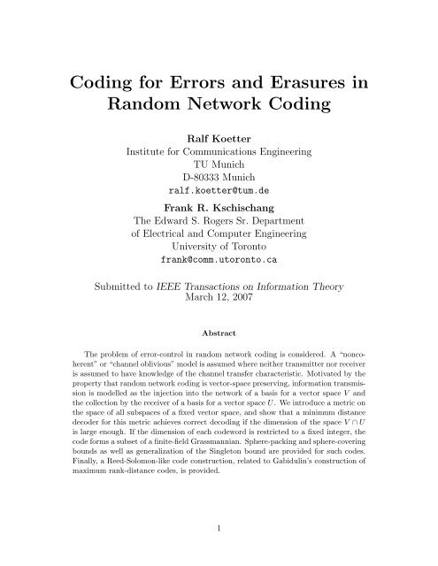
The three bounds are depicted <strong>in</strong> Fig. 1, <strong>for</strong> λ = 1/4 <strong>and</strong> <strong>in</strong> the limit as N → ∞.<br />
0.8<br />
λ=0.25<br />
0.7<br />
0.6<br />
sphere pack<strong>in</strong>g upper bound<br />
0.5<br />
code rate R<br />
0.4<br />
0.3<br />
0.2<br />
0.1<br />
sphere cover<strong>in</strong>g lower bound<br />
S<strong>in</strong>gleton upper bound<br />
0<br />
0 0.2 0.4 0.6 0.8 1 1.2 1.4 1.6 1.8 2<br />
normalized distance δ<br />
Figure 1: Upper <strong>and</strong> lower asymptotic bounds on the largest rate of a code <strong>in</strong> the Grassmann<br />
graph G W,l where the dimension N of ambient vector space is asymptotically large <strong>and</strong> λ = l N<br />
is chosen as 1/4.<br />
5. A Reed-Solomon-like Code Construction<br />
We now turn to the problem of construct<strong>in</strong>g a code capable of correct<strong>in</strong>g errors <strong>and</strong> erasures<br />
at the output of the operator channels def<strong>in</strong>ed <strong>in</strong> Section 2.<br />
15
5.1. L<strong>in</strong>earized Polynomials<br />
Let F q be a f<strong>in</strong>ite field <strong>and</strong> let F = F q m be an extension field. Recall from [20, Ch. 11], [21,<br />
Sec. 4.9], [22, Sec. 3.4] that a polynomial L(x) is called a l<strong>in</strong>earized polynomial over F if it<br />
takes the <strong>for</strong>m<br />
d∑<br />
L(x) = a i x qi , (4)<br />
i=0<br />
with coefficients a i ∈ F, i = 0, . . . , d. If all coefficients are zero, so that L(x) is the zero<br />
polynomial, we will write L(x) ≡ 0; more generally, we will write L 1 (x) ≡ L 2 (x) if L 1 (x) −<br />
L 2 (x) ≡ 0. When q is fixed under discussion, we will let x [i] denote x qi . In this notation, a<br />
l<strong>in</strong>earized polynomial over F may be written as<br />
L(x) =<br />
d∑<br />
a i x [i] .<br />
i=0<br />
The l<strong>in</strong>earized polynomial L(x) <strong>in</strong> (4) has conventional q-associate<br />
l(x) =<br />
d∑<br />
a i x i .<br />
i=0<br />
If L(x) is a l<strong>in</strong>earized polynomial, we will refer to the degree of its conventional q-associate<br />
as the associate degree of L(x). Clearly a l<strong>in</strong>earized polynomial of associate degree d has<br />
actual degree q d .<br />
If L 1 (x) <strong>and</strong> L 2 (x) are l<strong>in</strong>earized polynomials over F, then so is any F-l<strong>in</strong>ear comb<strong>in</strong>ation<br />
α 1 L 1 (x) + α 2 L 2 (x), α 1 , α 2 ∈ F . The ord<strong>in</strong>ary product L 1 (x)L 2 (x) is not necessarily a<br />
l<strong>in</strong>earized polynomial. However, the composition L 1 (L 2 (x)), often written as L 1 (x) ⊗ L 2 (x),<br />
of two l<strong>in</strong>earized polynomials over F is aga<strong>in</strong> a l<strong>in</strong>earized polynomial over F. Note that this<br />
operation is not commutative, i.e., L 1 (x) ⊗ L 2 (x) need not be equal to L 2 (x) ⊗ L 1 (x).<br />
The product L 1 (x) ⊗ L 2 (x) of l<strong>in</strong>earized polynomials is computed explicitly as follows. If<br />
L 1 (x) = ∑ i0 a ix [i] <strong>and</strong> L 2 (x) = ∑ j0 b jx [j] , then<br />
L 1 (x) ⊗ L 2 (x) = L 1 (L 2 (x) = ∑ i0<br />
a i (L 2 (x)) [i]<br />
= ∑ ( ) [i]<br />
∑<br />
a i b j x [j]<br />
i0 j0<br />
= ∑ ∑<br />
a i b [i]<br />
j x[i+j] = ∑ c k x [k]<br />
i0 j0<br />
k0<br />
where<br />
c k =<br />
k∑<br />
i=0<br />
16<br />
a i b [i]<br />
k−i .
Thus the coefficients of L 1 (x) ⊗ L 2 (x) are obta<strong>in</strong>ed from those of L 1 (x) <strong>and</strong> L 2 (x) via a<br />
modified convolution operation. If L 1 (x) has associate degree d 1 <strong>and</strong> L 2 (x) has associate<br />
degree d 2 , then both L 1 (x) ⊗ L 2 (x) <strong>and</strong> L 2 (x) ⊗ L 1 (x) have associate degree d 1 + d 2 .<br />
Under addition + <strong>and</strong> composition ⊗, the set of l<strong>in</strong>earized polynomials over F <strong>for</strong>ms a<br />
non-commutative r<strong>in</strong>g with identity. Although non-commutative, this r<strong>in</strong>g has many of<br />
the properties of a Euclidean doma<strong>in</strong> <strong>in</strong>clud<strong>in</strong>g, <strong>for</strong> example, an absence of zero-divisors.<br />
The degree (or associate degree) of a nonzero element <strong>for</strong>ms a natural norm. There are<br />
two division algorithms: a left division <strong>and</strong> a right division, i.e., given any two l<strong>in</strong>earized<br />
polynomials a(x) <strong>and</strong> b(x), it is easy to prove by <strong>in</strong>duction that there exist unique l<strong>in</strong>earized<br />
polynomials q L (x), q R (x), r L (x) <strong>and</strong> r R (x) such that<br />
a(x) = q L (x) ⊗ b(x) + r L (x) = b(x) ⊗ q R (x) + r R (x),<br />
where r L (x) ≡ 0 or deg(r L (x)) < deg(b(x)) <strong>and</strong> similarly where r R (x) ≡ 0 or deg(r R (x)) <<br />
deg(b(x)).<br />
The polynomials q R (x) <strong>and</strong> r R (x) are easily determ<strong>in</strong>ed by the follow<strong>in</strong>g straight<strong>for</strong>ward<br />
variation of ord<strong>in</strong>ary polynomial long division. Let lc(a(x)) denote the lead<strong>in</strong>g coefficient of<br />
a(x), so that if a(x) has associate degree d, i.e., a(x) = a d x [d] + a d−1 x [d−1] + · · · + a 0 x [0] with<br />
a d ≠ 0, then lc(a(x)) = a d .<br />
procedure RDiv(a(x), b(x))<br />
<strong>in</strong>put: a pair a(x), b(x) of l<strong>in</strong>earized polynomials over F = F m q , with b(x) ≢ 0.<br />
output: a pair q(x), r(x) of l<strong>in</strong>earized polynomials over F m q<br />
beg<strong>in</strong><br />
if deg(a(x)) < deg(b(x)) then<br />
return (0, a(x))<br />
else<br />
d := deg(a(x)), e := deg(b(x)), a d := lc(a(x)), b e := lc(b(x))<br />
t(x) := (a d /b e ) [m−e] x [d−e] (*)<br />
return (t(x), 0) + RDiv(a(x) − b(x) ⊗ t(x), b(x)) (**)<br />
endif<br />
end<br />
Note that the parameter m <strong>in</strong> step (*) is equal to the dimension of F m q as a vector space<br />
over F q . This algorithm term<strong>in</strong>ates when it produces polynomials q(x) <strong>and</strong> r(x) with the<br />
property that a(x) = b(x) ⊗ q(x) + r(x) <strong>and</strong> either r(x) ≡ 0 or deg r(x) < deg b(x).<br />
The left-division procedure is essentially the same; “RDiv” is replaced with “LDiv” <strong>and</strong> (*)<br />
<strong>and</strong> (**) are replaced with the follow<strong>in</strong>g:<br />
t(x) := (a d /(b [d−e]<br />
e ))x [d−e]<br />
return (t(x), 0) + LDiv(a(x) − t(x) ⊗ b(x), b(x))<br />
17
With this change, the algorithm term<strong>in</strong>ates when it produces polynomials q(x) <strong>and</strong> r(x)<br />
with the property that a(x) = q(x) ⊗ b(x) + r(x).<br />
L<strong>in</strong>earized polynomials receive their name from the follow<strong>in</strong>g property. Let L(x) be a l<strong>in</strong>earized<br />
polynomial over F, <strong>and</strong> let K be an arbitrary extension field of F. Then K may be<br />
regarded as a vector space over F q . The map tak<strong>in</strong>g β ∈ K to L(β) ∈ K is l<strong>in</strong>ear with<br />
respect to F q , i.e., <strong>for</strong> all β 1 , β 2 ∈ K <strong>and</strong> all λ 1 , λ 2 ∈ F q ,<br />
L(λ 1 β 1 + λ 2 β 2 ) = λ 1 L(β 1 ) + λ 2 L(β 2 ).<br />
Suppose that K is chosen to be large enough to <strong>in</strong>clude all the zeros of L(x). The zeros of<br />
L(x) then correspond to the kernel of L(x) regarded as a l<strong>in</strong>ear map, so they <strong>for</strong>m a vector<br />
space over F q . This vector space has dimension equal to at most the associate degree of<br />
L(x), but the dimension could possibly be smaller if L(x) has repeated roots (which occurs<br />
if <strong>and</strong> only if a 0 = 0 <strong>in</strong> (4)).<br />
On the other h<strong>and</strong> if V is an n-dimensional subspace of K, then<br />
L(x) = ∏ β∈V<br />
(x − β)<br />
is a monic l<strong>in</strong>earized polynomial over K (though not necessarily over F). See [21, Lemma<br />
21] or [22, Theorem 3.52].<br />
The follow<strong>in</strong>g lemma shows that if two l<strong>in</strong>earized polynomials of degree at most d − 1 agree<br />
on at least d l<strong>in</strong>early <strong>in</strong>dependent po<strong>in</strong>ts, then the two polynomials co<strong>in</strong>cide.<br />
Lemma 12 Let d be a positive <strong>in</strong>teger <strong>and</strong> let f(x) <strong>and</strong> g(x) be two l<strong>in</strong>earized polynomials<br />
over F of associate degree less than d. If α 1 , α 2 , . . . , α d are l<strong>in</strong>early <strong>in</strong>dependent elements of<br />
K such that have f(α i ) = g(α i ) <strong>for</strong> i = 1, . . . , d, then f(x) ≡ g(x).<br />
Proof. Observe that h(x) = f(x) − g(x) has α 1 , . . . , α d as zeros, <strong>and</strong> hence also has all<br />
q d l<strong>in</strong>ear comb<strong>in</strong>ations of these elements as zeros. Thus h(x) has at least q d dist<strong>in</strong>ct zeros.<br />
However, s<strong>in</strong>ce the actual degree of h(x) is strictly smaller than q d , this is only possible if<br />
h(x) ≡ 0.<br />
5.2. Code Construction<br />
Just as traditional Reed-Solomon codeword components may be obta<strong>in</strong>ed via the evaluation<br />
of an ord<strong>in</strong>ary message polynomial, we obta<strong>in</strong> here a basis <strong>for</strong> the transmitted vector space<br />
via the evaluation of a l<strong>in</strong>earized message polynomial.<br />
Let F q be a f<strong>in</strong>ite field, <strong>and</strong> let F = F q m be a (f<strong>in</strong>ite) extension field of F q . As <strong>in</strong> the<br />
previous subsection, we may regard F as a vector space of dimension m over F q . Let A =<br />
18
{α 1 , . . . , α l } ⊂ F be a set of l<strong>in</strong>early <strong>in</strong>dependent elements <strong>in</strong> this vector space. These<br />
elements span an l-dimensional vector space 〈A〉 ⊆ F over F q . Clearly l m. We will take<br />
as ambient space the direct sum W = 〈A〉 ⊕ F = {(α, β) : α ∈ 〈A〉, β ∈ F}, a vector space of<br />
dimension l + m over F q .<br />
Let u = (u 0 , u 1 , . . . , u k−1 ) ∈ F k denote a block of message symbols, consist<strong>in</strong>g of k symbols<br />
over F or, equivalently, mk symbols over F q . Let F k [x] denote the set of l<strong>in</strong>earized polynomials<br />
over F of associate degree at most k − 1. Let f(x) ∈ F k [x], def<strong>in</strong>ed as<br />
∑k−1<br />
f(x) = u i x [i] ,<br />
i=0<br />
be the l<strong>in</strong>earized polynomial with coefficients correspond<strong>in</strong>g to u. F<strong>in</strong>ally, let β i = f(α i ).<br />
Each pair (α i , β i ), i = 1, . . . , l, may be regarded as a vector <strong>in</strong> W . S<strong>in</strong>ce {α 1 , . . . , α l } is a<br />
l<strong>in</strong>early <strong>in</strong>dependent set, so is {(α 1 , β 1 ), . . . , (α l , β l )}; hence this set spans an l-dimensional<br />
subspace V of W . We denote the map that takes the message polynomial f(x) ∈ F k [x] to<br />
the l<strong>in</strong>ear space V ∈ P(W, |A|) as ev A .<br />
Lemma 13 If |A| k then the map ev A : F k [x] → P(W, |A|) is <strong>in</strong>jective.<br />
Proof. Suppose |A| k <strong>and</strong> ev A (f) = ev A (g) <strong>for</strong> some f(x), g(x) ∈ F k [x]. Let h(x) =<br />
f(x) − g(x). Clearly h(α i ) = 0 <strong>for</strong> i = 1, . . . , l. S<strong>in</strong>ce h(x) is a l<strong>in</strong>earized polynomial, it<br />
follows that h(x) = 0 <strong>for</strong> all x ∈ 〈A〉. Thus h(x) has at least q |A| q k zeros, which is only<br />
possible (s<strong>in</strong>ce h(x) has associate degree at most k − 1) if h(x) ≡ 0, so that f(x) ≡ g(x).<br />
Hence<strong>for</strong>th we will assume that l k. Lemma 13 implies that, provided this condition<br />
is satisfied, the image of F k [x] is a code C ⊆ P(W, l) with q mk codewords. The m<strong>in</strong>imum<br />
distance of C is given by the follow<strong>in</strong>g theorem; however, first we need the follow<strong>in</strong>g lemma.<br />
Lemma 14 If {(α 1 , β 1 ), . . . , (α r , β r )} ⊆ W is a collection of r l<strong>in</strong>early <strong>in</strong>dependent elements<br />
satisfy<strong>in</strong>g β i = f(α i ) <strong>for</strong> some l<strong>in</strong>earized polynomial f over F, then {α 1 , . . . , α r } is a l<strong>in</strong>early<br />
<strong>in</strong>dependent set.<br />
Proof. Suppose that <strong>for</strong> some γ 1 , . . . , γ r ∈ F q we have ∑ r<br />
i=1 γ iα i = 0. Then, <strong>in</strong> W , we<br />
would have<br />
(<br />
r∑<br />
r∑<br />
) (<br />
) ( (<br />
r∑<br />
r∑<br />
r∑<br />
))<br />
γ i (α i , β i ) = γ i α i , γ i β i = 0, γ i f(α i ) = 0, f γ i α i<br />
i=1<br />
i=1 i=1<br />
i=1<br />
i=1<br />
= (0, f(0)) = (0, 0),<br />
which is possible (s<strong>in</strong>ce the (α i , β i ) pairs are l<strong>in</strong>early <strong>in</strong>dependent) only if γ 1 , . . . , γ r = 0.<br />
Theorem 15 Let C be the image under ev A of F k [x], with l = |A| k. Then C is a code of<br />
type [l + m, l, mk, 2(l − k + 1)].<br />
19
Proof. Only the m<strong>in</strong>imum distance is <strong>in</strong> question. Let f(x) <strong>and</strong> g(x) be dist<strong>in</strong>ct elements<br />
of F k [x], <strong>and</strong> let U = ev A (f) <strong>and</strong> V = ev A (g). Suppose that U ∩ V has dimension r. This<br />
means it is possible to f<strong>in</strong>d r l<strong>in</strong>early <strong>in</strong>dependent elements (α ′ 1, β ′ 1), . . . , (α ′ r, β ′ r) such that<br />
f(α ′ i) = g(α ′ i) = β ′ i, i = 1, . . . , r. By Lemma 14, α ′ 1, . . . , α ′ r are l<strong>in</strong>early <strong>in</strong>dependent <strong>and</strong><br />
hence they span an r-dimensional space B with the property that f(b) = g(b) = 0 <strong>for</strong> all<br />
b ∈ B. If r k then f(x) <strong>and</strong> g(x) would be two l<strong>in</strong>earized polynomials of associate degree<br />
less than k that agree on at least k l<strong>in</strong>early <strong>in</strong>dependent po<strong>in</strong>ts, <strong>and</strong> hence by Lemma 12,<br />
we would have f(x) ≡ g(x). S<strong>in</strong>ce this is not the case, we must have r k − 1. Thus<br />
d(U, V ) = dim(U) + dim(V ) − 2 dim(U ∩ V ) = 2(l − r) 2(l − k + 1).<br />
It is easy to exhibit two codewords U <strong>and</strong> V that satisfy this bound with equality.<br />
The S<strong>in</strong>gleton bound, evaluated <strong>for</strong> the code parameters of Theorem 15, states that<br />
[ ] [ ]<br />
N − (D − 2)/2 m + k<br />
|C| <br />
= < 4q mk .<br />
l − (D − 2)/2 k<br />
This implies that a true S<strong>in</strong>gleton-bound-achiev<strong>in</strong>g code could have no more than 4 times<br />
as many codewords as C. When N is large enough, the difference <strong>in</strong> rate between C <strong>and</strong> a<br />
S<strong>in</strong>gleton-bound-achiev<strong>in</strong>g becomes negligible. Indeed, <strong>in</strong> terms of normalized parameters,<br />
we have<br />
R = (1 − λ)(1 − δ + 1<br />
λN )<br />
which certa<strong>in</strong>ly has the same asymptotic behavior as the S<strong>in</strong>gleton bound <strong>in</strong> the limit as<br />
N → ∞. We claim, there<strong>for</strong>e, that these Reed-Solomon-like codes are nearly S<strong>in</strong>gletonbound-achiev<strong>in</strong>g.<br />
We note also that the traditional network code C of Example 1, a code of type [m+l, l, ml, 2],<br />
is obta<strong>in</strong>ed as a special case of these codes by sett<strong>in</strong>g k = l.<br />
This code construction <strong>in</strong>volv<strong>in</strong>g the evaluation of l<strong>in</strong>earized polynomials is clearly closely<br />
related to the rank-metric code construction of Gabidul<strong>in</strong> [11]. However, <strong>in</strong> our setup, the<br />
codewords are not arrays, but rather the vector spaces spanned by the rows of the array, <strong>and</strong><br />
the relevant decod<strong>in</strong>g metric is not the rank metric, but rather the distance measure def<strong>in</strong>ed<br />
<strong>in</strong> (2).<br />
q<br />
q<br />
5.3. Decod<strong>in</strong>g<br />
Suppose now that V ∈ C is transmitted over the operator channel described <strong>in</strong> Section 2 <strong>and</strong><br />
that an (l − ρ + t)-dimensional subspace U of W is received, where dim(U ∩ V ) = l − ρ. In<br />
this situation, we have ρ erasures <strong>and</strong> an error norm of t, <strong>and</strong> d(U, V ) = ρ + t. We expect to<br />
be able to recover V from U provided that ρ + t < D/2 = l − k + 1, <strong>and</strong> we will describe a<br />
Sudan-style “list-1” m<strong>in</strong>imum distance decod<strong>in</strong>g algorithm to do so (see, e.g., [23, Sec. 9.3]).<br />
Note that, even if t = 0, we require ρ < l − k + 1, or l − ρ k, i.e., not surpris<strong>in</strong>gly (given<br />
20
that we are attempt<strong>in</strong>g to recover mk <strong>in</strong><strong>for</strong>mation symbols), the receiver must collect enough<br />
vectors to span a space of dimension at least k.<br />
Let r = l−ρ+t denote the dimension of the received space U, <strong>and</strong> let (x i , y i ), i = 1, . . . , r be<br />
a basis <strong>for</strong> U. At the decoder we suppose that it is possible to construct a nonzero bivariate<br />
polynomial Q(x, y) of the <strong>for</strong>m<br />
Q(x, y) = Q x (x) + Q y (y), such that Q(x i , y i ) = 0 <strong>for</strong> i = 1, . . . , r, (5)<br />
where Q x (x) is a l<strong>in</strong>earized polynomial over F q m of associate degree at most τ − 1 <strong>and</strong> Q y (y)<br />
is a l<strong>in</strong>earized polynomial over F q m of associate degree at most τ − k. Although Q(x, y) is<br />
chosen to <strong>in</strong>terpolate only a basis <strong>for</strong> U, s<strong>in</strong>ce Q(x, y) is a l<strong>in</strong>earized polynomial, it follows<br />
that <strong>in</strong> fact Q(x, y) = 0 <strong>for</strong> all (x, y) ∈ U.<br />
We note that (5) def<strong>in</strong>es a homogeneous system of r equations <strong>in</strong> 2τ − k + 1 unknown<br />
coefficients. This system has a nonzero solution when it is under-determ<strong>in</strong>ed, i.e., when<br />
r = l − ρ + t < 2τ − k + 1. (6)<br />
S<strong>in</strong>ce f(x) is a l<strong>in</strong>earized polynomial over F q m, so is Q(x, f(x)), given by<br />
Q(x, f(x)) = Q x (x) + Q y (f(x)) = Q x (x) + Q y (x) ⊗ f(x).<br />
S<strong>in</strong>ce the associate degree of f(x) is at most k − 1, the associate degree of Q(x, f(x)) is at<br />
most τ − 1.<br />
Now let {(a 1 , b 1 ), . . . , (a l−ρ , b l−ρ )} be a basis <strong>for</strong> U ∩ V . S<strong>in</strong>ce all vectors of U are zeros of<br />
Q(x, y), we have Q(a i , b i ) = 0 <strong>for</strong> i = 1, . . . , l − ρ. However, s<strong>in</strong>ce (a i , b i ) ∈ V we also have<br />
b i = f(a i ) <strong>for</strong> i = 1, . . . , l − ρ. In particular,<br />
Q(a i , b i ) = Q(a i , f(a i )) = 0, i = 1, . . . , l − ρ,<br />
thus Q(x, f(x)) is a l<strong>in</strong>earized polynomial hav<strong>in</strong>g a 1 , . . . , a l−ρ as roots. By Lemma 14, these<br />
roots are l<strong>in</strong>early <strong>in</strong>dependent. Thus Q(x, f(x)) is a l<strong>in</strong>earized polynomial of associate degree<br />
at most τ that evaluates to zero on a space of dimension l − ρ. If the condition<br />
l − ρ τ (7)<br />
holds, then Q(x, f(x)) has more zeros than its degree, which is only possible if Q(x, f(x)) ≡ 0.<br />
S<strong>in</strong>ce <strong>in</strong> general<br />
Q(x, y) = Q y (y − f(x)) + Q(x, f(x)),<br />
we have, when Q(x, f(x)) ≡ 0,<br />
Q(x, y) = Q y (y − f(x))<br />
<strong>and</strong> so we may hope to extract y − f(x) from Q(x, y). Equivalently, we may hope to f<strong>in</strong>d<br />
f(x) from the equation<br />
Q y (x) ⊗ f(x) + Q x (x) ≡ 0. (8)<br />
21
However, this equation is easily solved us<strong>in</strong>g the RDiv procedure described <strong>in</strong> Section 5.1,<br />
with a(x) = −Q x (x) <strong>and</strong> b(x) = Q y (x). Alternatively, we can exp<strong>and</strong> (8) <strong>in</strong>to a system of<br />
equations <strong>in</strong>volv<strong>in</strong>g the unknown coefficients of f(x); this system is readily solved recursively<br />
(i.e., via back-substitution).<br />
In summary, to f<strong>in</strong>d nonzero Q(x, y) we must satisfy (6) <strong>and</strong> to ensure that Q(x, f(x)) ≡ 0<br />
we must satisfy (7). When both (6) <strong>and</strong> (7) hold <strong>for</strong> some τ, we say that the received space<br />
U is decodable.<br />
Suppose that the received space U is decodable. Substitut<strong>in</strong>g (7) <strong>in</strong>to (6), we obta<strong>in</strong> the<br />
condition l − ρ + t < 2(l − ρ) − k + 1 or, equivalently,<br />
i.e., not surpris<strong>in</strong>gly decodability implies (9).<br />
ρ + t < l − k + 1, (9)<br />
Conversely, suppose (9) is satisfied. From (9) we get l − ρ t + k, or<br />
By select<strong>in</strong>g<br />
l − ρ + t + k = r + k 2(l − ρ). (10)<br />
τ = ⌈ r + k<br />
2 ⌉<br />
(which is possible to do s<strong>in</strong>ce the receiver knows both r <strong>and</strong> k), we satisfy (6). With this<br />
choice of τ, <strong>and</strong> apply<strong>in</strong>g condition (10), we see that<br />
τ l − ρ + 1/2;<br />
however, s<strong>in</strong>ce l, ρ <strong>and</strong> τ are <strong>in</strong>tegers, we see that (7) is also satisfied. In other words,<br />
condition (9) implies decodability, which is precisely what we would have hoped <strong>for</strong>.<br />
The <strong>in</strong>terpolation polynomial Q(x, y) can be obta<strong>in</strong>ed from the r basis vectors (x 1 , y 1 ),<br />
(x 2 , y 2 ), . . . , (x r , y r ) <strong>for</strong> U via any method that provides a nonzero solution to the homogeneous<br />
system (5). We next describe an efficient algorithm to accomplish this task.<br />
Let f(x, y) = f x (x)+f y (y) be a bivariate l<strong>in</strong>earized polynomial which means that both f x (x)<br />
<strong>and</strong> f y (y) are l<strong>in</strong>earized polynomials. Let the associate degree of f x (x) <strong>and</strong> f y (y) be d x (f)<br />
<strong>and</strong> d y (f), respectively. The (1, k − 1)-weighted degree of f(x, y) is def<strong>in</strong>ed as<br />
deg 1,k−1 (f(x, y)) := max{d x (f), k − 1 + d y (f)}<br />
Note that this def<strong>in</strong>ition is different from the weighted degree def<strong>in</strong>itions <strong>for</strong> usual bivariate<br />
polynomials. However, it should become more natural by observ<strong>in</strong>g that we may write f(x, y)<br />
as f(x, y) = f x (x) + f y (x) ⊗ y.<br />
The follow<strong>in</strong>g adaptation of an algorithm <strong>for</strong> the <strong>in</strong>terpolation problem <strong>in</strong> Sudan-type decod<strong>in</strong>g<br />
algorithms (see e.g. [24, 25]) provides an efficient way to f<strong>in</strong>d the required bivariate<br />
l<strong>in</strong>earized polynomial Q(x, y). Let a vector space U be spanned by r l<strong>in</strong>early <strong>in</strong>dependent<br />
po<strong>in</strong>ts (x i , y i ) ∈ W .<br />
22
procedure Interpolate(U)<br />
<strong>in</strong>put: a basis (x i , y i ) ∈ W , i = 1, . . . , r, <strong>for</strong> U<br />
output: a l<strong>in</strong>earized bivariate polynomial Q(x, y) = Q x (x) + Q y (y)<br />
<strong>in</strong>itialization: f 0 (x, y) = x, f 1 (x, y) = y<br />
beg<strong>in</strong><br />
<strong>for</strong> i = 1 to r do<br />
∆ 0 := f 0 (x i , y i ); ∆ 1 := f 1 (x i , y i )<br />
if ∆ 0 = 0 then<br />
f 1 (x, y) := f q 1 (x, y) − ∆ q−1<br />
1 f 1 (x, y)<br />
elseif ∆ 1 = 0 then<br />
f 0 (x, y) := f q 0 (x, y) − ∆ q−1<br />
0 f 0 (x, y)<br />
else<br />
if deg 1,k−1 (f 0 ) deg 1,k−1 (f 1 ) then<br />
f 1 (x, y) := ∆ 1 f 0 (x, y) − ∆ 0 f 1 (x, y)<br />
f 0 (x, y) := f q 0 (x, y) − ∆ q−1<br />
0 f 0 (x, y)<br />
else<br />
f 0 (x, y) := ∆ 1 f 0 (x, y) − ∆ 0 f 1 (x, y)<br />
f 1 (x, y) := f q 1 (x, y) − ∆ q−1<br />
1 f 1 (x, y)<br />
endif<br />
end<strong>for</strong><br />
if deg 1,k−1 (f 1 ) < deg 1,k−1 (f 0 ) then<br />
return f 0 (x, y)<br />
else<br />
return f 1 (x, y)<br />
endif<br />
end<br />
For completeness we provide a proof of correctness of this algorithm, which mimics the proof<br />
<strong>in</strong> the case of st<strong>and</strong>ard bivariate <strong>in</strong>terpolation, f<strong>in</strong>d<strong>in</strong>g the ideal of polynomials that vanishes<br />
at a given set of po<strong>in</strong>ts [24, 25].<br />
Def<strong>in</strong>e an order ≺ on bivariate l<strong>in</strong>earized polynomials as follows: write f(x, y) ≺ g(x, y)<br />
if deg 1,k−1 (f(x, y)) < deg 1,k−1 (g(x, y)). In case deg 1,k−1 (f(x, y)) = deg 1,k−1 (g(x, y)) write<br />
f(x, y) ≺ g(x, y) if d y (f) + k − 1 < deg 1,k−1 (f(x, y)) <strong>and</strong> d y (g) + k − 1 = deg 1,k−1 (g(x, y)). If<br />
none of these conditions is true, we say that f(x, y) <strong>and</strong> g(x, y) are not comparable. While ≺<br />
is clearly not a total order on polynomials, it is granular enough <strong>for</strong> the proof of correctness<br />
of procedure Interpolate. In particular, ≺ gives a total order on monomials <strong>and</strong> we can,<br />
hence, def<strong>in</strong>e a lead<strong>in</strong>g term lt ≺ (f) as the maximal monomial (without its coefficient) <strong>in</strong> f<br />
under the order ≺.<br />
Lemma 16 Assume that we have two bivariate l<strong>in</strong>earized polynomials f(x, y) <strong>and</strong> g(x, y)<br />
which are not comparable under ≺. We can create a l<strong>in</strong>ear comb<strong>in</strong>ation h(x, y) = f(x, y) +<br />
γg(x, y) which <strong>for</strong> a suitably chosen γ yields a polynomial h(x, y) with h(x, y) ≺ f(x, y) <strong>and</strong><br />
h(x, y) ≺ g(x, y).<br />
23
Proof. If f(x, y) <strong>and</strong> g(x, y) are not comparable then we have lt ≺ (f) = lt ≺ (g). Choos<strong>in</strong>g<br />
γ as the quotient of the correspond<strong>in</strong>g coefficients of lt ≺ (f) <strong>in</strong> f <strong>and</strong> lt ≺ (g) <strong>in</strong> g yields a<br />
polynomial h(x, y) such that lt ≺ (h) ≺ lt ≺ (f) = lt ≺ (g).<br />
Let A be a set of r l<strong>in</strong>early <strong>in</strong>dependent po<strong>in</strong>ts (x i , y i ) ∈ W . We say that a nonzero polynomial<br />
f(x, y) is x-m<strong>in</strong>imal with respect to A if f(x, y) is a m<strong>in</strong>imal polynomial under ≺ such<br />
that lt ≺ (f) = x [dx(f)] <strong>and</strong> f(x, y) vanishes at all po<strong>in</strong>ts of A. Similarly, a nonzero polynomial<br />
g(x, y) is said to be y-m<strong>in</strong>imal with respect to A if g(x, y) is a a m<strong>in</strong>imal polynomial under<br />
≺ such that lt ≺ (g) = y [dy(g)] <strong>and</strong> g(x, y) vanishes <strong>in</strong> all po<strong>in</strong>ts of A.<br />
Theorem 17 The polynomials f 0 (x, y) <strong>and</strong> f 1 (x, y) that are output by procedure Interpolate<br />
are x-m<strong>in</strong>imal <strong>and</strong> y-m<strong>in</strong>imal with respect to the given set of r l<strong>in</strong>early <strong>in</strong>dependent po<strong>in</strong>ts<br />
(x i , y i ) ∈ W .<br />
Proof. First we note that x-m<strong>in</strong>imal <strong>and</strong> y-m<strong>in</strong>imal polynomials can always be compared<br />
under ≺ s<strong>in</strong>ce they have different lead<strong>in</strong>g monomials. The proof proceeds by <strong>in</strong>duction.<br />
We first verify that the polynomials x <strong>and</strong> y are x-m<strong>in</strong>imal <strong>and</strong> y-m<strong>in</strong>imal with respect to<br />
the empty set. We thus assume that after j iterations of the <strong>in</strong>terpolation algorithm the<br />
polynomials f 0 (x, y) <strong>and</strong> f 1 (x, y) are x-m<strong>in</strong>imal <strong>and</strong> y-m<strong>in</strong>imal with respect to the po<strong>in</strong>ts<br />
(x i , y i ), i = 1, 2, . . . , j. It is easy to check that the set of polynomials constructed <strong>in</strong> the<br />
next iteration also vanishes at the po<strong>in</strong>t (x j+1 , y j+1 ) so this part of the def<strong>in</strong>ition of x- <strong>and</strong><br />
y-m<strong>in</strong>imality with respect to po<strong>in</strong>ts (x i , y i ), i = 1, 2, . . . , j + 1 will not be a problem.<br />
Assume first the generic case that ∆ 0 ≠ 0 <strong>and</strong> ∆ 1 ≠ 0. Assume that f 1 (x, y) ≺ f 0 (x, y)<br />
holds. Let f 0(x, ′ y) = ∆ 1 f 0 (x, y) − ∆ 0 f 1 (x, y). In this case lt ≺ (f 0(x, ′ y)) = lt ≺ (f 0 (x, y))<br />
<strong>and</strong> the x-m<strong>in</strong>imality of f 0(x, ′ y) follows from the x-m<strong>in</strong>imality of f 0 (x, y). Let f 1(x, ′ y) =<br />
f q 1 (x, y)−∆ q−1<br />
1 f 1 (x, y). We will show that f 1(x, ′ y) is y-m<strong>in</strong>imal with respect to po<strong>in</strong>ts (x i , y i ),<br />
i = 1, 2, . . . , j + 1. To this end <strong>and</strong> <strong>in</strong> order to arrive at a contradiction assume that f 1(x, ′ y)<br />
is not y-m<strong>in</strong>imal. This would imply that there exists a y-m<strong>in</strong>imal polynomial f 1 ′′ (x, y) w.r.t.<br />
po<strong>in</strong>ts (x i , y i ), i = 1, 2, . . . , j + 1 such that f 1 ′′ (x, y) ≠ f 1 (x, y) which has the same lead<strong>in</strong>g<br />
term as f 1 (x, y). The two polynomials are clearly different s<strong>in</strong>ce f 1 ′′ (x, y) would vanish at<br />
(x j+1 , y j+1 ) while f 1 (x, y) does not. But this would imply that we can f<strong>in</strong>d a polynomial<br />
h(x, y) as l<strong>in</strong>ear comb<strong>in</strong>ation of f 1 ′′ (x, y) <strong>and</strong> f 1 (x, y) which would precede both f 0 (x, y) <strong>and</strong><br />
f 1 (x, y) under the order ≺ <strong>and</strong> which would vanish at all po<strong>in</strong>ts (x i , y i ), i = 1, 2, . . . , j + 1,<br />
thus contradict<strong>in</strong>g the m<strong>in</strong>imality of f 0 (x, y) <strong>and</strong> f 1 (x, y). A virtually identical arguments<br />
holds if we have f 0 (x, y) ≺ f 1 (x, y).<br />
Next we consider the case that ∆ 0 equals 0 while we have ∆ 1 ≠ 0. In this case f 0 (x, y) is<br />
unchanged <strong>and</strong>, hence, <strong>in</strong>herits its x-m<strong>in</strong>imality from the previous iteration. We only have<br />
to check that the newly constructed f 1(x, ′ y) = f q 1 (x, y) − ∆ q−1<br />
1 f 1 (x, y) is y-m<strong>in</strong>imal with<br />
respect to po<strong>in</strong>ts (x i , y i ), i = 1, 2, . . . , j + 1. Aga<strong>in</strong>, assum<strong>in</strong>g the opposite would imply that<br />
there exists a polynomial f 1 ′′ (x, y) ≠ f 1 (x, y) with the same lead<strong>in</strong>g term as f 1 (x, y). The<br />
two polynomials are aga<strong>in</strong> different s<strong>in</strong>ce f 1 ′′ (x, y) would vanish at (x j+1 , y j+1 ) while f 1 (x, y)<br />
does not. Aga<strong>in</strong>, we <strong>for</strong>m a suitable l<strong>in</strong>ear comb<strong>in</strong>ation h(x, y) of f 1 ′′ (x, y) <strong>and</strong> f 1 (x, y)<br />
which would precede f 1 (x, y) under ≺. If the lead<strong>in</strong>g term of h(x, y) is of type y [dy(h)] or<br />
24
h(x, y) ≺ f 0 (x, y) we have arrived at a contradiction negat<strong>in</strong>g the y-m<strong>in</strong>imality of f 1 (x, y)<br />
or the x-m<strong>in</strong>imality of f 0 (x, y). Otherwise, note that h(x, y) does not vanish at (x j+1 , y j+1 )<br />
<strong>and</strong> hence is not a multiple (under ⊗ of f 0 (x, y).) Hence, <strong>for</strong> a suitably chosen t, we can f<strong>in</strong>d<br />
a polynomial h ′′ (x, y) as a l<strong>in</strong>ear comb<strong>in</strong>ation of h(x, y) <strong>and</strong> x [t] ⊗ f 0 (x, y) which precedes<br />
h(x, y). Repeat<strong>in</strong>g this procedure we arrive at a polynomial ĥ(x, y) which either has a lead<strong>in</strong>g<br />
term of type y [dy(ĥ)] or which precedes f 0 (x, y) under ≺, either contradict<strong>in</strong>g the y-m<strong>in</strong>imality<br />
of f 1 (x, y) or the x-m<strong>in</strong>imality of f 0 (x, y). F<strong>in</strong>ally we note that the case ∆ 0 ≠ 0 <strong>and</strong> ∆ 1 = 0<br />
follows from similar arguments. For the case ∆ 0 = 0 <strong>and</strong> ∆ 1 = 0 there is noth<strong>in</strong>g to prove.<br />
Based on Theorem 17 we can claim that the Interpolate procedure solves the problem—as<br />
required <strong>in</strong> equation (5)—of f<strong>in</strong>d<strong>in</strong>g the bivariate l<strong>in</strong>earized polynomial Q(x, y) of m<strong>in</strong>imal<br />
(1, k − 1) weighted degree τ − 1, which is identified as the polynomial f 0 (x, y) or f 1 (x, y) of<br />
smaller (1, k − 1) weighted degree.<br />
Let V ∈ C be transmitted over the operator channel described <strong>in</strong> Section 2 <strong>and</strong> assume that<br />
an (l − ρ + t)-dimensional subspace U of W is received. Decod<strong>in</strong>g comprises the follow<strong>in</strong>g<br />
steps:<br />
1. Invoke Interpolate(U) to f<strong>in</strong>d a bivariate l<strong>in</strong>earized polynomial Q(x, y) = Q x (x) +<br />
Q y (y) of m<strong>in</strong>imal (1, k − 1) weighted degree that vanishes on the vector space U.<br />
2. Invoke RDiv(−Q x (x), Q y (x)) to f<strong>in</strong>d a l<strong>in</strong>earized polynomial f(x) with the property<br />
that −Q x (x) ≡ Q y (x) ⊗ f(x). If no such polynomial can be found declare “failure.”<br />
3. Output f(x) as the <strong>in</strong><strong>for</strong>mation polynomial correspond<strong>in</strong>g the codeword V ∈ C if<br />
d(U, V ) < l − k + 1.<br />
6. Conclusions<br />
In this paper we have def<strong>in</strong>ed a class of operator channels as the natural transmission models<br />
<strong>in</strong> “noncoherent” r<strong>and</strong>om network cod<strong>in</strong>g. The <strong>in</strong>puts <strong>and</strong> outputs of operator channels are<br />
subspaces of some given ambient vector space. We have def<strong>in</strong>ed a cod<strong>in</strong>g metric on these<br />
subspaces which gives rise to notions of erasures (dimension reduction) <strong>and</strong> errors (dimension<br />
enlargement). In def<strong>in</strong><strong>in</strong>g codes, it is natural to restrict each codeword to have some fixed<br />
dimension; <strong>in</strong> this case, the code <strong>for</strong>ms a subset of a f<strong>in</strong>ite-field Grassmannian. Spherepack<strong>in</strong>g<br />
<strong>and</strong> sphere-cover<strong>in</strong>g bounds as well as a S<strong>in</strong>gleton-type bound are obta<strong>in</strong>ed <strong>in</strong> this<br />
context. F<strong>in</strong>ally, a Reed-Solomon-like code construction is given, result<strong>in</strong>g <strong>in</strong> codes that are<br />
capable of correct<strong>in</strong>g various comb<strong>in</strong>ations of errors <strong>and</strong> erasures.<br />
Acknowledgment<br />
The authors thank Danilo Silva <strong>for</strong> useful discussions.<br />
25
References<br />
[1] T. Ho, R. Koetter, M. Médard, D. Karger, <strong>and</strong> M. Effros, “The benefits of cod<strong>in</strong>g over<br />
rout<strong>in</strong>g <strong>in</strong> a r<strong>and</strong>omized sett<strong>in</strong>g,” <strong>in</strong> Proc. 2003 IEEE Int. Symp. on In<strong>for</strong>m. Theory,<br />
(Yokohama), p. 442, June 29 – July 4, 2003.<br />
[2] P. A. Chou, Y. Wu, <strong>and</strong> K. Ja<strong>in</strong>, “Practical network cod<strong>in</strong>g,” <strong>in</strong> Proc. 2003 Allerton<br />
Conf. on Commun., Control <strong>and</strong> Comput<strong>in</strong>g, (Monticello, IL), Oct. 2003.<br />
[3] T. Ho, M. Médard, R. Koetter, D. Karger, M. Effros, J. Shi, <strong>and</strong> B. Leong, “A r<strong>and</strong>om<br />
l<strong>in</strong>ear network cod<strong>in</strong>g approach to multicast,” IEEE Trans. on In<strong>for</strong>m. Theory, vol. 52,<br />
pp. 4413–4430, Oct. 2006.<br />
[4] L. Zheng <strong>and</strong> D. N. C. Tse, “Communication on the Grassmannian manifold: A geometric<br />
approach to the noncoherent multiple-antenna channel,” IEEE Trans. on In<strong>for</strong>m.<br />
Theory, vol. 48, pp. 359–383, Feb. 2002.<br />
[5] N. Cai <strong>and</strong> R. W. Yeung, “<strong>Network</strong> cod<strong>in</strong>g <strong>and</strong> error correction,” <strong>in</strong> Proc. 2002 IEEE<br />
In<strong>for</strong>m. Theory Workshop, pp. 119–122, Oct. 20–25, 2002.<br />
[6] L. Song, R. W. Yeung, <strong>and</strong> N. Cai, “Zero-error network cod<strong>in</strong>g <strong>for</strong> acyclic networks,”<br />
IEEE Trans. on In<strong>for</strong>m. Theory, vol. 49, pp. 3129–3139, Dec. 2003.<br />
[7] R. W. Yeung <strong>and</strong> N. Cai, “<strong>Network</strong> error correction, part I: Basic concepts <strong>and</strong> upper<br />
bounds,” Comm. <strong>in</strong> In<strong>for</strong>m. <strong>and</strong> Systems, vol. 6, no. 1, pp. 19–36, 2006.<br />
[8] R. W. Yeung <strong>and</strong> N. Cai, “<strong>Network</strong> error correction, part II: Lower bounds,” Comm.<br />
<strong>in</strong> In<strong>for</strong>m. <strong>and</strong> Systems, vol. 6, no. 1, pp. 37–54, 2006.<br />
[9] Z. Zhang, “<strong>Network</strong> error correction cod<strong>in</strong>g <strong>in</strong> packetized networks,” <strong>in</strong> Proc. 2006 IEEE<br />
In<strong>for</strong>m. Theory Workshop, Oct. 22–26, 2006.<br />
[10] S. Jaggi, M. Langberg, S. Katti, T. Ho, D. Katabi, <strong>and</strong> M. Médard, “Resilient network<br />
cod<strong>in</strong>g <strong>in</strong> the presence of Byzant<strong>in</strong>e adversaries,” <strong>in</strong> Proc. 26th Annual IEEE Conf. on<br />
Computer Commun., INFOCOM, (Anchorage, AK), May 6–12, 2007. (To appear.).<br />
[11] E. M. Gabidul<strong>in</strong>, “Theory of codes with maximal rank distance,” Problems of In<strong>for</strong>mation<br />
Transmission, vol. 21, pp. 1–12, July 1985.<br />
[12] D. Silva <strong>and</strong> F. R. Kschischang, “Us<strong>in</strong>g rank-metric codes <strong>for</strong> error correction <strong>in</strong> r<strong>and</strong>om<br />
network cod<strong>in</strong>g.” (Submitted to the 2007 IEEE International Symposium on In<strong>for</strong>mation<br />
Theory.), 2007.<br />
[13] P. V. Ceccher<strong>in</strong>i, “A q-analogous of the characterization of hypercubes as graphs,” J.<br />
of Geometry, vol. 22, pp. 57–74, 1984.<br />
[14] A. E. Brouwer, A. M. Cohen, <strong>and</strong> A. Neumaier, Distance-Regular Graphs. New York,<br />
NY: Spr<strong>in</strong>ger Verlag, 1989.<br />
26
[15] L. Chihara, “On the zeros of the Askey-Wilson polynomials, with applications to cod<strong>in</strong>g<br />
theory,” SIAM J. Math. Anal., vol. 18, no. 1, pp. 191–207, 1987.<br />
[16] W. J. Mart<strong>in</strong> <strong>and</strong> X. J. Zhu, “Anticodes <strong>for</strong> the Grassmann <strong>and</strong> bil<strong>in</strong>ear <strong>for</strong>ms graphs,”<br />
Designs, Codes <strong>and</strong> Cryptography, vol. 6, pp. 73–79, 1995.<br />
[17] R. Ahlswede, H. K. Ayd<strong>in</strong>ian, <strong>and</strong> L. H. Khachatrian, “On perfect codes <strong>and</strong> related<br />
concepts,” Designs, Codes <strong>and</strong> Cryptography, vol. 22, pp. 221–237, 2001.<br />
[18] M. Schwartz <strong>and</strong> T. Etzion, “Codes <strong>and</strong> anticodes <strong>in</strong> the Grassmann graph,” J. of<br />
Comb<strong>in</strong>. Theory Series A, vol. 97, pp. 27–42, 2002.<br />
[19] J. H. van L<strong>in</strong>t <strong>and</strong> R. M. Wilson, A Course <strong>in</strong> Comb<strong>in</strong>atorics. Cambridge, UK: Cambridge<br />
University Press, second ed., 2001.<br />
[20] E. R. Berlekamp, Algebraic <strong>Cod<strong>in</strong>g</strong> Theory. New York: McGraw-Hill, 1968.<br />
[21] F. J. MacWilliams <strong>and</strong> N. J. A. Sloane, The Theory of Error-Correct<strong>in</strong>g Codes. New<br />
York: North Holl<strong>and</strong>, 1977.<br />
[22] R. Lidl <strong>and</strong> H. Niederreiter, F<strong>in</strong>ite Fields. Read<strong>in</strong>g, MA: Addison-Wesley, 1983. Vol. 20<br />
of The Encyclopedia of Mathematics, G.-C. Rota, Ed.<br />
[23] R. M. Roth, Introduction to <strong>Cod<strong>in</strong>g</strong> Theory. Cambridge, UK: Cambridge University<br />
Press, 2006.<br />
[24] R. J. McEliece, “The Guruswami-Sudan decod<strong>in</strong>g algorithm <strong>for</strong> Reed-Solomon codes,”<br />
tech. rep., JPL Interplanetary <strong>Network</strong> Progress Report 42-153, 2003. Available onl<strong>in</strong>e<br />
at www.systems.caltech.edu/EE/Faculty/rjm/papers/RSD-JPL.pdf.<br />
[25] R. J. McEliece, B. Wang, <strong>and</strong> K. Watanabe, “Koetter <strong>in</strong>terpolation over modules,” <strong>in</strong><br />
Proc. 2005 Allerton Conf. on Commun., Control <strong>and</strong> Comput<strong>in</strong>g, (Monticello, IL), Oct.<br />
2005.<br />
27


