Mechanics - 3B Scientific
Mechanics - 3B Scientific
Mechanics - 3B Scientific

Create successful ePaper yourself
Turn your PDF publications into a flip-book with our unique Google optimized e-Paper software.
UE105060<br />
<strong>3B</strong> SCIENTIFIC® PHYSICS EXPERIMENT<br />
For the motions ϕ + = ϕ1 + ϕ2<br />
and ϕ − = ϕ1 − ϕ2<br />
(initially<br />
chosen arbitrarily) the equation of motion is as follows:<br />
L ⋅ ϕ&&<br />
L ⋅ ϕ&&<br />
+<br />
−<br />
+ g ⋅ ϕ<br />
+<br />
+<br />
The solutions<br />
ϕ<br />
ϕ<br />
+<br />
−<br />
= 0<br />
( g + 2k) ⋅ ϕ = 0<br />
= a cos<br />
+<br />
= a cos<br />
−<br />
−<br />
( ω+<br />
t) + b+<br />
sin( ω+<br />
t)<br />
( ω t) + b sin( ω t)<br />
−<br />
give rise to angular frequencies<br />
−<br />
−<br />
g<br />
g + 2k<br />
ω + = und ω − =<br />
(4)<br />
L<br />
L<br />
corresponding to the natural frequencies for in phase or out<br />
of phase motion (ϕ +<br />
= 0 for out of phase motion and ϕ –<br />
= 0<br />
for in-phase motion).<br />
The deflection of the pendulums can be calculated from the<br />
sum or the difference of the two motions, leading to the<br />
solutions<br />
1<br />
ϕ1<br />
=<br />
2<br />
1<br />
ϕ2<br />
=<br />
2<br />
( a cos( ω t) + b sin( ω t) + a cos( ω t) + b sin( ω t)<br />
)<br />
+<br />
( a cos( ω t) + b sin( ω t) − a cos( ω t) − b sin( ω t)<br />
)<br />
+<br />
+<br />
+<br />
+<br />
+<br />
+<br />
+<br />
Parameters a +<br />
, a –<br />
, b +<br />
and b –<br />
are arbitrary coefficients that<br />
can be calculated from the initial conditions for the two<br />
pendulums at time t = 0.<br />
The easiest case to interpret is where pendulum 1 is deflected<br />
by an angle ϕ 0 from its rest position and released at<br />
time 0 while pendulum 2 remains in its rest position.<br />
1<br />
ϕ1<br />
= ⋅<br />
2<br />
1<br />
ϕ2<br />
= ⋅<br />
2<br />
( ϕ ⋅ cos( ω t) + ϕ ⋅cos( ω t)<br />
)<br />
0<br />
+<br />
( ϕ ⋅ cos( ω t) − ϕ ⋅ cos( ω t)<br />
)<br />
0<br />
+<br />
0<br />
After rearranging the equations they take the form<br />
ϕ1<br />
= ϕ0<br />
⋅ cos<br />
ϕ = ϕ ⋅ sin<br />
2<br />
with<br />
0<br />
ω−<br />
− ω<br />
ω∆<br />
=<br />
2<br />
ω+<br />
+ ω−<br />
ω =<br />
2<br />
0<br />
( ω∆t) ⋅cos( ωt)<br />
( ω t) ⋅cos( ωt)<br />
+<br />
∆<br />
This corresponds to an oscillation of both pendulums at<br />
identical angular frequency ω, where the amplitudes are<br />
modulated at an angular frequency ω ∆ . This kind of modulation<br />
results in beats. In the situation described, the amplitude<br />
of the beats arrives at a maximum since the overall<br />
amplitude falls to a minimum at zero.<br />
−<br />
−<br />
−<br />
−<br />
−<br />
−<br />
−<br />
−<br />
−<br />
−<br />
(2)<br />
(3)<br />
(5)<br />
(6)<br />
(7)<br />
(8)<br />
LIST OF APPARATUS<br />
2 Pendulum rods with angle sensor U8404270<br />
1 Transformer 12 V, 2 A, e.g. U8475430<br />
1 Helical spring with two eyelets, 3 N/m U15027<br />
2 Table clamps U13260<br />
2 Stainless steel rods, 1000 mm U15004<br />
1 Stainless steel rod, 470 mm U15002<br />
4 Universal clamps U13255<br />
1 <strong>3B</strong> NETlog U11300<br />
1 <strong>3B</strong> NETlab for Windows U11310<br />
1 PC with Windows 98/2000/XP, Internet Explorer 6 or later,<br />
USB port<br />
SET-UP<br />
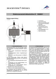
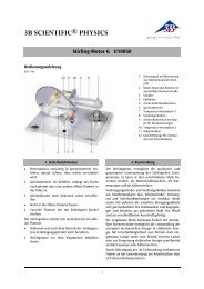
Fig. 2<br />
Set-up for recording and evaluating the oscillation of two<br />
identical pendulums coupled together by a spring<br />
The set-up is illustrated in Fig. 2.<br />
• Clamp two stand rods of 1000 mm length to a bench so<br />
that they are about 15 cm apart.<br />
• Attach a short stand rod between them as a horizontal<br />
cross member to lend the set-up more stability.<br />
• Attach the angle sensors to the top of the vertical rods<br />
using universal clamps.<br />
• Attach bobs to the end of the pendulum rods.<br />
• Suspend the pendulum rods from the angle sensors<br />
(there are grooves in the angle sensors to accommodate<br />
the hinge pins of the pendulum rods)<br />
2 / 5