poster - International Conference of Agricultural Engineering

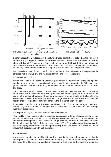
z
5 cm
-10 cm
-20 cm
5
4
3
Pressure
head
Volumetric
water content
m
0.0
-0.4
-0.8
-1.2
-1.6
0.25
0.15
-10cm -20cm -30cm
-30 cm
2
1
Tensiometer
Soil moisture
probe
Thermometer
FIGURE 1: Schematic illustration of observation
and computation
Soil
temperature
0.05
o
C
20
10
0
11/26 11/27 11/28 11/29 11/30 12/1 12/2
Time in day
FIGURE 2: Observed data
Eq.(10), respectively. Additionally, the saturated water content θ s is defined as the value of θ
in case that ψ is equal to zero while the residual water content θ r as the minimum value in
observed data of θ. Thus, θ s and θ r are determined to be 0.30 and 0.05 from all observed
data series including them shown in Fig.2, respectively. As the reference soil temperature,
the average value of observed data is adopted which equals to 12.4 degrees Celsius.
Conclusively, a best fitting curve for θ −ψ relation at the reference soil temperature is
obtained with the value of α and n vg being 28.9 m -1 and 1.43, respectively.
4.3 Identification of RHC
Firstly, the number of identified unknown parameters is determined. Since the optimal
number of parameters is approximately from seven to nine according to Bitterlich et al.
(2004) and Iden and Durner (2007), the number of unknown parameters is set to be 10 in
this study.
Secondly, the manner of division on the definition domain (effective saturation domain) is
determined. The function shape of RHC generally has steeper gradient near the saturated
zone. In the context of accuracy, the range with steeper gradient should be divided into finer
subdomain. Therefore the effective saturation range from 0.8 to 1.0 where RHC function
rapidly changes is partitioned into sub-range in the manner of geometric series.
Eventually, RHC function is identified as shown in Fig.3 after the saturated hydraulic
conductivity at the reference temperature is determined to be 5.18×10 -5 m/s through
laboratory experiment.
4.4 Reproducibility of Calibrated Forward Simulation Model
The validity of the inverse modeling proposed is assessed in terms of reproducibility for the
time-series observed data by calibrated forward simulation model through comparing the
observed and computed values. The result of reproducibility for water movement is shown in
Fig.4. In the lower half of Fig.4, the absolute errors |ψ obs -ψ com | are also shown to demonstrate
the time-varying difference in solution reproducibility. From the results, it is found that water
movement is reproduced with high accuracy.
5. Conclusion
An inverse modeling in variably saturated and non-isothermal subsurface water flow is
developed. To consider the water movement depending on the soil temperature, a couple of
the mixed form RE with heat conduction equation is employed as the governing equation.