Chapter 2 Some functions and their derivatives
Chapter 2 Some functions and their derivatives
Chapter 2 Some functions and their derivatives

You also want an ePaper? Increase the reach of your titles
YUMPU automatically turns print PDFs into web optimized ePapers that Google loves.
<strong>Chapter</strong> 2<br />
<strong>Some</strong> <strong>functions</strong> <strong>and</strong> <strong>their</strong> <strong>derivatives</strong><br />
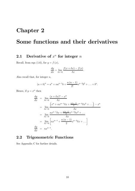
2.1 Derivative of x n for integer n<br />
Recall, from eqn (1.6), for y = f (x),<br />
Also recall that, for integer n,<br />
Hence, if y = x n then<br />
dy<br />
dx = lim<br />
δx→0<br />
(a + b) n = a n + na n−1 b +<br />
f(x + δx) ¡ f(x)<br />
.<br />
δx<br />
n (n ¡ 1)<br />
a n−2 b 2 + ...+ b n .<br />
2!<br />
dy<br />
dx = lim (x + δx) n ¡ x n<br />
δx→0<br />
³<br />
δx<br />
´<br />
x n + nx n−1 δx + n(n−1) x n−2 δx 2 + ...<br />
2<br />
= lim<br />
δx→0 δx<br />
nx n−1 δx + n(n−1) x n−2 δx 2 + ...<br />
2<br />
= lim<br />
δx→0<br />
·<br />
= lim nx n−1 +<br />
δx→0<br />
dy<br />
dx = nxn−1 .<br />
2.2 Trigonometric Functions<br />
See Appendix C for further details.<br />
δx<br />
n (n ¡ 1)<br />
x n−2 δx + ...<br />
2<br />
¸<br />
¡ x n<br />
10
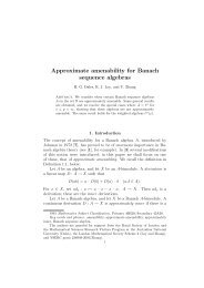
2.2.1 Definition <strong>and</strong> Graphs of Sine <strong>and</strong> Cosine<br />
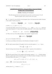
The two basic trigonometric <strong>functions</strong> are the sine <strong>and</strong> cosine. Fromanangleθ, we<br />
may define cos θ <strong>and</strong> sin θ geometrically. Given the point P in the (x, y) plane such that<br />
OP is of length 1 <strong>and</strong> makes an anticlockwise angle θ with the positive x axis, then<br />
cos θ = x-coordinate of P.<br />
sin θ = y-coordinate of P.<br />
In the figure, 0 < θ < π 2<br />
<strong>and</strong>, for the right-angled triangle OAP,<br />
sin θ =<br />
length of side opposite to θ<br />
length of hypotenuse<br />
, cos θ =<br />
length of side adjactent to θ<br />
.<br />
length of hypotenuse<br />
In calculus, <strong>and</strong> THROUGHOUT THIS COURSE, all angles will be measured<br />
in RADIANS. In the picture, the angle θ inradiansisdefined to be the length of the<br />
arc from the point (1, 0) to P of the circle of radius 1 centre O.<br />
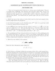
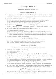
Our geometrical definitions of cos θ <strong>and</strong> sin θ make sense not just for 0 < θ < π/2 as<br />
in the picture but for all real values of θ of either sign. The graphs of these two <strong>functions</strong><br />
in the range (¡3π, 3π) are:<br />
11
By considering the limiting cases of the previously illustrated right-angled triangle<br />
when θ =0<strong>and</strong> when θ = π/2, we immediately deduce (in accordance with the graphs<br />
just drawn) that<br />
2.2.2 Inverse Trigonometric Functions<br />
sin 0 = 0, (2.1)<br />
cos π 2<br />
= 0, (2.2)<br />
cos 0 = 1, (2.3)<br />
sin π 2<br />
= 1. (2.4)<br />
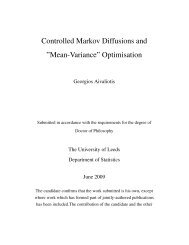
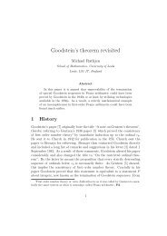
From the form of the graph of the sine function, we see that it cannot have an inverse<br />
as it st<strong>and</strong>s, since each horizontal line y = c (with ¡1
sin : £ ¡ π 2 , π 2<br />
¤<br />
! [¡1, 1] has increasing inverse sin −1 =arcsin:[¡1, 1] ! £ ¡ π 2 , π 2<br />
¤<br />
. By<br />
definition, given any y in [¡1, 1], sin −1 y istheuniqueanglebetween¡π/2 <strong>and</strong> π/2 whose<br />
sine is y.<br />
NB. It is totally different from (sin y) −1 =cosec y.<br />
NB The graph of sin −1 y has vertical tangents at y = §1, sotheslope dx<br />
dy<br />
these two points.<br />
is infinite at<br />
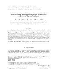
Question: Over what restriction will cos have an inverse, arccos?<br />
Answer: We restrict cos to be either increasing or decreasing. It is usual to choose the<br />
decreasing restriction cos : [0, π] ! [¡1, 1], with inverse arccos : [¡1, 1] ! [0, π].<br />
13
As for arcsin,givenanyy in [¡1, 1], cos −1 (y) = arccos y istheuniqueanglebetween0 <strong>and</strong> π<br />
whose cosine is y.<br />
tan <strong>and</strong> arctan<br />
14
The function tan is increasing over many intervals, but we conventionally take the interval<br />
containing x =0: tan : (¡π/2, π/2) ! R with inverse arctan : R ! (¡π/2, π/2).<br />
15
2.2.3 <strong>Some</strong> identities <strong>and</strong> a useful limit<br />
NB.AnidentityisanequationwhichholdsforALLpermittedvaluesofitsvariables.<br />
See Appendix C for proofs of many trig. identities. Three which will be used in the next<br />
section are<br />
sin(x + y) = sinx cos y +cosx sin y, (2.5)<br />
cos 2x = 1¡ 2sin 2 x (2.6)<br />
cos 2 x +sin 2 x = 1. (2.7)<br />
Appendix C4 also contains the proof of a useful limit:<br />
sin x<br />
lim =1,<br />
x→0 x<br />
(2.8)<br />
i.e. sin x ¼ x for small angles x.<br />
2.2.4 Derivatives of the trigonometric <strong>functions</strong><br />
By definition (see section 1.4), the derivative of sin x is<br />
d<br />
(sin x) = lim<br />
dx δx→0<br />
sin(x + δx) ¡ sin x<br />
δx<br />
sin x cos δx +cosx sin δx ¡ sin x<br />
= lim<br />
δx→0 δx<br />
sin x (cos δx ¡ 1) + cos x sin δx<br />
= lim<br />
δx→0 δx<br />
¡2sinx sin 2 (δx/2) + cos x sin δx<br />
= lim<br />
δx→0 δx<br />
·sin δx/2<br />
δx<br />
= ¡ sin x lim<br />
δx→0 2 δx/2<br />
= cosx using (2.8).<br />
¸2<br />
+cosx lim<br />
δx→0<br />
sin δx<br />
δx<br />
using (2.5)<br />
using (2.6)<br />
This is eqn B.4 of Appendix B. There is a similar proof that<br />
d<br />
(cos x) =¡ sin x.<br />
dx<br />
Derivatives of other trig <strong>functions</strong> may be derived from those of sin <strong>and</strong> cos. e.g,<br />
using the quotient rule:<br />
µ <br />
d<br />
d sin x<br />
(tan x) =<br />
dx dx cos x<br />
cos x (cos x) ¡ sin x(¡ sin x)<br />
=<br />
cos 2 x<br />
= cos2 x +sin 2 x<br />
cos 2 x<br />
1<br />
=<br />
using (2.7)<br />
cos 2 x<br />
= sec 2 x.<br />
One similarly deduces that<br />
d<br />
dx (cot x) =¡cosec2 x.<br />
The remaining <strong>derivatives</strong> are all given in Appendix B.<br />
16
2.2.5 Derivatives of the inverse trigonometric <strong>functions</strong><br />
Derivatives of inverse <strong>functions</strong> To find the <strong>derivatives</strong> of inverse <strong>functions</strong>, we use<br />
the result<br />
dy<br />
dx = ³<br />
1 ´ , provided dx<br />
dx<br />
dy 6=0<br />
which follows directly from the definition of the derivative.<br />
dy<br />
Inverse Sine Set y =sin −1 x <strong>and</strong> x =siny (with ¡π/2 · y · π/2 <strong>and</strong> ¡1
Repeatedly differentiating (2.9), we see that<br />
d 2 y<br />
dx = dy<br />
2 dx = y, <strong>and</strong> more generally dn y<br />
= y for all positive integers n.<br />
dxn It follows (from Taylor’s Theorem - which you haven’t met yet!) that a function satisfies<br />
condition (2.9) if <strong>and</strong> only if<br />
y(x) =y(0)<br />
·1+x ¢¢¢¸<br />
+ x2<br />
2! + x3<br />
3! + = y(0)<br />
∞X<br />
n=0<br />
x n<br />
n!<br />
for all real x, (2.10)<br />
where n! =n(n ¡ 1)(n ¡ 2) ...3.2.1 is the product of the first n positive integers (called<br />
“factorial n”) <strong>and</strong> y(0) is the value of y(x) at x =0.<br />
For now, you can satisfy yourself that (2.10) “works” by differentiating it:<br />
dy<br />
dx = y(0) d<br />
dx<br />
·<br />
= y(0)<br />
= y(0)<br />
·1+x + x2<br />
2! + x3<br />
3! + ¢¢¢¸<br />
¸<br />
¢¢¢<br />
0+1+ 2x<br />
2! + 3x2 + 4x3<br />
3! 4!<br />
·1+x ¢¢¢¸<br />
+ x2<br />
2! + x3<br />
3! + = y(x).<br />
It turns out that the sum of infinitely many terms is nevertheless finite in value for any<br />
real x. [It is an example of a Taylor series, ofwhichmorelateroninthis course.]<br />
Definition of the exponential function We define the exponential function exp(x)<br />
to be the unique function (defined for all real x) satisfying the two conditions<br />
d<br />
[exp(x)]<br />
dx<br />
= exp(x) (for all real x), (2.11)<br />
exp (0) = 1. (2.12)<br />
Theuniquefunctionexp(x) satisfying these is given explicitly by<br />
This definition:<br />
exp(x) =1+x + x2<br />
2! + x3<br />
3! + ¢¢¢= ∞<br />
X<br />
n=0<br />
x n<br />
n! . (2.13)<br />
² allows the numerical evaluation of exp (x) for all real x.<br />
² allows one to show (see Appendix D.1) that:<br />
exp (x + y) = exp(x)exp(y) ,<br />
exp (x) > 0,<br />
exp (¡x) =<br />
1<br />
exp (x)<br />
Given exp (x) > 0 it follows from (2.11) that d [exp(x)] > 0 <strong>and</strong> so<br />
dx<br />
exp (x) is a strictly increasing function, i.e. x>y) exp(x) > exp(y). (2.14)<br />
18
From 2.13 we can see that<br />
<strong>and</strong> so, given exp (¡x) = 1<br />
exp(x) ,<br />
So, the graph of the function exp(x) looks like:<br />
exp(x) ! +1 as x ! +1, (2.15)<br />
exp(x) ! 0 as x !¡1. (2.16)<br />
2.3.2 The Logarithmic Function<br />
Since exp : R ! (0, 1) is a strictly increasing function, it must have a (unique) strictly<br />
increasing inverse ln : (0, 1) ! R called the logarithmic function or natural logarithm.<br />
For x 2 R, y2 (0, 1),<br />
y =exp(x) if <strong>and</strong> only if x =lny. (2.17)<br />
Taking x =0in (2.17) <strong>and</strong> using exp (0) = 1, weseethat<br />
Similarly it follows from (2.15), (2.16) <strong>and</strong> (2.17) that<br />
ln 1 = 0. (2.18)<br />
ln x ! +1 as x ! +1, (2.19)<br />
ln x ! ¡1 as x ! 0. (2.20)<br />
Properties (2.18)—(2.20) all show up clearly on the graph of ln:<br />
19
2.3.3 Definition of an Arbitrary Real Power of a Positive Real<br />
Number<br />
We know<br />
so we see<br />
exp(x 1 + x 2 )=exp(x 1 )exp(x 2 ) (2.21)<br />
exp(x 1 + x 2 + ¢¢¢+ x n )=exp(x 1 )exp(x 2 ) ...exp(x n ), (2.22)<br />
where n is any positive integer <strong>and</strong> x 1 ,x 2 ,...,x n any real numbers. Taking x 1 = x 2 =<br />
¢¢¢= x n =lnx, wherex>0, <strong>and</strong> using (2.17), we get<br />
exp(n ln x) =[exp(lnx)] n = x n ,<br />
for any positive integer n.<br />
We can define an arbitrary real power x α of a positive real number x by<br />
equivalent [by (2.17)] to<br />
x α =exp(α ln x) (x>0, α real), (2.23)<br />
ln(x α )=α ln x (x >0, α real). (2.24)<br />
The definition (2.23) satisfies the st<strong>and</strong>ard rules for multiplication <strong>and</strong> division of<br />
powers:<br />
for all real α <strong>and</strong> β.<br />
x α x β = x α+β ,<br />
x α<br />
x β = x α−β ,<br />
20
2.3.4 The Number e, <strong>and</strong> the Exponential Function as a Power<br />
We define the positive real number e (whose value is approximately 2.718) by<br />
e =exp1, (2.25)<br />
from which<br />
Using (2.23),<br />
i.e.<br />
2.3.5 Derivatives<br />
The exponential function<br />
ln e =1. (2.26)<br />
e x =exp(x ln e) =exp(x)<br />
exp x = e x for all real x. (2.27)<br />
By definition.<br />
d<br />
[exp(x)] = exp(x). (2.28)<br />
dx<br />
The logarithmic function<br />
y =lnx, <strong>and</strong>sox =exp(y) . Then<br />
d<br />
dx [ln(x)] = 1 dx<br />
dy<br />
=<br />
1<br />
exp (y) = 1 x<br />
(for x>0). (2.29)<br />
Arbitrary real powers<br />
From the above definition of x α we have<br />
d<br />
dx (xα ) = d (exp (α ln x))<br />
dx<br />
= exp(α ln x)£ α £ 1 x<br />
(using the chain rule)<br />
= αx α 1 x<br />
= αx α−1 .<br />
Thus<br />
d<br />
dx (xα )=αx α−1 (α real, x>0), (2.30)<br />
NBthereisasimilartrickfor<br />
d<br />
dx (ax )= d (exp (x ln a)) = ...<br />
dx<br />
2.4 The Hyperbolic Functions<br />
These are constructed from the exponential function, but obey identities closely analogous<br />
to those satisfied by the corresponding trigonometric <strong>functions</strong> (obtained by dropping the<br />
final “h”).<br />
21
2.4.1 Definitions<br />
cosh x = 1 2 (ex + e −x ), (2.31)<br />
sinh x = 1 2 (ex ¡ e −x ), (2.32)<br />
tanh x = sinh x<br />
cosh x = ex ¡ e −x 1 ¡ e−2x<br />
=<br />
e x + e−x 1+e = e2x ¡ 1<br />
−2x e 2x +1 , (2.33)<br />
coth x = 1<br />
tanh x = cosh x<br />
sinh x = ex + e −x 1+e−2x<br />
=<br />
e x ¡ e−x 1 ¡ e = e2x +1<br />
−2x e 2x ¡ 1<br />
(x 6= 0),(2.34)<br />
sech x = 1<br />
cosh x = 2<br />
,<br />
e x + e−x (2.35)<br />
cosech x = 1<br />
sinh x = 2<br />
e x ¡ e −x (x 6= 0). (2.36)<br />
2.4.2 The Fundamental Identity<br />
Corresponding to the well-known identity cos 2 x +sin 2 x =1for the trigonometric <strong>functions</strong>,<br />
we have for the hyperbolic <strong>functions</strong> the identity<br />
cosh 2 x ¡ sinh 2 x =1 (2.37)<br />
(holding for all real x). NB the minus sign! To prove (2.37), just substitute the definitions<br />
(2.31) <strong>and</strong> (2.32) into the LHS, to get<br />
1<br />
4 (ex +e −x ) 2 ¡ 1 4 (ex ¡e −x ) 2 = 1 4 (e2x +e −2x +2e x e −x )¡ 1 4 (e2x +e −2x ¡2e x e −x )=e x e −x = e x−x = e 0 =1.<br />
2.4.3 Further Identities<br />
1 ¡ tanh 2 x = sech 2 x, (2.38)<br />
coth 2 x ¡ 1 = cosech 2 x, (2.39)<br />
sinh(x + y) = sinhx cosh y +coshx sinh y, (2.40)<br />
sinh(x ¡ y) = sinhx cosh y ¡ cosh x sinh y, (2.41)<br />
cosh(x + y) = coshx cosh y +sinhx sinh y, (2.42)<br />
cosh(x ¡ y) = coshx cosh y ¡ sinh x sinh y, (2.43)<br />
sinh 2x = 2sinhx cosh x, (2.44)<br />
cosh 2x = sinh 2 x +cosh 2 x, (2.45)<br />
cosh 2 x = 1 (cosh 2x +1),<br />
2<br />
(2.46)<br />
sinh 2 x = 1 (cosh 2x ¡ 1),<br />
2<br />
(2.47)<br />
sinh x cosh y = 1 [sinh (x + y)+sinh(x ¡ y)] ,<br />
2<br />
(2.48)<br />
cosh x cosh y = 1 [cosh (x + y)+cosh(x ¡ y)] ,<br />
2<br />
(2.49)<br />
sinh x sinh y = 1 [cosh (x + y) ¡ cosh (x ¡ y)] .<br />
2<br />
(2.50)<br />
22
Each of these has a trigonometric counterpart (see Appendix C), but there are some<br />
important differences of sign, which should be carefully noted. The identities are all easy<br />
to prove from the definitions above.<br />
2.4.4 The Graphs of cosh, sinh <strong>and</strong> tanh<br />
Using the definitions of the hyperbolic <strong>functions</strong>, <strong>and</strong> our knowledge of the exponential<br />
function, we can sketch the following graphs <strong>and</strong> deduce some properties for the<br />
hyperbolic <strong>functions</strong>.<br />
cosh 0 = 1,<br />
cosh x ! +1 as x !§1,<br />
cosh (¡x) = cosh(x) (i.e. it is an EVEN function).<br />
23
sinh 0 = 0,<br />
sinh x ! +1 as x ! +1,<br />
sinh x ! ¡1 as x !¡1,<br />
sinh (¡x) = ¡ sinh (x) (i.e. it is an ODD function).<br />
24
tanh 0 = 0,<br />
tanh x ! +1 as x ! +1,<br />
tanh x ! ¡1 as x !¡1,<br />
tanh (¡x) = ¡ tanh (x) (i.e. it is an ODD function).<br />
Like all even <strong>functions</strong>, cosh has a a graph which is symmetrical about Oy, i.e. invariant<br />
under reflection in Oy. It has a minimum value of 1 at x =0, where its derivative<br />
sinh x is zero. On the other h<strong>and</strong>, the graphs of the <strong>functions</strong> sinh <strong>and</strong> tanh, like those of<br />
all odd <strong>functions</strong>, are invariant under rotation through 180 ◦ about O. Notethatsinh<strong>and</strong><br />
tanh are both increasing <strong>functions</strong> <strong>and</strong> that the graph of tanh has horizontal asymptotes<br />
y = §1 approached as x !§1respectively.<br />
2.4.5 Symmetry <strong>and</strong> Asymptotic Properties of other hyperbolic<br />
<strong>functions</strong><br />
Similarly, we can deduce the following properties of coth, sech <strong>and</strong> cosech:<br />
coth(¡x) =¡ coth x, sech (¡x) =sechx, cosech (¡x) =¡cosechx.<br />
coth x ! 1 as x ! +1, coth x !¡1 as x !¡1,<br />
coth x ! +1 as x ! 0 from above , coth x !¡1as x ! 0, from below,<br />
sech x ! 0 as x !§1,<br />
cosech x ! 0 as x !§1,<br />
sech 0=1<br />
cosech x ! +1 as x ! 0 from above, cosech x !¡1as x ! 0 from below.<br />
2.4.6 Inverse Hyperbolic Functions<br />
cosh<br />
We restrict cosh x to the interval [0, 1), on which it is an increasing function with<br />
increasing inverse cosh −1 :[1, 1) ! [0, 1). Fory ¸ 0, x¸ 1, wehavey =cosh −1 x ,<br />
x =coshy. cosh −1 x may be expressed in terms of logarithms as follows.<br />
If y =cosh −1 x (x ¸ 1) then y is the positive solution of the equation x =coshy,<br />
that is<br />
x = 1 ¡<br />
e y + e −y¢ .<br />
2<br />
Multiplying through by 2e y gives<br />
a quadratic for e y ,withroots<br />
2xe y = e 2y +1<br />
e 2y ¡ 2xe y +1 = 0<br />
(e y ) 2 ¡ 2xe y +1 = 0<br />
e y = 2x § p 4x 2 ¡ 4<br />
= x § p x<br />
2<br />
2 ¡ 1.<br />
³<br />
so, y = ln x § p ´<br />
x 2 ¡ 1 .<br />
25
But we want y>0, so we choose the + sign, i.e.<br />
³<br />
y =cosh −1 x =ln x + p ´<br />
x 2 ¡ 1<br />
for x ¸ 1. (2.51)<br />
sinh<br />
sinh: R ! R is an increasing function, so there is no need for restriction. By similar<br />
arguments to those used for cosh, one shows that, for any x,<br />
sinh −1 x =ln<br />
³x + p ´<br />
1+x 2 . (2.52)<br />
tanh<br />
tanh : R ! (¡1, 1) is an increasing function, so there is no need for restriction. It is easy<br />
to show that<br />
tanh −1 x = 1 µ 1+x<br />
2 ln for ¡ 1
Inverse Cosh Recall y =cosh −1 x , x =coshy with y ¸ 0, x¸ 1. So,sinh y ¸ 0<br />
<strong>and</strong> hence<br />
Then<br />
i.e.<br />
sinh 2 y = cosh 2 y ¡ 1<br />
q<br />
sinh y = + cosh 2 y ¡ 1=+ p x 2 ¡ 1.<br />
dy<br />
dx = 1 dx<br />
dy<br />
d<br />
dx (cosh−1 x)=<br />
= 1<br />
sinh y =+ 1<br />
p<br />
x2 ¡ 1<br />
1<br />
p for x>1.<br />
x2 ¡ 1<br />
You can also prove this by differentiating eqn (2.51) directly.<br />
Inverse Sinh<br />
Similarly<br />
d<br />
dx (sinh−1 x)=<br />
1<br />
p<br />
1+x<br />
2 .<br />
Inverse Tanh<br />
y =tanh −1 x ) x =tanhy, sowehave<br />
so<br />
dx<br />
dy = sech2 x =1¡ tanh 2 x =1¡ y 2 ,<br />
d<br />
dx (tanh−1 x)= 1 dx<br />
dy<br />
= 1 for ¡ 1