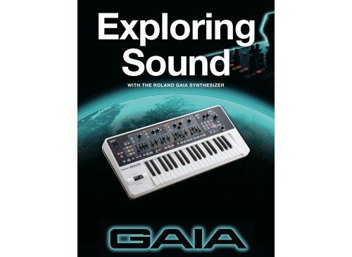
GAIA Exploring Sound (PDF) - Roland Corporation Australia

Exploring
Sound
WITH THE ROLAND GAIA SYNTHESIZER

Foreword

Welcome to the exciting world of sound, in particular, musical
sound. In this iBook you are invited to take a lesson based
approach to discover just what sound is. That may seem strange
at first. We all know what sound is, right? We hear sounds
everyday, and we’re very well adapted at recognizing them. We
find it easy to distinguish the sound of a passing train from that of
a kitten’s purr.
Taking that idea a little further, as musicians we can very easily
hear the differences between the drums and the guitars. The
string section and the brass section. Many of us may also be able
to listen to a full orchestra and recognize the oboe part. The flute.
The trumpet. Perhaps we can even discern the subtle differences
between a violin and a viola, but why? Why are they different?
allow you to prove much of the science of sound along the way.
However, although we are focusing on the GAIA, and its software,
the principles apply to many other devices. The ideas revolve
around what is known as Subtractive Synthesis, so if you have
any Subtractive Synthesizer (or software) these lessons will still
apply.
Perhaps now you have many questions. What is a digital
instrument? What was an analog synthesizer? Why do different
instruments sound so different?
The answers to all these questions will appear in the lessons to
follow. There is no need to jump ahead just yet. Our plan is to
guide you step by step. So settle back and enjoy the ride.
Certainly the differences of size and shape may provide clues, but
why can we still hear those differences with our eyes closed?
There must be a science behind all this that can explain what we
hear, and that is what we hope to explore in this text.
In this course we take advantage of a fascinating musical
instrument that is also great fun to use. It is the Roland GAIA
synthesizer. It is a modern digital instrument that can faithfully
recreate all the sounds of its analog predecessors from the 1970s
and 1980s.
We will take advantage of its Editing Software. This will not only
add to the fun by using all the power of your computer, it will also
ii

Lesson 1
An Overview
This first lesson is designed to help you get
acquainted with the GAIA and its software. You will
learn some very basic terms and have some fun
along the way.

Section 1
Terminology
Before we begin we will need to become familiar with a few
common terms.
Figure 1.1 Roland System700 (Circa 1976)
The GAIA and the Software
For example, throughout this course we will take advantage of all
the power of both the GAIA synthesizer, and its Synthesizer
Sound Designer software on your computer. You see? Even
saying it that way makes it sound more difficult than it needs to
be. From now on let’s refer to the instrument as simply “the
GAIA”, and the combination of computer and Designer Software
as “the software.”
A Patch
Another term; Patch. In the early days synthesizers looked very
different to what you see in the GAIA before you. They were
rarely an “all-in-one” product. They usually consisted of a
collection of boxes that were connected by cables.
These cables were called “patch cables”. You may recall the
phone operator in an old movie saying; “I’ll patch you through.”
As a result, it became common practice to refer to the resulting
combination of synthesizer pieces as a “patch.”
Because this is an iBook you can use standard Apple tap and pinch
gestures to zoom an image. You can also return to the table of
contents by “pinching” an entire page.
4

Now take a look at the GAIA. You can see that it has several very
clearly marked sections.
Figure 1.2 Roland GAIA Synthesizer
You can immediately see a familiar word; Patch. This is where you
can begin to have some fun, and experience some of the sonic
power of the GAIA.
For the next five minutes we’d like you to try the patches. Start by
selecting the PRESET PATCH button. Now select one of the
NUMBER buttons, and play the keyboard.
At first it appears that there are 8 Preset Patches, but there really
are 64! Can you find the others? That’s right. The Bank button.
You can access the 8 Banks by holding the Bank button and
selecting from the Number buttons. 8 Banks by 8 Patches. Please
experiment.
We only need to concentrate on one section for now. In fact, in
later chapters you will realize that the GAIA is even simpler to
understand than what it appears to be in this picture.
Let’s begin with the area just above the middle of the keyboard,
as shown in Figure 1.3.
Figure 1.3 The Patch Selectors
Before the five minutes are up, please try the first 8 Preset
Patches again.
Is it possible to play chords with all of them?
Would you say they are all musical sounds?
Could you give them a name? A description?
For further information about Patches in the GAIA please refer to
page 18 of the GAIA Owner’s Manual; Selecting Sounds
5

TONE versus Tone
Throughout this book we have to rely upon some common terms.
Unfortunately, in synthesis a few terms can convey a variety of
meanings. One of those is the word; tone.
You have heard people refer to the “tone” of a person’s voice, the
“tonal character” of an oboe, etc.. However, in synthesis we often
use the word “tone” to describe one small part of a sound. In fact,
with the GAIA we really have three synthesizers combined into
one, and refer to them as the “three TONES”.
There is a very simple way to describe the character or brightness
of the sound. We can use the words Tone Color.
So, throughout this book we will use the following definitions for
clarity:
TONE, one of the three synthesizers in the GAIA.
Tone Color, the character of the sound.
Take a look at Figure 1.4, which displays an area to the left side of
the GAIA. It confirms that the GAIA includes three TONES.
Figure 1.4 The TONE Selectors
How are we to distinguish between these two meanings of the
word?
6

Section 2
The Initial Patch
To Initialize the Patch
This is a small step, but very important. An Initial Patch on the
GAIA is a powerful starting point. It not only creates a very basic
sound, it also simplifies our explanation by allowing us to always
start from the same place.
To initialize a patch from the software is very easy, but for now
we’ll just use the GAIA. On the GAIA it is not quite so obvious,
but really very simple. Take a look at Figure 1.5, you will see a
CANCEL/SHIFT button, and a WRITE button.
Figure 1.5 Shift & Write
Try it. It is a very raw sound that can be quite musical, but more
importantly it is a great starting point that we will use throughout
this book. That is, we will often ask you to:
Initialize the Patch
To help you remember this procedure please think of the SHIFT/
WRITE process as a special form of writing a Patch. Just
pressing WRITE will save the Patch to memory, but SHIFT/
WRITE creates a whole new (Initialized) patch.
In the software you can find a dedicated Initialize button that
achieves the same result. Knowing both methods can be useful, and
you may wish to choose your favorite.
In this case we’ll think of the first as just the SHIFT button. So
now if you press and hold the SHIFT button, and then press the
WRITE button, the GAIA will create a very basic sound.
7

Section 3
The Basic Building Blocks Of Sound
Now we’ll explore the GAIA and its software a little more deeply.
First, let us break down all sound to the basics. All musical
sounds have three basic building blocks:
Interactive 1.1 Three Basic Building Blocks
PITCH, TONE COLOR, and VOLUME
[It could be argued that there are more building blocks. Rhythm,
tempo, expression, etc., but keeping it very simple is best for
now]
So now, if you look at Interactive 1.1, you can see that the core
PITCH
TONE COLOR
VOLUME
of the GAIA is based around our three basic building blocks.
As with all iBooks, many Figures, Interactives and Movies can be
enlarged with a standard tap and “pinch” gestures. Please try these
gestures with this Interactive.
8

Unfortunately, their labels say otherwise, but for now let’s ignore
those labels. Let us just prove the point first, with the following
steps.
Figure 1.6 Building Block connection
Initialize the Patch. (SHIFT/WRITE)
Play any single note on the keyboard.
Turn the first knob in the “Pitch” section, it is even called PITCH.
What happens? Return the knob to its middle position.
Now try slowly turning the first knob in the “Tone Color” Section.
It is called CUTOFF, but we’ll explain that later. Does the tone
change? Does it appear as though something else changes as
well? Make sure you return the knob fully clockwise.
Now try the first and only knob in the “Volume” section, it is called
LEVEL. Does the volume change? Does it change in a way that is
clearly different to the CUTOFF knob? Now take another look at
the GAIA, in particular, the three basic sections we have been
describing. (See Figure 1.6)
This immediately brings to mind the idea of a flow diagram, or
Flow Chart. Flow charts are often used in logical equations,
computer programming, etc., to depict the way in which certain
items or decisions tend to move on to the next section.
In a standard Synthesizer like the GAIA the building blocks are
connected as in Figure 1.7.
Figure 1.7 Flow Chart (Musical)
If you look very closely you will notice three small arrows at the
bottom right of each section. Do they suggest something to you?
A Synthesizer Signal Path
The building blocks of a synthesizer appear in a particular order.
We’ll call it the Signal Path.
9

Or more correctly as shown in Figure 1.8.
Figure 1.8 Flow Chart (synthesizer)
To summarize these two diagrams; the part of a synthesizer that
makes the pitch, passes its signal on to the part that changes the
Tone Color, which is then passed on to the volume section, and
finally sent to the output. This is a simple point, but very
important.
Having this image firmly in your mind will greatly simplify the
creation of sounds or patches.
10

Section 4
Hardware vs Software
Now let’s take our first look at the software. Once your GAIA is
connected to your computer, and you have launched the
software you should see one of these two screens.
Figure 1.10 Navigator Screen
Figure 1.9 The Main Software Screen
If you do see this second screen, the NAVIGATOR screen, please
make sure the checkbox where it says “Show this at Startup” is
un-checked, and then close the screen. Also, if other screens are
open please close them for now.
For instructions on setting up your GAIA and software please refer to
the Setup Guide that came with your software.
11

Now let’s experiment with the software. Select the first Preset
Patch on the GAIA. After a few moments the software will display
all the settings for that patch.
Now move some of the sliders on the GAIA. The sound will
change and the software will display those changes.
However, now try moving the sliders on the software with your
mouse or trackpad. Unfortunately the sliders on the GAIA do not
move. They are not motorized. If they were then you or your
school would be considerably more out of pocket!
For now, however, we’d like to concentrate on just one GAIA
TONE. So let’s hide the other two, in the software. To do this,
simply double click in the grey area near the words TONE 3, and
then double click in the grey area near the words TONE 2.
Simple? Can you get them to display again?
For the purposes of this book we will refer to this process as
Minimizing the Display.
Movie 1.1 Minimizing the display
Let’s try a more direct method of Initializing the Patch. At the top
of the software screen you will find the Initialize button (see Figure
1.11).
Figure 1.11 Software Initialize Key
Press it. Isn’t that amazing!
Earlier we explained that although the GAIA has one set of
controls, they actually apply to three separate synthesizers. We
refer to those synthesizers as TONES.
12

Section 5
Understanding The Initial Patch
To conclude this lesson we’d like to explain the Initial Patch. In
simple terms it is merely a way of returning all the knobs and
sliders to there starting positions. If that is so, then why do they
all look different?
Let’s try it. Create the Initial Patch. Do you remember both
methods? You should see this;
Figure 1.12 The Initial Patch (minimized)
positive direction, or a negative one. Perhaps you can guess
why, but we’ll explain later.
So sixteen of the eighteen sliders are set to zero.
However, why would those other two sliders be at their
maximum. Actually, if they weren’t there would be no sound. Try
lowering the slider indicated in Figure 1.12, and play a note.
As for the knobs, the same applies. Those with a centre point will
be centered. The others will usually be either maximum or
minimum, as needed.
For now, see if you can copy the positions of all the knobs and
sliders, as they appear in the software, onto the GAIA itself. Does
it sound like the Initial Patch?
Now look at all the sliders on the software. There are 18, and
most of them are fully down. Five of them are in the middle
position, and two of them are at their maximum. Why?
If you look closer you’ll see that all the sliders that are centered
are at their zero positions. This means they can move in either a
The controls that seem to be in a central position, can you feel a
“notch” there?
Can you re-create the Initial Patch from memory? Very soon
you’ll know why every control has a definite starting position.
13

Lesson 2
Signal Sources -
Waveforms
This second lesson will concentrate on the first of
our basic building blocks. You have learnt from
Lesson One that it is the Pitch section, but now you
will find it is much more powerful. It could be
referred to as the quiet achiever of the three.

Section 1
Pitch or Oscillator
So far we have been referring to the Pitch Section of the
synthesizer, but look again and you’ll see that section labelled
“OSC”. Why? The answer lies in a basic fundamental of sound.
So let’s explore the logic first.
Figure 2.1 Tuning Fork
We have all heard the phrase “sound waves.” We’ve seen
lightning but heard thunder seconds later, and been told that it is
because sound travels slower than light. We’ve even heard that a
jet fighter can “break the sound barrier.” So we really do
understand a lot about the nature of sound.
Imagine a tuning fork, as used in many schools. The teacher
would strike the fork on a desk. In this way we would hear a clear
musical tone, but why? To put it simply, by striking the fork on
the desk the teacher made it vibrate. It would vibrate back and
forth and push the air towards us, but in a way very much like
throwing a pebble in a pond.
The fork’s vibrations would create waves of compressed air,
depending upon which direction the fork moved. When the fork
vibrated towards us the air was compressed. When the fork
moved away from us the air was less dense.
Another word for these vibrations is oscillation.
Oscillate: to move back and forth.
So now these waves of air travel towards our ears and make our
eardrums oscillate. This oscillation we perceive as sound. A
musical tone. Isn’t that amazing?
So how does that apply to a synthesizer like the GAIA? As it
happens the early synthesizers had a very simple circuit that
15

would oscillate. It created an electric signal that could be fed to a
speaker which would then send sound waves to our ears. It was a
very simple device, but it provided us with a tool to create a
whole new range of sounds. It was called an Oscillator, but now
we come to the exciting part....
We already know that the Oscillator (Pitch section) of our
synthesizer controls the pitch of the sound, but it can do so much
more.
Picture waves on an ocean. They usually have a shape like this:
Figure 2.2 Ocean Waves
Now imagine the waves as they come closer to shore...
Figure 2.3 The Great Wave
Which wave would sound louder? Which would sound more
aggressive?
Ah! You’re learning. The mere shape of the wave would suggest
they sound different. In the world of sound that is always the
case. If a wave sounds different, it most likely looks different, and
vice versa.
“Looks different”? How do we see a sound wave?
Well get prepared to meet your new best friend. The software you
are using also includes a Wave Viewer. You are about to see
exactly what you are
hearing!
Figure 2.4 Wave Viewer
At the top right of your
software screen you will
see a button that can
select the Wave Viewer.
Press it and you will see..
Isn’t it beautiful! What does
it do?
16

Well, play any note on the keyboard and watch. Wow!
Play several notes! Connect an mp3 player to the External IN on
the front of the GAIA and play a song. Wow! Can you believe it?
You are SEEING SOUND!!
Movie 2.1 Low C
Back to the keyboard. Initialize the Patch. Remember how? We
hope so, or the entire first lesson was wasted.
In the Oscillator (Pitch) section press the wave button 4 times in
order to select the smooth wave shape as in Figure 2.5.
Figure 2.5 Smooth Wave
Now play the lowest note on the keyboard (Low C), and look at
the Wave Viewer screen. Does it look like Movie 2.1?
How many waves do you see?
17

Now play an octave higher. How many waves now? Try another octave. How many now? Does it look like Movie 2.3?
Movie 2.2 One Octave Higher
Movie 2.3 Another Octave Higher
Do you realize you have just seen the foundations of music
theory? Sound theory? The first note had about two and a half
waves displayed. The next octave had a little over five! Twice as
many as the first. The next octave had a little over ten. Four times
as many as the first.
18

Frequency
Let’s re-phrase that. Firstly, as you played higher notes the waves
appeared “more frequently!” Would that suggest that higher notes
“have a higher frequency?” Of course!
Secondly, each octave was an exact multiple of the first. Move up
an octave and you’ve doubled the frequency. Move up two
octaves and you’ve multiplied the frequency by 4. Exciting?
To put that as a simple calculation, each time you move one
octave higher you double the frequency of the waveform!
By the way, we measure frequency in cycles per second. That is,
if a tuning fork vibrates 440 times in each second we say it is
vibrating at 440 cycles per second. We also use a specific name
for this; the Hertz, named after a German physicist, Heinrich
Hertz. 440 cycles per second equals 440 Hertz (or 440Hz for
short).
You have now seen, and can clearly understand, why we speak of
musical notes of a higher, or lower, frequency. Why we say that
musical notes have a mathematical relationship with each other.
This is good stuff!
Perhaps we have jumped a little too far ahead. We were talking
about Pitch and Wave Shapes. Let’s just concentrate on the Pitch
controls to begin with....
19

Section 2
The Pitch Controls
Once again, create the Initial Patch.
Now look at the five controls shown in Figure 2.6.
Now let’s experiment some more, but be aware that some of
what you are about to learn will need further explanation in a later
lesson.
Figure 2.6 Pitch Controls
Start by raising the ENV DEPTH slider
to its highest position (as shown in
Figure 2.7). Now play a note. What has
changed? Does it sound like a weird
click? Yes, and now you are about to
learn why.
Figure 2.7
Try the one marked PITCH again. As you already know it can
adjust the pitch of the sound one semitone at a time.
Now try the DETUNE knob. It also changes the pitch, but very
slightly. You’ll find that where the PITCH knob adjusts by
semitones, the DETUNE adjusts between those semitones.
20

Try raising the two sliders to the left of it,
the ones marked A and D, perhaps to
their middle position. Now play a note.
What is happening? Is the pitch
changing? How?
Now go back to the ENV DEPTH slider
and push it to its lowest position. Does
the pitch change the way you expected
it?
Experiment with many positions of these
three sliders. Try to create something
interesting. Something strange.
Most of all, confirm for yourself that the
five controls shown in Figure 2.6 all effect
the pitch.
Figure 2.8
Figure 2.9
Numbers Display
While we are looking at the Pitch section, let’s examine another
feature of the software.
At the top left of the software you will see two buttons that can be
very useful. They are the “Show Numbers” and “Show Popups”
buttons. Please try them both..
Many people prefer to have a small number readout for all the
parameters, whereas others prefer a larger, temporary readout.
Perhaps you noticed in Figure 2.7 to Figure 2.9 we were using the
Show Numbers feature.
For the purpose of this book we will use this feature whenever
needed, to more clearly illustrate each point.
OCTAVE Controls
There is another Pitch control on the GAIA that is not shown in
the Pitch section. It is called the Octave Control and is placed just
above the keyboard because it is generally thought of as a
performance control. This you can use to enhance your live
performance more than just change the sound.
We mention it here because it can help to illustrate another
important point.
Choose each control and try to think of a reason why you would
use it.
21

Low Frequency and Audibility
Now we can examine the limitations of human hearing.
As always, Initialize the Patch.
Play Low C and listen to the sound.
Now press the Octave down key once, and play the sound again.
It’s lower right? One octave lower.
There is another limitation of course. How high can we hear?
Average figures show that we can generally hear sound between
20Hz, and 20,000Hz (which we often call 20kHz, for Kilo-Hertz).
You may also be interested to learn that apart from dogs being able
to hear pitches higher than humans, women and children tend to
hear higher notes than men.
Press the Octave down key once more. Do you hear a note? All
we did was lower the pitch, but does it still sound like a note?
Try another octave down. Any pitch at all? No. It sounds like a
series of “clicks”.
So this is one limitation of human hearing. At some point we can
play notes so low that the human ear refuses to accept them as a
pitch, or note. In fact, at about 20 cycles per second, or 20Hz, we
begin to lose the perception of pitch.
Audio 2.1 Very Low Sawtooth Clicks
22

Section 3
The Shape Controls
Now we get to the exciting part of the Oscillator section. As you
know we have been referring to this section as the “Pitch”
section, and so far we have proved this to be correct.
What do you see? Something like this?...
Gallery 2.1 Sawtooth Waveform
However, the original Oscillator circuits from those early
synthesizers had another function, perhaps a more powerful
function.
Remember earlier how we suggested that an ocean wave
traveling smoothly across the deep blue sea might sound
completely different to that same wave crashing on a beach. At
the time we were suggesting that the shape of the wave was
involved.
Now recall our early synthesizer circuit that generates a wave,
sent via a speaker to our ear. Would the shape make a
difference?
Back to our new best friend, the Wave Viewer.
This Sawtooth is not mathematically correct, but sounds better
Audio 2.2 Sawtooth Waveform
Initialize the Patch and switch on the Wave Viewer. Play any note
and look at the screen.
23

OK, now look at the button marked “WAVE” in the Oscillator, or
Pitch, section of your software. It is highlighting what we call a
“Sawtooth” wave. Can you see why? Does it remind you of the
teeth of a saw?
Of course, let us point out one thing straight away. The diagram
chosen by the software seems very straight, and the Wave
Viewer is something a little curved. Why is that? Well, a “straight”
sawtooth wave is mathematically correct, and right from the
beginning synthesizer designers realized that mathematical
correctness sounded really bad. Let’s face it, the GAIA is a
musical instrument, so musical taste comes first. Apologies to all
the mathematicians out there.
Let’s try pressing the WAVE button twice.
We call this a “Pulse” wave. Can you see why?
Gallery 2.2 Pulse Waveform
A better sounding Pulse wave
It looks very much like the pulse or heartbeat displayed in
hospitals. Play a few notes and you will soon realize that it
sounds quite different to the Sawtooth wave shape.
Audio 2.3 Pulse Waveform
24

The Importance of Shape
Just before we start to categorize these sounds, there are two
more useful terms. If you look again at each wave shape we have
shown so far they seem to repeat themselves across the screen.
This type of repetition we refer to as Periodic, and therefore we
call these waves Periodic Wave Shapes.
Try selecting the Wave called “Noise.” Does it look periodic? Can
you see anything that looks repetitive? Wave shapes like this are
called Aperiodic.
Now copy this table into your workbook or on to a piece of paper:
Wave Shape Character Sounds like?
Sawtooth brassy, string like Tuba (low range)
Square
Pulse
Triangle
Sine
We have provided a suggested answer for the sawtooth wave
merely as an example. Every person’s musical taste will differ, so
please feel free to write your own opinions for all shapes.
By far the most important point for this exercise is that you learn
to recognize each wave shape by its sound. As you cover later
lessons these sounds will become more familiar to you, but it
would be of great advantage to you if you can establish a sense
of recognition early.
By the way, a wave shape we call the Super Saw is also available.
Please try it. It is a unique sound used on a range of Roland
synthesizers for several years. However, at this stage it is difficult
to explain, so we will leave it for a later lesson.
Please try all the wave shapes, including their variations. With time
you will learn to recognize them all by their Tone Color. This
familiarity with their sound will be a powerful tool once you begin
making your own patches.
Noise
Firstly, notice the names we have given to each of the wave
forms. Can you see why we use these names?
Now complete the table. In the character column write down a
brief description of each sound. In the “sounds like” column write
down the name of the acoustic instrument that you believe
sounds most like each wave shape.
25

Exercise
Try selecting the Pulse wave again, and experiment with the two
sliders labelled PWM and PW.
Figure 2.10 Pulse Width Controls
Summary
The wave shapes provided by the Oscillator all have very
different, and characteristic, sounds.
Back to the Low Frequency range
Earlier we discussed Low Frequency and Audibility. We found that
below a certain Frequency we begin to hear a Sawtooth
Waveform as a series of clicks. Why do we hear clicks?
Look at the Sawtooth Wave again. If we sent this wave to a
speaker can you imagine the surface of the speaker gradually
being pushed forward, and then snapping back?
Figure 2.11 Sawtooth Waveform
You will notice from the wave viewer that these two controls
change the width of the pulse, but in different ways.
Most importantly, the PW control, which stands for Pulse Width,
will make the pulse get more narrow, or thinner.
Interestingly, the “pulse” part of the wave is always down, or
negative. What would it sound like if it were positive? Well, it
would sound the same. Our ears don’t care which direction.
Does changing the pulse width suggest other acoustic
instruments?
Audio 2.4 Low Sawtooth
26

What would happen with a square wave? It has two “snaps” per
cycle. Would we hear twice as many clicks? Try it.
What about a Sine waveform?
Would you hear any “clicks?”
Figure 2.12 Square Waveform
Figure 2.13 Sine Waveform
Audio 2.5 Low Square Waveform
Audio 2.6 Low Sine Waveform
27

Lesson 3
Signal Sources -
Harmonics
In this lesson we will discover Harmonics. This is
not a small thing. Many mathematicians and
musicians have understood the theory for years, but
in this Lesson, and the next, you will even get the
chance to see them!

Section 1
The Three Initial Patches
Before we begin our study of Harmonics there are a few other
important GAIA functions we should learn about.
Three Synthesizers
As we said earlier, the GAIA is, in fact, three synthesizers. That
means that although the front panel has many controls already,
they can also change one or more sounds, or TONES, at once.
So for this lesson we will briefly experiment with all three TONES
of the GAIA.
Initialize the Patch, either on the GAIA or with the software. Your
choice.
Now look at the switches to the
left of the GAIA top panel, as
shown in Figure 3.1.
If you experiment with these
switches you will soon discover
what each one does. Essentially,
the ON switches turn each of the
three synthesizers on or off, and
turn red. However, notice how the
Figure 3.1 TONE Switches
GAIA will not let you turn them all off at once. Let’s face it, if you
really wanted a silent TONE you’d just turn the power off!
The SELECT switches are a bit more involved. They tell you
which of the three TONES is being controlled by the knobs and
sliders. TONE 1, or TONE 2, or even all three at once. You can
switch on two TONES at the same time by simply pressing both
switches, and they turn green to show you which TONES have
been selected.
Experiment
Select the first TONE only, and adjust the PITCH knob. Do the
same for the second and third TONES. Now select all three (three
green lights) and adjust the pitch.
In a later Lesson we will make full use of the three TONES, but
for now we will just concentrate on the Pitch to keep it simple.
29

Sine Waves
Let’s move forward, please Initialize the Patch again, but then turn
on all the TONES. Does it sound louder? Has the tone color
changed? If you use the switches to select each of the TONES
one at a time you will find that they are all using different Wave
Shapes.
However, the third TONE is that smooth sound we tried earlier. It
is the one that looks like smooth ocean waves.
Figure 3.4 The Sine Waveform
The first TONE is using a Sawtooth Wave.
Figure 3.2 The Sawtooth Waveform
The second TONE is a Square Wave.
Figure 3.3 The Square Waveform
If you have studied pure or applied mathematics you will have
heard it referred to as a Sine Wave. It is a very simple wave shape
that occurs in nature. It can be seen in ocean waves, it forms
waves of light, and of course, it is a sound wave. It has a very
pure sound, but it is so very important, and we are about to
discover why.
However, before we move on, please try switching each of the
TONES on and off. See if you can keep a strong image of the
sound of each waveform in your head. Doing so will greatly help
you in later lessons and when you begin creating patches from
scratch.
30

Section 2
Subtractive Synthesis
Start again with the Initial Patch.
Play a note, and confirm that it “looks” like a Sawtooth waveform
with the Wave Viewer.
Figure 3.5 Sawtooth Waveform
It looks very much like a sawtooth, and as we mentioned
previously it is slightly curved to make it sound more musical.
Just for something interesting, try pressing the VARIATION button in
the Oscillator controls. You will find there are two more variations of
a “sawtooth waveform,” that sound like a sawtooth but look very
different. These are accurate reproductions of some other famous
synthesizer sawtooth waves. So musical tastes can be very different.
Audio 3.1 Sawtooth Wave
31

Now try switching on the second TONE only (you’ll have to also
switch off TONE 1). When you play a note does it look like a
“square wave”?
You will find that variation 2 is closer to the mathematical square
shape, while variation 3 is really out there. Please try them.
Try listening to TONE 3 only. You will find that the three variations
are more subtle. More like the mathematical Sine wave.
Figure 3.7 Sine Waveform
Figure 3.6 Square Waveform #2
Audio 3.3 Sine Waveform
Audio 3.2 Square Waveform
32

However, let’s go back to TONE 2 only, and make sure we are
using the second variation (the WAVE switch should be red).
Figure 3.8 Square Waveform #2
Now turn the CUTOFF control fully clockwise, and then slowly
back to about halfway. What do you hear?
Does it sound like something is being taken away from the
sound?
Look at the Wave Viewer and repeat the movement. CUTOFF fully
clockwise, then slowly back to about half. What do you see?
Does it look like something is being taken away?
To make it very obvious, now move the CUTOFF fully
counterclockwise. Something really is missing now.
While you play the low C again go to the main tone control. Do
you remember where that is? It is labelled CUTOFF.
This is why we refer to this type of sound creation as “Subtractive
Synthesis.” We start with a bright, or harsh, sound, and subtract
something.
Figure 3.9 Cutoff Knob
33

What are we subtracting?
Well, we could very simply say that at first we are subtracting the
brightness of the sound. Not a very technical answer, and what
happened when we rotated the CUTOFF to the minimum? We
subtracted everything? There has to be a better answer.
Figure 3.11 Filtered Square waveform
Just for now though, try one more new control.
Play the low C Square wave again, and place the CUTOFF at
about halfway.
Look at the Wave Viewer, but then also press the RUN/STOP
button in the Wave Viewer screen.
Figure 3.10 Run/Stop
Audio 3.4 Filtered Square Waveform
Remember this image, we’ll refer to it in the next section. Do you
remember how we made it?
You should see something like Figure 3.11. (You may need to
press RUN/STOP a few times until you see something close to
this image.)
1. Initial Patch
2. Select TONE 2 only
3. CUTOFF to halfway
4. Play Low C
34

Section 3
Harmonics
As always, Initialize the Patch.
Now follow these steps:
Figure 3.13 Complex waveform
1. Turn on all three TONES (three red
lights)
Figure 3.12 TONE
selectors
2. Select all three TONES (three
green lights)
3. Press the WAVE button in the
Oscillator controls until you get to
the Sine waves.
4. Select only TONE 2, and raise the
PITCH one octave (with Show Numbers turned on it should
read +12 semitones).
5. Select only TONE 3, and raise the PITCH +19 semitones (an
octave and a fifth)
You have managed to create a complex waveform by simply
adding pure Sine waves. Actually, this is called Additive
Synthesis, and belongs in another book, so let’s move on.
Audio 3.5 Complex Waveform
6. Play Low C and look at the Wave Viewer.
35

You have just been able to prove the theory:
Audio 3.6 Refined Sound
Complex periodic sounds are made up of Harmonics!
Refine the Sound
Select TONE 2 only, and lower its Volume to about halfway using
the LEVEL control (it should show 50 in the software).
Select TONE 3 only, and lower its Volume to about a third (33 in
the software)
Play Low C, and press the Run/Stop button on the Wave Viewer.
It should look like this? If it doesn’t, try pressing the Run/Stop
button a few times.
Figure 3.14 Recreated Sawtooth
Did you notice that we have managed to make something like a
Sawtooth wave? Do you think that if we had more than three
TONES we could get closer?
You are so right.
What are Harmonics?
They are a series of Sine waves added together, and they have
some very particular rules of behavior.
For example, we were using just three Harmonics. Low C, the C
above that, and the G above that. We also chose specific
volumes.
Let’s start calling the lowest note the 1st harmonic, and
remember that when we move from Low C to one octave higher
we are doubling the Frequency. Another octave would be twice
that Frequency again, or four times the original Frequency.
You might be interested to learn then, that when we chose the
third note as a G, we were actually using a note that was three
times the original frequency!
Note: The First Harmonic is often called The Fundamental.
36

Let’s summarize all that:
We started with the first Harmonic at full volume. We added
another at twice the frequency, but half the volume. We then
added a third Harmonic at three times the Frequency, but one
third the volume.
What would be the next Harmonic? Perhaps, four times the
Frequency at one fourth the volume?
Isn’t this amazing stuff?
If we used this formula, and added hundreds of Harmonics we
really would create a Sawtooth wave.
Here’s a diagram to illustrate the point. Does it make sense?
Figure 3.15 Harmonic Spectrum of a Sawtooth
waveform played at 100Hz
At this point you really don’t have to fully understand the
mathematics behind the theory, just understand the shape of the
graph. That is, for a Sawtooth waveform the harmonics are all
multiples of the Fundamental, and gradually become lower in
volume.
So now we can answer a very important question we raised
earlier; in Subtractive Synthesis, what are we subtracting?
Well, if a Sawtooth is really made up of many Harmonic Sine
waves, then we must be subtracting the Harmonics! If we
subtract the high Harmonics then our Sawtooth wave should lose
some brightness.
If we subtract a few more, it should start to look and sound like a
Sine wave, because that is the first Harmonic, or Fundamental.
Even more, as we found out, if we keep subtracting we can even
remove the Fundamental, and get no sound at all!
This really is exciting, but there is so much more.
We have set the stage by illustrating the possibility of Harmonics,
but in the next Lesson we will find a method to further prove their
existence!
37

Harmonic Series
Let’s look again at the notes we have been using.
Suppose we used low C as the fundamental, and added the next
5 harmonics. The 2nd Harmonic would be an octave above. The
third harmonic would be the G, a musical interval of a fifth above
that. The fourth harmonic would be a C, a fourth above that. The
5th would be an E, a third above that, and so on. Confused? See
if it is clearer in this table.
...and so on. They are gradually getting closer together. Logically,
they can’t all be exact musical intervals as they get higher
because they must continue to get closer together, but so far they
make sense. The notes would be, C, C, G, C, E, G.
Harmoni
cs
Pitch
Level
Interval
1st 2nd 3rd 4th 5th 6th
C1 C2 G2 C3 E3 G3
100% 1/2 1/3 1/4 1/5 1/6
- Octave 5th 4th Major 3rd Minor 3rd
Notice the intervals between the successive Harmonics.
Fundamental
Octave
Fifth
Fourth
Third
Minor third
38

Section 4
Odd Harmonics
Harmonic Exercise
Let’s explore the theory of Harmonics a little more.
Figure 3.16 Recreated Square
We had the Fundamental at full volume, the 2nd Harmonic at half
volume, the 3rd at a third the volume.
What would happen if we had used only odd numbers? That is,
the 1st, 3rd and 5th Harmonics.
To help with this experiment try the following:
Initialize the Patch
Turn all TONES on, and set to Sine wave.
Change the Pitch of TONE 1 to minus 12 semitones.
Change the Pitch of TONE 2 to plus 7 Semitones, and a Volume
Level of 33.
Change the Pitch of TONE 3 to plus 16, Level 20. Play the
second C note from the bottom and watch the Viewer.
What wave shape do you think you are beginning to recreate?
As a hint, compare this new shape with the one that you created
in Figure 3.11.
Audio 3.7 Harmonic Square
Wait until the wave shape appears a little flatter on the top and
press Run/Stop.
39

Harmonics Charts
Let’s review the Harmonics we have been working with. Firstly, a
Sawtooth wave with a first Harmonic (Fundamental) of 100Hz.
Frequency
1st 2nd 3rd 4th 5th 6th
100 200 300 400 500 600
Frequency
100%
Level
1st 3rd 5th 7th 9th 11th
100 300 500 700 900 1.1K
1 1/3 1/5 1/7 1/9 1/11
Level
1 1/2 1/3 1/4 1/5 1/6
75%
100%
50%
75%
25%
50%
0%
100 300 500 700 900 1100
Hertz
25%
So what do you think the figures would be for a Pulse wave? We
will explore the answer to that question in the next lesson.
0%
100 200 300 400 500 600
Hertz
Then the same type of data for a Square wave with a
Fundamental of 100Hz.
We have now spent a lot of time concentrating on the Harmonic
series. However, it is essential that you have a reasonable
understanding of these graphs. They will make the study of the next
two lessons so much easier.
40

Section 5
Lesson Three Assignment
Complete the following table based on a Sawtooth Waveform playing a low E. (Let’s say it is E1) Complete the following table based on a
Sawtooth Waveform playing a low E. (Let’s say it is E1)
Gallery 3.1 Sawtooth
Make a rough sketch of the graph represented by the table above, and compare it with Figure 3.15 on page 38.
41

Lesson 4
Filters
This Lesson will demonstrate the power of the Filter
section of the GAIA. It will also allow us to more
accurately prove the concept of Harmonics.

Section 1
Tone Controls
Do you remember the Three Building Blocks of Sound? At first
we referred to them as Pitch, Tone Color and Volume. In Lesson
Two we discovered that the “Pitch” section was really called an
Oscillator.
mixed at the same apparent level then we could illustrate it
something like Figure 4.2
Figure 4.2 Tone Controls
Now we need to learn why the “Tone” section is called a Filter.
Stereo Tone Controls
Take a look at these typical controls on a stereo amplifier.
Figure 4.1 Stereo Tone Controls
However, if were to raise the bass control, and lower the treble it
might look more like this:
Figure 4.3 Bass up, Treble down
They include what we often refer to as the tone controls, and
usually include bass and treble controls. So, how do these
controls affect the sound? Suppose we played some music that
included a bass guitar and a piccolo. If both instruments were
43

If we were to lower the bass control, and raise the treble:
Figure 4.4 Bass down, Treble up
remove any larger particles or impurities. This is another type of
filter.
Remember how we explained Subtractive Synthesis? We said
that we were “subtracting Harmonics.” So, unlike the tone
controls in Figure 4.3, we could better represent the shape of a
Filter control with this diagram:
Figure 4.5 Extreme Filter
Notice how we hear the changes. By raising the bass control we
can emphasize the sound of the bass, or we could lower its
sound by lowering the bass tone control. The same for the
piccolo using the treble control. However, even at extreme
settings we can still hear both instruments.
So now recall what happened in Lesson Three when we lowered
the “Tone Control” on the GAIA. The control labelled “Cutoff.” At
it’s extreme low setting we were able to completely remove all
sound. So it is very clear that the Tone Control of the GAIA is
much more powerful than that of a stereo amplifier.
The Filter
Perhaps you have studied Chemistry and used filters before. In
that case you will know that you can remove particles from a
liquid by passing the liquid through a paper filter. Or perhaps
while cooking you have passed flour through a sieve in order to
Level
Frequency
It shows the Harmonic series of a Sawtooth waveform as we
discovered in Lesson Three. Notice how the top two Harmonics
have not just been lowered, as with a typical tone control. They
have been removed altogether. To put it another way, they have
been “cut off.”
So we refer to the point shown by the arrow as “The Cutoff
Frequency,” or just Cutoff for short. All harmonics above the
Cutoff have been removed, and all those below the Cutoff are
allowed to pass through the filter.
44

It is for this reason that we refer to this type of filter as a Low
Pass Filter.
Figure 4.7 More accurate Filter
The Low Pass Filter
Let’s see if the theory works. Initialize the Patch.
While watching the Wave Viewer and playing Low C, slowly lower
the Cutoff. Can you imagine the Harmonics gradually being
removed?
Figure 4.6 Lower Cutoff
If you are very careful, you can lower the Cutoff until the wave
looks very much like a pure Sine wave. That will occur when you
have removed all but the first Harmonic.
In reality, a traditional analog synthesizer circuit could never cut
off the higher Harmonics so accurately. The Filter would really
look more like Figure 4.7.
Here you can see that the Filter Cutoff really has a slope. In Figure
4.7 you will notice that the first four Harmonics are being allowed
to pass unchanged, but the next two have been lowered a little.
Of course, the top four have been removed as expected.
The GAIA has another control called the SLOPE. It can accurately
reproduce slopes from two types of analog Filters. Figure 4.7
shows a Filter with a steep slope. This we call a slope of -24dB/
octave. The name is really not that important to understand, so
let’s just call it the steep slope.
Figure 4.8 then Figure 4.8 Less steep slope
shows the effect
of a less steep
slope (-12dB/
octave).
45

Another very important difference between standard tone controls
and a filter is the movement.
Earlier we showed how standard tone controls move up and
down like this:
Figure 4.9 Tone control movement
Standard tone controls raise and lower the levels of the
Harmonics.
The Filter Cutoff sweeps up and down the frequencies, allowing
some to pass, and some not.
Therefore, a standard tone control directly changes levels, but a
filter Cutoff is more related to Frequencies.
However, a filter seems to “sweep sideways”:
Figure 4.10 Filter movement
In this way we can choose how many Harmonics are passed
through the filter.
46

Section 2
Resonance and Mode
Resonance
Now we examine the second control in the filter section of the
GAIA. It is called Resonance.
The resonance control will emphasize the Harmonics at the
Cutoff Frequency, like this:
Figure 4.11 Resonant Filter
Initialize the Patch, and experiment with the Cutoff and
Resonance controls. Make sure you use the Wave Viewer to help
with your observations. You will find that the Resonance control
can create some very “electronic” effects.
Mode
The Filter in the GAIA has another useful control. The Mode
button.
Remember how we have so far been using what we call the Low
Pass Filter. This is because it allows the lower Harmonic
frequencies to pass, but can remove the higher ones.
The Mode button can select three more Filter types:
HPF High Pass Filter Low frequencies are removed
From the diagram you can see that the filter is behaving exactly
as before. All Harmonics below the Cutoff pass through. All
Harmonics above the Cutoff are lowered or removed. However,
any Harmonic/s that occur at the Cutoff are raised.
BPF
PKG
Band Pass Filter
Peaking Filter
Please refer to the diagrams on the next page.
Low and High frequencies are
removed
No frequencies are removed, but
the resonance can be raised
47

Please experiment with all three controls; Cutoff, Resonance and
Mode.
Figure 4.14 Peaking Filter
Try using each of the Filter Modes and see if these diagrams
accurately reflect the sounds you hear. They all have their uses,
and we shall explore them in a later lesson.
Figure 4.12 High Pass Filter
For diagrams and further explanation please see pages 33 and 34 in
the GAIA owner’s manual.
Figure 4.13 Band Pass Filter
48

Section 3
Harmonics - The Proof
Earlier we mentioned that we will provide more conclusive proof
of the concept of Harmonics. Let’s do that now with the following
steps.
Initialize the Patch
Try completing this table: (You may need to use Run/Stop to
count the cycles)
Gallery 4.1 Sawtooth Measurements
Lower the Cutoff to minimum.
Raise the Resonance to a value of 90 (using Show Numbers in
the software).
Play low C and slowly raise the Cutoff to a value of 31. You will
hear a pure Sine wave. With the Wave Viewer you will see the
Sine wave, and it will have about two and a half cycles on the
screen.
Now carefully raise the Cutoff to 40. Notice that the sound is now
an octave higher and there are about five cycles shown in the
Wave Viewer. The Second Harmonic!
Carefully raise the Cutoff to about 45. Do you hear a new note?
What is it? How many cycles on the screen.
49

What you are hearing, and seeing, is the Harmonic series of a
Sawtooth waveform!
How are we able to achieve this? To put it simply, by raising the
Resonance of the filter we are able to emphasize each Harmonic
as we sweep passed it with the Cutoff frequency. So now we
have proved three ideas:
1. The concept of the Harmonic Series is correct.
2. That the Filter Cutoff can be swept across all the Harmonics,
passing some through while removing others.
3. That the Resonance emphasizes specific Harmonics. Some
synthesizers actually refer to the Resonance control as
“Emphasis”.
50

Section 4
Key Follow
The third knob in the GAIA Filter is called Key Follow. It is not that
easy to explain Key Follow, but by using the GAIA we can easily
demonstrate it.
Initialize the Patch.
Select the Noise waveform in the Oscillator. (Remember that
Noise is an Aperiodic waveform, so it does not have a specific
formula for its Harmonic structure. It is best described as a
sound with many Harmonics at random pitches and levels).
Raise the Resonance to full, and the Cutoff to a value of 70.
Play any note on the keyboard. You will hear a sound much like a
whistle. This is because we have raised the resonance of the
filter and therefore we are emphasizing any random Harmonics
that may occur at the Cutoff.
Play the keyboard again. You will find that the whistle can now be
played with a standard musical scale. This is because the Cutoff
Frequency is following the keyboard; Key Follow.
Try lowering the Key Follow to minimum and play the keyboard
again. The scale is completely reversed.
Try different levels of Key Follow for alternative “scales.”
So now you understand Key Follow. It uses the keyboard to
adjust the Cutoff frequency. It seems like such a simple control,
but it can be very powerful as we will discover in a later lesson.
For further reading, please see Key Follow section on page 34 of the
GAIA owner’s manual.
Notice that the keyboard has no effect on the pitch of the whistle.
Now raise the Key Follow to maximum.
51

Lesson 5
Envelopes
So far we have been concentrating on basic theory.
Oscillators, Filters, Harmonics, etc. Now we turn to
Signal Modulators. These new controls will help us
shape the sound.

Section 1
Extended Flow Chart
In Lesson One we referred to the Signal Path of the GAIA as a
Flow Chart, like this:
Figure 5.2 Extended Flow Chart
Figure 5.1 Simple Flow Chart
This diagram correctly illustrates the signal path; the oscillator
provides the initial signal, and then passes it to the filter, from
there it passes through the amplifier, and eventually through a
speaker to our ears.
Now we’d like to extend the Flow Chart as in Figure 5.2.
Here we show that as the Signal passes from the Oscillator,
through the Filter and Amplifier, it can also be modulated in a
variety of ways.
To modulate: to exert a controlling influence upon...
You might be interested to learn that there really is no sound at all
until after it reaches the speaker. Even though we referred to the
Oscillator as a “Pitch Section” there is no pitch. It simply provides an
electronic signal with a frequency and a shape, this signal is then
passed forward. So when we refer to a signal from the oscillator it is
more correct to use the word “frequency.” In a similar way, although
we call the last link in the chain an amplifier there really is no audible
“volume” yet. There is nothing to hear because we are still talking
about an electronic signal. So when we discuss the amplifier section
we tend to use words like “level” and “amplitude,” not “volume.”
53

Envelopes
One type of modulator is called an envelope. To explain
envelopes we’ll begin by using the Amplifier section. We already
know about the main Level control, now we move on to the
remaining four sliders in the Amplifier.
Figure 5.3 Amplifier
Envelope
Now raise the first slider to about half way (a value of 50). When
you play the keyboard you will find that the sound is slow to start.
What type of instrument would sound like this?
Raise the slider to it’s maximum. With a very slow start like this
there are few instruments we could mimic. However, it could be
useful for sound effects.
Now lower this first slider to it’s minimum and experiment with the
fourth slider. What happens to the sound? Which instruments
might sound like this?
Attack and Release
You can now easily see that the first slider changes the start of
the sound, while the fourth slider changes the end.
We call the start of the sound the Attack, and the end we call the
Release. It’s like saying what happens when we attack the note?
What happens when we release the note?
If you Initialize the Patch, they will appear in the software as in
Figure 5.3. Let’s experiment with them.
Begin by playing any note on the keyboard. Notice how the
sound seems very “electronic,” it has an instant start, and end.
This type of sound is reminiscent of an electronic organ.
If you look at Figure 5.3 you will notice that the GAIA features a
diagram with four letters. Clearly, the letter “A” is referring to the
Attack, while the letter “R” refers to Release, but what is meant
by “D” and “S?”
It certainly doesn’t sound like an acoustic instrument.
54

Sustain Level
Return both the Attack and Release sliders to their minimum.
Now experiment with the “S” slider while playing the keyboard.
What happens?
Figure 5.4 Display selector
At first, it may seem as though the “S” slider is just another level
control. So why do we need it?
Set both the “D” and “S” controls to about halfway and play the
keyboard. Do you hear what is happening? The sound starts loud,
but then decays away for a second or two. After that the sound is
sustained for as long as you hold the keyboard. This is why we
call these sliders “Decay” and “Sustain.”
So now we have a way to shape the level of the sound. We call
this overall shape the Envelope. The Envelope is made up of an
Attack, a Decay, a Sustain and a Release, and may also be
referred to as the ADSR.
Now play any note for about three seconds, and just after you
release the note press Run/Stop. You should see something like
this:
Figure 5.5 Envelope View
Let’s see the ADSR in action!
Raise the Attack, Decay and Release to about halfway (50), and
then raise the Sustain to about 80.
Switch on the Wave Viewer screen, but notice the knob shown in
Figure 5.4.
Rotate this switch to Envelope View.
Can you see why the GAIA has a diagram shaped much like the
top half of this picture? Notice the slow attack of the sound, it’s
Decay until it reaches the Sustain Level, and finally the Release.
As before, the Wave Viewer allows you to see what you’re
hearing.
55

Section 2
The Trumpet
Back in Lesson Two we asked you to describe the basic wave
shapes provided by the GAIA Oscillator.
Then we referred to the Sawtooth wave as something that
sounded “brass like.”
Let’s confirm that idea. Initialize the Patch and press the Octave
Down button once.
Now play a phrase like this: (note the bass clef)
Yes, it sounds much like a tuba. Not a good tuba, but you can
now understand why we refer to the Sawtooth wave as “brass
like.”
So let’s use this knowledge and try to re-create a trumpet sound
with the GAIA.
Press the Octave Up button twice, so that the keyboard is now
one octave higher than normal, and play this phrase: (treble clef).
Audio 5.1 Low Sawtooth Phrase
Audio 5.2 High Sawtooth Phrase
The sound is still “brass like” but you would hardly call it a
trumpet. So now we introduce a useful catch phrase:
“What’s Wrong With This Sound?”
56

What’s Wrong With This Sound?
To put it a little better; what’s wrong with this trumpet? Here are a
few steps to explain the thinking involved and some methods to
improve the sound.
1. From the early part of this lesson you would probably guess
that the problem has something to do with the Envelope. In
particular, the Attack of the sound is all wrong. It sounds like
we are hitting the trumpet, but it should sound like we are
blowing into the mouthpiece.
2. So experiment with the Attack slider. Of course, it is very easy
to raise the slider too much, making the sound even less like a
trumpet. For now, try an Attack level of around 3. Does it
sound like a “puff?” Like blowing into the mouthpiece?
3. Now what’s wrong with this trumpet? Logically, the trumpet is
an acoustic instrument. You blow in the mouth piece and the
air travels through the body of the trumpet and out to our ears.
So it would seem very unlikely that the sound could possibly
stop instantly. Experiment with the Release control until it
sounds natural to your ears. Perhaps you could set the
Release to about 8.
4. What’s wrong with the trumpet now? This is where the
remaining two controls can be very useful. If you have ever
tried to play a brass instrument you will know that the hardest
part is getting the sound started. After that it is relatively easy
to maintain the note. So how do we recreate this extra effort at
the beginning of the note? How do we re-create a puffing
effect?
5. Look again at our Figure 5.6 Envelope Shape
envelope shape in Figure
5.6. Notice that the
greatest level happens at
the beginning, but then
fades to a lower level.
Does this suggest extra
effort at the beginning of
the note? How did we get
that shape?
6. So try setting the Sustain to 90, and the Decay to around 20.
Now the sound is much more like a trumpet. Indeed, if you
were to buy an electronic organ back in the early 1960s which
offered a trumpet sound, this is exactly what you would have
heard.
7. Take particular note of the Sustain level. If we had left it set at
it’s maximum then the Decay would have had no effect at all.
The Decay and Sustain controls often work hand in hand like
this.
57

If you have followed these instructions you should now have a
much clearer understanding of a synthesizer Envelope and its
controls. The ADSR.
However, we still appear to be a long way from perfecting our
trumpet sound. What is wrong with the trumpet sound now?
By the way, why do you think we are trying to re-create an acoustic
sound? The answer is; an acoustic sound provides us with a familiar
point of reference. Every musician has a reasonably firm image of the
sound of a trumpet, or a violin.
If we had asked you to re-create one of the synthesizer sounds from
your favorite 80s pop band we may well have been asking a little too
much.
The simplest option is often best.
58

Section 3
The Trumpet - Part Two
The Filter Envelope
So far we have created a simple trumpet sound by choosing a
Sawtooth waveform and adjusting the Amplifier Envelope. That
is, the volume of our trumpet has some shape.
However, the tone color of our trumpet is static. It remains
unchanged while we hold each note. This is a very unnatural
situation for an acoustic instrument. The tone color should
change as well as the volume.
To give ourselves a head start let’s assume the tone color will
change in the same way the volume changes. You will notice that
the Filter section of the GAIA has exactly the same four-slider
envelope controls. For now try setting both the Volume envelope
and the Filter envelope to the following settings.
A D S R
3 20 90 5
Now play the keyboard. Has the sound changed? No.
The sound has not yet changed because we need to move two
more controls.
The first control is easy to explain. If you look at the software you
will see that the Cutoff is set to its maximum setting. This means
the Filter is wide open, and letting every Harmonic through
unchanged. So the Filter Envelope has absolutely no effect yet.
That is, there is no point in setting the Envelope controls at all if
you are going to leave the Filter wide open.
Try setting the Filter Cutoff to its minimum setting and play the
keyboard. Now we have no sound at all. Why?
The Envelope has appropriate settings, so why isn’t it changing
the tonal color?
This is where the final slider in the Filter section is needed. It is
called the Envelope Depth. That is, it controls how much overall
effect the Filter Envelope will have.
Imagine a hot water heater with two basic controls; a
temperature setting, and a faucet. You can set the temperature
59

ut that doesn’t mean you have hot water. Why? Because if you
don’t open the faucet the water will stay in the tank.
Open the faucet a little and you get a little hot water. Set it wide
open and you get the maximum possible hot water.
This is exactly what we are doing with the Filter Envelope. We can
set it’s shape which will “tell the Filter how to behave,” but until
we set the Depth we haven’t “told it by how much.”
Try slowly raising it while playing the keyboard. You will find that
low settings will create a mellow sound, more like a flugelhorn
than a trumpet, while higher settings are brighter.
Please read this section again, pages 59 and 60, and make sure you
fully understand them. In particular, you should have a firm grasp of
the relationship between the Cutoff, the Envelope settings and the
Envelope Depth setting.
For example, having the Cutoff at a maximum means the Filter
Envelope has no effect. Why?
A maximum setting for the Envelope Depth may also mean there is
no Decay to the tonal color. Why?
If you can answer these questions you are well on your way to
mastering subtractive synthesis!
Be aware though, that raising the slider to its maximum position
could negate any effect the Sustain control may have, and also
that of the Decay because they all work together.
Notice also that the Envelope Depth could also have a negative
value. Try a negative value with the Cutoff wide open. It can
create some very interesting effects.
What’s wrong with our trumpet now?
We need more information to improve the sound, so we’ll leave
that to the next lesson.
60

Section 4
Envelope Experiments
Experiment One
Try lowering the Attack of both the Filter Envelope and the
Amplifier envelope to their minimum settings. Does it sound like a
trumpet now?
Experiment Two
Lower both Sustain control to a minimum. What instrument does
it sound like now?
Experiment Three
Raise both Decay controls to about 80. A type of guitar sound,
perhaps?
Experiment Six
Try all of these different Filter Settings.
a. Different Cutoff
b. Different Filter Envelope Depth
c. Different Resonance
Experiment Seven
Try using the envelopes with oscillator set to noise. See if you
can re-create the effect of ocean waves. Perhaps add
Resonance for a wind effect.
Experiment Four
Raise both release sounds. Sustained guitar?
Experiment Five
Experiment with many different settings of the ADSR controls.
How many different instruments can you start to create with just
these controls?
Before starting the next section we’d like to remind you that the
factory settings of the GAIA include one that removes any dynamics
from the sound, much like a 1970s synthesizer.
Since the next section is about dynamics, or velocity sensitivity,
please refer to pages 19 and 51 of the owner’s manual to make sure
Keyboard Velocity is set to REAL.
61

Section 5
Dynamics
The Shift Key
Just before we finish this lesson there are a few “secret”
functions to explore.
Press the SHIFT key (on the GAIA or on your computer) and you
will notice that four controls will change their names in the
software. The changes are:
Without Shift
With Shift
Tempo Sync Detune Cutoff Level
Key Trigger Pan Envelope
Velocity
Sensitivity
Level
Velocity
Sensitivity
Using these hidden functions allows the GAIA to access more
functions without the complication of extra controls.
Dynamics
For this lesson we concentrate only on the Sensitivity controls.
To understand these controls let’s start by experimenting with the
Level Velocity Sensitivity. Adjust this control while playing several
notes. Can you hear the changes?
It seems the volume of the sound can now vary with the velocity
of each key strike, but this is more obvious when set to
maximum. Indeed, at its minimum level the velocity of the key
strike makes no change at all. That’s why we call it a Sensitivity
control.
Now let’s try the Envelope Velocity Sensitivity control. Firstly,
notice that this control is in the Filter section so we would expect
it to have a similar effect on the tone color of the sound. So try
these steps (also illustrated on the next page).
1. Initialize the Patch.
2. Lower the Cutoff to its minimum.
3. Raise the Envelope Depth to its maximum
Press the Shift Key
4. Lower the Level Velocity Sensitivity control to its minimum.
(This will disable the effect of any volume changes, and make our
results more obvious)
62

5. Raise the Envelope Sensitivity to its maximum and play
notes with different velocities.
6. Try adjusting the Sensitivity to see how it affects the sound.
So now you have control of the dynamics of the sound.
More importantly, you should now understand the difference
between amplifier dynamics, and filter dynamics.
Figure 5.7 Shift Key Off
2
3
1
You may be interested to learn that the early analog synthesizers had
no velocity sensitivity. Each key would reproduce the same level and
tone color despite how hard you played. You can reproduce this
effect by pressing SHIFT and KEY HOLD on the GAIA.
If the KEY HOLD button is lit while holding the SHIFT button then the
velocity is set to FIXED mode.
in fact, if the previous section did not seem to have any effect on the
sound then this may have been the cause.
Figure 5.8 Shift Key On
4 5
63

Section 6
Lesson Five Assignment
1. Suggest possible attack settings for each of the following acoustic sounds.
a. Snare drum
b. Clarinet
c. Piano
d. Wind
e. Violin
2. Suggest possible release settings for the following acoustic sounds.
a. Cymbal
b. Banjo
c. Door Slam
Appropriate settings are listed on the next page, but please try your
own suggestions before moving on.
64

Suggested Answers to Lesson Five
Assignment
1. We would suggest these possible attack settings:
Instrument
Attack
Snare Drum 0
Clarinet 4
Piano 0
Wind 95
Violin 15
2. We suggest possible these release settings:
Instrument
Release
Cymbal 100
Banjo 7
Door Slam 10
Please remember that these are suggested settings only. As always
the final settings will be a matter of taste. Your taste!
65

Lesson 6
Controllers
In this lesson we explore the many controllers
available on the GAIA. These add more power, more
expression and more fun. We will also introduce
another very powerful learning tool in the GAIA
software; the Action List

Section 1
The LFO
In Lesson Two we discovered that the Oscillator in the GAIA can
be tuned so low that the sound becomes nonmusical. In the case
of the Sawtooth waveform we hear a series of clicks instead of a
musical note. Does that mean low frequencies are not useful?
Actually, they can be very useful indeed.
Low Frequency Oscillator
Until now we have been describing the “Three Building Blocks”
within the GAIA, but a quick look to the left of the instrument
shows another section. It is labelled LFO, which is short for Low
Frequency Oscillator.
Figure 6.1 The Low Frequency Oscillator
From its name it is very easy to understand that it is just another
oscillator, but one that is dedicated to producing low frequencies
only.
Back in Lesson Five, Figure 5.2, we showed how we can extend
our Flow Chart of the GAIA by sending modulators to each of the
sections. In that lesson we demonstrated modulators called
Envelopes.
We concentrated on the AMP and FILTER envelopes, but you can
also explore the Oscillator envelope. It is much simpler, having only
Attack and Decay controls.
In the LFO section you will notice that the main control is called
“Rate,” not “Pitch” as in the main oscillator. Clearly this is
because the signal it creates will never result in a defined pitch,
as stated above.
You will also notice three sliders labelled “Depth,” and they
clearly show a relationship to Figure 5.2, as the LFO can be sent
to the three building blocks. So let’s explore the results.
67

Initialize the Patch, and set the LFO Rate to 20, as shown (using
Show Numbers).
Figure 6.2 LFO set
to 20
Now would be a good time to explore the other LFO wave
shapes. As you can hear the Triangle wave shape makes the pitch
rise and fall. If you lower the Pitch Depth to zero you’ll discover
that the pitch was really rising above the note you played, then
falling below it. So why does the slider say; “plus 50?”
Try selecting the Sawtooth wave for the LFO (press the shape
button in the LFO section). Raise the Pitch Depth slider to plus 50
and play a note. Then lower the Pitch Depth to minus 50 and play
the same note. Can you hear the difference?
LFO to Pitch
To quickly explore the possibilities of the LFO we’ll start by
controlling the Oscillator only, that is, the section that will affect
the pitch.
Now raise the slider called Pitch Depth to +50 as shown in Figure
6.2 above. Play a single note on the keyboard. Can you hear the
Triangle shape?
Until now we have been describing wave shapes by their
character. This is the first time you hear their shape. Compare it
with the SIne wave shape, the difference is quite subtle.
When the slider is positive the pitch steadily rises and suddenly
falls, while when it is negative the pitch steadily falls then
suddenly rises. You can clearly hear that the wave has been
inverted. Can you clearly hear the difference for the Triangle
wave? The Sine or Square wave? Perhaps not.
Random
The first four wave shapes in the LFO section are easy to hear
and understand, but what about the last two?
Raise the LFO Rate to about 50, and the Pitch Depth to +50.
Switch the LFO wave shape to Random, or RND for short.
Play a note and you’ll hear the pitch rise and fall like before, but
the highest and lowest pitches are quite random, unlike the first
four wave shapes where you knew the exact maximum and
minimum.
68

S&H
The fifth LFO wave shape is very different. It looks something like
the square wave, but has random levels.
Figure 6.3 Sample and Hold
Select this LFO wave shape and play a note. Does it sound like
the Random wave shape?
In a way it appears to be something like the Random wave shape
except the pitch does not change smoothly.
In a traditional analog synthesizer this effect was created by what
was called a Sample and Hold circuit. Often shortened to just
S&H.
This circuit would take regular samples from a certain wave shape
and store the level of each sample until the next sample was
taken. In Figure 6.3 you can see that we are taking samples of a
noise waveform at the intervals indicated by the arrows. Then
each sample is held until the next one, resulting in the odd shape
shown below. Notice how the red dots indicate the sampled level.
So now you can see why we have the unusual diagram for the
fifth LFO waveform. A long explanation, admittedly, for a very
simple result. You could simply think of the S&H and RND
waveforms as being two types of a Random waveform. One with
irregular steps, and one with smooth changes.
Audio 6.1 Sample and Hold
By the way, this has been an explanation of how a typical analog
synthesizer would have created the Sample and Hold effect.
However, the GAIA is a digital instrument and achieves the same
effect but in a very different way.
69

Section 2
It is worthwhile experimenting with the other Depth controls in
the LFO section.
By experimenting you should find the following information.
Please try all the controls until all this makes sense:
1. The Pitch Depth control affects the pitch of the signal, and can
be used for a vibrato effect.
effect that was very popular in some older guitar and keyboard
amplifiers.
It is also worth your time to experiment with the Fade control. This
control allows you to gradually introduce the Depth of the LFO, and
is very useful indeed, but to explain that we need more information.
2. The Filter Depth affects the tone color of the signal. It involves
tonal changes.
3. The tonal changes created by the Filter Depth control depend
upon the settings of the Cutoff and the Resonance.
4. The tonal changes are reminiscent of a “wah-wah” effect.
5. The Amplifier Depth control creates tremolo effects. Volume
changes.
The Amplifier Depth control has a “secret function” when used
with the Shift key. Try pressing the Shift key and watch the label
of this slider in the software. You will find that this control now
affects the panning of the sound. This will create a stereo tremolo
70

Section 3
The Action List - An Introduction
In the top right hand corner of the
Software you will find the button that
opens the Action List. Press that and
you should see something like this:
Of course, if you have never used the
Action List before then it will remain
empty. This one has several items in
the list already.
For the moment we’d just like to
introduce the Action List, and leave its
operation until the next Lesson. Just
think of it as a step by step guide to
making a sound or patch.
Look again at the list shown here. Do
you know what it represents?
Figure 6.4
Follow the list like this:
1. Initialize the Patch (TONE 1 only will operate)
2. Change the Amplifier Attack Time to 3. (First line of the list)
3. Change the Amplifier Decay Time to 20. (Second line), and so
on....
Try it. You will find that you are creating the Trumpet sound we
made in Lesson Five.
So now we have a simple way of showing you a list of settings. It
is much like a recipe.
The Action List will be very useful in later lessons, so we will
spend some time exploring this new feature in the next lesson.
For now, let’s return to the Controllers.
71

What’s Wrong With the Trumpet Sound?
As in the previous Lesson we are now in a position to ask that
very important question. Our Trumpet sound is good, but needs
more work. What is wrong with it?
One answer can be found by thinking about the performer. For
example, once our Trumpet sound has passed through the initial
“puffing” sound it remains unchanged. This is very unlike the
sound made by a real trumpet player.
A trumpeter would usually (though not always) begin the note and
then add more character. Usually that additional character would
include what we call vibrato. However, you found in the previous
section that we can create vibrato using the LFO.
So try raising the Pitch Depth of the LFO to about 9.
Our Trumpet sound now has more character, but there is still a
problem. The vibrato is starting the moment you play a note.
Please try it.
This is very unnatural as we said above. The player is more likely
to play the note THEN add the vibrato. How can we achieve this
effect?
Try raising the LFO Fade control to about 40. Hear the difference?
Now the vibrato sounds much better.
Subtle Improvements
Now our Action List has changed. Here you will see that we have
added two more subtle improvements, but why?
Examining our trumpet
player will provide
answers. The player
creates vibrato by
changing the air
pressure he/she applies
to the mouth piece.
Therefore, in order to
increase the pitch he
must increase the air
pressure. The increased
air pressure requires
extra effort on the part
of the performer.
Logically then, the volume must also change slightly, and so will
the tone color.
So we have applied subtle amounts of LFO changes to both the
Filter and the Amplifier. You will also notice that we have applied a
negative amount to the Filter Depth. This is merely a matter of
taste, but seems to work.
Figure 6.5
72

Section 4
Tempo Sync and Key Trigger
Before we move on to some more powerful controllers on the
GAIA we should mention yet another “secret” function; Key
Trigger.
As you know, by pressing the Shift key on either the GAIA or
computer we can access more functions. The Amplifier Level
becomes a Level Velocity Sensitivity (affects the volume
dynamics.) The Cutoff becomes Envelope Velocity Sensitivity
(affects the tone color). The Detune becomes a Pan control.
Most importantly, the Tempo Sync becomes a Key Trigger
control. Let’s discuss these two controls.
Tempo Sync
Initialize the Patch and raise the Pitch Depth in the LFO section
to about 20. Now if you play a note you will hear a wide vibrato. If
you then switch on the Tempo Sync, so that its light is red, you
will hear a vibrato but at a different rate. This is because the rate
is now being controlled by a master clock within the GAIA.
example, that would mean we could synchronize the vibrato to
an arpeggiator. We will discuss the arpeggiator in a later lesson.
For now, with Tempo Sync switched off you will find that the Rate
control sweeps smoothly over a range of vibrato rates. However,
with Tempo Sync switched on the Rate control seems to step
through the range. Try it. The rate control is definitely not
sweeping smoothly as before.
This is because it is now musically related to the master clock.
This master clock, for example, may be ticking away at 120
beats per minute. So now the Rate control can select intervals
like; quarter note, eighth note, or eighth note triplet. This can be
very useful for a range of musical styles, particularly for
electronic dance music.
This master clock can then determine the rate of the LFO, and
the rate of other functions in the GAIA at the same time. For
73

Key Trigger
You now know that by pressing Shift and Tempo Sync you can
switch on a function called Key Trigger.
To understand this function try the following:
Initialize the Patch and raise the Pitch Depth in the LFO to
maximum. Then lower the Rate to about 50.
Play low C several times, randomly. You’ll find that the vibrato
seems to start at a different pitch each time.
Now switch on Key Trigger (Shift and Tempo Sync). Playing the
note will always start the vibrato from the bottom part of the
Triangle wave shape. The wave of this vibrato is triggered by the
key!
So why would we need this feature.
Imagine our trumpet player. He is most likely to always add a
“human” element to the music, some creativity freedom. It is
therefore highly unlikely that he or she would introduce vibrato at
exactly the same time for each note. So it would make sense to
not use Key Trigger for most acoustic instruments.
This becomes even more apparent later, when we discuss
combining tones. For example, if we wanted to mimic the effect
of a trumpeter playing with a saxophonist, we would want to
make things as human as possible. We might use slightly different
vibrato rates for each. We might introduce the vibrato at slightly
different times (vary the fade times).
However, in electronic music the idea of being able to predict the
vibrato is very powerful. If you play low C again with Key Trigger
switch on you will find you can create some interesting “Rap”
type sounds by simply playing different rhythms on the keyboard.
Try this same effect with the square wave (in the LFO). You will
find that the result is most unpredictable with Key Trigger
switched off, but can be very musical with it switched on.
Most importantly, using Key Trigger makes it very clear when you
are using a positive level, or negative. Try the following:
1. Initialize the Patch and set the LFO rate to about 50.
2. Set the Pitch Depth in the LFO to maximum.
3. Set KEY TRIGGER on (SHIFT and TEMPO SYNC).
4. Play several notes and listen to the sound. It always starts by
climbing in pitch.
5. Try the Sine wave. The Sawtooth wave. The Square wave (All in
the LFO section). The same result; the pitch always climbs first.
6. Now lower the Pitch Depth to its minimum. The pitch always
moves, or starts, lower.
74

So now you can see that having positive and negative depth
controls might be useful.
As an example, if we had two tones playing we could make sure
that their vibratos move in opposite directions. However, we need
to leave that concept until we have a lesson on combining tones.
75

Section 5
More Controllers
Mono/Poly
There are a range of controls on the GAIA that can enhance the
performance. The first is the Mono function found just above the
keyboard to the left.
Figure 6.6 The Mono/Poly
button
For example, play and hold one note, then play a detached scale
with your other hand. You will soon see why this is referred to as
“last note priority.”
Early analog synthesizers had a range of Mono modes. Some would
have “high note priority” (any note with a high pitch would play),
others “low note priority”.
These modes would often lead to unwanted notes playing.
The GAIA, with it’s “last note priority” tends to be the most musical.
Until now you will have noticed that you can play chords on the
GAIA keyboard. However, if you switch on the Mono function you
will find that you can only play one note at a time. This not only
allows you to play like you had a very early analog synthesizer,
that would have been mono only, but also perform like many solo
instruments, e.g., a trumpet only plays one note at a time.
Initialize the Patch and turn on the Mono function. Now when you
play the keyboard you will only be able to hear single notes. Also,
you will hear the last note you play, always.
Portamento
This effect can be fun even with a very simple sound, so Initialize
the Patch, and make sure Mono is switched on (this is just to
make the Portamento effect more obvious)
Now switch on Portamento (the button beside the Mono key as
in Figure 6.4) and play notes like you did above. The result is a
glide effect. Notice that by playing notes close together the
Portamento is not so obvious, while notes further apart take
longer to establish the new pitch. For this reason we tend to
76

describe the Portamento as a time. The time it takes for the pitch
to move from one note to another.
Look at Figure 6.7. See how the graphics suggest a link to the
Octave keys? Actually, they show small - and + signs. This is one
way to adjust the time of the portamento. However, there are
three ways.
Figure 6.7 Portamento
Now try it again. Hold down the Portamento button and rotate the
Control 1 knob back and forth. Notice the number buttons? They
also change, but in steps.
So the number buttons can be used as a coarse portamento
speed control, and they can be used to quickly change between
larger steps of the time.
Now hold down the Portamento button and repeatedly press the
Octave Up button (or the Octave Down button). You will find the
time gradually changes, just like when you tried Control 1.
Of course, using the software this becomes even more obvious.
Press and hold the Portamento button. You will see several
flashing lights. The number keys flash. The lights beside the
Control 1 knob flash. What does all this mean?
Figure 6.8
Portamento
Software
Hold down the Portamento button and experiment with different
settings of Control 1. You will find that at the maximum setting the
Portamento is so slow that you need to wait a second or two to
even hear a pitch change!
So by holding down the Portamento button and adjusting the
Control 1 knob you can accurately set the Portamento time.
In the software you can see a readout of the Portamento time
(with Show Numbers switched on) as in Figure 6.8.
77

Experiment with the three methods of adjustment:
1. Hold the Portamento button and press the Octave keys.
2. Hold the Portamento button and rotate the Control 1 knob.
3. Hold the Portamento button and press the Number keys.
4. Each method has its merits, and you might prefer one over the
others. Indeed, there is a fourth method:
5. Hold down the Portamento button and adjust the Fade Time
slider just above it!
In a later lesson we will use the Portamento function to help improve
our sounds. For the moment try playing melodies with a variety of
Portamento settings.
You will find that small settings are reminiscent of a violin
performance, while larger settings really only seem to suit special
effects.
78

Section 6
Pitch Bend and D-Beam
Pitch Bend
The Pitch Bend is a very expressive tool. It takes some practice
to master, but can always be fun to try.
You can set the range of the Pitch Bend both in the software and
on the GAIA itself. As is often the case, it is easier to see in the
software. SImply press the Range Setting button to the bottom
left of the software. You can then set the range for both bending
up and bending down.
To adjust this setting using the GAIA only, please see page 45 of
the GAIA owner’s manual.
Figure 6.9 Pitch Bender
D-Beam
The D-Beam is a Roland device that can control the sound of the
GAIA in a variety of ways by using an invisible beam. By pressing
the Pitch button in the D-Beam section you can lower the pitch
of the sound. In the same way you can press the Volume button
and lower the volume.
Try pressing the Pitch button twice (the light flashes). You will find
that the D-Beam can trigger an orchestra stab sound. Pressing
the Volume button twice will let you trigger an electronic bass
drum sound.
All these settings have further
variations, and can be
changed to suit your needs.
For these variations please
read the GAIA owner’s
manual.
Figure 6.10 D-Beam
79

Section 7
Pulse Width Modulation
There is one more control that is related to the LFO. As a hint,
notice the color surrounding the LFO section. Blue.
Now look at the first slider in the Oscillator section, it is also blue.
So this is a subtle reminder that this first slider is related to the
LFO, but how?
You’ll find you have created a very interesting tonal change. If
you switch on the Wave Viewer and play low C, you will see that
the width of the pulse keeps changing. Try lowering the LFO rate
to make this more obvious.
So why isn’t this control in the LFO section?
Follow these steps:
1. Initialize the Patch
2. Choose the Pulse wave in the
Oscillator
3. Raise the PWM slider in the Oscillator
to about 50
4. Play a note
Figure 6.11
The answer comes down to our first description of the three
basic building blocks of sound. Pitch, tone and volume. This
control is not changing the pitch or the volume. However, it is
changing the tone color of the sound quite dramatically, but it is
not using the filter to get that result.
That is, the LFO is changing something in the Oscillator (the
wave shape) but not the pitch. So it really doesn’t quite fit into
our simple description of the building blocks. It is much easier to
place it as a unique feature of the oscillator.
80

PW and PWM
So now we can easily describe the first two sliders in the
Oscillator. One, marked PW, can set the Pulse Width. The second,
PWM, sets the amount of Pulse Width Modulation. Can you
guess why they are shown the other way around? Placing the
PWM control next to the LFO controls makes more sense.
By following the steps above you have created a sound much like
an electronic organ.
Try raising the attack and release controls in the amplifier. This
sound might also be used as a type of string synthesizer sound.
So you can see why such a simple control can also be very
versatile.
81

Lesson 7
The Action List
In Lesson Six we introduced the Action List. In this
lesson we will experiment further with that powerful
software tool. This will enable you to create and
save patches in a way that can be easily
understood by teachers and friends. It will also
allow us to provide ready made patches for your
analysis, and a way to test your progress.

Section 1
Transport Controls
Let’s begin our examination of the Action
List. Please follow these steps.
1. Open the software (if it is already
open please restart it for this exercise)
2. Initialize the Patch.
3. Press the record button in the Action
List (Figure 7.2)
4. Now copy all the movements shown
in Figure 7.1. Remember that this Action
List is like a recipe. Just follow each step
of the recipe.
5. Press the stop button. Your action
list should look exactly like Figure 7.1. If
not, please try again from step 1 above.
This is how you create an Action List, but
how can we use it? Press the Play button
in the Action List, and repeatedly play a
Figure 7.1 The
Action List
single note on the keyboard. You will hear the GAIA gradually
change sound, step by step, exactly the way you created it.
To make these changes even more obvious please make sure
that Popup numbers is activated (press the Popup button in the
top left of the software display).
So now you understand three of the main transport controls.
They look very much like the transport controls of a CD player.
Play, Stop and Record.
Figure 7.2 Transport Controls
Record
However, although the other two controls look a little like the
Rewind and Fast Forward controls of a tape recorder they are not
exactly the same. Nor are they exactly the same as the Skip keys
on a CD player. So what do they do?
83

Press the one that looks like a Rewind key (Figure 7.3), and wait a
second. You’ll find that the list jumps back to the beginning.
Figure 7.3 Previous Action Key
OK. Now click on the very last action in the list (Figure 7.4).
Figure 7.4
Now click anywhere in the blank area Figure 7.5
below the Action List (Figure 7.5),
then press the “Rewind” key.
You’ll find that the Action List Blank
will again jump back to the
Area
top.
From now on we will use the correct
names for these two keys, the
Previous Action key, and the Next
Action key.
Summary - Previous Action / Next Action
There are three ways of moving through the Action List.
Press the Previous Action key and Play from the start (if no step is
highlighted).
So you now see that you can move to any step in the list by
clicking on it.
Press the Previous Action or Next Action keys to move up and
down the list one step at a time (if a step is already highlighted).
Click on any step in the action list.
Press the “Rewind” key again (Figure 7.3). You’ll find that you can
step back up the list, one at a time.
Press the one that looks like a Fast Forward key and you can
move “forward,” or down the list.
84

Playback Speed
There is one last Transport control, the Playback Speed. It doesn’t
actually alter the speed of each action. However, it does affect the
time between each action. At its default setting there will be a two
second pause between each action.
You may be wondering why it takes a moment for the software to
change the display of each step. The answer lies in the combination
of using the GAIA and the software together. Each time you click on
a step the software needs to calculate all the steps leading up to the
chosen one. In this way you can move back through the sound
making process. However, then the software needs to transmit all
that information to the GAIA itself, via MIDI, to make sure the sound
accurately represents the controls shown.
For a brief discussion about MIDI please refer to page 43 of the GAIA
owner’s manual.
85

Section 2
Editing the Action List
There are two ways you can edit the Action List
Please try it; notice what has happened in the list of Figure 7.6.
Moving a Step
You already know you can select any step in the Action List. It
will then be highlighted in pink.
Once a step has been highlighted you can change its position in
the list by by using Drag and Drop.
Movie 7.1 Drag and Drop
In the Filter group of controls
the Decay Time has been set
three times. Once to 50, then
to 80, and finally to 75..
Clearly the programmer
thought 50 was a good
choice, but then eventually
changed it to 75. SInce the 75
comes later in the list it
overrides the effect of the first
two settings.
Figure 7.6
To improve the look of this Action List we could do two things.
We could move the final setting to a more logical place. That is,
because we often refer to the Envelope as an ADSR, it is perhaps
a little clearer if we place the controls in that order.
Then we could delete the two unnecessary steps.
Let’s do it.
86

Click on the final Decay setting (Decay Time - 75), wait until it is
highlighted, and then click and drag it up to just below the Decay
Time - 50 setting (as in Movie 7.1, page 86).
Figure 7.8 Neater List
Deleting a Step
You can also delete, or erase, any step in the list.
Click on one of the other Decay settings (Decay Time - 50, say).
Now, in the top right hand corner of the Action List display you
will find an Eraser icon. Click on that, confirm your decision, and
the step is erased.
Figure 7.7 Eraser Key
Do the same for the other Decay setting (Decay Time - 80)
Now your Action List is a little neater, as in Figure 7.8.
One more interesting point about our Action List so far; notice the
values shown for the Oscillator Wave shape (Figure 7.8)
Bass Guitar
Perhaps you have realized already that this Action List has helped
us create a very simple bass guitar sound. It may not be the best
bass guitar you have ever heard, but this particular sound has
been used in many recordings, and many styles of music.
We will return to analyze this list soon, but for now there are a few
more things to learn about the Action List.
The diagram is telling you that we have chosen a Pulse Wave,
and the number says we are using variation number one.
87

Section 3
File Controls
At the top left of the Action List display you will see a range of
buttons. Many of these will be familiar to you, or easy to
interpret, but it’s always wise to make sure you fully understand.
NOTE!
Before we lose all your hard work, let’s use some of these
controls to save this Action List.
Because you have been copying the controls from our list you
may not have named yours yet. Notice the two blue panes
towards the top of the display. Double click on each of these and
add a Patch title, and your name.
Figure 7.9 Patch Name
name you have chosen is for display purposes only. You will also
have to create a file name in the next step.
Now click on the “Save” icon, give your file a name (perhaps
keep the file extension .s1a) and save your file to your hard drive.
NEW
Now you can safely try the NEW button. It creates a new blank
Action List, as you would expect.
OPEN
Of course, by pressing the Open icon you can search your hard
drive for the patch you just saved.
For example, we called our Patch; Bass Guitar 1, and used
Roland in the “Created by” field. Please be aware that the Patch
88

The remaining three icons represent a range of functions that are
most useful in a classroom situation.
TEXT SAVE
With this icon you can save the entire list as a text file. This new
file can then be imported into your word processing software to
share with your friends, students or teacher.
PRINT
This icon will print an exact graphical image of the Action List for
sharing.
TEXT PRINT
This icon is like a combination of the previous two. It will print the
Action List directly, but only in text format.
89

Section 4
Bass Guitar Analysis
Now that we have created and edited our bass guitar patch let’s
analyze it step by step.
Please note: to create this text we simply used the Text Save
function, then copied the Action List from that file into our table
below.
Please check all the steps if only to see if you agree with our
answers to the “why” column.
For example, we have chosen to represent a “picked” bass guitar
sound.
TONE1
Action
Why
Select the first TONE only
+--- OSC Start with the Oscillator controls
+--- PITCH : -12 A bass guitar plays in a bass range, so
lower the octave
+--- WAVE : PW 1 The Pulse waveform sounds appropriate (try
the others)
+--- PULSE WIDTH : 20 A slightly narrower pulse has more “bite”
Action
Why
+--- AMP Now to the volume shape
+--- ATTACK TIME : 0 An electric bass can be picked, so we use
a short attack
+--- DECAY TIME : 90 The bass cannot sustain its sound forever,
so let it decay
+--- SUSTAIN LEVEL : 0 as above, the string will eventually stop
vibrating
+--- RELEASE TIME : 3 The player removes his finger from the
fretboard
+--- FILTER Now to the tone color controls
+--- CUTOFF : 50 Not too bright, and create room for tonal
movement
+--- ENV DEPTH : +15 Create the tone color movement suitable
for most acoustic sounds
+--- ATTACK TIME : 0 Pick the bass, again
+--- DECAY TIME : 75 Let the tone color decay a little quicker
than the volume
+--- SUSTAIN LEVEL : 0 Same as for the amplifier
+--- RESONANCE : 20 Exaggerate the tone color change a little
(sounds more electronic)
+--- RELEASE TIME : 2 Same as for the amplifier
90

Section 5
Lesson Seven Assignment
Create a table like the one on Page 90, and analyze this trumpet
patch.
91

Lesson 8
Combining
TONES - Part One
So far we have just been using one TONE. Now we
start to use more of the power of the GAIA by
combining two or three TONES. This will allow us to
travel from the times of early analog synthesis until
the present day. It also means we can start to enjoy
some of the real power of the GAIA synthesizer.

Section 1
TONE Copy
Of course, you already know from previous lessons that the GAIA
has three TONES. We can greatly enhance the sound of the
patch by combining all three.
Figure 8.2 Two oscillator synthesizer
However, let us first recall the days of early analog synthesis.
Many synthesizers from that time had the same three building
blocks we have been using, as in Figure 8.1.
Figure 8.1 Simple synthesizer Flow Chart
Although the GAIA can do much more than that, let’s first explore
a patch much like those typical early synthesizers.
To do this we need to learn how to copy a TONE.
That is, they had one Oscillator, one Filter and one Amplifier.
Other synthesizers increased their power by using two
Oscillators, or even three. Their Flow Chart would look like Figure
8.2.
From this diagram you can see that the two Oscillators are
combined and then travel through the Filter and Amplifier.
Tone Copy with the GAIA
On the GAIA you can see the Tone Copy button directly above
the three TONE selectors. The Tone Copy is very easy to
remember if you say these words while performing the actions:
“Copy...”
“from TONE 1...”
“to TONE 2”
Say these words
Perform these actions
Press the Tone Copy button
Press the TONE 1 selector button
Press the TONE 2 selector button
93

It’s that easy! So if you then wanted to copy from TONE 2 to
TONE 3, you would simply say; “Copy from TONE 2 to TONE 3”
while you press:
The Tone Copy button
Exercise: try doing the same Tone Copy function using only the
software. You will find it is very easy, so we leave it up to you to
choose your favorite method.
The TONE 2 selector button
The TONE 3 selector button.
So why do we want to use the Tone Copy function right now? You
see, if we create a very simple one TONE patch and then copy it,
all three TONES will have the same Filter and Amplifier settings. In
this way we will be able to recreate something like Figure 8.2, on
page 93. It will sound as if we have two or three Oscillators, but
only one Filter and Amplifier.
So we have achieved two things:
We have been able to teach the Tone Copy function.
We have created a way to easily create a three TONE patch.
94

Section 2
Traditional Synth Patch - Part One
Let’s create a simple brass synthesizer sound as if we were using
a traditional analog synthesizer. To save time we will begin by
using just the first TONE.
Audio 8.1 Synth Brass 1
Initialize the Patch and then follow this Action List:
Figure 8.3 Synth Brass
Note: we
have taken advantage of the Initial Patch since TONE 1 defaults to a
Sawtooth waveform, and as we learnt earlier the Sawtooth wave has
a brass-like tone color.
You may like to save this Action List onto your hard drive. It really
is a great starting point for synth brass sounds.
Now, make two copies of it. That is, copy TONE 1 to TONE 2,
then TONE 2 to TONE 3. What does it sound like?
You have created a very simple, single-TONE, synth brass sound.
It is mellow, much like French horns, but the Filter Resonance
gives it that distinctive “electronic” sound.
It should sound exactly the same, but louder. That is because
you have made two exact copies. So the copies just add to the
level of the sound.
95

Add Some Detune
For the moment switch off TONE 3 (leaving only two red lights
on), and follow these steps:
Select TONE 1 (top green light).
Raise the Detune (of TONE 1) to +5. Notice how it adds some
movement to the sound just by being slightly out of tune with
TONE 2. Let’s exaggerate that effect.
Select TONE 2 (second green light)
Lower the Detune (of TONE 2) to -5.
To make the sound a little more interesting select the third
variation of the Sawtooth wave for TONE 2. That is, press the
Variation button until the Wave button is green.
Note: Play chords on the keyboard, and you will learn to
appreciate the value of Detune. It adds a sonic richness to the
tone color. Also, because we slightly raised the pitch of one
TONE, while lowering the pitch of the other the overall tuning
appears correct.
Audio 8.2 Synth Brass 1 (Detune)
SuperSaw
Turn on TONE 3 (three red lights)
Turn off TONES 1 & 2 (third red light only)
Press the Wave button (of TONE 3) until you have the SuperSaw
waveform.
Now play similar chords to what you did above. You will find that
the tone color is quite similar to what we have created so far. The
SuperSaw is a single waveform, but it sounds very much like
many Sawtooth waveforms that have been Detuned.
As a result, the SuperSaw waveform can be very useful. Very
powerful. It has a warm sound, one that gives the impression of
having many Oscillators.
Audio 8.3 Synth Brass 1 (SuperSaw)
Most importantly, where we started with two Oscillators and
added some detuning for warmth, we could have just as easily
used the one Oscillator with the SuperSaw waveform to get the
same result, thereby freeing up the other Oscillators. A more
efficient approach. Add Some Panning
96

Let’s give our new brass sound even more depth of tone color:
(Please note, from now on we will assume you know how to
switch on the TONES, and how to select them)
Switch on all three TONES
Select TONE 1.
Hold the Shift Key and raise the Detune (Pan) knob to +50.
Select TONE 2.
Hold the Shift Key and lower the Detune (Pan) knob to -50
Make sure you are panning the sounds by holding the Shift key.
Without the Shift key you will, of course, be detuning the
oscillators too much.
Now play your Synth Brass sound. This really is a great analog
style sound that could be used in many tracks.
Audio 8.4 Synth Brass 1 (3 TONES & Panning)
Reverb
You may also like to switch on some Reverb by pressing the
Reverb button in the Effects section of the GAIA. It can really
enhance the sound, but we’ll leave a full discussion of the effects
section for another lesson.
You may have noticed that we have used a small amount of reverb in
the previous audio examples.
Traditional Controls
Now make sure that all three TONES are selected (this is an
important step, all three green lights should be lit), and
experiment with some basic controls like the Cutoff Frequency, or
the Resonance. You could even try adjusting the Envelope
controls. Notice how it sounds very much like you have at least
three Oscillators passing through just one Filter and one Amplifier.
Because you have created a patch that has exactly the same
settings for these building blocks, and you have turned on all the
TONE selectors you have been able to recreate the functionality
of a traditional 1970s/80s analog synthesizer.
You may wish to save this patch to your user memory!
97

Section 3
Traditional Synth Patch - Part Two
Let’s create another classic analog sound. This time we will be
aiming for a big solo sound, and once again we will use our Tone
Copy technique to save time.
To begin with, Initialize the Patch and follow this Action List:
featured on many synths of that era, including an early Roland
synthesizer called the SH-2000(circa 1973). It was often called
the Funny Cat sound.
Figure 8.5 Roland SH-2000
Figure 8.4 Funny Cat
By following this recipe (Action LIst) you will have created a
classic early 1970s synthesizer sound much like what was
98

Tone Copy Again
As before, we want to save time by using the Tone Copy function.
So please go ahead and copy this TONE to TONES 2 and 3. Then
follow these steps:
1. Select TONE 1.
2. Lower the Pitch of TONE 1 to -12 (one octave down)
3. Select TONE 2.
Hands On Expression
So now let’s get the feel of playing a classic analog synthesizer.
Make sure all three TONES are selected, and play the keyboard
while carefully adjusting the Cutoff Frequency and the Resonance
of the Filter.
You will find that even a classic 1970s style analog synthesizer
could have a great deal of expression. This is why, even today,
the analog style synthesizer is so very popular.
4. Select the Square Wave for TONE 2, and variation 3 (Wave
button green)
5. Select TONE 3.
6. Raise the Pitch of TONE 3 to +12 (one octave up)
7. Select the SuperSaw waveform for TONE 3 (Notice how we
really don’t need to add any Detune to this sound now, the
SuperSaw has already covered that).
Now we are only three small steps away from a classic
synthesizer sound. Simply switch on Mono mode, switch on
Portamento, and switch on the Reverb.
Now play your solo. This is one sound you will have heard many
times before.
99

Section 4
Oscillator Sync
You will notice that we have deliberately avoided one other
control in the Oscillator. It is called Mod, and refers to two special
forms of modulation. The term Sync is short for Oscillator
Synchronization, but when it comes to analog synthesis it results
in something quite unique.
As before, with the idea of distinguishing between a synthesizer
TONE and Tone Color, we will always refer to Oscillator Sync as
distinct from Tempo Sync.
So, let’s begin by creating a patch that uses Sync.
Initialize the Patch, and then follow the steps in this Action List:
Figure 8.6 Sync TONE 1
Now look at this image of the LFO for TONE 1:
Notice how the Pitch Depth is set to Figure 8.7 LFO
+45, just as it does in the Action List
of Figure 8.6. However, we need to
adjust two more controls.
Firstly switch on Tempo Sync.
Secondly, switch on Key Trigger (do
you remember how? Press Shift and
Tempo Sync).
Then adjust the LFO Rate to 1. That
is, one cycle per whole note, because
with Tempo Sync switched on the LFO Rate moves in musical
steps. Play the keyboard and you will find that you have created
a siren effect.
Audio 8.5 Oscillator Sync 1
100

Now switch on TONE 2, select it for editing, and follow this Action
List:
Audio 8.7 Oscillator Sync 3
Figure 8.8 Oscillator Sync 2
To understand what is happening here you need to realize that
you have set the Pitch of TONE 1 higher than that of TONE 2.
Now when you play the keyboard you will have a combination of
two sounds. One playing the notes as expected, the other rising
and falling in pitch.
Figure 8.9 Sync Diagram
Audio 8.6 Oscillator Sync 2
Notice that TONE 1 always begins by climbing in pitch, this is
because we have selected Key Trigger.
Now the exciting part; Press the Mod switch in the Oscillator
section to select Sync. It doesn’t matter if you have TONE 1 or
TONE 2 selected. The Mod switch affects them both.
Play the keyboard and you will get a classic synthesizer sound
from the early 1980s, one that is still used today.
Then, by turning on the Sync function you are asking TONE 1 to
try to synchronize it’s Pitch to that of TONE 2.
Take a look at this picture of the two TONES:
You can see that every time Oscillator 2 crosses the zero axis it
“tells” Oscillator 1 to “start again.” As a result Oscillator 1 exhibits
the character of both pitches. It sounds like it is in tune with
Oscillator 2, but also has some of the character of the higher
pitch.
101

Let’s try another version of this sound. Select TONE 1 and follow
this short Action List:
Figure 8.10 Sync Envelope
Now you have a sound that uses the Pitch Envelope instead of
the LFO. Another patch that was very popular in the early 1980s.
This Sync sound is something like the distortion used for some
guitar sounds, and was often used by keyboard players for guitartype
melodie
Audio 8.8 Oscillator Sync 4
102

Section 5
Ring Modulation
The second form of Modulation that exists in the GAIA is called
Ring, which is short for Ring Modulation.
With Ring Modulation the signals from the two Oscillators are
multiplied together. This creates a complex, metallic-sounding
waveform. A waveform that is rich in new Harmonics.
Figure 8.11 Ring Modulation Diagram
Let’s see what it sounds like:
Initialize the Patch and follow this Action List:
Note: there is one step in what
is called the Common section
of the list where you only need
to select TONE 2.
Figure 8.12 Ring Mod
Action List
When you have finished this
Action List switch on Ring
Modulation.
Note: the Ring Modulator not only creates this new metallic
sound, it also allows the original signal from Oscillator 2 to pass
through unchanged.
103

Try playing the sound with and without Ring Modulation,
particularly in the low octave. Without Ring Mod you can clearly
hear the two pitches.
Audio 8.9 Ring Mod Off
However, with Ring Mod switched on the sound is more of a
metallic Gamelan effect.
Audio 8.10 Ring Mod On
A Gamelan is “a traditional instrumental ensemble of Indonesia,
typically including many bronze percussion instruments.”
104

Lesson 9
Combining
TONES - Part Two
In this lesson we take some of the knowledge we
have gained from previous lessons to create three
powerful synthesizer patches. We will also use the
Action List again, and combine this with software
images for a more complete picture.

Section 1
Synthesizer Strings
One of the most popular synthesizers of the early 1980s was the
Roland Jupiter-8.
Figure 9.1 Roland Jupiter-8
For our first patch in this lesson we’d like to create a typical
synthesizer string patch. For this we first need to understand
some of the logic behind the patch. Let’s concentrate on a legato
string sound, what does it involve?
Figure 9.2 Strings
For it’s time it was a groundbreaking instrument. It is still fondly
remembered for it’s warm and rich sounds. In particular, it
became quite famous for its synthesizer brass and string sounds.
We created a very similar synth brass sound in the previous lesson.
Since we are discussing a synthesizer sound we won’t delve too
deeply just yet. Let’s just say there are three basic ideas:
1. The string section involves many players and it would be
impossible for them all to be perfectly in tune.
2. It would also be impossible for them to play exactly in time.
3. The legato sound would suggest a slow attack.
106

This last point may need a little clarification. Of course, the
orchestra could play pizzicato where all the players pluck the
strings. This would suggest a sharper attack. However, if you
imagine each player slowly drawing the bow across the strings it
is easy to understand why the attack would be more gentle.
Then, of course, if you imagine each player bowing at slightly
different times the overall effect could be slower again.
So now we have our basic plan. We need to recreate the slightly
out-of-tune, out-of-time, bowing sound.
One more thing; in the previous lesson we used a sawtooth
waveform for our brass sounds. We will now learn that the same
sawtooth waveform is just as useful for string sounds, but not
essential. Let’s start.
As always, initialize the patch, then follow this Action List for
TONE 1.
Notice what we’ve done.
We’ve begun by raising the
pitch to what might be
considered a violin range
(although this would not be
necessary had we been
aiming for a cello sound).
Figure 9.3 Synth Strings
Step One
We’ve then slowed down the attack of the sound as discussed
above, but we’ve also added some release. The release may be
attributed to the many players all stopping at different times, as
with the attack. However, in this case we have lengthened the
release time simply because it is characteristic of those early
1980s string synth patches.
Finally we’ve added something new. Very often when we listen to
a real string section the violins sound much brighter to their larger
counterparts. So we have lowered the Cutoff a little to allow us to
add some Key follow to the Filter. In this way the higher notes will
be a little brighter than the lower notes.
Play the keyboard and you’ll find that the lower notes are now a
little “warmer”. Perhaps a little more pleasing to the ear. As
always, you can be the judge.
Audio 9.1 Synth Strings Step One
107

Step Two
Now copy TONE 1 to both TONE 2 and TONE 3. Then, after
checking that all three TONES are the same, turn off TONES 2
and 3, and make sure TONE 1 is selected for editing.
Follow this Action List for TONE 1.
Figure 9.4 Step Two
Step Three
Now switch on TONE 2, switch off TONE 1, and make Sure TONE
2 is selected for editing (it will be on by default).
Follow the Action List in Figure 9.5.
Figure 9.5 Step Three
To make the “players” sound slightly out of tune we have added a
little modulation, or vibrato. Notice that we haven’t bothered to
change the vibrato rate. This is because the default rate created
by initializing the patch is close enough.
We have also added some detune to TONE 1, although it’s hard
to hear without the other TONES.
Audio 9.2 Synth Strings Step Two
This time we are using a different wave shape. Why?
We have been trying to emphasize the pitch differences of a large
orchestra. So far, we have been using detune and vibrato. This
time we have added another type of modulation. To do this we
have chosen the Pulse wave. Notice that we have chosen
variation 3. This is because that particular Pulse wave sounds a
little more like a string sound.
Then we have added some Pulse Width Modulation, and lowered
the rate so that it will sound very different to the vibrato we used
for TONE 1. Another subtle difference.
108

We have also decided to add to the detune effect by lowering the
tuning of TONE 2 (detune).
So now we have TONE 1 with some pitch modulation, and TONE
2 with some tone color modulation. We’re getting very close.
Step Four
Turn on both TONES 1 and 2, and follow this Action List.
Figure 9.6 Step Four
Audio 9.3 Synth Strings Step Three
Looking closely you will find that we have simply added two small
changes. We have panned TONE 1 a little to the right, and TONE
2 a little to the left.
In this way we have added some spatial depth. That is, a real
string section would be seated right across the stage, not all in
one chair.
Remember that to pan a TONE you need to hold the Shift key and
rotate the Detune knob.
109

So now we have quite a convincing “string” sound. Play the
keyboard. Are we close?
Audio 9.4 Synth Strings Step Four
Step Five
Now we’re going to cheat a little. So far we have been doing
everything we can to add to the modulation of this sound. To
simulate the subtle pitch and tone color differences between all
the violins, etc..
However, the GAIA has a secret weapon in this area:
SuperSaw
You already know that the SuperSaw waveform is designed to
replicate the effect of having
many sawtooth waves played Figure 9.7 Step Five
slightly out of tune.
So simply switch on TONE 3,
select it for editing, and then
select the SuperSaw wave
shape.
Add some reverb and enjoy!
Audio 9.5 Synth Strings Step Five, with
Reverb
110

Let’s summarize this patch.
1. Use string-like waveforms.
Figure 9.8 Basic String Synthesizer
2. Add as much modulation as possible (pitch and tone color)
3. Slow the attack to simulate legato bowing.
4. Slow the release to taste.
Put like this it all sounds so simple.
You could also add to the fun by selecting all three TONES for
editing and adjusting the attack and release settings. You’ll find
you can easily create a whole range of synth string sounds.
Try adjusting the Filter Cutoff frequency for mellow strings.
Perhaps you’d like to save this patch. It can be a great starting
point for many synth sounds.
We also give you Figure 9.8 of the final result.
Figure 9.8 shows the software with Show Numbers switched on. In
the software you could click on these numbers, delete the given
setting and then type in the settings from this Figure if you wish.
111

Section 2
Real Strings
In this section we hope to recreate the sound of real marcato
strings. That is, a full string section with much shorter attack and
release times.
Initialize the patch, and follow this Action List:
Figure 9.9 Real Strings 1
To do this we will use logic that starts from a slightly different
perspective, but also take advantage of some ideas from the
previous section.
Let’s begin with a single violin. Imagine the player drawing the
bow across the strings. What does the beginning of the note
sound like? More importantly, imagine the sound of a beginner
playing that same violin. That scratchy sound as the bow first
begins to move until the string vibrates enough to maintain the
note. So perhaps we should try to mimic that scratchiness.
Next, remember how we said earlier that a performer rarely plays
with vibrato from the very first moment. He or she will usually
introduce some vibrato a little later.
Finally, picture the violinists swaying as they play. Trying to add
as much expressions as possible. These are the things we’ll use
as our starting points.
Audio 9.6 Real Strings 1
112

Now let’s examine what we have done. In order to recreate our
first violin we have begun with a relatively slow attack. Not too
slow, however, because we hope to play with a more detached
style.
We have also used a fairly realistic release, one that sounds like
the string is comfortably coming to rest.
Most importantly, we have used a slow decay to a medium
sustain level. This will allow the sound to have some expression.
In other words, if you play any sustained notes then the level will
rise to a maximum and then settle into a comfortable volume.
Try it.
We have delayed the onset of the vibrato.
We have also raised the rate of the LFO so that the vibrato
sounds a little more like that of a string player.
Note: although we could have raised the pitch to simulate the range
of a violin, in this case we have chosen a medium range, more like
that of a viola or cello.
So now we have a solo violin, let’s add to it by adding a slightly
different version of the same violin.
Copy TONE 1 to both TONES 2 and 3, then select only TONE 2.
The Filter Section
Now to the very important Filter section. Looking closely you will
find that we have lowered the Cutoff Frequency. This is because
we have added some Envelope Depth to the Filter.
In this way we have managed to maintain a thin tone color for the
very beginning, that settles into a slightly warmer sound for
sustained notes. In other words, we have recreated that
“scratchy” beginning to the sound.
Finally, we have added some modulation. We’ve added some
vibrato, tremolo and tone color modulation, all designed to
recreate the natural sound of a violin played with vibrato.
113

Now follow this Action List:
Figure 9.10 Real Strings 2
Now let us take further advantage of what we learnt in the
previous section.
Figure 9.11 Real Strings 3
Audio 9.7 Real Strings 2
Here we have borrowed an idea from the previous section on
Synth Strings by choosing the Pulse waveform and adding to the
modulation (or vibrato) effect by using some PWM.
Audio 9.8 Real Strings 3
We have also changed the LFO rate to emphasize the difference
between the vibrato of our first and second violins.
If you now play TONES 1 and 2 together you will hear that we are
getting very close to a rich string section, even though, so far, we
only have two players.
114

Firstly, we’ll add dome spatial depth by using some Oscillator
Detune.
Figure 9.12 Real Strings 4
Finally, we will once again use the wonderful SuperSaw waveform
to warm up the sound. Notice that we have removed the LFO
effects from TONE 3. The SuperSaw has enough modulation
already.
Also, we have adjusted the balance of TONES 1 and 2 to improve
the blend of the sound.
Add some reverb and enjoy!
Audio 9.9 Real Strings 4
You might like to add a very small amount of Portamento to this
Patch. This could suggest the lack of frets on string instruments
where the players may not immediately hit the pitch correctly.
115

Section 3
Real Brass
From the previous section you will understand that using a
subtractive synthesizer can allow you to get very close to the
sound of real instruments.
Of course, the final result is not perfect, but in the 1970s and 80s
this is all we had! If you listen to records of the time and hear
what sounds like real strings then it is most likely they used a real
orchestra, although not always. So let’s explore a little further,
just to see if we can take these techniques and improve the
brass sound we created earlier.
We’ll start with this same concept of copying the individual
instruments. In this case, a trumpet, a trombone and a
saxophone.
Like before, we have raised the pitch of our trumpet to a more
appropriate range.
Figure 9.13 Real Brass 1
Also, we have placed our
trumpet player in the middle
by not panning this TONE.
Add some reverb just to see if
we are getting close. You
could leave the reverb on until
we finish this patch if you
wish.
Initialize the patch, and follow this Action List for TONE 1:
It basically recreates the trumpet sound we made earlier,
although this one has been modified to work with the other two
tones.
Audio 9.10 Real Brass 1
In particular, we have used the third variation of the Sawtooth
waveform.
116

Now let’s try TONE 2. This time we want to change our trumpet to
something more like a trombone, as in Figure 9.14.
We have used the first variation Figure 9.14 Real Brass 2
of the Sawtooth waveform
here. This is to help clearly
distinguish between the two
TONES so far.
The LFO rate, and fade time also varies from those of TONE 1.
We have placed the trombone “to the right” of our trumpet by
using a positive pan amount.
We have also used a different filter slope. Such subtle changes
can really make all the difference.
Indeed, any small changes we
can make will enhance the idea
of hearing three players. Notice
that the attack times are
slightly different also.
Most importantly, we have not
raised the pitch of TONE 2
which means our two TONES
are now playing in octaves.
Audio 9.11 Real Brass 2
117

So now we can complete our brass section by adding the
saxophone. If only it were that easy!
Audio 9.12 Real Brass 3
The saxophone has been described as the closest thing to the
human voice. It is so expressive. The tonal character can change
dramatically for each note, even during the note.
So here we’ll compromise by creating a sax-like sound, but in
doing so we’ll introduce a few
ideas that can be very useful in a
Figure 9.15 Real Brass 3
whole range of synthesizer
sounds.
Please follow the Action List in
Figure 9.15 for TONE 3.
Let’s analyze TONE 3 more closely.
We’ve begun by introducing a thin Pulse waveform that is slightly
detuned. We have used a few tricks from the previous sections.
Different attacks and LFO settings. We’ve panned our
“saxophone” to the left.
However, then we have added something very interesting.
Notice how we have used the
PKG Filter shape. Even though it
is quite an “electronic” sounding
Filter it does help us by clearly
defining this TONE in relation to
the other two.
118

Pitch Envelope
We have added a negative amount of Pitch Envelope depth, with
a fast decay.
So instead of the Pitch Envelope looking like this:
Or more correctly, since the Attack is set to zero, it would look
like Figure 9.18.
Figure 9.18 “Sax” Pitch Envelope
Figure 9.16 Positive Pitch Envelope
It looks more like Figure 9.17.
Figure 9.17 Negative Pitch Envelope
This has given our “saxophone” a characteristic “bark” at the
beginning. Switch on all three TONES and play this new sound.
Perhaps it’s not perfect, but it is still a great sound.
Audio 9.13 Real Brass, all three TONES
119

Section 4
Lesson Nine Assignment
As an exercise, see if you can create the sound of a woodwind
ensemble. Here are a few hints.
1. Perhaps consider using a flute, clarinet and bassoon.
2. The flute sound might be close to the Triangle waveform.
3. The clarinet is most likely to be a Square waveform.
4. The bassoon might be some type of Pulse shape.
5. When played together they really should have that ensemble
feel. That is, they are very unlikely to be perfectly in tune, or
in time.
A suggested “answer” can be found on the next page.
120

Woodwind Section
Listen to each TONE separately, and try to analyze the decisions
made to create this sound.
Figure 9.19 Woodwind Section
Audio 9.14 Woodwind Section
121

Lesson 10
Effects
We will approach this lesson a little differently. Much
of its content is simplified electronic theory, and
therefore not essential to understanding Subtractive
Synthesis. However, you may find the explanations
interesting. At the same time we will use
experimentation to better understand the power of
the GAIA effects section.

Section 1
Delay Effects
Let’s begin with a new Action List.
As you can see it is designed Figure 10.1 Simple Guitar
to recreate a simple guitar
sound. In fact, if you compare
this Action List to the one at
the very beginning of Lesson
Seven you will find it is not far
removed from our early Bass
Guitar sound.
Play the sound for a few
moments. Try adding some
pitch bend and modulation
with the Bender lever.
Figure 10.2 Select Effects Edit
Screen
Then you’ll find your self in the Effects Edit screen, like this:
Figure 10.3 Effects Edit Screen
Simple Delay
Now let’s add some delay. On the GAIA itself it is very easy to
just press the delay button. However, the software has an entire
page set aside for effects. It can be accessed by pressing the
Effects Edit button as shown in Figure 10.2.
123

So now you can choose which method you prefer. Hardware or
software. Either way you can turn on a delay signal.
What is Delay?
We’ve all seen movies where someone might yell out to the
mountains. They say; “hello,” and some time later they hear their
voice return; “hello.” The sound might not be as clear, but is very
definitely an echo of their voice.
This time-delay occurs because sound travels at a finite speed. It
takes some time for the sound of the voice to reach the first
mountain, and then the same amount of time to bounce back.
This is what we refer to as Delay in the GAIA. You play a note, and
after a predetermined time-delay you will hear that note played
again.
So, back in the 1980s, how was that effect achieved?
Actually, prior to that, musicians would use what they called a
tape delay, like the very famous Roland RE-201.
Figure 10.4 Roland RE-201
This device really was an elaborate tape recorder. It had one
record head, and several playback heads. A loop of magnetic
tape would pass the record head, receiving the signal. It would
then travel on to the first playback head.
Depending upon how fast the tape was moving this first playback
head would replay the signal after a small time-delay. The result
was much the same as the guy in the mountains.
However, then the tape would pass more playback heads, each
with a slightly greater delay caused by the tape passing them in
succession. As a result the Delay would be repeated. A sort of;
“hello,” “hello,” hello,” “hello” effect.
Times Change
As time moved on it became obvious that the Tape Delay concept
wasn’t going to last. The tapes would wear out, degrading the
sound. Being a mechanical device the parts would need constant
maintenance.
So a better solution was needed, preferably purely electronic.
One of the earliest solutions was to take advantage of what was
called a “bucket brigade” device.
Imagine a fireman trying to put out a fire. Let’s say that his water
outlet is 15 meters from the blaze. Of course, he could just fill the
124

ucket and throw the water towards the fire. That would have a
quick result, but may waste a lot of water if he missed.
A better alternative would be to have five firemen, all standing a
meter apart. The first would fill the bucket, then pass it to the
second, and on to the third, and so on. Eventually the fifth fireman
would be close enough to accurately douse the fire.
However, the only downfall is that it will take a little longer.
This recording is incredibly accurate, and can simply be “told” to
replay itself when needed. Complicated circuitry, but a very
simple result.
So switch on the Delay (either method) and try playing the Simple
Guitar sound.
Figure 10.5 Delay
This is the whole idea behind a circuit created to reproduce an
electronic Delay. Instead of the signal being passed directly to the
output, it would be sent to a small circuit that took a finite amount
of time to process it. That circuit would pass it on to another
similar circuit with the same processing delay problem. Then on
to another. And another. Finally the signal would be sent to the
output having been delayed by all the previous circuitry.
An electronic Bucket Brigade.
The GAIA Delay
The GAIA Delay, however, is something quite different. Modern
technology has brought another idea called Digital Sampling.
With Digital Sampling the GAIA can make an exact digital
“recording” of the sound, much like what you hear when you play
a CD or an mp3.
125

Delay Experiment One
Before we explore the Delay section more deeply let’s have some fun. Rather than Initializing the Patch this time, please select Preset
Patch A-1 (That is press the Preset Patch button, press the Bank button and then the number 1 button (A), then press the number 1
button again).
You now have a very rich bass synthesizer sound, but let’s make two quick changes:
1. Raise the pitch by one octave with the Octave Up button.
2. Change it from a Mono sound to a Poly sound by pressing the Mono button (to switch it off).
Switch on the Delay effect and play simple phrases on the keyboard. After a while you’ll find that you’ll tend to play at a specific tempo.
This is because the Delay Time is suggesting a rhythm.
Play a staccato note on high G. Can you count the delays?
Let’s assume that each delay represents an 1/8th note. You should be able to count 1 & 2 & 3 & ....but then the Delay has faded away.
Do this a few times, until you can clearly hear the 1/8th note rhythm, and then play the staccato notes shown in Figure 10.6.
Figure 10.6 Delay Phrase
Notice that by the time you reach the fifth measure the result is like
playing chords. So a Delay can be much more than just an
effect, it can add to the music in so many ways.
Audio 10.1 Delay Phrase recording
Audio 10.1 is an audio recording of Figure 10.6.
126

Delay Experiment Two
While playing phrases like you have just done on the previous
page try adjusting the Delay Time. This can be easily done using
the Delay Time control shown in the Effects page of the software,
or by using the Control 1 knob in the Effects section of the GAIA.
Figure 10.8 Delay with Feedback
You will very quickly understand the idea of changing the Delay
Time, however the next control is not so obvious.
Feedback
To explain Feedback we’d like you to imagine the Delay as a
single block. Play a note and the signal goes straight through the
box to the output, although with a slight delay.
Figure 10.7 Simple Delay
That is what we call Feedback.
Delay Experiment Three
Once again select Preset Patch A-1, switch on Delay and play a
single staccato note. As before you will hear a short series of
delays.
Now lower the Feedback level to a minimum (use the Feedback
control in the software, or Control 2 on the GAIA (Shift and
Control 1).
Now imagine that as soon as the signal reaches the output it is
also sent back through the box! It will be delayed again. That is, if
you feed the delayed signal back to itself it will create another
delay.
You will find that the sound is exactly as we described it in Figure
10.7. One input sound and one delay.
If you raise the Feedback control to its maximum, the delays will
repeat for a very, very long time.
However, when you do this listen to what happens to the sound.
It is as if the tonal character is changing as well as the volume.
This is due to the next control.
127

High Damp
High Damp stands for High Frequency Dampening. It is very
much like the Low Pass Filter we have been using throughout this
book, although not exactly the same. In fact, if you imagine the
signal being sent back through the Delay, as in Figure 10.8 on the
previous page, each time it passes through it loses more high
harmonics.
The result is that the signal gradually loses more and more
brightness.
Delay Experiment Four
As before, select Preset Patch A-1 and raise the Feedback
amount to its maximum. Then....
1. Lower the High Damp to a minimum and play a staccato
note. The note will again repeat for a long time but
immediately begins to lose brightness.
2. Turn the Delay off, and back on. Raise the High Damp to a
maximum and play a staccato note. Once again the delay will
repeat for a long time but this time the sound doesn’t seem to
be losing high harmonics.
Did you notice that to get maximum dampening you needed to
set the control to the minimum? This control works in a negative
fashion, which is confirmed by using Show Numbers in the
software. Then you will see that High Damp sweeps from a
minimum of -36 to a maximum of zero. So when the High Damp
control is set to a maximum there is no dampening at all.
Panning Delay
Press the Panning Delay button and you will find it behaves as if
the guy in the mountains was standing between two mountains.
One on his left and one on his right.
Experiment with the same controls from the previous section, but
you will find that the only clear difference is the panning of the
delays.
You might be interested to know that the normal Delay is also a
stereo delay. If you pan the TONE to the left the Delay will also occur
on the left side. Same for panning to the right. In fact, if you were to
sweep the panning from left to right while playing a phrase, the
delayed phrase will still sweep from left to right just like the original.
Tempo Sync
In our first Delay Experiment on page 126 we learnt that the Delay
effect can be very musical. This becomes even more obvious
when you switch on the Tempo Sync button. You will find that the
Delayed signal now occurs at different times.
Fortunately, the software makes this very easy to understand.
128

On the left hand side you will see the Master Tempo control. It
has a knob and a readout in beats per minute.
Figure 10.10 Tempo
Sync
Figure
10.9
When Tempo Sync is switched on this knob will also control the
Delay Time. However, if you have Show Numbers displayed then
the Delay Time, as shown in the software, will be shown as
musical values. Values like quarter note, eighth note, eighth note
triplet, etc..
Try several settings just to see how they might change your
playing style.
129

Before we leave the delay section let’s use it to explain a few
other effects. Set the Delay controls as shown in Figure 10.11.
Figure 10.12 1KHz Sine wave
Figure 10.11
Switch the Delay off and play a chord.
Then switch the Delay on and play the
same chord. Can you hear how greatly
the tone color changes? Why is that?
The answer lies in the wave shape.
Suppose we have a 1KHz Sine wave
as in Figure 10.12.
A 1KHz wave means 1000 cycles per
second. So one cycle must be
1/1000th of a second long, or 1
millisecond.
Figure 10.13 1 millisecond delay
Now we’ll add a 1millisecond Delay to
this Sine wave....The result would look
like Figure 10.13.
You can see that because we have the
1Khz wave delayed by exactly 1ms
the delayed signal will appear at the
same time as the next cycle. If we then add the two signals
together the signal would have twice the amplitude (it would be
twice as “loud”).
130

However, what would happen if we played a note at 500Hz?
Using the same logic as before, a 500Hz wave would have one
full cycle every 1/500th of a second. So it’s wave length would be
twice as long as that of the 1KHz wave. That would make its
wave length to be 2ms long as in Figure 10.14.
Figure 10.14 500Hz Sine wave
2.5KHz wave will have zero. All the frequencies in between will
have variations of the maximum amplitude.
Whether or not the harmonics are amplified or reduced is entirely
dependent upon the relationship between their frequency and the
delay time.
Even without going too deeply into the mathematics behind all
this you can understand that we have created a very complex
type of filter. If we were to now play a note with many harmonics
(not just a sine wave) then some harmonics will be removed (or
filtered) while others will be emphasized, and they will all be
certain multiples of each other.
The result is called a comb filter for obvious reasons, and is
shown in Figure 10.15. It is a distant relative of the Low Pass
Filter, though far more complex.
However, you can also see from Figure 10.14 that a 1ms delay will
cause the 500Hz delayed signal to appear exactly half a cycle
later. So now if we add the two signals together they would
completely cancel each other out! The result would be zero
amplitude (zero “volume”).
Figure 10.15 A Comb Filter
The same type of thing will happen at other frequencies. For
example, a 2KHz wave will have twice the amplitude, but a
131

All this theory explains why the tone color will change depending
upon the Delay time, however, it will help explain much more.
Initialize the patch, and set the Delay according to Figure 10.11
on page 128.
Now grab the Control 1 knob in the Effects section of the GAIA
with one hand and play a chord on the keyboard with the other.
Slowly and carefully move the knob up and down through Delay
times between about 2 and 7 (you may need to watch the Show
Numbers display in the software to confirm this movement).
Otherwise just make the movements quite small.
What do you hear?
Experiment with these controls. You’ll soon find that the very
simple idea of Delay can have strong control of the tonal
character of your sounds.
Important Note: The GAIA is first and foremost a musical instrument.
The description used here to explain this Harmonic cancellation
effect has been greatly simplified by assuming we can create a 1KHz
signal.
However, a 1KHz note would be somewhere between B5 and C6 on
any instrument tuned to the standard A440.
Even though the GAIA could produce that note using pitch bend, we
have really chosen the 1KHz frequency for simplicity only.
It’s a great sound isn’t it! It’s called Flanging, and we’ll explore it
further in the next section.
132

Section 2
Modulation Effects
Flanging
In the previous section you were shown how to create a Flanging
effect using only the Delay controls. So what exactly were you
doing?
Remember the Comb Filter that is created by delaying a signal?
Figure 10.16 Comb Filter
So now you can try the Flanger in the GAIA. Simply Initialize the
patch, and press the Flanger button in the Effects section. You
will find it is very similar to what you created with the Delay
settings, but more controlled.
Long before digital Flangers were created a very similar effect was
achieved by recording a signal onto two tape recorders. Then as the
two signals were retrieved and mixed together onto a third recorder
an engineer would apply pressure to the tape reel of the first
recorder.
This would slow down the playback of that machine causing a very
slight delay. Of course, because he used his finger to achieve this the
pressure was never exact, so the delay would vary slightly, much like
what you were doing in the previous section.
This particular filter shape was created by using a very short
Delay Time, but in the last part of the previous section you were
asked to vary the Delay time slightly. As a result you were
sweeping this Comb Filter up and down the frequencies,
constantly changing the tone color by canceling some harmonics
while emphasizing others.
Some say the result was called “flanging” because the engineer was
pressing on the “flange”, or edge of the tape reel. Others say John
Lennon of The Beatles coined the phrase simply because he liked
the sound but didn’t know what to call it, and “flange” was a funny
word used by comedians on English radio at the time.
133

The Flanger
Having explored the technicalities of flanging via the Delay
Figure 10.17 Flanger
section you should now quite easily
understand the controls.
As in the Delay section, the Feedback
control will adjust how much of the
Flanged signal is then fed back to the
input of the Flanger to be treated
again. The result being a more
pronounced effect.
Chorus
The Chorus effect is another sound pioneered by Roland when
they released the world’s first Chorus pedal, the CE-1 under the
Boss brand.
Figure 10.18 Boss CE-1 (Circa 1976)
The Depth adjusts the “width” of the
modulation, or how far the comb filter
will sweep over the frequency range.
The Rate adjusts the speed of the
modulation. That is, how fast is the
Comb Filter moving up and down
through the frequency range.
Level controls the overall output.
It created a unique sound by adding a subtle vibrato to a delayed
signal, and then mixing it together with the original.
The overall effect is very similar to using the GAIA Flanger effect
with no feedback. Please try it.
Notice that nearly every GAIA effect uses four controls. Controls 1, 2,
3 and Level. Using the GAIA alone you can access Controls 2 and 3
via the Shift key.
You will also find that the Flanger (Chorus)
effect is a stereo effect, adding subtle
changes to the left and right signals.
134

The Phaser
The Phaser effect is not quite so easy to explain. Essentially it
was another attempt at recreating the old tape recorder “flanging”
effect.
However, where tape reel flanging creates a Comb Filter with
notches that are multiples of a specific frequency, a phaser circuit
would create just three or four notches at chosen frequencies.
The Pitch Shifter
A Pitch Shifter is a relatively new digital effect. Basically, this is
achieved by taking the original signal and calculating what it
would sound like at a different pitch.
In reality, all the effects in the GAIA are the result of similar digital
calculations. In most cases they have been designed to faithfully
recreate the sounds of circuits from the past.
As a result, the sound was quite different to Flanging, but could
be used as a similar effect.
Flanging has often been compared to the sound of a jet engine,
while Phasing sounds more like a rotating speaker.
Whether you choose Flanging or Phasing is entirely up to you. It
is quite often a very personal choice. Some find Flanging to be
too “deep.” Too musical. Perhaps because the notches have a
musical relationship.
Others find Phasing too “sweet” and prefer the depth of the
Flanging effect.
Overall they both have their uses and have appeared in much of
the music of recent times.
Because the Phaser was invented to recreate the Flanging effect the
controls all behave the same way.
Figure 10.19 Pitch Shifter
Notice that Control 3 has no
effect because the Pitch Shifter
effect only needs three controls.
Just like in the Oscillator section
of the GAIA, the Pitch control
adjusts the signal in semitone
steps.
However, the Detune function has
a subtle difference. Yes, it fine
tunes the signal, however, it
affects the left and right signal
differently, creating a stereo
effect.
By the way, using Shift and
Control 3 on the GAIA is the same
as using Control 1 alone.
135

Section 3
Distortion Effects
Distortion
The word distort means to “pull or twist out of shape”. One of the
easiest ways to do that electronically is to simply overload a
circuit.
That is, imagine a group of people walking through a doorway.
The doorway is two meters high. Obviously, any one shorter than
two meters will have no trouble passing through, but what about
the basketball player at 2.2 meters. He or she will have to
“distort” their shape. They will have to at the very least bend
down, or lose their head!
So let’s return to our Sine waveform, and imagine that as we
pass it forward, the Amplifier section will only allow signals of a
specific amplitude.
Figure 10.20 Unchanged Sine waveform
Then imagine that the Sine wave is actually larger than the
“doorway” of the amplifier. The resulting shape will have to be
distorted. The top and bottom of each cycle will be clipped.
Figure 10.21 Clipped Sine waveform
Indeed, we refer to such a signal as being “clipped”.
Actually, guitarists have used this idea for many years. A guitar
amplifier will typically involve chaining two amplifier circuits. The
first one is designed specifically to make it’s signal too large for
the second circuit. As a result the sound is distorted.
Another possibility is to use a single amplifier circuit to make a
signal that is too large for the speaker to handle. This is called
speaker distortion and although it has a particularly pleasing
sound to some, it’s not all that great for the speaker.
136

So the Distortion effect in the GAIA is actually a simulation of a
variety of guitar amplifier sounds.
Figure 10.22 DIST The first control, Drive, is very much like
the first amplifier circuit in a two circuit
guitar amplifier, as described on the
previous page. It is designed to make
the signal too large for the output circuit,
and will therefore clip the signal. More
Drive means more clipping.
The Type control will select different
amplifier types. British Stack or U.S.
Combo perhaps. As a result it works like
a global distortion tone color control.
Presence is very much like a more
subtle tone color control, and can be
thought of as a single tone control on
the guitar amplifier.
As always, the Level control governs the
overall output from the guitar amplifier
effect.
Fuzz
Distorted guitar amplifier sounds became so popular during the
1960s that it was only natural for electronic engineers to want to
try to make simple circuits that could recreate that sound.
One early result was called a fuzz pedal. It created a highly
distorted sound, much like that of the distorted amplifier, but not
exactly. It was different enough to warrant its own category.
The sound was more like running every circuit to its maximum
level, and then connecting it to a speaker that had very little
chance of dealing with that level of signal. Guitarists would refer
to that idea as overdriving the speaker.
In the GAIA the Fuzz effect uses all these ideas. It’s like
connecting the Distortion effect to a range of speaker cabinets.
Each cabinet will create a unique sound, but all within that heavily
overdriven category.
As a result, the controls in the Fuzz effect section behave exactly
as you would expect after studying the Distortion effect.
137

Bit Crash
Although the Bit Crash effect is located in the Distortion section it
really is something quite unique. That is because it is a
completely digital effect, not a simulation of an analog one.
Figure 10.24 Meter blocks
Suppose you’re in the woods and come across a cave!
Figure 10.23 Cave entrance
Sounds coming from within that cave suggest a wild animal may
attack you at anytime. However, you find a pile of concrete blocks
nearby, so you can save yourself by blocking the entrance with
the blocks.
The only problem is, the blocks are all a meter square!
You soon realize your attempts may be futile. The block size
results in huge gaps that the animal may still escape through!
Put another way, the shape you are creating with the blocks
doesn’t resemble the shape of the cave entrance.
Let’s assume you have no way of breaking the blocks. How are
you going to save yourself?
138

One solution would be to find some smaller blocks!
Figure 10.25 300mm blocks
Sampling
This is the whole concept of digital sampling. A digital device
deals only in numbers. In order for this device to recreate a Sine
wave, for example, it must use digital “blocks” much like in Figure
10.25.
It cannot simply draw a line and have a Sine wave. It must “draw”
the shape one step (block) at a time. The width of the blocks is
like a measurement of time; how often can it draw a part of the
wave shape? This is called the sampling rate.
The height of the blocks is governed by the power of the sampler.
How accurate can each measurement be? How many bits of
information may I use to measure the shape?
Assuming you were lucky enough to find another pile of 300mm
blocks, you can now see that the animal has far less chance of
escaping. Why? Because the smaller blocks have allowed you to
make a better copy of the shape of the cave entrance.
Safe at last!
Actually, you are safe for two reasons. One, because the blocks
weren’t as wide. The other because they weren’t as high. You
could have simply chosen blocks that were 300mm high by 1m
wide. Or the other way around.
Sampled Sounds with Bit Crash Effect
This is what Bit Crash can achieve. Instead of making a perfect
“drawing” of the wave shape, you can decide to use a lower
sampling rate, and/or use less bits of information. Both methods
will make a less accurate representation of the wave shape. A
type of distorted shape will result.
This can result in quite a nasty sound, so the GAIA includes a
dedicated Filter in the Bit Crash effect in order to smooth out the
sound.
For a great example please try Preset Patch B-8, where the Bit
Crash effect creates a vocal sound!
139

Section 4
Reverb and Boost
Reverb
If you have ever been to a cathedral or large empty hall you will
have heard this wonderful effect. It is a close relative of the delay
effect we discussed earlier. Remember the guy in the mountains?
That is exactly what is happening in the cathedral. However, the
cathedral is not just one reflective surface. The sound bounces
off the ceiling, the walls, the floor. It will then bounce many more
times.
It is almost a never ending reflection of sound from all corners of
the building, all mixing together to make one magnificent effect.
That effect we call reverberation, or reverb for short.
The GAIA uses a series for high level calculations to recreate that
effect. Looking closely you will find some very familiar controls.
The time is very much like the Time control in the Delay section.
Of course, Reverb is much more than just one delay, so the Time
control really determines the overall length of all the
reverberation.
Figure 10.26
Reverb
The Type control is much like the Type
control in the Distortion section, but this
time governs the type of Reverb. That of
a small room or a large hall.
Another type of Reverb is called a plate.
This term comes from a studio device
that was created to simulate real audio
reverberation. The signal was sent to a
large plate of metal (often gold metal),
causing the plate to vibrate. However,
being metal, it would attempt to keep
vibrating long after the signal had
finished, much like acoustic
reverberation.
The High Frequency Dampening control
is much the same as the one in the
Delay section, but can be used to
reproduce the effect of different
reverberating surfaces. Wood, cloth, etc.
140

Boost
The Boost effect is the simplest of them all. It is a very simple
bass level control. Simply press the Boost button to increase the
bass frequencies of the overall sound.
Figure 10.27
Boost
SUMMARY:
DISTORTION and FUZZ create overdriven sounds, much like a
distorted guitar amplifier and speaker.
BIT CRASH reduces the accuracy of the waveform. A type of purely
digital distortion.
DELAY creates a series of stereo echoes. PANNING DELAY creates a
similar series where the echoes occur on alternate sides of the
sound field.
We haven’t experimented with many of these effects so far, but
we’ll put them to good use in the next section.
PITCH SHIFT adds a digitally created copy of the signal playing at a
different pitch. A stereo effect can be produced by detuning the left
and right processed signal.
BOOST simply increases the bass frequencies.
141

Section 5
First Effects
Here is a Patch with very famous use of effects.
In 1976 Roland released what was referred to as a “String
Machine.
Figure 10.28 Roland RS-202
So just follow these few easy steps.
1. Initialize the Patch
2. Raise the Amplifier Attack and Release controls to just under
half way.
3. Select the SuperSaw waveform (you’re already close)
4. Switch on the Flanger
5. Turn the Effect Control 1 down to a minimum (remembering
that this recreates a type of stereo chorus).
6. Add reverb and enjoy! Try it one octave higher (Octave up).
At the time such devices were very popular. Basically, they were
a very simple synthesizer that took advantage of specific effects.
Let’s recreate that sound in the simplest way possible.
OK, we’re trying to make a String Synthesizer sound. From
Lesson Nine we learnt that requires as much modulation as
possible, and a slow attack and release.
This has to be the easiest patch to create and still be so very
useful.
By the way, this sound was often recorded with some delay, so
try switching on the Panning Delay, although you may need to
play long, slow phrases for best effect.
142

Overdrive
Before finishing this Lesson we should try a patch with the lot.
Here is the Synth Bass we created back in Lesson Seven.
Remember to start by initializing the patch and then follow this
Action List.
Figure 10.29 Synth Bass
Add some effects:
1. Turn on Distortion
2. Turn On Flanging
3. Turn on Panning Delay
4. Add Reverb and Low Boost.
Try playing this sound, but watch the volume. It is a wild guitarlead-type
sound.
Try it one or two octaves higher.
Notice how the Distortion really does work like a guitar amplifier.
That is, if you play a single note there is some strong distortion,
but play two notes and there is much more distortion.
Why? Because by adding another note you are effectively
doubling the level of the sound entering the distortion effect.
Try three notes. At times this distortion can just be too much. You
would then have two choices. Play less notes at once, or lower
the Drive control (Control 1). You might find that playing notes
that are in fifths and fourths is very reminiscent of a guitar effect.
143

Lesson 11
Combining
TONES - Part
Three
Part three of our Combining TONES series
introduces some advanced techniques. One of the
great things about the GAIA is that it can be treated
as three completely separate synthesizers or
TONES. These TONES can then be combined in a
variety of ways, and that is exactly what we will
explore next.

Section 1
Phased Electric Piano
For hundreds of years the keyboard of choice has always been
the piano. It is a remarkably expressive instrument, with an
extraordinarily rich tone color. It can be played with extreme
subtlety, or rock out with the best.
Unfortunately, it is also very heavy. Transporting a full grand
piano can be extremely difficult and expensive. Even small
movements can change the tuning, making it almost impossible
to use in many live band situations.
As a result there have been many attempts to provide a solution
to this problem. Of course these days most musicians have
access to a sampled piano, where each key is an actual
recording of an individual acoustic piano note. Or better still, they
may have a Roland SuperNATURAL piano, which goes way
beyond sampling and recreates all the expressiveness of the real
thing.
However, before all that happened most musicians could only
select from a range of “electric pianos.” These usually involved
creating a sound by replacing the strings with something more
portable. With more stability in the tuning.
Figure 11.1 Roland RD-700NX SuperNATURAL Stage Piano
The more popular of these instruments involved using acoustic
piano hammers to hit thin pieces of metal called “tines”.
Obviously the result was a more metallic sound, although it did
have a very pure fundamental tone color. So let’s explore the
power of the GAIA by trying to recreate this characteristic sound.
All pianos, including electric pianos are referred to as “dynamic”, or
“velocity sensitive” instruments. That is, they sound louder when
played with more force.
The factory setting of the GAIA defaults to a non-dynamic keyboard.
This is because the early synthesizers had no dynamics. However,
you can switch on dynamics by holding Shift and pressing the Key
Hold button. Please see pages 19 and 51 of the GAIA owner’s
manual.
145

From the description of the Electric Piano sound on the previous
page it seems we need to create two components to our sound:
1. The pure fundamental tone color, plus..
2. The metallic overtones.
From section Five of Lesson 8 we know that the easiest way to
create metallic sounds is to use Ring Modulation. However, the
GAIA uses Ring Mod only for the first two TONES. So, clearly we
will have to save the third TONE for the pure fundamental sound.
Initialize the Patch, and follow the Action List in Figure 11.2.
Figure 11.2 TONE 1
However, the most important
decision occurs in the Filter
Envelope. You can see from the
Envelope Depth that it has been
“inverted.” That is, the Filter is
being told to sweep in a
negative direction.
If we were to try and draw the
Envelope shape based only on
the A, D, S and R settings, then
it would look like Figure 11.3.
There have been several key decisions made to create this list:
1. The Triangle wave was chosen so that when the first two
TONES are multiplied together (as in Ring Mod) the
harmonics will still be relatively pure, though metallic.
2. The Pitch of -11 was chosen by trial and error, and will be
explained soon.
3. The Filter mode is PKG in order to emphasize certain
frequencies without removing too many.
Here you can see that the Filter
is starting at the Cutoff
Frequency, has a reasonably fast attack that raises the Cutoff
(getting brighter). It then stays at that bright frequency until the
note is released at which time it suddenly snaps back to the
original Cutoff point.
Figure 11.3 Positive Filter Envelope
4. The Amplifier Envelope is what you would expect for a pianotype
sound. Quick Attack, long Decay, and a relatively short
Release.
146

Now look at Figure 11.4, and you can see that the Filter is
behaving quite differently.
Figure 11.4 Negative Filter Envelope
Actually, we are trying to add a particular character of the Electric
Piano sound. Once being struck by the hammer the metallic tine
will vibrate for a while, but when the note is released a dampening
mechanism comes into play. This is much like what happens
inside an acoustic piano, but dampening the full weight of the
metallic tine is not so easy.
As a result, the tine will try to maintain its vibration even though
the dampener is trying its best to stop it. This creates a slightly
noisy release.
Note that in both Figures 11.3&4 that the Decay is not used at all
because the Sustain is set to the maximum.
Obviously, the Cutoff Frequency has been set a little higher for
the inverted envelope to work.
So now the sound starts at the brighter Cutoff Frequency, then
“decays” to a lower (less bright) sound until the note is released.
Notice that even though we say it is “decaying” we are actually
using the Attack time to achieve this result.
Even more importantly, when the note is released the envelope
will suddenly jump back UP to the brighter frequency.
Why have we done this?
Try playing the keyboard with just this TONE. You may wish to
turn the Amplifier Level up to full.
Can you hear the release effect? It is a little more obvious when
you raise the Octave switch.
When you’ve finished trying this sound please lower the Amplifier
Level back down to 15, and return the Octave switch to the
normal position.
To complete our metallic part of the sound:
1. Copy TONE 1 to TONE 2.
2. Raise the Pitch of TONE 2 to +24
3. Switch on Ring Mod.
Try this new metallic sound.
147

Now for the body of the Electric Piano sound.
Select TONE 3 and follow the Action List in Figure 11.5.
metallic sound more when played louder. You could further
emphasize this condition by slightly raising the Velocity Sensitivity
of TONE 3.
Figure 11.5 EP TONE 3
Again, there is much to be
learnt from this new recipe.
If you now play this sound you will find we have a convincing
Electric Piano sound, although it does sound a bit low in pitch.
We have chosen a particular
Pulse waveform, the one that
sounds most like an electric
piano. Of course, you are
welcome to try any other
waveform.
The Oscillator is tuned down
one octave. A very deliberate
choice. It has allowed us to put
a greater “distance” between
the tuning of the body (TONE
3) and the metallic sound (TONES 1 & 2).
We have used the inverted Filter Envelope again in order to
emphasize that metallic dampening we used in TONE 1 and 2.
One further point about TONES 1 & 2; we lowered the Velocity
Sensitivity. This was done because the original Electric Piano
would sound more metallic when played softly. So if we limit the
velocity sensitivity of the metallic sound, but maintain full velocity
for the body, then TONE 3 will effectively begin to mask the
Try raising the pitch by pressing the Octave Up button once.
Now to further enhance this sound let’s add some effects that
were typically used on Electric Pianos of the time.
Switch on the Phaser, the Reverb, and lower the Reverb Level to
about 10.
It’s that simple! You now have a synthesized version of an Electric
Piano.
Perhaps it’s not an exact copy, but more than anything it has
allowed us to illustrate a few of the more advanced Subtractive
Synthesis techniques.
You may have noticed that we only switched on the Phaser effect.
We made no attempt to modify the Phaser parameters. The Initial
Patch provided something quite appropriate.
In general, you will find that a lot of thought has gone into creating
the Initial Patch. However, feel free to adjust the effect parameters to
suit your taste.
148

Section 2
Airy Choir
In this section we are going to create a “choir” sound. In reality
we will be using previous techniques to take advantage of what
we believe would make up the basics of a choir, but leave
enough room to make what
might best be called a “Vocal
Pad”.
As always, start with the Initial
Patch, and follow the Action
List shown in Figure 11.6.
With this first TONE we are
heading towards a solo voice
type of sound. That is,
something like a solo tenor
singer, or soprano.
There are some key points to
this first TONE:
Figure 11.6 Vocal Pad
TONE 1
singer (of course, you are always welcome to try other
waveforms).
1. We have combined some Pulse Width Modulation with a
negative Pitch LFO to create a distinctive “vibrato”.
2. We have added a very obvious “scoop” to the pitch, much like
a singer struggling to reach the notes.
3. As in the Electric Piano, from the previous section, we have
used negative envelope for the Filter.
As always, all the settings are merely suggestions. Please feel
free to experiment and search for your perfect vocal sound. In
particular, you will find that there is a very strong relationship
between the Pulse Width setting and the Cutoff Frequency.
Subtle changes can create different “vowels”.
Audio 11.1 Airy Choir TONE 1
1. We have used a particular
Pulse waveform, the one
that sounds most like a
149

Pad TONE 2
Now that we have our solo vocalist we’ll need to add to this
sound in any way that would suggest many more singers. That is,
if the GAIA had sixteen TONES we could simply copy this first
TONE and make subtle changes to all the others. Detuning for
example, or panning, LFO Rate differences, etc..
The GAIA, however, is built around three TONES, so we’ll need
some clever programming to create the desired result.
You have probably already guessed that we may be able to use a
SuperSaw in some way.
So follow the Action List in
Figure 11.7. Notice that the
first operation in the list is to
copy all our settings from
TONE 1, which will save quite
a bit of time and effort.
Figure 11.7 Pad TONE 2
As before, there are some important points involved with this
second TONE:
1. We copied it from TONE 1 mainly because we needed it to
blend well. Having all the main parameters the same should
accomplish this result.
2. We have made some subtle changes to the “vibrato” used in
TONE 2. Mainly, we have reverted to a positive Pitch LFO
with a slightly different rate.
3. We have used the SuperSaw waveform that most sounds like
vocals. Actually, when you’ve completed this action list you
may hear that TONE 2 sounds much like a choir humming,
with a little imagination of course.
4. We have removed the Pitch “scoop” we had in TONE 1,
which makes that previous effect more pleasant.
5. Finally we have modified both the Cutoff and Level in order to
blend the two TONES. This is a very important step, and you
may wish to experiment with these two controls for best
results.
We now how a very pleasant Pad sound, but let’s have a bit more
fun with it.
Audio 11.2 Airy Choir TONE 2
150

Pad TONE 3
Imagine a large choir. All those singers can produce a huge vocal
sound, but they will also use a lot of breath to do it. What if we
were to try to recreate the “breath” of the sound?
As before, follow this new Action List for TONE 3, as in Figure
11.8.
Figure 11.8 Pad TONE 3
Let’s examine this Action List:
1. We have chosen the Noise waveform for very obvious
reasons.
2. We have used a High Pass Filter to remove the lower
frequencies from the “breath”. This is possibly the most
important step. You will need to adjust the Cutoff and
Resonance until this sounds as “breath-like” as possible.
3. We have used envelopes that allow the “breath” to begin just
before the notes. This is much like singing “Hah”, instead of
“Ah”, but it can really add to this Vocal Pad.
4. We have reduced the Velocity Sensitivity so that the “breath”
is more obvious for softer notes (another very characteristic
vocal effect).
Audio 11.3 Airy Choir TONE 3
151

Final Touches
There are just two more things we might do to complete this
Vocal Pad;
1. Switch on the Flanger, but lower Control 1 (Feedback) to a
minimum, thereby creating a type of stereo Chorus.
2. Switch on the Reverb.
Perhaps try adjusting the level of TONE 3. The balance between
the first two TONES and the “breath” can be critical.
Audio 11.4 Airy Choir (all three TONES and
Effects)
152

Section 3
Noise Experiments
In the last section we used a Noise waveform to add a bit of
color to our Vocal Pad. However, as yet we haven’t fully
explained the Noise waveform.
Way back in Lesson Three we were able to prove the existence
of Harmonics and how they relate to waveforms. You may recall
we used an image like the one in Figure 11.9.
There are devices that can display these sort of images, they are
referred to as Spectrum Analyzers. Figure 11.10 is an image of a
Sawtooth played at 220Hz captured on one of these devices.
Figure 11.10 Spectrum of Sawtooth
waveform
Figure 11.9 Harmonic Spectrum of a
Sawtooth waveform played at 100Hz
Of course, the accuracy of the image may not be as good as that
of Figure 11.9, and this all depends on the Spectrum Analyzer’s
capabilities, but you can clearly see the Harmonics.
This Figure displays the relationship of the Harmonics of a note
played at 100Hz. The second Harmonic occurs at 200Hz and half
the level of the first. The third harmonic at 300Hz and one third
the level, and so on.
Notice how the resolution of the Spectrum Analyzer struggles to
represent clear Harmonics at high frequencies. Also, you can see
that the Harmonics don’t always exactly follow the Sawtooth
“formula” because, as we explained earlier, a perfect sawtooth
waveform is not always very musical, or pleasant to the ear.
153

Now let’s look at the Spectrum of a Square waveform.
Figure 11.11 Spectrum of Square
waveform
Figure 11.12 Spectrum of Noise,
variation one
Clearly the waveform is not an exact mathematical square wave,
and for the same reasons as the previous sawtooth waveform.
Indeed, you can see that the odd Harmonics are all louder which
gives the waveform it’s characteristic “square” sound, but the
even Harmonics also feature.
The first thing you can see is the lack of a clear Harmonic
structure. The sound is made up of a totally random set of
Harmonics. They appear to occur anywhere and everywhere.
Figure 11.13 Spectrum of Noise,
variation two
Noise
Now let’s examine the Noise waveforms.
Initialize the Patch and select the Noise waveform.
Try the three different variations of Noise. Why do they sound so
different?
Let’s put the first variation through a Spectrum Analyzer. The
result would be as shown in Figure 11.12.
Now let’s look at the second variation.
Although similar, this variation looks and sounds quite different to
the first. The Harmonics still appear to occur across all
frequencies, but more so in the low frequency range than the
higher ranges.
154

Now, it is only human of us to want to give descriptive names to
these sounds. We seem to find it hard to just use words like Noise
number one and Noise number two. From the very beginning of
this book we have been using phrases like “tonal character” or
“tonal color”.
For this reason it has become common practice to refer to these
two sounds as White Noise and Pink Noise.
White Noise has the brighter sound, with Harmonics occurring
evenly across the spectrum, while Pink Noise has the “darker”
sound with more Harmonics in the lower frequencies.
What do you think Red Noise would look like on a Spectrum
Analyzer?
Then there is the third variation of the Noise waveform. If you try it
you will hear a random series of clicks. We refer to this type of
sound as an Impulse waveform. It is quite unique and can have
some surprising results as we’ll discover in the next section.
Have a look at all these waveforms using the Wave Viewer.
155

Section 4
Using Noise waveforms
In this section we are going to recreate one of the Preset Patches
using only Noise waveforms. In this way we hope to illustrate the
power of these waveforms as a sound effect.
Start by Initializing the Patch and following this short Action List.
Figure 11.14
However, because we are using a Noise waveform (in this case
White Noise) the different Filter modes are very easy to hear.
Also, the Slope setting is very obvious, indeed necessary for this
patch. Can you hear why?
OK, we’re heading for some bad weather, so let’s improve this
sound a little.
Figure 11.15
Before we move on, experiment a little with the Filter settings. In
particular, you will notice we have selected the BPF (Band Pass
Filter). This, combined with the Resonance, has given us a sort of
low whistling sound very reminiscent of wind. That is where we
are heading.
Now we have greatly enhanced the wind effect by using the LFO
with a Random waveform to sweep the Filter. Of course, we
could achieve this same result by randomly playing with the
Cutoff Frequency, but this patch is all about creating a more
complete sound.
Next we’ll add some spatial depth to the sound.
156

Figure 11.16
Follow this final Action List.
Figure 11.17
In Figure 11.16 there are three very important steps:
1. We’ve begun by panning TONE 1 to the extreme left.
2. Then, after copying TONE1 to TONE 2, we have panned
TONE 2 to the right.
3. Finally, the LFO depth has been inverted.
Perhaps this third step has an unexpected result. Because the
Filter is affecting the left and right TONES in opposite directions
the “wind” seems to be randomly panning. Try listening to just
one TONE at a time. You will find that the TONES aren’t panning
at all!
Now for a whole new TONE using the Impulse waveform.
That is, after copying from TONE 2 to TONE 3, make these few
changes to TONE 3.
The important differences being that we have used the Impulse
waveform tuned down, and added some S&H LFO. The result is
reminiscent of rain drops.
Finally add some reverb and panning delay. Instant weather!
157

Lesson 12
Global Review
In this final Lesson we’ll change our approach. So
far we have been trying to provide you with as many
answers as possible.
Now we’d like to leave you with a series of
questions that will hopefully guide you towards an
even deeper understanding of the GAIA.

Section 1
A Dance/Trance Patch
From the beginning of this book we have referred to the “Three
Building Blocks” in the GAIA, or any Subtractive Synthesizer.
Clearly, through the previous Lessons you will have realized that
there are far more components. Low Frequency Oscillators,
Effects, and so on.
but by selecting Patch A-7 we have also chosen an Arpeggio
pattern, and some dedicated effects. So a more complete
Figure 12.1
There is also a very powerful Arpeggiator in the GAIA, and a
Phrase Recorder. Both of these greatly expand the possibilities of
this instrument, but are not really the focus of this book.
For a detailed explanation of the Arpeggiator and Phrase Recorder
please see the GAIA owner’s manual.
Even so, we’d now like to analyze one of the GAIA’s Preset
Patches that happens to use the Arpeggiator.
Please select Preset Patch A-7, and play the keyboard.
It is immediately obvious that a “Patch” in the GAIA is much
more than just the Three Building Blocks. Of course, the Patch is
made up of three TONES, all with Three Building Blocks of their
own. We could refer to all of these as being the Sound Generator,
diagram of the structure of the GAIA would look more like this:
Now that you understand programming we’d like you to examine
this patch, but we will provide you with a list of questions to
guide you.
Let’s Begin.
159

Section 2
Global Questions
Just before we start, switch off the Arpeggiator and all the effects
so that we can concentrate on the Sound Generator only.
Figure 12.2 Preset Patch A-7
What is the purpose of each of the three
TONES?
Using the TONE on/off switches try to see what each of the three
TONES sound like individually.
In the case of this patch (Patch A-7), TONE 1 seems to be the
main body of the sound, with a lot of modulation.
TONES 2 and 3 are simple sounds panned either left or right.
Individually they sound a little like a mosquito. Perhaps this is to
add to the modulation effect.
160

Could the sound have been created using
Tone Copy?
A quick look at the Filter Settings would suggest Tone Copy has
been used. All three Filters have exactly the same settings, which
is very obvious when Show Numbers is switched on.
Figure 12.3 Filter Settings
Now that we have found clear evidence of the use of Tone Copy
we can assume the programmer was trying make one large sound
from three compatible components.
In previous lessons we discussed sounds, like the electric piano,
where the components weren’t designed to be so cohesive. The
metallic sound, for example, had quite a different envelope shape
to that of the body of the sound.
So now we have a better understanding of what the programmer
was aiming for with this new patch.
Has Ring Mod or Oscillator Sync been used?
In this case no, but this can be a very important question for other
patches.
Figure 12.4
These global questions provide a strong image of the purpose of
the Patch.
This is further confirmed by the Amplifier Envelope settings,
although the programmer has used different levels to “mix” the
TONES to taste.
161

Section 3
TONE 1 Oscillator
Let’s examine TONE 1 only.
What Wave shape has been used?
Figure 12.5
This TONE has taken advantage of the SuperSaw wave. From
this we can assume the programmer wanted a heavily modulated
sound. Even more so, the third variation has been used which
has by far the most modulation of the three variations, and is
particularly suited to sounds that have become very popular in
Trance music.
What can be learnt from the Pitch and
Detune settings?
In this TONE the tuning is quite standard. The Pitch is set to the
“normal” octave, and there is no Detuning.
If the Wave shape is a Pulse wave has any
Pulse Width or Pulse Width Modulation been
used?
Again, this TONE uses the SuperSaw so this question does not
apply, although it may be very useful when referring to another
patch or TONE.
Has a Pitch Envelope been applied?
This is a very interesting question. You can see from Figure 12.5
that the Pitch Envelope Decay has been set to a value of 9, but
the Envelope Depth is at zero, so there really is no Pitch
Envelope in use.
Perhaps the programmer tried some Pitch Envelope but then
decided against it, or perhaps it has been left as an option. Try
adding some Envelope Depth to see.
162

Section 4
TONE 1 Filter
Figure 12.6 TONE 1 Filter
What is the relationship between the Cutoff,
the Resonance and the Envelope Depth?
The Cutoff has been set quite high, and so too has the Envelope
Depth. So you’d expect a fairly “bright” sound.
Also, because the Resonance has been set to zero the result is
not so “electronic”.
What about Envelope dynamics?
Playing softly reveals that the Envelope has some dynamics,
allowing you to alter the Tonal Color by playing softly or loudly.
What Type of Filter has been used, and why?
The standard Low Pass Filter has been used with a slope of
-12dB. This suggests a typical analog synthesizer sound, but one
that is not quite so “electronic”, as it would have been with the
slope set to -24dB.
Interestingly, when playing loudly the Envelope has very little
effect on the Tonal Color.
This is because the combination of a reasonably high Cutoff, with
a high Envelope Depth, and even a medium Sustain Level is
forcing the Filter to remain completely open. That is, when
playing loudly no harmonics are being filtered at all.
163

Section 5
TONE 1 Amplifier
Figure 12.7 TONE 1
Amplifier
What clues can be found in the Envelope
shape?
Here we find a very electronic, organ-like, sound where the
sustain is set to a maximum, the attack instantly on, and the
release instantly off.
What about Amplifier dynamics?
Figure 12.8
Dynamics
What Level has been set for the amplifier?
The Level of TONE 1 has been set quite high though not to a
maximum. Perhaps the programmer decided that such a bright
and heavily modulated sound did not need to be very loud.
The Velocity Sensitivity has been set quite low (even the Initial
Patch is set to a level of 18).
164

Section 6
TONE 1 LFO
Figure 12.9 TONE 1
LFO
Perhaps the programmer wanted to emphasize the heavily
modulated sound.
What LFO Destinations have been used?
In this patch only the Pitch is receiving the LFO signal. So the
Tonal Color and Amplifier Level remain constant.
Notice also that there is no fade time, so the LFO controls the
Pitch right from the beginning of each note.
What Shape has been used?
The Triangle shape has been used which is a very common
decision. It is a shape that sounds very much like a “natural”
vibrato, although some musicians prefer the purer Sine wave.
Having said that, the Pitch Depth of the LFO is not set very high
at all. It is really quite a subtle adjustment to the sound, and that
is a very important point. Sometimes the smallest change can
make or break a sound.
As always, use your own judgement and never be afraid to adjust
the sound to your taste.
What Rate has been used?
Actually, the Rate appears a little high. Many instruments and
vocalists tend to have a vibrato with a Rate similar to that of a
setting around 78. However, as always, that is a matter of taste.
165

Section 7
TONES 2 and 3
In reality, we’d prefer you to go back and ask all those questions
again about TONES 2 & 3. However, by starting with the Global
Questions on pages 160 and 161 we can already rule out many
of those questions.
This is because we already established that TONES 2 and 3
appear to have started as copies of TONE 1. Indeed, the only
real differences appear to be in the Oscillators and LFOs.
So we’ll select just a few questions for now:
What Oscillator wave shape has been used?
Both TONES have used a variation of the Sawtooth waveform.
The programmer could have added more SuperSaw, but has
instead taken the more subtle approach. Since TONES 2 and 3
are panned left and right perhaps they are there just to add
“width” to the sound.
What can be learnt from the Pitch and
Detune settings?
Even though these two TONES are a subtle addition to the
overall Patch, they feature some unique decisions. Clearly the
programmer wanted to add more modulation, and this has been
enhanced by detuning these two TONES.
What LFO Shape has been used?
Both TONES 2 and 3 use the Random LFO waveform. As we
mentioned, this has added a “mosquito-like” quality to their
sound. Actually, it is almost as if these sounds come from very
badly made, or unstable, oscillators.
Traditional analog synthesizers had problems with stability, so by
adding some random LFO the programmer has successfully
recreated that type of sound.
This is a very interesting point; sometimes a sound can be
improved by recreating all that was unacceptable in the original.
You have already used this idea when creating the noisy release
of an electric piano back in Lesson 11.
166

Section 8
Effects
Now that we have discussed the role of the Sound Generator in
Preset Patch A-7, it’s time to analyze the effects.
Figure 12.10 Effects
What effect settings have been used?
The lack of Feedback in the Flanger would suggest the
programmer preferred more of a stereo chorus effect. This,
combined with the Panning Delay has increased spatial depth of
the sound.
Note: It could be said that TONES 2 and 3 might even be
unnecessary. They might be considered to be so subtle that they are
masked by the effects. As always, that is a matter of taste. We prefer
the additional subtlety, no matter how small.
There are three questions we need to ask ourselves when
examining the effects:
What types of effects have been used?
In this case there is a combination of Flanging, Panning Delay
and Reverb.
What are the benefits of the effects?
As we said, the Chorus (Flanger) and Panning Delay have added
spatial depth. Having the Panning Delay synchronized to the
master tempo adds to the “Dance” nature of the sound. The
delays bounce along in time to the Arpeggiator.
The Reverb is an interesting point though. In this case it is so
subtle as to be almost unnecessary. Indeed, many synthesizer
purists might say reverb is never necessary.
So who decides? You, of course!
167

Section 9
Final Assignment
Now it’s all over to you. There is much to be learnt from
examining the GAIA presets. All you need to do is ask the
questions of each sound. So feel free to explore the sounds,
perhaps with the help of these questions.
Global
What is the purpose of each of the three TONES?
Could the sound have been created using Tone Copy?
Has Ring Mod or Oscillator Sync been used?
Oscillator
What Wave shape has been used?
What can be learnt from the Pitch and Detune settings?
If the Wave shape is a Pulse wave has any Pulse Width or Pulse
Width Modulation been used?
Has a Pitch Envelope been applied?
Filter
What Type of Filter has been used, and why?
What is the relationship between the Cutoff, the Resonance and
the Envelope Depth?
What about Filter Envelope dynamics?
Amplifier
What Level has been set for the amplifier?
What clues can be found in the Envelope shape?
What about Amplifier dynamics?
LFO
What Shape has been used?
What Rate has been used?
What LFO Destinations have been used?
Effects
What types of effects have been used?
What effect settings have been used?
What are the benefits of the effects?
168

Section 10
Closing Thoughts
Congratulations!
You’ve made it to the end of this iBook and covered a great deal
of material along the way. You’ve seen and understood more
about sound than most people will ever learn.
For example, very few people really understand the concept of
musical harmonics. Certainly it is rare for anyone to have clearly
heard the harmonic spectrum of a waveform.
However, you have not only heard such a spectrum, you have
seen it. You have isolated the individual harmonics and
discovered their mathematical relationships.
More importantly, you have been able to prove their existence!
What else have you found?
You can now easily recognize the character of specific
waveforms. The “brassiness” of a Sawtooth wave. The
“roundness” of a Square wave. The thin sound of a Pulse wave,
and the purity of a Sine wave.
This knowledge alone can offer such great insights into how to
recreate sounds, but even more importantly can open the doors
to a whole new world of sound and musical creativity.
Then there are the concepts of Subtractive Synthesis, and the
power of an analog style filter circuit. Changing the tonal color of
the sound to suit your taste. Can we say that again? Your taste!
No longer are you bound by the limitations of a traditional
acoustic instrument. You have the power now.
You are in a position to not only perform music, but to create the
sounds with which you can perform.
Effects
Guitarists spend much of their time gathering effects pedals to
embellish their sound. On the other hand, you’ve had the benefit
of the GAIA with it’s full complement of built-in effects. The GAIA
with it’s powerful emulation of an analog synthesizer, well, really
it’s three synthesizers!
169

The Future
However, this is not the time to stop learning. In reality this iBook
has concentrated on a very small part of all that can be learnt
with the GAIA.
We have tried only to guide you through the process of simple
Subtractive Synthesis, with a few effects thrown in, but there is so
much more.
So we leave you with the future. Now you have the chance to
take your music, and the study of sound, much further. Analyze all
the GAIA presets. Ask your self why. Why did the programmer
choose that waveform? The Filter mode? Do I really need all
those effects?
Above all, have fun!
We now invite you to delve more deeply. Learn the power of the
Arpeggiator. The Phrase Recorder. Experiment with the Master
Clock and the External Input.
Did you realize that the GAIA’s External Input can also be used to
create Karaoke style backing tracks?
Enjoy the Controllers. The D-Beam. The Pitch Lever.
Adjust the settings while you play. Brighten the sound with the
Cutoff Frequency and Resonance while holding an arpeggiated
phrase. Color the sound with subtle adjustments of the ADSRs.
Drive the sound harder by raising the feedback into the Flanger.
Go far beyond acoustic emulation with Oscillator Synchronization
or Ring Modulation.
Hey! Read that last paragraph again. Did you understand any of
those terms when you began?
This book is published by Roland Corporation, August 1, 2012.
ISBN978-4-89817-068-7 Ver. 1.03
Copyright © 2012 ROLAND CORPORATION
All rights reserved. No part of this publication and accompanying
movies, recordings may be reproduced in any form without the
written permission of ROLAND CORPORATION.
170