A Multi-Class SVM Classification System Based on ... - Index of
A Multi-Class SVM Classification System Based on ... - Index of
A Multi-Class SVM Classification System Based on ... - Index of

Create successful ePaper yourself
Turn your PDF publications into a flip-book with our unique Google optimized e-Paper software.
1<br />
A <str<strong>on</strong>g>Multi</str<strong>on</strong>g>-<str<strong>on</strong>g>Class</str<strong>on</strong>g> <str<strong>on</strong>g>SVM</str<strong>on</strong>g> <str<strong>on</strong>g>Class</str<strong>on</strong>g>ificati<strong>on</strong> <str<strong>on</strong>g>System</str<strong>on</strong>g><br />
<str<strong>on</strong>g>Based</str<strong>on</strong>g> <strong>on</strong> Methods <strong>of</strong> Self-Learning and<br />
Error Filtering<br />
JuiHis Fu ChihHsiung Huang SingLing Lee<br />
Department <strong>of</strong> Computer Science and Informati<strong>on</strong> Engineering<br />
Nati<strong>on</strong>al Chung Cheng University<br />
Chiayi 62107, Taiwan, Republic <strong>of</strong> China<br />
{fjh95p, hch94, singling}@cs.ccu.edu.tw<br />
Abstract— In this paper, the technique <strong>of</strong> Support<br />
Vector Machine has been used to deal with<br />
multi-class Chinese text classificati<strong>on</strong>. Several data<br />
retrieving techniques including word segmentati<strong>on</strong>,<br />
term weighting and feature extracti<strong>on</strong> are adopted<br />
to implement our system. To improve classificati<strong>on</strong><br />
accuracy, two revised methods, self-learning and error<br />
filtering, for straight forward <str<strong>on</strong>g>SVM</str<strong>on</strong>g> results are proposed.<br />
The method <strong>of</strong> self-learning uses misclassified<br />
documents to retrain classificati<strong>on</strong> system, and the<br />
method <strong>of</strong> error filtering filters out possibly misclassified<br />
documents by analyzing the decisi<strong>on</strong> values<br />
from <str<strong>on</strong>g>SVM</str<strong>on</strong>g>. The experiment result <strong>on</strong> real-world data<br />
set shows the accuracy <strong>of</strong> basic <str<strong>on</strong>g>SVM</str<strong>on</strong>g> classificati<strong>on</strong><br />
system is about 79% and the accuracy <strong>of</strong> improved<br />
<str<strong>on</strong>g>SVM</str<strong>on</strong>g> classificati<strong>on</strong> system can reach 83%.<br />
<strong>Index</strong> Terms— Document <str<strong>on</strong>g>Class</str<strong>on</strong>g>ificati<strong>on</strong>, Support<br />
Vector Machine (<str<strong>on</strong>g>SVM</str<strong>on</strong>g>), <str<strong>on</strong>g>Multi</str<strong>on</strong>g>-<str<strong>on</strong>g>Class</str<strong>on</strong>g> <str<strong>on</strong>g>SVM</str<strong>on</strong>g>, Error Filtering<br />
I. INTRODUCTION<br />
With more and more articles and documents<br />
in the informati<strong>on</strong> system, how to automatically<br />
classify informati<strong>on</strong> becomes a main research<br />
subject. The methods for document classificati<strong>on</strong><br />
can be divided into two major types, retrieving<br />
semantic meaning <strong>of</strong> the document c<strong>on</strong>tent and<br />
calculating the statistical similarity <strong>of</strong> documents.<br />
The sec<strong>on</strong>d type is much popular because the first<br />
type is more time-c<strong>on</strong>suming to deal with large<br />
set <strong>of</strong> semantic informati<strong>on</strong>. <str<strong>on</strong>g>SVM</str<strong>on</strong>g> classificati<strong>on</strong><br />
system is based <strong>on</strong> the sec<strong>on</strong>d approach.<br />
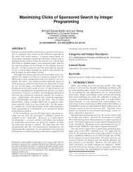
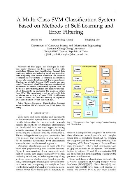
Document classificati<strong>on</strong> can be taken into two<br />
steps, text preprocessing and classifier training.<br />
Figure 1 is an overview <strong>of</strong> our document classificati<strong>on</strong><br />
system. Text preprocessing involves data<br />
retrieving techniques, includes segmenting a l<strong>on</strong>g<br />
sentence to serval shorter terms (word segmentati<strong>on</strong>),<br />
eliminating the meaningless keywords (feature<br />
extracti<strong>on</strong>), computing the weight <strong>of</strong> keywords<br />
(term weighting), and representing a document<br />
in Vector Space Model (VSM). In feature ex-<br />
Fig. 1. <str<strong>on</strong>g>SVM</str<strong>on</strong>g> system for Text Preprocessing ,<str<strong>on</strong>g>Class</str<strong>on</strong>g>ifier Training,<br />
and <str<strong>on</strong>g>Class</str<strong>on</strong>g>ificati<strong>on</strong>.<br />
tracti<strong>on</strong>, it computes the weights <strong>of</strong> all keywords,<br />
then eliminates some keywords with weights<br />
lower than a predefined threshold. To compute<br />
the weight <strong>of</strong> each keyword, three methods, Term<br />
Frequency (TF), Term Frequency * Inverse Document<br />
Frequency (TFIDF), and Informati<strong>on</strong> Gain<br />
(IG)[6], are adopted in our system. Two normalizati<strong>on</strong><br />
techniques, L1 and L2 normalizati<strong>on</strong>[16],<br />
are also applied in term weighting to compare the<br />
performance difference.<br />
Some well-known classificati<strong>on</strong> methods like<br />
K-Nearest Neighbors (KNN)[15], Support Vector<br />
Machines (<str<strong>on</strong>g>SVM</str<strong>on</strong>g>)[5][3][7], Naive Bayes[10], and<br />
neural network[14] have been well studied recently.<br />
We chooses <str<strong>on</strong>g>SVM</str<strong>on</strong>g> as our basic classifier
ecause <str<strong>on</strong>g>SVM</str<strong>on</strong>g> has been proven very effective in<br />
many research results and is able to deal with<br />
large dimensi<strong>on</strong>s <strong>of</strong> feature space. <str<strong>on</strong>g>SVM</str<strong>on</strong>g> is a statistic<br />
classificati<strong>on</strong> method proposed by Cortes and<br />
Vapnik in 1995 [7]. It is originally designed for<br />
binary classificati<strong>on</strong>. The derived versi<strong>on</strong>, a multiclass<br />
<str<strong>on</strong>g>SVM</str<strong>on</strong>g>, is a set <strong>of</strong> binary <str<strong>on</strong>g>SVM</str<strong>on</strong>g> classifiers able<br />
to classify a document to a specific class.<br />
In addicti<strong>on</strong> to use the basic classificati<strong>on</strong> techniques,<br />
we propose two revised methods, selflearning<br />
and error filtering, to increase the accuracy<br />
<strong>of</strong> multi-class <str<strong>on</strong>g>SVM</str<strong>on</strong>g> classificati<strong>on</strong>. The idea <strong>of</strong><br />
these two methods is as follows:<br />
1) The method <strong>of</strong> self-learning<br />
The classifier will retrain itself by combining<br />
the original training set and the misclassified<br />
documents to a new training set. This<br />
method avoids misclassifying similar documents<br />
again.<br />
2) The method <strong>of</strong> error filtering<br />
The system will identify documents which<br />
are difficult to be differentiated from all<br />
classes. If a document is marked as ”indistinct”,<br />
it means the document has high probability<br />
to be misclassified. To avoid misclassifying,<br />
the document should be reclassified<br />
by other classificati<strong>on</strong> methods.<br />
Our experiment uses 6000 <strong>of</strong>ficial documents<br />
<strong>of</strong> the Nati<strong>on</strong>al Chung Cheng University from<br />
the year 2002 to 2005. These documents have a<br />
comm<strong>on</strong>ly special property that there are seldom<br />
words in their c<strong>on</strong>tents. The average number <strong>of</strong><br />
keywords in each document is nearly 10. This<br />
leads to a challenge <strong>on</strong> the accuracy <strong>of</strong> the classificati<strong>on</strong><br />
system. In order to compare performance,<br />
our experiment implements several data retrieving<br />
techniques, TF, TFIDF, and IG as the feature<br />
extracti<strong>on</strong> scheme and TF, TFIDF with L1 and L2<br />
normalizati<strong>on</strong> as the term weighting scheme. We<br />
also adjust the filtering level <strong>of</strong> feature extracti<strong>on</strong><br />
to find out the best strategy. The filtering level<br />
is a percentage threshold <strong>of</strong> feature extracti<strong>on</strong>.<br />
The experiment shows the best strategy is to take<br />
IG with filtering level 0.9 as the scheme <strong>of</strong> feature<br />
extracti<strong>on</strong> and TFIDF with L2 normalizati<strong>on</strong><br />
as the scheme <strong>of</strong> term weighting. The accuracy<br />
is about 79.83%. When adopting the method <strong>of</strong><br />
self-learning, the average accuracy raises 1.64%.<br />
Adopting the method <strong>of</strong> error filtering, the average<br />
accuracy is up 4.45%. Combining the methods<br />
<strong>of</strong> self-learning and error filtering, the average<br />
accuracy improves 5.54% higher.<br />
The rest <strong>of</strong> the paper is organized as follows:<br />
Chapter 2 briefly introduces some multi-class<br />
<str<strong>on</strong>g>SVM</str<strong>on</strong>g> classificati<strong>on</strong>s. Chapter 3 presents the procedure<br />
<strong>of</strong> the classificati<strong>on</strong> system in this work.<br />
Chapter 4 presents the two methods <strong>of</strong> selflearning<br />
and error filtering. Chapter 5 shows the<br />
experiment performance <strong>of</strong> the classificati<strong>on</strong> system.<br />
Chapter 6 summarizes the main idea <strong>of</strong> this<br />
paper.<br />
II. RELATED WORKS<br />
The first process <strong>of</strong> classifying documents is<br />
to weight terms in documents. There are several<br />
popular methods like Mutual Informati<strong>on</strong> (MI),<br />
Chi Square Statistic (CHI), Term Frequency<br />
* Inverse Document Frequency (TFIDF),<br />
Informati<strong>on</strong> Gain (IG), etc. <str<strong>on</strong>g>Based</str<strong>on</strong>g> <strong>on</strong> these<br />
weights, it’s easier to decide which terms are<br />
significant and which terms should be filtered.<br />
Then, our classificati<strong>on</strong> procedure is to represent<br />
documents in Vector Space Model (VSM) and<br />
classify vectors by <str<strong>on</strong>g>SVM</str<strong>on</strong>g> classifier.<br />
Support Vector Machine (<str<strong>on</strong>g>SVM</str<strong>on</strong>g>) is a statistical<br />
classificati<strong>on</strong> system proposed by Cortes and Vapnik<br />
in 1995[7]. The simplest <str<strong>on</strong>g>SVM</str<strong>on</strong>g> is a binary<br />
classifier, which is mapping to a class and can<br />
identify an instance bel<strong>on</strong>ging to the class or not.<br />
To produce a <str<strong>on</strong>g>SVM</str<strong>on</strong>g> classifier for class C, the <str<strong>on</strong>g>SVM</str<strong>on</strong>g><br />
must be given a set <strong>of</strong> training samples including<br />
positive and negative samples. Positive samples<br />
bel<strong>on</strong>g to C and negative samples do not. After<br />
text preprocessing, all samples can be translated<br />
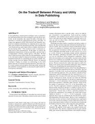
to n-dimensi<strong>on</strong>al vectors. <str<strong>on</strong>g>SVM</str<strong>on</strong>g> tries to find a<br />
separating hyper-plane with maximum margin to<br />
separate the positive and negative examples from<br />
the training samples.<br />
Fig. 2.<br />
Support vector machine<br />
There are two kinds <strong>of</strong> multi-class <str<strong>on</strong>g>SVM</str<strong>on</strong>g><br />
system[5], <strong>on</strong>e-against-all(OAA) and <strong>on</strong>e-against<strong>on</strong>e(OAO).<br />
The OAA <str<strong>on</strong>g>SVM</str<strong>on</strong>g> must train k binary<br />
<str<strong>on</strong>g>SVM</str<strong>on</strong>g>s where k is the number <strong>of</strong> classes. The<br />
ith <str<strong>on</strong>g>SVM</str<strong>on</strong>g> is trained with all samples bel<strong>on</strong>ging<br />
to ith class as positive samples, and takes other<br />
examples to be negative samples. These k <str<strong>on</strong>g>SVM</str<strong>on</strong>g>s<br />
could be trained in this way, and then k decisi<strong>on</strong><br />
functi<strong>on</strong>s are generated. After setting up all <str<strong>on</strong>g>SVM</str<strong>on</strong>g>s<br />
with positive and negative samples, it trains all<br />
k <str<strong>on</strong>g>SVM</str<strong>on</strong>g>s. Then it can get k decisi<strong>on</strong> functi<strong>on</strong>s.<br />
For a testing data, we compute all the decisi<strong>on</strong><br />
values by all decisi<strong>on</strong> functi<strong>on</strong>s and choose the<br />
2
maximum value and the corresp<strong>on</strong>ding class to<br />
be its resulting class.<br />
The class <strong>of</strong> input data x = arg max<br />
i=1...k (w i · x + b)<br />
The OAO <str<strong>on</strong>g>SVM</str<strong>on</strong>g> is that for every combinati<strong>on</strong> <strong>of</strong><br />
two classes i and j, it must train a corresp<strong>on</strong>ding<br />
SV M ij . Therefore, it will train k(k − 1)/2 <str<strong>on</strong>g>SVM</str<strong>on</strong>g>s<br />
and get k(k−1)/2 decisi<strong>on</strong> functi<strong>on</strong>s. For an input<br />
data, we compute all the decisi<strong>on</strong> values and use<br />
a voting strategy to decide which class it bel<strong>on</strong>gs<br />
to. If sign(w ij · x + b ij ) shows x bel<strong>on</strong>gs to ith<br />
class, then the vote for the ith class is added by<br />
<strong>on</strong>e. Otherwise, the jth class is added by <strong>on</strong>e.<br />
Finally, x is predicted to be the class with the<br />
largest vote. This strategy is also called the “Max<br />
Wins” method.<br />
There is no theoretic pro<strong>of</strong> that which kind<br />
<strong>of</strong> multi-class <str<strong>on</strong>g>SVM</str<strong>on</strong>g> is better, and they are <strong>of</strong>ten<br />
compared by experiment. In [5][16], it shows the<br />
average accuracy <strong>of</strong> OAA <str<strong>on</strong>g>SVM</str<strong>on</strong>g> is better than the<br />
OAO <str<strong>on</strong>g>SVM</str<strong>on</strong>g>.<br />
There are some researches for multi-class <str<strong>on</strong>g>SVM</str<strong>on</strong>g><br />
classificati<strong>on</strong>. In [16], it presents a new algorithm<br />
to deal with noisy training data, which combines<br />
multi-class <str<strong>on</strong>g>SVM</str<strong>on</strong>g> and KNN method. The result<br />
shows that this algorithm can greatly reduce the<br />
influence <strong>of</strong> noisy data <strong>on</strong> <str<strong>on</strong>g>SVM</str<strong>on</strong>g> classifier. In [9],<br />
it compares OAO <str<strong>on</strong>g>SVM</str<strong>on</strong>g>, OAA <str<strong>on</strong>g>SVM</str<strong>on</strong>g>, DAG <str<strong>on</strong>g>SVM</str<strong>on</strong>g><br />
(Directed Acyclic Graph <str<strong>on</strong>g>SVM</str<strong>on</strong>g>), and two all together<br />
<str<strong>on</strong>g>SVM</str<strong>on</strong>g>. An all together <str<strong>on</strong>g>SVM</str<strong>on</strong>g> means it trains<br />
a <str<strong>on</strong>g>SVM</str<strong>on</strong>g> classifier by solving a single optimizati<strong>on</strong><br />
problem. Experiments show that OAO and DAG<br />
method may be more suitable for practical use. In<br />
[8], it reduces training data by using KNN method<br />
before the procedure <strong>of</strong> <str<strong>on</strong>g>SVM</str<strong>on</strong>g> classificati<strong>on</strong>. The<br />
mean idea is to speed up the training time. The<br />
experiment compares OAO <str<strong>on</strong>g>SVM</str<strong>on</strong>g>, DAG <str<strong>on</strong>g>SVM</str<strong>on</strong>g>, and<br />
the proposed hybrid <str<strong>on</strong>g>SVM</str<strong>on</strong>g>. It shows the accuracy<br />
are similar for three methods but the training<br />
time <strong>of</strong> hybrid <str<strong>on</strong>g>SVM</str<strong>on</strong>g> outperforms the other two<br />
methods. In [12], it compares <str<strong>on</strong>g>SVM</str<strong>on</strong>g> and Naive<br />
Bayes in multi-class classificati<strong>on</strong>. They both use<br />
a method, called ”error correcting output code<br />
(ECOC)”, to decide the class label <strong>of</strong> input data.<br />
The experiment shows the accuracy <strong>of</strong> <str<strong>on</strong>g>SVM</str<strong>on</strong>g> is<br />
better than Naive Bayes method.<br />
III. CLASSIFICATION SYSTEM<br />
A classificati<strong>on</strong> system is composed <strong>of</strong> three<br />
phases, Text preprocessing, <str<strong>on</strong>g>SVM</str<strong>on</strong>g> training, and<br />
Performance testing.<br />
• Text preprocessing. Text preprocessing is<br />
taken into three steps, Word segmentati<strong>on</strong>,<br />
Feature extracti<strong>on</strong>, and Term weighting.<br />
1) Word segmentati<strong>on</strong>. First, l<strong>on</strong>g sentence<br />
should be segmented to several shorter<br />
terms. Especially, to segment Chinese<br />
sentence is much harder than English<br />
sentence because there is no natural delimiter<br />
between Chinese words. In our<br />
implementati<strong>on</strong>, we adopt a Chinese<br />
word segmentati<strong>on</strong> tool [18], developed<br />
by Institute <strong>of</strong> Informati<strong>on</strong> Science in<br />
Academia Sinica. The result <strong>of</strong> Chinese<br />
word segmentati<strong>on</strong> has large influence<br />
<strong>on</strong> accuracy for every kind <strong>of</strong> classificati<strong>on</strong><br />
system and the related studies are<br />
still proceeding.<br />
2) Feature extracti<strong>on</strong>. The following methods<br />
are implemented in our system.<br />
– TF, the weight <strong>of</strong> term i is defined as<br />
w(t i ) = tf i , where tf i is the number<br />
<strong>of</strong> occurrences <strong>of</strong> the ith term.<br />
– TFIDF, w(t i ) = tf i × log N n i<br />
, N is the<br />
number <strong>of</strong> all documents, n i is the<br />
number <strong>of</strong> documents where term i<br />
occurs.<br />
– IG,<br />
w(t i ) = −<br />
+p(t i )<br />
+p(̂t i )<br />
m∑<br />
p(c j ) log p(c j )<br />
j=1<br />
m∑<br />
p(c j |t i ) log p(c j |t i )<br />
j=1<br />
m∑<br />
p(c j |̂t i ) log p(c j |̂t i ) (1)<br />
j=1<br />
p(c j ) is the probability that category<br />
j occurs, p(t i ) is the probability that<br />
term i occurs, p(c j |t i ) is the probability<br />
that a document bel<strong>on</strong>g to category<br />
j if we know the term i occurs,<br />
p(̂t i ) is the probability that term i does<br />
not occur, p(c j |̂t i ) is the probability<br />
that a document bel<strong>on</strong>g to category j<br />
if we know the term i does not occur.<br />
It is difficult to define the threshold for<br />
the three methods. We use a percentage<br />
threshold instead, named filtering level<br />
(F L). Assume n is the number <strong>of</strong> keywords,<br />
let 0 < F L ≤ 1, then it reserves<br />
(n ∗ F L) keywords and eliminates the<br />
others. The remaining keywords are features<br />
and we use them to represent document<br />
vector. To simplify the notati<strong>on</strong>,<br />
we use TFIDF 0.8 to denote the TFIDF<br />
with filtering level 0.8.<br />
3) Term weighting. In practice, there are<br />
four combining methods are used<br />
– TF with L1 normalizati<strong>on</strong> (TF L1 ),<br />
d =( tf1<br />
S , tf2 tfn<br />
S<br />
, ... ,<br />
S ), where tf i is the<br />
number <strong>of</strong> occurrences <strong>of</strong> the ith term<br />
and S = ∑ n<br />
i=1 t i.<br />
3
– TF with L2 normalizati<strong>on</strong> (TF L2 ),<br />
d =( tf1<br />
S , tf2 tfn<br />
S<br />
, ... ,<br />
S ), where tf i is the<br />
number <strong>of</strong> occurrences <strong>of</strong> the ith term<br />
and S = √ ∑ n<br />
i=1 tf i 2.<br />
– TFIDF with L1 normalizati<strong>on</strong><br />
(TFIDF L1 ), d =( v1<br />
S , v 2<br />
v<br />
S<br />
, ... , nS<br />
),<br />
where v i = tf i × log N n i<br />
, N is the total<br />
number <strong>of</strong> documents in training set,<br />
n i is the number <strong>of</strong> documents in<br />
training set where term i occurs, and<br />
S = ∑ n<br />
i=1 tf i × log N n i<br />
.<br />
– TFIDF with L2 normalizati<strong>on</strong><br />
(TFIDF L2 ), d =( v1<br />
S , v 2<br />
v<br />
S<br />
, ... , nS<br />
),<br />
where v i = tf i × log N n i<br />
, N is the total<br />
number <strong>of</strong> documents in training set,<br />
n i is the number <strong>of</strong> documents in<br />
training set where term i occurs, and<br />
S =<br />
√ ∑n<br />
i=1 (tf i × log N n i<br />
) 2 .<br />
After text preprocessing, we can start<br />
training our classificati<strong>on</strong> system.<br />
• <str<strong>on</strong>g>SVM</str<strong>on</strong>g> training. The OAA <str<strong>on</strong>g>SVM</str<strong>on</strong>g> is chosen to be<br />
our classificati<strong>on</strong> system, i.e. k binary <str<strong>on</strong>g>SVM</str<strong>on</strong>g>s<br />
will be trained and an input data will be<br />
given the class with the maximum decisi<strong>on</strong><br />
value. C<strong>on</strong>sidering the performance <strong>of</strong> <str<strong>on</strong>g>SVM</str<strong>on</strong>g>,<br />
a <str<strong>on</strong>g>SVM</str<strong>on</strong>g> tool, <str<strong>on</strong>g>SVM</str<strong>on</strong>g> light [17], developed by<br />
Thorsten Joachims, will be adopted.<br />
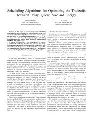
In <str<strong>on</strong>g>SVM</str<strong>on</strong>g> training, it first sets up all training<br />
data. For example, in figure 3, there are six<br />
documents in the training set. Document a1<br />
bel<strong>on</strong>gs to class A, document b1 and b2 bel<strong>on</strong>g<br />
to class B, and document c1, c2, and c3<br />
bel<strong>on</strong>g to class C. For the <str<strong>on</strong>g>SVM</str<strong>on</strong>g> classifier in C,<br />
a1 is in the positive set and other five documents<br />
bel<strong>on</strong>g to the negative set. For the <str<strong>on</strong>g>SVM</str<strong>on</strong>g><br />
classifier in B, b1 and b2 are in the positive<br />
set and other four documents bel<strong>on</strong>g to the<br />
negative set. For the <str<strong>on</strong>g>SVM</str<strong>on</strong>g> classifier in C, c1,<br />
c2, and c3 are in the positive set and other<br />
three documents bel<strong>on</strong>g to the negative set.<br />
Then <str<strong>on</strong>g>SVM</str<strong>on</strong>g> light is executed to train <str<strong>on</strong>g>SVM</str<strong>on</strong>g> A,B,<br />
and C and outputs three trained <str<strong>on</strong>g>SVM</str<strong>on</strong>g>s. We<br />
use the trained <str<strong>on</strong>g>SVM</str<strong>on</strong>g>s to classify documents.<br />
Fig. 3.<br />
Set up training set<br />
• Performance testing. In performance testing,<br />
it first weights terms with those features<br />
from feature extracti<strong>on</strong>. Then it uses the<br />
trained <str<strong>on</strong>g>SVM</str<strong>on</strong>g>s to classify documents. Every<br />
trained <str<strong>on</strong>g>SVM</str<strong>on</strong>g> will output a decisi<strong>on</strong> value.<br />
We choose the maximum decisi<strong>on</strong> value and<br />
corresp<strong>on</strong>ding class be the class <strong>of</strong> testing<br />
data. For a set <strong>of</strong> testing data, the way to<br />
evaluate accuracy is defined as<br />
number <strong>of</strong> correctly classified documents<br />
accuracy =<br />
number <strong>of</strong> total documents<br />
(2)<br />
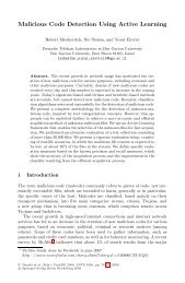
• An example <strong>of</strong> system flow.<br />
Fig. 4.<br />
An example <strong>of</strong> system flow<br />
Figure 4 is an example <strong>of</strong> system flow. At<br />
first, it needs a training set. Assume there<br />
are three documents d 1 , d 2 , and d 3 , and they<br />
bel<strong>on</strong>g to classes A, B, and C, respectively.<br />
1) Text preprocessing. L<strong>on</strong>g sentences<br />
should be first segmented to shorter<br />
terms. The Chinese word segmentati<strong>on</strong><br />
system from [18] is used in our<br />
implementati<strong>on</strong>. Assume there are six<br />
keywords (t 1 , t 2 , ..., t 6 ) after word<br />
segmentati<strong>on</strong> in our example. Then<br />
A : d 1 = (3, 5, 5, 0, 7, 0) means d 1 bel<strong>on</strong>gs<br />
to class A and c<strong>on</strong>tains 3t 1 , 5t 2 , 5t 3 and<br />
7t 5 . It uses TFIDF <strong>of</strong> feature extracti<strong>on</strong><br />
with filtering level 0.7 (TFIDF 0.7 ). The<br />
weight <strong>of</strong> t 1 = (3 + 3 + 3) × 3 3 = 9,<br />
the weight <strong>of</strong> t 2 = (5 + 1 + 0) × 3 2 = 9,<br />
and so <strong>on</strong>. Using the filtering level,<br />
6 × 0.7 = 4.2 ≃ 4 keywords will be<br />
reserved. After feature extracti<strong>on</strong>, it<br />
reserves t 1 , t 2 , t 3 and t 5 . Then TF<br />
with L1 normalizati<strong>on</strong> (TF L1 ) <strong>of</strong> term<br />
weighting is used. For example, the<br />
weight <strong>of</strong> t 1 in d 1 is<br />
3<br />
3+5+5+7 = 0.15.<br />
2) <str<strong>on</strong>g>SVM</str<strong>on</strong>g> training. The positive and negative<br />
samples for all <str<strong>on</strong>g>SVM</str<strong>on</strong>g>s should be set up.<br />
For example, <str<strong>on</strong>g>SVM</str<strong>on</strong>g> A takes all samples<br />
4
<strong>of</strong> class A {d 1 } to be positive set and all<br />
other samples {d 2 , d 3 } to be negative set.<br />
Then we use the <str<strong>on</strong>g>SVM</str<strong>on</strong>g> light [17] tool to be<br />
our classificati<strong>on</strong> system. It can help us<br />
train the <str<strong>on</strong>g>SVM</str<strong>on</strong>g>s correctly and efficiently.<br />
3) Performance testing. It first needs a testing<br />
set. Assume there are three testing<br />
documents d a , d b and d c and they bel<strong>on</strong>g<br />
to class A, B, and C, respectively. Using<br />
word segmentati<strong>on</strong> system to segment<br />
l<strong>on</strong>g sentences, and doing term weighting<br />
with those features that had been defined<br />
in feature extracti<strong>on</strong>, then we can<br />
classify three documents by all trained<br />
<str<strong>on</strong>g>SVM</str<strong>on</strong>g>s and get all decisi<strong>on</strong> values. We<br />
choose the maximum decisi<strong>on</strong> value and<br />
corresp<strong>on</strong>ding class to be the class <strong>of</strong><br />
input document. We can compute the accuracy<br />
and finish the performance testing.<br />
In our example, the decisi<strong>on</strong> values<br />
are given arbitrarily and the accuracy is<br />
66.67%.<br />
IV. THE IMPROVEMENT OF SYSTEM<br />
A. The method <strong>of</strong> self-learning<br />
When the classificati<strong>on</strong> system classifies some<br />
input data which classes has been known, the<br />
system can use those data to learn itself. Using<br />
all input data to retrain system leads to an<br />
inefficient system. Some specific data should be<br />
chosen and the misclassified data is a choice. The<br />
system would probably not misclassify the same<br />
or a similar data after retraining system by misclassified<br />
data. This method is called “Learning<br />
from Misclassified Data (LMD)”. The following<br />
describes the LMD.<br />
1) <str<strong>on</strong>g>Class</str<strong>on</strong>g>ify all testing data and return their<br />
classes.<br />
2) For every misclassified data <strong>of</strong> class A and<br />
its predicted class X, see figure 5, set it to<br />
the positive set <strong>of</strong> class A <str<strong>on</strong>g>SVM</str<strong>on</strong>g> and to the<br />
negative set <strong>of</strong> class X <str<strong>on</strong>g>SVM</str<strong>on</strong>g>.<br />
3) Retraining the <str<strong>on</strong>g>SVM</str<strong>on</strong>g>s which training set has<br />
been modified.<br />
It is a easy method and indeed can effectively<br />
increase the accuracy <strong>of</strong> the system.<br />
Fig. 5.<br />
Learning from Misclassified Data (LMD)<br />
B. The method <strong>of</strong> error filtering<br />
If there are k <str<strong>on</strong>g>SVM</str<strong>on</strong>g>s, an input data will have k<br />
decisi<strong>on</strong> values. We choose the class with maximum<br />
value to be the class <strong>of</strong> input data. But<br />
sometimes those decisi<strong>on</strong> values are all negative.<br />
It means the input data does not bel<strong>on</strong>g to any<br />
class and we still give it the class with maximum<br />
value. This could probably lead to misclassify.<br />
And sometimes the maximum and sec<strong>on</strong>d maximum<br />
values are very close. It means the input<br />
data is hard to be differentiated from the two most<br />
possible classes. This also may lead to misclassify.<br />
Our method avoids misclassifying documents.<br />
To avoid above situati<strong>on</strong>s, we define some<br />
thresholds for decisi<strong>on</strong> values. At first, for every<br />
input data, we evaluate two values, named<br />
Result Value (RV) and Difference Value (DV). RV<br />
is the maximum decisi<strong>on</strong> value which means<br />
how the input data is close to the corresp<strong>on</strong>ding<br />
class. DV is the difference between maximum<br />
and sec<strong>on</strong>d maximum value which means how<br />
the input data can be clearly separated from two<br />
most possible classes. Our method uses these two<br />
values to identify possibly misclassified data. The<br />
system returns the class or an indistinguishable<br />
message for an input data.<br />
Fig. 6.<br />
The distributi<strong>on</strong> <strong>of</strong> RV <strong>of</strong> documents<br />
We use figure 6 to describe the c<strong>on</strong>cept <strong>of</strong> our<br />
method. For all document which are classified<br />
to class A, figure 6 shows their distributi<strong>on</strong> <strong>of</strong><br />
RV. This distributi<strong>on</strong> is calculated by classifying<br />
a testing set and evaluating the average number<br />
<strong>of</strong> documents from four classes. The x-axis is<br />
RV and the y-axis is the number <strong>of</strong> documents.<br />
The solid line is the average number <strong>of</strong> correctly<br />
classified documents. The dotted line is the average<br />
number <strong>of</strong> misclassified documents. We can<br />
find that if a RV is larger than a threshold, for<br />
example threshold = 0, the input data has lots <strong>of</strong><br />
probability bel<strong>on</strong>ging to the corresp<strong>on</strong>ding class<br />
and we return the class straightforward in our<br />
method. We named the threshold “RV bound”<br />
5
(RVB). If the RV is smaller than RVB, we use DV<br />
to differentiate the document.<br />
the RVB, we use the documents which RVs are<br />
smaller than RVB to compute DVB. The formulati<strong>on</strong><br />
is defined as<br />
Fig. 7. The distributi<strong>on</strong> <strong>of</strong> DVs <strong>of</strong> documents which RVs are<br />
smaller than RVB<br />
DV B = Cor DV Avg × (1 −<br />
Cor Num′<br />
T otal ′ )<br />
Mis Num′<br />
+Mis DV Avg × (1 −<br />
T otal ′ ) (4)<br />
where Cor DV Avg is the average DV <strong>of</strong> correctly<br />
classified data, Cor Num ′ is the number<br />
<strong>of</strong> correctly classified data, Mis DV Avg is the<br />
average DV <strong>of</strong> misclassified data, Mis Num ′ is<br />
the number <strong>of</strong> misclassified data, and T otal ′ =<br />
Cor Num ′ + Mis Num ′ , i.e. the total number <strong>of</strong><br />
documents which RVs are smaller than RVB and<br />
are classified to class A.<br />
Figure 7 is the distributi<strong>on</strong> <strong>of</strong> DV which<br />
documents’ RVs are smaller than the RVB. In our<br />
method, if the DV is bigger than a threshold,<br />
named “Difference Value bound” (DVB), the<br />
system will return the class directly, or a<br />
indistinguishable message otherwise. Therefore,<br />
for an input data, the system will first identify<br />
it distinguishable or not and return the class if<br />
it is distinguishable or return a indistinguishable<br />
message otherwise. The following describes the<br />
rules.<br />
An input document is either distinguishable<br />
or indistinguishable.<br />
(a) Distinguishable<br />
1) RV ≥ RVB<br />
2) RV < RVB and DV ≥ DVB<br />
(b) Indistinguishable<br />
1) RV < RVB and DV < DVB<br />
Now the problem is how to define the two<br />
thresholds, RVB and DVB. For every binary classifier,<br />
we set RVB and DVB individually by learning<br />
from training data. At the first, it needs to classify<br />
all training data and gets RV and DV for every<br />
data. For a class A and all documents which are<br />
classified to class A, the RVB is computed by<br />
following formulati<strong>on</strong><br />
RV B = Cor RV Avg × (1 −<br />
Cor Num<br />
)<br />
T otal<br />
Mis Num<br />
+Mis RV Avg × (1 − ) (3)<br />
T otal<br />
where Cor RV Avg is the average RV <strong>of</strong> correctly<br />
classified data, Cor Num is the number <strong>of</strong> correctly<br />
classified data, Mis RV Avg is the average<br />
RV <strong>of</strong> misclassified data, Mis Num is the number<br />
<strong>of</strong> misclassified data, and T otal = Cor Num +<br />
Mis Num, i.e. the total number <strong>of</strong> documents<br />
which are classified to class A. After determining<br />
Fig. 8.<br />
An example <strong>of</strong> computing RVB and DVB<br />
The two formulati<strong>on</strong>s are the combinati<strong>on</strong>s <strong>of</strong><br />
average values <strong>of</strong> correctly classified and misclassified<br />
data by weighting both average values. The<br />
weight is proporti<strong>on</strong> to the inverse <strong>of</strong> percentage<br />
<strong>of</strong> the document number. The RVB and the DVB<br />
will clearly separate the correctly classified and<br />
misclassified data. Figure 8is an example <strong>of</strong> computing<br />
RVB and DVB. The left two columns is the<br />
RV and DV <strong>of</strong> correctly classified data. The right<br />
two columns is the RV and DV <strong>of</strong> misclassified<br />
data. The RVB and DVB can be calculated by the<br />
two formulati<strong>on</strong>s.<br />
C. Combining self-learning and error filtering<br />
In secti<strong>on</strong> IV, a method <strong>of</strong> self-learning, LMD<br />
is proposed. LMD chooses the misclassified data<br />
to retrain the system. But through separating<br />
6
indistinguishable data from the classified data,<br />
we have another way to choose which data to<br />
retrain the system. Because the predicted class<br />
<strong>of</strong> some indistinguishable data are correct, they<br />
should be learned. The indistinguishable data and<br />
misclassified data are combined for retraining the<br />
system. It is called “Learning from Misclassified<br />
and Indistinguishable Data (LMID)”. The following<br />
describes the LMID.<br />
1) <str<strong>on</strong>g>Class</str<strong>on</strong>g>ify all testing data and return their<br />
classes.<br />
2) For every misclassified data <strong>of</strong> class A and<br />
its predicted class X, see figure 9 and the<br />
dotted line, set it to the positive set <strong>of</strong> class<br />
A <str<strong>on</strong>g>SVM</str<strong>on</strong>g> and to the negative set <strong>of</strong> class X<br />
<str<strong>on</strong>g>SVM</str<strong>on</strong>g>.<br />
3) For every indistinguishable data <strong>of</strong> class A<br />
and its predicted class A, see figure 9 and the<br />
solid line, set it to the positive set <strong>of</strong> class A<br />
<str<strong>on</strong>g>SVM</str<strong>on</strong>g>.<br />
4) Retraining the <str<strong>on</strong>g>SVM</str<strong>on</strong>g>s which training set has<br />
been modified.<br />
The <strong>on</strong>ly difference between LMD and LMID<br />
is the step 3 in LMID. We compare the LMD and<br />
LMID in secti<strong>on</strong> V.<br />
Fig. 10. he accuracy <strong>of</strong> TF, TFIDF, and IG <strong>of</strong> feature extracti<strong>on</strong><br />
with TF L2 <strong>of</strong> term weighting<br />
Fig. 11. The accuracy <strong>of</strong> TF, TFIDF, and IG <strong>of</strong> feature<br />
extracti<strong>on</strong> with TFIDF L2 <strong>of</strong> term weighting<br />
Fig. 9. Learning from Misclassified and Indistinguishable<br />
Data (LMID).<br />
Figure 10 is the result <strong>of</strong> using TF L2 <strong>of</strong> term<br />
weighting and three kinds <strong>of</strong> feature extracti<strong>on</strong><br />
with increasing filtering level from 0 to 1. Figure<br />
11 is the result <strong>of</strong> using TFIDF L2 <strong>of</strong> term<br />
weighting. We can find out the IG is better than<br />
TFIDF and TF when filtering is decreasing but<br />
the differentiati<strong>on</strong> is not so obvious because <strong>of</strong><br />
the characteristic <strong>of</strong> seldom words <strong>of</strong> document<br />
c<strong>on</strong>tent.<br />
Then we compare TF L1 , TF L2 , TFIDF L1 , and<br />
TFIDF L2 <strong>of</strong> term weighting.<br />
V. EXPERIMENT RESULTS<br />
The experiment uses the <strong>of</strong>ficial documents <strong>of</strong><br />
the Nati<strong>on</strong>al Chung Cheng University from the<br />
year 2002 to 2005. We take 20 units (classes), 150<br />
documents for each unit (class) as training data,<br />
and 150 documents for each unit (class) as testing<br />
data. Totally we have 6000 documents for experiment.<br />
The input documents have a comm<strong>on</strong>ly<br />
special characteristic that they all have seldom<br />
words in their c<strong>on</strong>tents. The average number <strong>of</strong><br />
keywords is nearly 10 keywords in a document.<br />
This comm<strong>on</strong> property leads to a challenge <strong>on</strong> the<br />
accuracy <strong>of</strong> the classificati<strong>on</strong> system.<br />
The way to evaluate accuracy is defined as<br />
accuracy =<br />
number <strong>of</strong> correctly classified documents<br />
number <strong>of</strong> total documents<br />
Fig. 12. TF L1 , TF L2 , TFIDF L1 , and TFIDF L2 <strong>of</strong> term weighting<br />
with TF <strong>of</strong> feature extracti<strong>on</strong><br />
Figure 12, 13, and 14 are the results <strong>of</strong> comparing<br />
TF L1 , TF L2 , TFIDF L1 , and TFIDF L2 <strong>of</strong> term<br />
weighting with TF, TFIDF, and IG <strong>of</strong> feature<br />
extracti<strong>on</strong>. They show the TFIDF L2 outperforms<br />
7
Accuracy Basic <str<strong>on</strong>g>SVM</str<strong>on</strong>g> EF <str<strong>on</strong>g>SVM</str<strong>on</strong>g><br />
T1 0.8 0.8263<br />
T2 0.7817 0.8109<br />
T3 0.785 0.8185<br />
T4 0.77 0.7996<br />
T5 0.8017 0.8272<br />
Average 0.78168 0.8165<br />
TABLE II<br />
THE ACCURACY OF USING THE METHOD OF ERROR FILTERING<br />
(EF)<br />
Fig. 13. TF L1 , TF L2 , TFIDF L1 , and TFIDF L2 <strong>of</strong> term weighting<br />
with TFIDF <strong>of</strong> feature extracti<strong>on</strong><br />
Distinguish ability EF <str<strong>on</strong>g>SVM</str<strong>on</strong>g><br />
T1 0.95<br />
T2 0.9517<br />
T3 0.9367<br />
T4 0.0.9483<br />
T5 0.945<br />
Average 0.94634<br />
TABLE III<br />
THE DISTINGUISH ABILITY OF USING THE METHOD OF ERROR<br />
FILTERING (EF)<br />
Fig. 14. TF L1 , TF L2 , TFIDF L1 , and TFIDF L2 <strong>of</strong> term weighting<br />
with IG <strong>of</strong> feature extracti<strong>on</strong><br />
the others. The best strategy <strong>of</strong> the system for<br />
the input data is IG 0.9 <strong>of</strong> feature extracti<strong>on</strong> with<br />
TFIDF L2 <strong>of</strong> term weighting and the accuracy is<br />
79.83%.<br />
Table II is the result <strong>of</strong> using the method <strong>of</strong> selflearning<br />
(LMD) menti<strong>on</strong>ed in secti<strong>on</strong> IV-A. The<br />
testing data are divided into 5 sets. For each class,<br />
each set has 30 documents . Therefore, each set<br />
has totally 20 * 30 = 600 documents. We compare<br />
result with basic <str<strong>on</strong>g>SVM</str<strong>on</strong>g> and LMD <str<strong>on</strong>g>SVM</str<strong>on</strong>g>. Here we<br />
use the TFIDF L2 <strong>of</strong> term weighting and TF 1.0 <strong>of</strong><br />
feature extracti<strong>on</strong>. After classifying each testing<br />
data set, the system will automatically learn by<br />
itself. Therefore, beside <strong>of</strong> T1, the other testing<br />
sets will have different accuracy. We can find the<br />
average accuracy <strong>of</strong> LMD <str<strong>on</strong>g>SVM</str<strong>on</strong>g> is better than basic<br />
<str<strong>on</strong>g>SVM</str<strong>on</strong>g> and is 1.64% improvement <strong>on</strong> accuracy.<br />
Basic <str<strong>on</strong>g>SVM</str<strong>on</strong>g> LMD <str<strong>on</strong>g>SVM</str<strong>on</strong>g><br />
Data set Accuracy Accuracy<br />
T1 – –<br />
T2 0.7817 0.79<br />
T3 0.785 0.8017<br />
T4 0.77 0.7883<br />
T5 0.8017 0.81<br />
Average 0.7846 0.7975<br />
TABLE I<br />
THE ACCURACY OF USING THE METHOD OF SELF-LEARNING<br />
(LMD)<br />
Table IV-C and Table IV-C are the results <strong>of</strong><br />
using the method <strong>of</strong> error filtering(EF) menti<strong>on</strong>ed<br />
in secti<strong>on</strong> IV-B. We compare the “Basic <str<strong>on</strong>g>SVM</str<strong>on</strong>g>” and<br />
“EF <str<strong>on</strong>g>SVM</str<strong>on</strong>g>”, they show the average accuracy <strong>of</strong><br />
“Basic <str<strong>on</strong>g>SVM</str<strong>on</strong>g>” is 78.168%, and “EF <str<strong>on</strong>g>SVM</str<strong>on</strong>g>” is 81.65%<br />
with 94.634% distinguish ability. We can find that<br />
“EF <str<strong>on</strong>g>SVM</str<strong>on</strong>g>” has 4.45% improvement <strong>on</strong> average<br />
accuracy.<br />
Table IV-C and IV-C show the result <strong>of</strong> using<br />
the methods <strong>of</strong> combining error filtering and selflearning,<br />
which is menti<strong>on</strong>ed in secti<strong>on</strong> IV-C. We<br />
find that the accuracy and distinguish ability are<br />
both arising. LMD <str<strong>on</strong>g>SVM</str<strong>on</strong>g> and LMID <str<strong>on</strong>g>SVM</str<strong>on</strong>g> has<br />
5.54% and 5.24% improvement, respectively. The<br />
Accuracy Basic <str<strong>on</strong>g>SVM</str<strong>on</strong>g> EF <str<strong>on</strong>g>SVM</str<strong>on</strong>g> LMD EF <str<strong>on</strong>g>SVM</str<strong>on</strong>g> LMID EF <str<strong>on</strong>g>SVM</str<strong>on</strong>g><br />
T1 0.8 0.8263 0.8263 0.8263<br />
T2 0.7817 0.8109 0.8191 0.8134<br />
T3 0.785 0.8185 0.8473 0.847<br />
T4 0.77 0.7996 0.8277 0.8234<br />
T5 0.8017 0.8272 0.9363 0.8339<br />
Average 0.78168 0.8165 0.83134 0.82898<br />
TABLE IV<br />
THE ACCURACY OF USING THE METHOD OF COMBINING<br />
SELF-LEARNING AND ERROR FILTERING<br />
Distinguish ability EF <str<strong>on</strong>g>SVM</str<strong>on</strong>g> LMD EF <str<strong>on</strong>g>SVM</str<strong>on</strong>g> LMID EF <str<strong>on</strong>g>SVM</str<strong>on</strong>g><br />
T1 0.95 0.95 0.95<br />
T2 0.9517 0.94 0.467<br />
T3 0.9367 0.9167 0.915<br />
T4 0.9483 0.9383 0.9483<br />
T5 0.945 0.9467 0.9533<br />
Average 0.94634 0.93834 0.94266<br />
TABLE V<br />
THE DISTINGUISH ABILITY OF USING THE METHOD OF<br />
COMBINING SELF-LEARNING AND ERROR FILTERING<br />
8
accuracy <strong>of</strong> LMD is better than LMID <str<strong>on</strong>g>SVM</str<strong>on</strong>g> but<br />
LMID <str<strong>on</strong>g>SVM</str<strong>on</strong>g> has higher distinguish ability. So the<br />
difference between LMD <str<strong>on</strong>g>SVM</str<strong>on</strong>g> and LMID <str<strong>on</strong>g>SVM</str<strong>on</strong>g> is<br />
not obvious.<br />
VI. CONCLUSION<br />
In this paper, some data retrieving techniques,<br />
e.g. TF, TFIDF, and IG <strong>of</strong> feature extracti<strong>on</strong> and<br />
TF, TFIDF <strong>of</strong> term weighting with L1 and L2<br />
normalizati<strong>on</strong> are introduced. They can help us<br />
present a document or any kind <strong>of</strong> text. To classify<br />
a document, a classificati<strong>on</strong> system - multiclass<br />
<str<strong>on</strong>g>SVM</str<strong>on</strong>g> classifier is also introduced. By text<br />
preprocessing and <str<strong>on</strong>g>SVM</str<strong>on</strong>g> training, we can create a<br />
classificati<strong>on</strong> system and then automatically classify<br />
documents. The experiment shows the best<br />
strategy for the testing data is IG 0.9 <strong>of</strong> feature<br />
extracti<strong>on</strong> with TFIDF L2 <strong>of</strong> term weighting and<br />
the accuracy is 79.83%. The influence <strong>on</strong> feature<br />
extracti<strong>on</strong> is not obvious because <strong>of</strong> the characteristic<br />
<strong>of</strong> input documents, which have few<br />
keywords and 10 keywords <strong>on</strong> average. In order<br />
to improve the accuracy <strong>of</strong> the system, we propose<br />
two methods, the methods <strong>of</strong> self-learning<br />
and error filtering. By self learning (LMD), we<br />
found that the accuracy <strong>of</strong> LMD <str<strong>on</strong>g>SVM</str<strong>on</strong>g> has 1.64%<br />
improvement to the basic <str<strong>on</strong>g>SVM</str<strong>on</strong>g>. By error filtering<br />
(EF <str<strong>on</strong>g>SVM</str<strong>on</strong>g>), we can improve 4.45% <strong>on</strong> average<br />
accuracy . After combining the methods <strong>of</strong> selflearning<br />
and error filtering, the experiment shows<br />
the accuracy <strong>of</strong> LMD and LMID has 5.54% and<br />
5.24% improvement, respectively.<br />
VII. FUTURE WORKS<br />
In secti<strong>on</strong> II, we introduce some methods <strong>of</strong><br />
feature extracti<strong>on</strong> and there are also many other<br />
ways to do feature extracti<strong>on</strong>. We can add some<br />
new methods to the system and compare their<br />
results to find out the best <strong>on</strong>e. In secti<strong>on</strong> III,<br />
there is a short descripti<strong>on</strong> <strong>on</strong> word segmentati<strong>on</strong>.<br />
Chinese word segmentati<strong>on</strong> is hard especially and<br />
it has lots <strong>of</strong> chances to improve the influence <strong>of</strong><br />
word segmentati<strong>on</strong>. After filtering out some possibly<br />
misclassified data in secti<strong>on</strong> IV-C, the system<br />
does not deal with the filtered data. We can apply<br />
another kind <strong>of</strong> classifier to reclassify these data<br />
to improve the accuracy and distinguish ability.<br />
REFERENCES<br />
[1] Bernd Heisele, Purdy Ho, and Tomaso Poggio,<br />
”Face Recogniti<strong>on</strong> with Support Vector<br />
Machines: Global versus Comp<strong>on</strong>ent-based<br />
Approach”, IEEE Internati<strong>on</strong>al C<strong>on</strong>ference <strong>on</strong><br />
Computer Visi<strong>on</strong>, Vol. 2, pp.688-394, 2001.<br />
[2] Irene Diaz, Jose Ranilla, Elena M<strong>on</strong>tanes,<br />
Javier Fernandez, and Elias F. Combarro, ”Improving<br />
Performance <strong>of</strong> Text Categorizati<strong>on</strong><br />
by Combining Filtering and Support Vector<br />
Machines”, Journal <strong>of</strong> the American society<br />
for informati<strong>on</strong> science and technology, Vol.<br />
55(7), pp.579-542, 2004.<br />
[3] Nello Cristianini and John Shawe-Taylor, ”An<br />
Introducti<strong>on</strong> to Support Vector Machines and<br />
other kernel-based learning methods”, Cambridge<br />
University Press, 2000.<br />
[4] Elias F. Combarro, Elena M<strong>on</strong>tanes, Irene<br />
Diaz, Jose Ranilla, and Ricardo M<strong>on</strong>es, ”Introducing<br />
a Family <strong>of</strong> Linear Measures for Feature<br />
Selecti<strong>on</strong> in Text Categorizati<strong>on</strong>”, IEEE<br />
Transacti<strong>on</strong> <strong>on</strong> Knowledge and Data Engineering,<br />
vol. 17(9), pp.1223-1232, 2005.<br />
[5] Jiu-Zhen Liang, ”<str<strong>on</strong>g>SVM</str<strong>on</strong>g> multi-classifier and<br />
web document classificati<strong>on</strong>”, Internati<strong>on</strong>al<br />
C<strong>on</strong>ference <strong>on</strong> Machine Learning and Cybernetics,<br />
Vol.3 , pp.1347-1351, 2004.<br />
[6] Yiming Yang and Jan O. Pedersem, ”A Comparative<br />
Study <strong>on</strong> Feature Selecti<strong>on</strong> in Text<br />
Categorizati<strong>on</strong>”, Internati<strong>on</strong>al C<strong>on</strong>ference <strong>on</strong><br />
Machine Learning, pp.412-420, 1997.<br />
[7] C. Cortes and V. Vapnik, ”Support vector networks”,<br />
Machine learning, Vol. 20(3), pp.273-<br />
297, 1995.<br />
[8] Fu Chang, Chin-Chin Lin, and Chun-Jen<br />
Chen, ”A Hybrid Method for <str<strong>on</strong>g>Multi</str<strong>on</strong>g>class <str<strong>on</strong>g>Class</str<strong>on</strong>g>ificati<strong>on</strong><br />
and Its Applicati<strong>on</strong> to Handwritten<br />
Character Recogniti<strong>on</strong>”, Institute <strong>of</strong> Informati<strong>on</strong><br />
Science, Academia Sinica, Taipei, Taiwan,<br />
Tech. Rep. TR-IIS-04-016, 2004.<br />
[9] Chih-Wei Hsu and Chih-Jen Lin, ”A Comparis<strong>on</strong><br />
<strong>of</strong> Methods for <str<strong>on</strong>g>Multi</str<strong>on</strong>g>class Support Vector<br />
Machines”, IEEE Transacti<strong>on</strong> <strong>on</strong> Neural Networks,<br />
vol. 13(2), pp.425-425, 2002.<br />
[10] D. D. Lewis, ”Naive (Bayers) at forty: The<br />
independence assumpti<strong>on</strong> in informati<strong>on</strong> retrieval”,<br />
European C<strong>on</strong>ference <strong>on</strong> Machine<br />
Learning, pp.4-15 , 1998.<br />
[11] Andrew Moore, ”Statistical Data Mining Tutorials”,<br />
http://www.aut<strong>on</strong>lab.org/tutorials/<br />
[12] Jas<strong>on</strong> D. M. Rennie and Ryan Rifkin, ”Improving<br />
<str<strong>on</strong>g>Multi</str<strong>on</strong>g>class Text <str<strong>on</strong>g>Class</str<strong>on</strong>g>ificati<strong>on</strong> with<br />
the Support Vector Machine”, Massachusetts<br />
Institute <strong>of</strong> Technology, Artificial Intelligence<br />
Laboratory Publicati<strong>on</strong>s, AIM-2001-026, 2001.<br />
[13] G. Salt<strong>on</strong> and C. Buckley, ”Term weighting<br />
approaches in automatic text retrieval”, Informati<strong>on</strong><br />
Processing and Management, Vol.<br />
24(5), pp.513-523, 1988.<br />
[14] E Wiener, ”A neural network approach to<br />
topic spotting”, Symposium <strong>on</strong> Document<br />
Analysis and Informati<strong>on</strong> Retrieval, pp. 317-<br />
332, 1995.<br />
[15] Fang Yuan, Liu Yang, and Ge Yu, ”Improving<br />
9
The K-NN and Applying it to Chinese Text<br />
<str<strong>on</strong>g>Class</str<strong>on</strong>g>ificati<strong>on</strong>”, Internati<strong>on</strong>al C<strong>on</strong>ference <strong>on</strong><br />
Machine Learning and Cybernetics, Vol. 3, pp.<br />
1547-1553, 2005.<br />
[16] Jia-qi Zou, Guo-l<strong>on</strong>g Chen, and Wen-zh<strong>on</strong>g<br />
Guo, ”Chinese Web Page <str<strong>on</strong>g>Class</str<strong>on</strong>g>ificati<strong>on</strong> Using<br />
Noise-tolerant support vector Machines”,<br />
IEEE Internati<strong>on</strong>al C<strong>on</strong>ference <strong>on</strong> Natural<br />
Language Processing and Knowledge Engineering,<br />
pp.785-790 , 2005.<br />
[17] <str<strong>on</strong>g>SVM</str<strong>on</strong>g> light , http://svmlight.joachims.org/<br />
[18] The Chinese Knowledge and Informati<strong>on</strong><br />
Processing (CKIP) <strong>of</strong> Academia Sinica <strong>of</strong> Taiwan,<br />
A Chinese word segmentati<strong>on</strong> system,<br />
http://ckipsvr.iis.sinica.edu.tw/<br />
10