Magnetic and transport properties of ferromagnetic semiconductor ...

Magnetic and transport properties of ferromagnetic
semiconductor multinary alloys
Pb 1−x−y−z Mn x Eu y Sn z Te and Ga 1−x Mn x As
Izabela Kudelska
PhD Dissertation
Institute of Physics
Polish Academy of Sciences
Thesis Supervisor doc. dr. hab. W. Dobrowolski
Warsaw 2004

Mojemu kochanemu Synkowi Olesiowi,
który towarzyszył mi
przez cały okres pisania pracy

PODZI ˛ EKOWANIA
Pragnę serdecznie podziękować mojemu Promotorowi doc. dr hab. W. Dobrowolskiemu
za stałą, wszechstronną pomoc i opiekę nad pracą, pouczające rozmowy i życzliwość
w trakcie wykonywania pracy.
Prof. dr J. Furdynie bardzo dziękuję za inspirujące dyskusje i wprowadzenie w tematykę
badań ferromagnetycznych kryształów Ga 1−x Mn x As.
Prof. dr M. Dobrowolskiej dziękuję bardzo za opiekę i pomoc w badaniach.
Dr M. Arciszewskiej serdecznie dziękuję za pomoc przy wykonywaniu pracy i życzliwe
zainteresowanie wynikami badań.
Doc. dr hab. T. Wojtowiczowi dziękuję bardzo za wyhodowanie kryształów Ga 1−x Mn x As
użytych do badań i pomoc przy powstawaniu pracy.
Pragnę podziękować dr X. Liu za pomiary namagnesowania oraz wyhodowanie kryształów
Ga 1−x Mn x As, W. Lim za pomoc w badaniach transportowych oraz dr Y. Sasaki za
wyhodowanie kryształów Ga 1−x Mn x As badanych w pracy.
Współpraca z pracownikami Laboratorium Silnych Impulsowych Pól Magnetycznych w
Tuluzie była bardzo pomocna. W szczególności pragnę podziękować dr O. Portugall za
pomoc w pomiarach magnetotransportowych, dr M. Goiran za pomoc w pomiarach magnetooptycznego
efektu Kerra, a także dr E.Haanappel, dr J.-M. Broto, dr H. Rakoto, dr B.
Raquet za pomoc w pomiarach magnetotransportowych.
Pragnę także podziękować Prof. dr V. Dugaev za cenne i inspirujące dyskusje.
Prof. dr W. Walukiewiczowi oraz dr K. M. Yu dziękuję za pomiary c-PIXE oraz c-RBS.
Bardzo dziękuję dr J. Domagale za pomiary dyfrakcji rentgenowskiej.
Dr E. I. Slynko oraz dr V. E. Slynko dziękuję za wyhodowanie kryształów
Pb 1−x−y−z Mn x Eu y Sn z Te użytych do badań.
Dr I. M. Fita dziękuję za pomiary namagnesowamia w ciśnieniu hydrostatycznym.
Pragnę także podziękować Prof. dr hab. R. Szymczak oraz dr Baranowi za pomiary namagnesowania.
Wszystkim pracownikom i doktorantom z Odziału Fizyki Półprzewodników Półmagnetycznych
dziękuję za stworzenie miłej i życzliwej atmosfery.
Mojemu Mężowi Arkowi pragnę podziękować za nieustanne wspieranie mnie i cierpliwość.
3

CONTENTS
1. Introduction . . . . . . . . . . . . . . . . . . . . . . . . . . . . . . . . . . . 6
2. Experimental techniques . . . . . . . . . . . . . . . . . . . . . . . . . . . . . 10
2.1 Introduction . . . . . . . . . . . . . . . . . . . . . . . . . . . . . . . . . 10
2.2 The experimental technique of energy dispersive X-ray fluorescence
(EDXRF) . . . . . . . . . . . . . . . . . . . . . . . . . . . . . . . . . . 11
2.3 The experimental setup for magnetotransort measurements . . . . . . . . 12
2.4 AC/DC magnetometer . . . . . . . . . . . . . . . . . . . . . . . . . . . 13
2.5 The measurements in the range of high pulsed magnetic fields . . . . . . 18
2.6 The experimental setup for Kerr effect measurements . . . . . . . . . . . 19
3. Samples of Pb 1−x−y−z Mn x Eu y Sn z Te and Ga 1−x Mn x As. . . . . . . . . . . . . 21
3.1 Ferromagnetic bulk crystals of Pb 1−x−y−z Mn x Eu y Sn z Te . . . . . . . . . 21
3.2 Ferromagnetic layers of Ga 1−x Mn x As. . . . . . . . . . . . . . . . . . . . 21
4. Transport and magnetic investigations of Pb 1−x−y−z Mn x Eu y Sn z Te . . . . . . . 27
4.1 Introduction . . . . . . . . . . . . . . . . . . . . . . . . . . . . . . . . . 27
4.2 Transport characterization of Pb 1−x−y−x Mn x Eu y Sn z Te samples . . . . . . 30
4.3 Magnetic measurements of Pb 1−x−y−z Mn x Eu y Sn z Te mixed crystals . . . 34
5. Low temperature annealing studies of Ga 1−x Mn x As . . . . . . . . . . . . . . . 48
5.1 Introduction . . . . . . . . . . . . . . . . . . . . . . . . . . . . . . . . . 48
5.2 The procedure of annealing . . . . . . . . . . . . . . . . . . . . . . . . . 51
5.3 The results of zero-field resistivity measurements . . . . . . . . . . . . . 51
5.4 The results of magnetotransport measurements . . . . . . . . . . . . . . 56
5.5 The results of SQUID measurements . . . . . . . . . . . . . . . . . . . . 64
5.6 The results of magnetooptical Kerr effect measurements . . . . . . . . . . 69
5.6.1 Introduction - magnetooptical Kerr effect . . . . . . . . . . . . . 69
5.6.2 The results of MOKE measurements for the as-grown and annealed
GaMnAs epilayers . . . . . . . . . . . . . . . . . . . . . 71
5.7 The channeling experiments - the results of c-RBS and c-PIXE measurements
. . . . . . . . . . . . . . . . . . . . . . . . . . . . . . . . . . . . 84
5.8 The results of diffraction (HRXRD) measurements . . . . . . . . . . . . 90
6. Conclusions and Summary . . . . . . . . . . . . . . . . . . . . . . . . . . . . 99
6.1 Pb 1−x−y−z Mn x Eu y Sn z Te . . . . . . . . . . . . . . . . . . . . . . . . . . 99
6.2 Ga 1−x Mn x As . . . . . . . . . . . . . . . . . . . . . . . . . . . . . . . . 99
6.3 Suggestions for further studies . . . . . . . . . . . . . . . . . . . . . . . 101

Contents 5
7. Appendices . . . . . . . . . . . . . . . . . . . . . . . . . . . . . . . . . . . 103
7.1 Appendix 1 . . . . . . . . . . . . . . . . . . . . . . . . . . . . . . . . . 103
7.2 Appendix2 . . . . . . . . . . . . . . . . . . . . . . . . . . . . . . . . . . 105
Bibliography . . . . . . . . . . . . . . . . . . . . . . . . . . . . . . . . . . . . . 110
List of Figures . . . . . . . . . . . . . . . . . . . . . . . . . . . . . . . . . . . . 116
List of Tables . . . . . . . . . . . . . . . . . . . . . . . . . . . . . . . . . . . . 122

1. INTRODUCTION
In this thesis, the results of a study of the magnetic and transport properties of III-V as
well as IV-VI based ferromagnetic semimagnetic semiconductors will be presented. Two
systems of ferromagnetic semiconductor multinary alloys: PbSnMnEuTe and GaMnAs
were systematically investigated.
The common characteristic of two investigated semimagnetic materials,
Ga 1−x Mn x As and Pb 1−x−y−z Mn x Eu y Sn z Te, is mediation of free holes in ferromagnetic
interactions of Mn ions. The mechanism of exchange interactions is well explored
for Pb 1−x−y Mn x Sn y Te mixed crystals. The RKKY interaction is known to be responsible
for the ferromagnetic properties of IV-VI semimagnetic semiconductors. However,
the origin of ferromagnetism in Ga 1−x Mn x As is still under active discussion. The
experimental studies of physical properties are necessary to examination the origin of
ferromagnetism in this material.
Recently, manipulation of the spin degree of freedom in semiconductors has become
a focus of interest. The main goal of spintronics is to make use of both charge and spin
degrees of freedom in semiconductors. In the context of spin electronics particularly
interesting are ferromagnetic semimagnetic semiconductors. In the case of Mn-based IV-
VI, III-V and II-VI SMSC’s the ferromagnetism can be observed provided that the hole
concentration is sufficiently high.
Understanding of the carrier mediated ferromagnetism was initiated by a study of
ferromagnetism in IV-VI based SMSC’s. In this class of materials deviations from stoichiometry
result in the carrier density sufficiently high to produce strong ferromagnetic
interactions between the localized spins. Ferromagnetic properties are observed for IV-
VI semimagnetic materials with Mn and with the concentration of conducting holes p
≥ 2-3 10 20 cm −3 . However, in the case of ferromagnetic IV-VI semimagnetic materials
(such as PbSnMnTe), one have to admit that the ferromagnetic characteristics (magnetic
anisotropy, coercive field) are not superior to other magnetic materials. Thus, applications
related to ferromagnetic properties of these materials can be rather related to hybrid
systems with IV-VI electronic devices incorporating the ferromagnetic element with controlled
magnetic properties. An additional obstacle for these materials is the low temperature
of ferromagnetic phase transition. However, two important features give IV-VI semimagnetic
materials the distinguished position within the whole family of semimagnetic
semiconductors. First, the variety of magnetic properties observed in Mn based IV-VI
SMSC’s. Second, the characteristic feature are semi-metallic electric properties with the
well developed methods of control of carrier concentration. Pb 1−x−y−z Mn x Eu y Sn z Te are
a unique compounds in which the interplay between magnetic and electronic properties
can be observed and studied. Particularly, the carrier induced paramagnet-ferromagnet
and ferromagnet-spin glass transitions are present [1], [2].
Recently, due to the rapid progress achieved in SMSC’s technology, namely nonequilibrium
growth methods, the ferromagnetic phase transition was observed in III-V

1. Introduction 7
semimagnetic materials. For the first time, by using low-temperature molecular beam
epitaxy (LT-MBE; T < 300 0 C), a III-V based SMSC, In 1−x Mn x As layers were successfully
grown in 1989 [3] and shown to exhibit hole-induced ferromagnetic ordering at
low temperatures. Development of this technique resulted in the successful epitaxy of
Ga 1−x Mn x As [4], [5]. The III-V based compounds are prospective materials for spin
electronics because are already in use in everyday electronics. The low temperature (LT)
MBE grown Ga 1−x Mn x As, has become a favorite material for spintronics when it was
shown [6] that the substitution of Mn for Ga in GaAs leads to ferromagnetism at temperatures
as high as 110K. For a long time this was the highest Curie temperature T C
observed in semimagnetic semiconductors. For the spintronic applications, however, the
temperature of the transition to the ferromagnetic phase has to be considerable increased.
In this thesis, the systematic measurements of magnetic AC susceptibility, magnetization
as well as transport characterization of bulk samples of Pb 1−x−y−z Mn x Eu y Sn z Te
multinary alloy were performed. The as-grown as well as annealed samples with different
concentration of Mn x as well as Eu y were investigated. The paramagnet-ferromagnet as
well as ferromagnet-spin glass transitions were observed and studied. The results of magnetic
and transport studies showed that by introducing of two types of magnetic ions into
IV-VI semiconductor matrix, one can change the magnetic properties of the investigated
semimagnetic material.
The variety of experimental techniques were used to explore the physical properties of
Ga 1−x Mn x As epilayers. The transport, magnetotransport, magnetic, structural as well as
channelling experiments were carried out and analyzed. The magnetooptical Kerr effect
studies allowed to explore the magnetooptical properties of the investigated samples. The
as-grown as well as annealed at various conditions samples were investigated. The main
subject studied is the role of Mn interstitial in Ga 1−x Mn x As epilayers. The magnetic,
transport, structural and channeling experiments indicated that the formation of interstitial
Mn ions plays a crucial role in controlling the ferromagnetic transition in GaMnAs. For
the first time it is shown that by a proper choice of annealing conditions (temperature,
time, flow of the gas) the limit of the Curie temperature of Ga 1−x Mn x As epilayers (T C
∼ 110K) can be shifted to much higher values (up to 127K for the sample with high Mn
concentration x ∼ 0.08) [7]. The results presented in the thesis initiated further studies of
low temperature annealing in many laboratories. At present, Curie temperature exceeding
160K was reported [8]. This progress has been achieved basically though optimization of
post-growth annealing time and temperature.
The variety of experimental techniques were used in the studies presented in the thesis.
The measurements of energy dispersive X-ray fluorescence (EDXRF), magnetotransport
studies (up to 13T using superconducting magnet), AC magnetic susceptibility as well
as DC magnetization (up to 9T) by use of 7229 LakeShore Susceptometer/Magnetometer
setup were performed in Division ON-1 Physics of Semiconductors of Institute of Physics
Polish Academy of Sciences in Warsaw.
The results were obtained in collaboration with many groups. The XRD as well as
RHEED measurements were carried out in Department of Physics, University of Notre
Dame. High resolution X-ray diffraction studies as well as the standard powder X-ray
measurements were performed in Laboratory of X-ray and Electron Microscopy Research,
Group of Applied Crystalography, Institute of Physics Polish Academy of Sciences
in Warsaw.
The transport as well as magnetotransport investigations in the static magnetic field

1. Introduction 8
were carried out in Department of Physics, University of Notre Dame (up to 0.5T by use
of classical electromagnet; up to 5T by use of superconducting magnet). The magnetotransport
measurements in high pulsed magnetic fields (up to 55T) were performed in
Laboratoire National des Champs Magnetiques Pulses Toulouse.
The magnetization measurements under hydrostatic pressure were carried out in Division
of Physics of Magnetism, Group of Phase Transitions, Institute of Physics Polish
Academy of Sciences in Warsaw. The SQUID measurements were performed in Department
of Physics, University of Notre Dame and Division of Physics of Magnetism, Group
of Phase Transitions, Institute of Physics Polish Academy of Sciences in Warsaw. Indirect
magnetization measurements were also performed. The magnetooptical Kerr Effect
(MOKE) was measured in high pulsed magnetic fields (up to 25T) in Laboratoire National
des Champs Magnetiques Pulses Toulouse.
The channeling experiments i.e. channeling Rutherford backscattering (c-RBS) and
channeling particle-induced X-ray emission (c-PIXE) measurements were performed in
Material Science Division Lawrence Berkeley National Laboratory.
The thesis is organized in the following way. Chapter 1 describes selected experimental
techniques used in the studies. The characterization of the samples is given in Chapter
2. The results of transport and magnetic measurements of Pb 1−x−y−z Mn x Eu y Sn z Te crystals
are presented and analyzed in Chapter 3. The results of experimental studies of LT
Ga 1−x Mn x As epilayers: the procedure of annealing, the results of zero-field resistivity,
magnetotransport, magnetic, channelling as well as structural measurements are presented
and discussed in Chapter 4. The summary and outlook is given in Chapter 5.
The results presented in this thesis were partially published in the papers:
1. Kuryliszyn I., Arciszewska M., Abdel Aziz M.M., Slynko E.I., Slynko V.I., Dugaev
V.K., "In quest of Mn-Eu interaction in IV-VI mixed crystals", Proc. 9th Int. Conf.
On Narrow Gap Semiconductors, ed. by N. Puhlman, H.-U. Müller, M. Von Ortenberg,
Humboldt University Berlin, p. 96-98 (2000).
2. Yu K.M., Walukiewicz W., Wojtowicz T., Kuryliszyn I., Liu X., Sasaki Y., Furdyna
J.K., "Effect of the location of Mn sites in ferromagnetic Ga 1−x Mn x As on its Curie
temperature", Phys. Rev. B, vol.65, p. 201303(R), (2002).
3. Kuryliszyn I., Wojtowicz T., Liu X., Furdyna J., Dobrowolski W., Broto J.-M., Goiran
M., Portugall O., Rakoto H., Raquet B., Transport and magnetic properties of LT
annealed Ga 1−x Mn x As", Acta Phys. Pol. A, vol.102, No 4-5, p.659, (2002).
4. Kuryliszyn I., Wojtowicz T., Liu X., Furdyna J.K., Dobrowolski W., Broto J.-M.,
Goiran M., Portugall O., Rakoto H., Raquet B., "Low Temperature annealing
studies of Ga 1−x Mn x As", Journal of Supercondactivity (Incorporating Novel Magnetism),
vol. 16, No 1, p. 63, (2003).
5. Yu K.M., Walukiewicz W., Wojtowicz T., Kuryliszyn I., Liu X., Sasaki Y., Furdyna
J.K., "Thermodynamic Limits to the maximum Curie Temperature in GaMnAs",
Proceedings- 26th International Conference on the Physics of semiconductors, Edinburgh
2002.

1. Introduction 9
6. Racka K., Kuryliszyn I., Arciszewska M., Dobrowolski W., Broto J.-M., Goiran M.,
Portugall O., Rakoto H., Raquet B., " Anomalous Hall Effect in Sn 1−x−y Mn x Eu y Te
Mixed Crystals", Journal of Supercondactivity, (Incorporating Novel Magnetism),
vol. 16, No 2, p. 289, (2003).
7. Furdyna J.K., Liu X., Lim W.L., Sasaki Y., Wojtowicz T., Kuryliszyn I., Lee S., Yu
K.M. and Walukiewicz W., "Ferromagnetic III-Mn-V Semiconductors: Manipulation
of Magnetic Properies by Annealing, Extrinsic Doping, and Multilayer Design",
Journal of the Korean Physical Society, vol. 42, p. S579, (2003).
8. Kuryliszyn-Kudelska I., Domagala J.Z, Wojtowicz T., Liu X., E. Łusakowska, Dobrowolski
W., Furdyna J.K., "The effect of Mn interstitials on the lattice parameter
of Ga 1−x Mn 1−x As", J. Appl. Phys. 95 (2) 603 (2004).
9. Kuryliszyn-Kudelska I., Wojtowicz T., Liu X., Furdyna J.K., Dobrowolski W., Domagala
J.Z., E.Łusakowska, M.Goiran, E.Haanappel, O. Portugall, "Effect of annealing
on magnetic and magnetotransport properties of Ga 1−x Mn x As epilayers",
Journal of Magnetic Materials and Magnetism 272-276, p. e1575, (2004).
10. Kacman P., Kuryliszyn-Kudelska I., "The role of Interstitial Mn in GaAs-based Dilute
Magnetic Semiconductors", Lecture Notes in Physics (in press)

2. EXPERIMENTAL TECHNIQUES
2.1 Introduction
Chapter 2 includes briefly description of the selected experimental methods which were
used by author.
The chemical composition of the investigated samples was determined by use of
different techniques. The X-ray dispersive fluorescence analysis measurements (for
Pb 1−x−y−z Mn x Eu y Sn z Te samples), X-ray diffraction (XRD) as well as high resolusion X-
ray diffraction (HRXRD) studies and reflection high energy electron diffraction (RHEED)
measurements (for Ga 1−x Mn x As epilayers) were employed to characterize the investigated
samples. Section 1.1 contains briefly description of Tracor X-ray Spectrace 5000 -
automated EDXRF analyzer.
The structural characterization of both - Pb 1−x−y−z Mn x Eu y Sn z Te as well as
Ga 1−x Mn x As epilayers was carried out. X-ray diffraction (Ga 1−x Mn x As samples), high
resolution X-ray diffraction (Ga 1−x Mn x As samples) and standard powder X-ray measurements
(Pb 1−x−y−z Mn x Eu y Sn z Te samples) were performed.
The transport (resistivity) as well as magnetotransport (Hall effect, anomalous Hall
effect, magnetoresistance) properties of investigated ferromagnetic materials were studied
by use of several experimental setups. The resistivity measurements of Ga 1−x Mn x As
samples were performed in the temperature range between 10K and 300K by use of a
helium flow cryostat. The DC six probe technique was used for the magnetotransport
measurements. Section 2.2 describes the experimental setup for magnetotransport measurements
built by author in Department of Physics University of Notre Dame. The system
together with the cryostat and superconducting magnet allows to perform the standard
DC six probe technique measurements in magnetic field up to 5T and in the temperature
range between 1.3 and 300K. Section 3 of this Chapter describes briefly pulsed magnetic
fields.
The magnetic studies (AC susceptibility and magnetization investigations) were performed
by use of several techniques. The Pb 1−x−y−z Mn x Eu y Sn z Te samples were explored
using AC/DC magnetometer - AC susceptibility as well as DC magnetization (up
to 9T) were measured. The principle of operation and schematic figures of the 7229
LakeShore Susceptometer/Magnetometer setup are shown in Section 2.4. Additionally,
the magnetization measurements under hydrostatic pressure were performed using the vibrating
sample magnetometer for Pb 1−x−y−z Mn x Eu y Sn z Te samples. For Ga 1−x Mn x As
epilayers magnetization studies were performed. First, directly magnetization investigation
were carried out by use of SQUID magnetometer. Second, magnetoptical Kerr effect
(MOKE) were performed. The experimental setup for MOKE measurements is described
in section 2.5.
The channeling experiments - channeling particle-induced X-ray emission (c-PIXE)
as well as channeling Rutherford backscattering (c-RBS) were performed for GaMnAs

2. Experimental techniques 11
samples. The principle of channeling experiments is briefly described in Section 7 of
Chapter 5.
2.2 The experimental technique of energy dispersive X-ray fluorescence
(EDXRF)
The chemical composition of IV-VI semimagnetic semiconductors was determined by X-
ray dispersive fluorescence analysis technique. This technique allows for determination of
chemical composition of the samples with uncertainty of 10 %. The experimental setup -
X-ray beam geometry is shown schematically in Figure 2.1. The Tracor X-ray Spectrace
5000 is an automated energy dispersive X-ray fluorescence (EDXRF) analyzer. It can be
used for nondestructive elemental analysis of solids and liquids.
Fig. 2.1: The schematic view of the Tracor X-ray Spectrace 5000.
The principle of operation is very simple. The primary X-rays from X-ray tube hit
the sample and induce the emission of secondary X-rays by the elements contained in the
sample.
The relative intensity of an X-ray spectral line excited by monochromatic radiation
can be computed for a given element and known spectrometer geometry using following
equation:
I L = I 0 ω A g L
r A − 1
r A
dΩ
4π
C A µ A (λ pri ) csc(φ)
µ M (λ pri ) csc(φ) + µ M (λ L ) csc(Φ)
where:
I L is the analyte line intensity
I 0 is the intensity of the primary beam with effective wavelength λ pri
λ pri is the effective wavelength of the primary X-ray
λ L is the wavelength of the measured analyte line
g L is the fractional value of the measured analyte line L in its series
(2.1)

2. Experimental techniques 12
r A is the absorption edge jump ratio of analyte A
C A is the concentration of analyte A
dΩ/4π is the fractional value of the fluorescent X-ray that is directed toward a detector
µ A (λ pri ) is the mass absorption coefficient of analyte A for λ pri
µ M (λ pri ) is the mass absorption coefficient of the matrix for λ pri
µ M (λ L ) is the mass absorption coefficient of the matrix for analyte line λ L
φ is the incident angle of the primary beam
Φ is the takeoff angle of fluorescent beam
The Spectrace 5000 uses a low power X-ray tube (less than 50 watts) with a rhodium
anode target. The X-ray tube generates the X-rays that are incident upon the sample so
as to cause the sample to fluorescence. The X-rays emitted by the anode pass through a
0.005" Beryllium window. Then the beam is collimated and filtered. The collimator and
X-ray tube define the illumination beam. To minimize scattering, the detector acceptance
is 90 0 from the incident beam. The sample is placed at the intercept of the two beams as
is shown in Figure 2.1. Liquid nitrogen inside a dewar cools the Si(Li) detector to reduce
noise caused by the leakage current in the detector.
2.3 The experimental setup for magnetotransort measurements
The experimental setup for transport measurements presented in this section was built
by author in Department of Physics University of Notre Dame. Figure 2.2 and Figure
2.3 show schematically the principle of operation of the system. The system was built
making use of Oxford Instruments optical cryostat and superconducting magnet. The
main advantage of this system is possibility of carrying out both magnetooptical as well
as magnetotransport investigations. One of the application example are magnetotransport
measurements with simultaneous optical excitation of the sample.
The system allows to perform magnetotransport studies in magnetic field up to 5T and
in the temperature range between 1.3K and 300K.
The principle of operation involves the standard DC six probe technique. The 220
Keithley Current Source serve as a source of DC current steering the sample, HP DMM
is used for conductivity voltage measurements and 2001 Keithley DMM for Hall voltage
measurements (see Figure 2.2). The Hall probe mounted inside the cryostat allows for
detection of magnetic field. During the experiment the temperature is collected also.
Additionally, the configuration with 7001 Keithley Scanner and 7065 Hall Card allows
to study high resistivity samples as is shown in Figure 2.3. In this case the 2001 Keithley
DMM is used to collect both the conductivity as well as Hall signal.
In the present thesis the described experimental setup was used for magnetotransport
investigations of GaMnAs epilayers with typical resistance of 1 kΩ. In this case the
configuration shown in Figure 2.2 was used.
Additionally, employing the second Lake Shore power supplier connected in parallel
with Oxford Instruments power supplier (see Figure 2.4) allows for fluently reversion
the direction of magnetic field (passing through zero of magnetic field). In particular, the
hysteresis loops of Hall voltage were measured using two power suppliers.

2. Experimental techniques 13
R
Hall
Probe
HP DMM
(Temperature)
Temperature
Controller
Oxford
Instruments
Power
Supplier
Current
Source
HP DMM
(Magnetic Field)
Sample
Cryostat
&
Superconducting
Magnet
HP DMM
V σ
Current
Source
Keithley 220
Keithley DMM
2001
V H
Fig. 2.2: The experimental setup for magnetotransport measurements.
2.4 AC/DC magnetometer
The magnetic properties of IV-VI semimagnetic semiconductors were investigated by use
of 7229 LakeShore Susceptometer/Magnetometer system. The experimental setup presented
schematically in Figure 2.5 allows to perform AC susceptibility as well as DC
magnetization measurements. The specifications of the setup are shown in Table 2.1.
The principle of operation of AC susceptometer involves subjecting the sample to a
small alternating magnetic field. The flux variation due to the sample is picked up by a
sensing coil surrounding the sample and the resulting voltage induced in the coil is detected.
This voltage is directly proportional to the magnetic susceptibility of the sample.
The alternating magnetic field is generated by a solenoid which serves as the primary in
a transformer circuit. The solenoid is driven with an AC current source with variable
amplitude and frequency. Additionally, a DC field may also be applied by supplying a
DC current to the primary coil. Two identical sensing coils are positioned symmetrically
inside of the primary coil and serve as the secondary coils in the measuring circuit. Figure
2.6 shows a cross-sectional view of the coil assembly. The two sensing coils are
connected in opposition in order to cancel the voltages induced by the AC field itself or
voltages induced by unwanted external sources. Assuming perfectly wound sensing coils
and perfect symmetry, no voltage will be detected by lock-in amplifier when the coil assembly
is empty. When a sample is placed within one of the sensing coils, the voltage
balance is disturbed. The measured voltage U is proportional to the susceptibility of the

2. Experimental techniques 14
R
Hall
Probe
HP DMM
(Temperature)
Current
Source
Temperature
Controller
Oxford
Instruments
Power
Supplier
HP DMM
(Magnetic
Field)
Sample
Cryostat
&
Superconducting
Magnet
Keithley 7001
Scaner
+
7065 Hall Card
Current
Source
Keithley 220
Keithley DMM
2001
V H , V σ
Fig. 2.3: The experimental setup for magnetotransport measurements (configuration with 7001
Keithley Scanner and 7065 Hall Card).
Coil
HP
DMM
R
Oxford
Instruments
Power
Supplier I
Lake
Shore
Power
Supplier II
Fig. 2.4: The configuration with two power suppliers (Oxford Instruments and Lake Shore power
supplier) connected in parallel. This configuration allowed to reverse fluently the direction
of magnetic field.

2. Experimental techniques 15
Tab. 2.1: Specifications of 7229 LakeShore Susceptometer/Magnetometer system.
Temperature
AC/DC Magnetic Field (Primary Coil)
AC Susceptibility Sensitivity
DC Moment Sensitivity
Superconducting Magnet Specifications
Range: From 1.3 K to 325 K
Accuracy: ±0.5% of T
Stability: ±0.1K
Range: from 0.00125 gauss to 20 gauss
Accuracy: ±1.0%
Stability: ±0.05%
Frequancy: from 1Hz to 10kHz
to 2 · 10 −8 emu
9 · 10 −5 emu
Field range: ±90000 gauss (±9 Tesla)
Accuracy: ±1.0% of setting
Accuracy: ±1.0% of setting
Remnant field: 30 gauss
(< 15 gauss after demagnetization cycle)
sample and depends on a number of other experimental parameters:
U = (1/α)mfBχ (2.2)
where U is measured voltage, α is calibration coefficient, m is sample mass, f is frequency
of AC field, B is magnetic field and χ is volume susceptibility of sample.
The calibration coefficient is dependent on the sample and coil geometry and is experimentally
determined by use of standard materials with a known susceptibility and
mass.
The sample susceptibility has the following form:
χ = αU/mfB (2.3)
The absolute accuracy of the susceptibility depends on the accuracy with which all experimental
parameters in the equation above can be determined.
The AC susceptometer allows to measure both the real (in phase) χ’ as well as imaginary
(out of phase) χ" component of susceptibility. As shown in Figure 2.5, the lock-in
detector requires a reference signal which is at the same frequency and in phase with the
current from AC current source. The reference signal serves two purposes. It tunes the
lock-in amplifier to the frequency of the reference signal, and the lock-in amplifier provides
an output E out which is sensitive to the phase difference Φ between the input signal
E in and the reference signal:
E out = E in cos(Φ) (2.4)

2. Experimental techniques 16
The measurement has two contributions to the phase angle Φ. One contribution arises
from the circuit itself. The second contribution to the phase shift arises from the signal
due to the sample. Information about the phase angle Φ can be obtained through the phase
adjust feature on the lock-in, that introduces a phase shift Θ in the reference channel of
the lock-in. The output is modified as follows:
E out = E in cos(Φ − Θ) (2.5)
"Phasing" a lock-in amplifier refers to the process of setting the phase shift Θ equal to Φ.
However, the lock-in amplifier is most accurately phased by adjusting the phase for a zero
output and then shifting the phase setting by 90 0 .
The proper separation of χ’ and χ" requires that the phasing be performed with a
test sample with a known χ"=0 (paramagnetic, insulating sample). Once this phase is
determined, the lock-in amplifier signal measured at Θ will be proportional to χ ′ and the
signal measured at Θ + 90 0 will be proportional to χ".
In order to maintain consistency in the data acquisition and to guarantee that no information
is lost for future analysis, all dual phase data are measured with the lock-in
amplifier phase set to 0 0 and 90 0 . The phase angle Θ is then used in the data analysis to
convert the measured voltages to the equivalent in phase and out of phase voltage signal:
U ′ = U 0 cos(Θ) + U 90 sin(Θ) (2.6)
U” = U 90 cos(Θ) − U 0 sin(Θ) (2.7)
where U 0 is lock-in voltage at 0 0 , U 90 is lock-in voltage at 90 0 , U’ is in phase voltage
reading for sample (voltage at phase angle Θ), U" is out of phase voltage reading for
sample (voltage at phase angle Θ + 90 0 ).
The voltage U’ is then used to determine the measured susceptibility χ ′ :
χ ′ = αU ′ /mfB (2.8)
The imaginary component of the measured susceptibility is determined from the following
relationship:
χ” = −αU”/mfB (2.9)
The sign difference arises from the phasing conventions used in the 7229 LakeShore Susceptometer.
The measurement of the magnetic moment is performed by using what has traditionally
been called an extraction technique. This terminology is used generally to describe
any method which relies on detecting a flux change as the sample is removed (extracted)
from a sensing coil. The change in flux is then related directly to the moment of the
sample.
The configuration of 7229 LakeShore Susceptometer is adapted to perform such an
extraction measurement by disabling the AC current source and replacing Lock-in Amplifier
with a high-speed integrating digital voltmeter (DVM) (look at the Figure 2.5).
The stepping motor is then used to move the sample between the centers of the two secondary
coils. Since the DVM can operate on a much faster time scale than the sample
movement, the output voltage can be recorded. The integral of the voltage over time can
then be determined and directly related to the moment of the sample:
M = kl v (2.10)

2. Experimental techniques 17
where M is magnetic moment, k is DC moment calibration coefficient, l v = ∫ vdt is
voltage integral over time.
The DC moment calibration coefficient (k) is closely related to the AC susceptibility
calibration coefficient (α). Both coefficients relate the flux coupled between a magnetized
sample and a sensing coil.
k = πα (2.11)
Multiple "scans" (the single scan is defined as a moving the sample from coil 1 to coil 2
and then back to coil 1 again) can be performed and averaged to yield measurements with
greater precision.
The mass magnetization or the volume magnetization cam be determined by dividing
the moment by the appropriate quantity.
Fig. 2.5: Experimental setup for AC susceptibility/DC magnetization measurements - 7229
LakeShore Susceptometer/Magnetometer system.

2. Experimental techniques 18
Fig. 2.6: The cross-sectional view of the coil assembly. The two sensing coils are connected in opposition
in order to cancel the voltages induced by the AC field itself or voltages induced
by unwanted external sources.
2.5 The measurements in the range of high pulsed magnetic fields
The Ga 1−x Mn x As epilayers were investigated in the range of high magnetic fields. The
pulsed magnetic fields were used to perform DC magnetotransport measurements (Hall
effect as well as magnetoresistance measurements) as well as magnetization measurements
- by use of magnetooptical Kerr effect (MOKE). The high magnetic fields experiments
were performed in LNCMP (Laboratoire National des Champs Magnetiques
Pulses) in Toulouse.
Pulsed field magnetometry uses capacitive discharge to generate high magnetic fields
in conventional resistive solenoids. In principle, this technique employs short measurement
cycles - the duration of high magnetc field is short.
All experiments described in the thesis were performed in long pulsed magnetic fields.
The Toulouse facility allows to use the pulsed magnetic fields with the pulse duration ≤
1 second. The magnet is a conventional compact solenoid with uniform current distribution
[9]. The coil performance is determined by mechanical constrains (the accumulated
stress due to the applied magnetic pressure) and is limited by heating. The use of proper
conductor materials (see [9]) allows to meet the necessary requirements, i.e. maximum
mechanical strength to guarantee the highest possible peak field and large specific heat
combined with low resistivity to permit the longest possible pulse duration. The coils are
driven by a 24 kV, 14MJ capacitor bank. The 600 capacitors are divided into 10 modules
that can be used separetely and with different polarity. The capacitor bank is discharged
into the coil via stacks of optically triggered thyristors. In the present thesis the MOKE

2. Experimental techniques 19
measurements were performed in magnetic fields up to 25T, the magnetotransport experiments
up to 55T.
2.6 The experimental setup for Kerr effect measurements
The magnetooptical Kerr effect (MOKE) was measured in the high pulsed magnetic fields
(up to 25T) by use of the experimental setup shown schematically in Figure 2.7. The
method consists in detection of the intensity difference between two orthogonal components
of linear polarized light −→ e x and −→ e y .
The principle of the measurement is as follows. The incident beam of light from the
laser (red HeNe laser: λ=632.8 nm, P=5mW or green HeNe laser λ=540.5 nm, P=0.1mW)
first passes through a linear Glan-Taylor polarizator. Next, the mirror placed on the top
of the sample holder sends the incident as well as reflected beam of light. The sample
reflects the light that comes almost at the normal incidence. After reflection from the
sample, the polarization axis turns about Kerr angle Θ K . Then, the light passes through
the retardation plate ( λ ) that works as a compensator. The Wollaston biprisme separates
2
the beam of the light for two spatial orthogonal linear polarizations −→ e x and −→ e y . Finally,
the intensity difference between two components: −→ e x and −→ e y is measured by means of two
silicon photodiodes.
In the Jones-vector representation (see Appendinx1) the linearly polarized (incident)
wave (introduced here as a −→ e x ) has the following form:
( )
1
E i =
(2.12)
After reflection from the sample, the polarization axis turns about Kerr angle Θ K :
( )
cos(Θ
E r =
K )
(2.13)
0
sin(Θ K )
The action of the λ retardation plate with the optical axis leaned at the φ angle to the
2
x axis can be written as:
(
) ( ) (
) (
)
cos(φ) − sin(φ) 1 0 cos(φ) sin(φ) cos(2φ) sin(2φ)
=
(2.14)
sin(φ)
cos(φ)
0 −1
− sin(φ)
cos(φ)
sin(2φ)
− cos(2φ)
The Wollaston biprisme separates beam of the polarized light for two orthogonal linear
polarizations −→ e x and −→ e y , thus
( ) (
)
E x cos(2φ) cos(Θ
=
K )+sin(2φ) sin(Θ K )
(2.15)
E y
sin(2φ) cos(Θ K )−cos(2φ) sin(Θ K )
The two Si PIN photodiodes allow to measure the difference of intensities for two
orthogonal linear polarizations −→ e x and −→ e y :
∆V = C(|E x | 2 − |E y | 2 ) = C(cos(2Θ K ) cos(4φ) + sin(2Θ K )sin(4φ)) (2.16)
The procedure of measurement is as follows. First, at zero magnetic field (i.e. Θ K =0),
the λ plate is oriented (for φ = ± π, φ = ± 3π, φ = ± 5 π...) to obtain:
2 8 8 8
∆V = 0 (2.17)

2. Experimental techniques 20
Next, after turning on the magnetic field the equation 5 has the following form:
∆V = C(sin(2Θ K )) (2.18)
Usually, (for most of compounds), the following condition is satisfied Θ K ≪1, then:
Θ K = ∆V
2C
(2.19)
For Θ K =0 and φ=0 (or φ = π 2 ) ∆V has maximum value: ∆V=∆V max=C, thus constant
C can be determined. Finally, determined Kerr rotation angle Θ K has the following form:
Θ K =
∆V
2∆V max
(2.20)
The sensitivity of the Kerr rotation is of order of 1·10 −3 deg. Being a reflectivity
measurement, the MOKE is extremely sensitive to any movement of the sample and the
main difficulty is to cancel all the mechanical vibrations generated by the pulsed magnet.
LMHCHFGHFBN
4567895:
;

3. SAMPLES OF Pb 1−x−y−z Mn x Eu y Sn z Te AND Ga 1−x Mn x As.
Two types of ferromagnetic mixed crystals were studied. The bulk crystals of
Pb 1−x−y−z Mn x Eu y Sn z Te were grown by use of the modified Bridgman method in Chernivtsy
Department of the Institute of Materials Science Problems Ukrainian Academy
of Sciences. The thin layers of Ga 1−x Mn x As were obtained using the non-equilibrum
growth conditions of low-temperature molecular-beam epitaxy (LT-MBE) in Department
of Physics University of Notre Dame.
3.1 Ferromagnetic bulk crystals of Pb 1−x−y−z Mn x Eu y Sn z Te
The crystals of Pb 1−x−y−z Mn x Eu y Sn z Te were grown by the modified Bridgman method.
In the present work the samples coming from several technological processes were investigated.
The chemical composition of the samples was determined by X-ray dispersive
fluorescence analysis technique (see section 2 of Chapter 2). This technique allows to
determine the chemical composition of the samples with uncertainty of 10%. Typically,
the crystals were cut crosswise the growth axis to the 1 - 2mm thick slices. The change
of the chemical composition along such area is very slight (1-2%). The results of chemical
analysis of all investigated Pb 1−x−y−z Mn x Eu y Sn z Te samples are gathered in Table
3.1. Figure 3.1 shows the typical chemical composition distribution along the growth
direction of the Pb 1−x−y−z Mn x Eu y Sn z Te crystal.
The standard powder X-ray measurements revealed that investigated samples are
single-phase and crystallize in NaCl structure, similarly as a nonmagnetic matrix and
semimagnetic semiconductor - Pb 1−x−y Mn x Sn y Te. It was shown that introduction of
Mn ions into the nonmagnetic matrix of Pb 1−x Sn x Te leads to the decrease of the lattice
constant of resultant Pb 1−x−y Mn x Sn y Te [10]. The measured values of the lattice constant
for several Pb 1−x−y−z Mn x Eu y Sn z Te samples as well as the lattice constant values
of Pb 1−x−y Mn x Sn y Te crystals with analogous content of Mn and Sn content [11] are collected
in Table 3.2. The careful inspection of Table 3.2 shows that introduction of Eu
ions to Pb 1−x−y Mn x Sn y Te lattice leads to the increase of the lattice constant of resultant
compound.
3.2 Ferromagnetic layers of Ga 1−x Mn x As.
The second investigated system was III-V Mn based Semimagnetic Semiconductor -
GaMnAs. The layers of Ga 1−x Mn x As studied in the thesis were grown by use of low
temperature (LT) MBE with elemental sources Ga, Mn, As, without intentional doping.
Semi-insulating epiready (100) GaAs wafers were used as the substrates. Typically, a
buffer of GaAs was first grown at high temperature (600 0 C). The substrate was then
cooled to a temperatures in the range 250 0 C - 285 0 C, and a layer of low temperature (LT)

3. Samples of Pb 1−x−y−z Mn x Eu y Sn z Te and Ga 1−x Mn x As. 22
Tab. 3.1: The chemical composition of Pb 1−x−y−z Mn x Eu y Sn z Te samples determined by means
of X-ray dispersive fluorescence analysis technique.
sample # of the sample x P b x Mn x Eu x Sn
SnMnEuTe 841_14 - 0.116 0.011 0.873
SnMnEuTe 841_18 - 0.131 0.134 0.735
SnMnEuTe 842_4 - 0.063 0.0045 0.932
SnMnEuTe 842_8 - 0.068 0.003 0.929
SnMnEuTe 842_14 - 0.070 0.007 0.923
SnMnEuTe 842_20 - 0.091 0.009 0.900
SnMnEuTe 848_4 - 0.061 0.0115 0.927
SnMnEuTe 848_10 - 0.064 0.012 0.924
SnMnEuTe 848_16 - 0.050 0.011 0.939
SnMnEuTe 848_22 - 0.065 0.018 0.917
SnMnEuTe 848_24 - 0.051 0.019 0.930
SnMnEuTe 848_26 - 0.074 0.023 0.903
PbSnMnEuTe 809_2 0.116 0.031 0.0027 0.850
PbSnMnEuTe 809_4 0.118 0.030 0.0016 0.850
PbSnMnEuTe 809_10 0.187 0.030 0.0031 0.780
PbSnMnEuTe 809_12 0.215 0.022 0.003 0.760
PbSnMnEuTe 809_28 0.243 0.020 0.007 0.730
PbSnMnEuTe 809_30 0.256 0.024 0.010 0.710
PbSnMnEuTe 809_32 0.27 0.026 0.014 0.690
PbSnMnEuTe 809_34 0.276 0.027 0.017 0.680
PbSnMnEuTe 809_36 0.272 0.025 0.013 0.690
PbMnEuTe 793_2 0.990 0.010 0.000 -
PbMnEuTe 793_4 0.989 0.010 0.001 -
PbMnEuTe 793_6 0.982 0.009 0.009 -
PbMnEuTe 793_10 0.910 0.005 0.004 -
PbMnEuTe 793_12 0.990 0.007 0.003 -
Tab. 3.2: The lattice constant a 0 of Pb 1−x−y−z Mn x Eu y Sn z Te samples determined by the standard
powder X-ray measurements and the values of the lattice constant of Pb 1−x−y Mn x Sn y Te
a [11] with similar content of Mn and Sn as for the samples investigated in the thesis.
# of the sample x P b x Mn x Eu x Sn a 0 a ∆ a=a 0 -a ∆ a/a 0
[Å] [Å] [Å] %
809_2 0.116 0.031 0.0027 0.85 6.3130 6.2866 0.0264 0.42
809_4 0.118 0.030 0.0016 0.85 6.3237 6.2876 0.0361 0.57
809_12 0.215 0.022 0.003 0.76 6.3375 6.3113 0.0262 0.41
809_28 0.243 0.020 0.007 0.73 6.3563 6.3309 0.0254 0.40
809_36 0.272 0.025 0.013 0.69 6.3427 6.3311 0.0116 0.18

3. Samples of Pb 1−x−y−z Mn x Eu y Sn z Te and Ga 1−x Mn x As. 23
!
N
Fig. 3.1: Chemical composition distribution along the crystal growth direction for the crystal of
PbSnMnEuTe.

3. Samples of Pb 1−x−y−z Mn x Eu y Sn z Te and Ga 1−x Mn x As. 24
!
"
!#
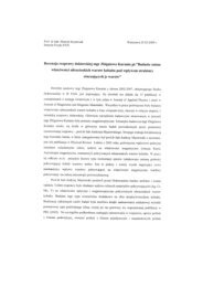
Fig. 3.2: RHEED oscillations observed during the growth of a Ga 1−x Mn x As film with x = 0.062.
The first 7 periods correspond to LT-GaAs. The "jump" in the signal occurs at the point
when the Mn shutter has been opened and the rate of oscillations increased.
GaAs was grown to a thickness in the range between 2nm -100nm. Finally, Ga 1−x Mn x As
layer in the same range of substrate temperatures to a thickness of the 105nm - 302nm was
grown. No special precaution was needed at the start of Ga 1−x Mn x As growth. However,
the properties of grown Ga 1−x Mn x As do depend on growth parameters as As overpressure
and T S . The growth was monitored in situ by reflection high energy electron diffraction
(RHEED).
The determination of Mn content in Ga 1−x Mn x As epilayers is quite difficult task. The
Mn concentration x was determined using two different methods. First, during the growth
the x values were estimated from the change in the growth rate monitored by RHEED
oscillations after the Mn shutter was opened. An example of such data is shown in Figure
3.2.
Note the rate of growth measured by RHEED oscillations is in terms of atomic layers
per second, and after the Mn shutter is opened it increases in proportion to precisely that
fraction of the Mn flux which is required to completion of atomic layers as the growth
proceeds. It is thus assumed that RHEED oscillations provide a measure of the concentration
of substitutional Mn cations Mn Ga , since only these only are required to complete
the formation of atomic layers.
And second, the Mn content was obtained from X-ray diffraction measurements by
assuming that the GaMnAs layer is fully strained by the GaAs substrate. The Mn concentration
x was calculated from measured relaxed layer lattice constant (XRD measurements

3. Samples of Pb 1−x−y−z Mn x Eu y Sn z Te and Ga 1−x Mn x As. 25
Tab. 3.3: The parameters of the LT MBE growth of GaMnAs samples - substrate temperature T S
and temperature of the Mn effusion cell T Mn , thickness of the GaMnAs layers d GaMnAs
determined from RHEED oscillations and Mn composition of investigated samples x (determined
from RHEED oscillations, X-ray diffraction and high resolution X-ray diffraction
measurements
# of the sample T S T Mn d GaMnAs x x x
[ 0 C] [ 0 C] [nm] (RHEED) (XRD) (HRXRD)
GaMnAs/GaAs
00811A 285 780 302 - 0.01 -
GaMnAs/GaAs
00119C 275 880 269 - 0.032 -
GaMnAs/GaAs
10727C 270 870 131 - 0.027 0.027
GaMnAs/GaAs
10727D 270 900 149 0.062 0.061 0.056
GaMnAs/GaAs
10727E 265 920 105 0.086 0.084 0.078
GaMnAs/GaAs
10823C 265 920 111 0.07 0.082 -
GaMnAs/GaAs
10823E 250 925 115 0.093 0.085 -
GaMnAs/GaAs
10529A 275 820 300 0.014 - -
GaMnAs/GaAs
11127A 275 - 220 0.048 - -
performed at the Notre Dame University) by use of the following equation [12]: a Lrelax
= 5.6547 + 0.0002433*x. The presence of Mn interstitials atoms as well as antisite defects
can be the reason for the observed expansion of the lattice constant of GaMnAs.
The results of high resolution X-ray diffraction measurements (HRXRD) (performed in
the Institute of Physics Polish Academy of Sciences) and the effect of Mn interstitials on
the lattice parameter of Ga 1−x Mn x As will be discussed in details in Chapter IV. In fact, a
method of determining the Mn concentration x based on the measurements of the lattice
constant a 0 in Ga 1−x Mn x As is not very reliable. The Mn concentration determined from
RHEED oscillations, the results of XRD and HRXRD and details of the growth conditions
of Ga 1−x Mn x As are collected in Table 3.3.
Additionally, the Mn concentration for the sample 10823C was confirmed by use of
systematic particle-induced X-ray emission (PIXE) measurements [13]. The PIXE measurements
revealed that sample with x determined by RHEED as 0.07 has total of Mn
content equal to 0.092. The PIXE results show the total Mn content - substitutional, interstitial,
and in the form of random precipitates (Mn inclusions) and are higher than the
values obtained from RHEED oscillations.
The Mn concentration specified in the next Chapters comes from the RHEED oscillations
measurements with the exception of three samples with the lowest Mn content for

3. Samples of Pb 1−x−y−z Mn x Eu y Sn z Te and Ga 1−x Mn x As. 26
which the change in the RHEED oscillations was too small to be reliable. In this case, i.e.
00811A, 00119C, 10727C samples the Mn content was determined only by use of X-ray
diffraction technique.

4. TRANSPORT AND MAGNETIC INVESTIGATIONS OF
FERROMAGNETIC Pb 1−x−y−z Mn x Eu y Sn z Te
4.1 Introduction
One of the purposes of the studies presented in the thesis were magnetic and transport
investigations of ferromagnetic Pb 1−x−y−z Mn x Eu y Sn z Te mixed crystals. In particular,
the influence of the presence of two types of magnetic ions incorporated into semiconductor
matrix on magnetic properties of resultant semimagnetic semiconductor is analyzed.
There are several reasons for which the semimagnetic semiconductors (SMSC’s)
based on lead chalcogenides are ideal materials for such kind of investigations. The
variety of magnetic properties occurring in IV-VI SMSC, e.g., the carrier concentration
induced paramagnet-ferromagnet and ferromagnet-spin glass transition observed in
Pb 1−x−y Mn x Sn y Te [1], [2] makes this system particularly attractive for such purposes.
The non-trivial advantage of IV-VI materials is also relative simplicity of crystal growing
and carrier concentration controlling – the latter may be achieved by means of either
doping or isothermal annealing. The magnetic properties of these compounds depend
not only on the concentration of manganese ions, but also on the density of free carriers
[14]. This behaviour is due to the combination of an RKKY type of interaction between
the magnetic ions as well as the possibility to manipulate the free carrier concentration.
The additional advantage is that for Pb 1−x−y Mn x Sn y Te crystals are very well known parameters
of crystal and energy structure. In order to simplify theoretical description of
investigated magnetic system, two types of magnetic ions were choosen with spin-only
ground state: substitutional Mn 2+ possesses S = 5/2, while Eu 2+ , the second ion in our
samples, has S = 7/2.
Practically all IV-VI semimagnetic semiconductors crystallize in rock salt crystal
structure. The lattice parameter a 0 changes linearly with the content of magnetic ions
following the Vegard law.
In general, all IV-VI semimagnetic semiconductors show metallic type of conductivity
with a very large, temperature independent, concentration of carriers. However, under
special conditions, IV-VI based semimagnetic semiconductors can exhibit insulating
properties – recently, the Eu composition induced metal-insulator transition was observed
in epitaxial layers of Pb 1−x Eu x Te [15]. Carriers are generated by metal vacancies, and
their concentration can be controlled by thermal annealing or doping. In semimagnetic
lead chalcogenides with Mn or with Eu the range of carrier concentration and the methods
to control it are quite similar to the case of appropriate IV-VI semiconductors. The presence
of even 10 at. % of Mn or Eu ions has practically no effect on carrier concentration.
Mn and Eu ions are electrically inactive in semimagnetic lead chalcogenides.
IV-VI materials are narrow gap semiconductors. Qualitatively, the electron band structure
is analogous to the band structure of non-magnetic counterpart materials. A bandstructure
model based on the consistent interpretation of transport, optical, and magnetic

4. Transport and magnetic investigations of Pb 1−x−y−z Mn x Eu y Sn z Te 28
Fig. 4.1: The band structure model of Pb 1−x−y Mn x Sn y Te mixed crystals
experimental data [16], [17], [18] is presented in Figure 4.1.
The band of electrons and the band of light holes (the presence of further L bands is
not included here) are separated by a direct band at the L point of Brillouin zone. The
energy dispertion relations of electrons and holes are nonparabolic and anisotropic. There
are four equivalent valleys of both the band of electrons and the band of light holes.
Due to the narrow energy gap the energy dispertion relation is nonparabolic and usually
described within Dimmock model [19]. The energy gap of lead chalcogenides increases
rapidly with the content increase of Mn and Eu [20], [14]. In most of IV-VI semimagnetic
semiconductors the composition dependence of other band parameters can be neglected.
An increase of the energy gap with increasing temperature is observed, similarly to lead
chalcogenides. Approximetely E Σ = 0.2 – 0.4 eV below the top of the band of light holes
there is a second valence band of heavy holes. The top of this band is located at the Σ
point of the Brillouin zone and there are 12 equivalent energy valleys of this band (Σ
band). Since the direct energy gap at the Σ point of the Brillouin zone is quite large, the
heavy hole band is expected to be parabolic. The electronic properties of p-type IV-VI
semimagnetic semiconductors with very high concentration of carriers (p ≥ 5·10 19 cm −3 )
are influenced by the presence of the band of heavy holes. The Σ band is essential for
the understanding of the correlations between magnetic and transport properties of IV-VI
semimagnetic semiconductors. The effective mass of the carriers in the Σ band is much
higher than that in the L band (m ∗ Σ ≈ 1.7m e [18], m ∗ L ≈ 0.05m e [21]).
Mn-based IV-VI semimagnetic semiconductors can be divided in two groups. The
first group consists of the materials with relatively low carrier concentration of free carriers
[22] (in the range 10 17 – 10 19 cm −3 ), for instance Pb 1−x Mn x Te. From a magnetic point
of view these materials are paramagnets above T=1K. Their magnetic behaviour closely
resambles that of the Mn containing II-VI SMSC’s and can also be attributed to antiferromagnetic
interactions of the superexchange type, although the interactions are much
weaker than in II-VI semimagnetic semiconductors. Other interspin interaction mechanisms
(e.g. direct exchange or the RKKY interaction) are expected to be negligible due

4. Transport and magnetic investigations of Pb 1−x−y−z Mn x Eu y Sn z Te 29
Fig. 4.2: Curie-Weiss temperature (Θ) versus free carrier concentration in Pb 1−x−y Mn x Sn y Te.
to the large mean interspin distances and low concentration of carriers. Below T=1K a
spin-glass phase was reported in Pb 1−x Mn x Te [23]. The second group of IV-VI SMSC’s
consists of the materials with relatively high charge carrier concentrations, of order of
10 20 – 10 21 cm −3 , e.g. Pb 1−x−y Mn x Sn y Te (with low Pb content). These compounds
exhibit a ferromagnetic phase transition at low temperatures [1]. The ferromagnetic interactions
can be explained by RKKY interactions, made effective by the high carrier
concentration and dominating over the superexchange interactions. The ferromagnetic
phase occurs once the holes start to occupy site bands with a large effective mass. The
RKKY interaction [24], [25], [26] is an indirect interaction between the magnetic ions,
which is mediated by the free charge carriers. The interaction strength can be written as:
J RKKY (R ij ) = N m∗ J 2 sd a6 0k 4 F
32π 3¯h 2 [ sin(2k F R ij ) − 2k F R ij cos(2k F R ij )
(2k F R ij ) 4 ] (4.1)
where k F is the Fermi wave number, m ∗ the effective mass of the carriers, J sd the Mn ionelectron
exchange integral, a 0 the lattice constant, N the number of valleys of the valence
band, R ij the distance between the magnetic ions.
Story et. al. [1] showed that magnetic behaviour of Pb 1−x−y Mn x Sn y Te strongly depends
on the concentration of free carriers. Figure 4.2 shows the Curie-Weiss temperature
(Θ) versus free carrier concentration as reported by Story et. al. for Pb 0.25 Mn 0.03 Sn 0.72 Te.
The nonzero Curie-Weiss temperature is proportional to the sum of all magnetic interactions
present in the material. The characteristic feature of the T c (p) dependence is
the existance of a certain threshold carrier concentration p = p t ≃ 3·10 20 cm −3 , above
which the IV-VI semimagnetic semiconductors show ferromagnetic properties. For carrier
concentration lower than the threshold value p t , the crystals exhibit paramagnetic
properties (similarly to low carrier concentration materials like PbMnTe). The observation
of concentration dependence of Curie temperature has found an interpretation within
the frames of the RKKY mechanism and the two valence band model of the band structure
of PbSnMnTe and SnMnTe [16], [17]. The strength of the RKKY interaction scales
with the effective mass of carriers. The RKKY interaction is expected to become strongly
enhanced for p ≥ p t , when the Fermi level enters the Σ band and heavy holes start to

4. Transport and magnetic investigations of Pb 1−x−y−z Mn x Eu y Sn z Te 30
participate in charge transport and in RKKY interaction. Next to the effective mass of the
carriers, the degeneracy of the valence band maxima is also important (as a prefactor of
RKKY interaction). The L band is four-fold degenerate (N L =4), whereas the Σ band is
twelve-fold degenerate (N Σ =12)
The RKKY interaction is also responsible for the magnetic behaviour of canonical
metallic spin-glasses like CuMn. Because of the high carrier concentration of carriers in
these materials (10 23 cm −3 ) the interaction rapidly oscillates between ferromagnetic and
antiferromagnetic as a function of the distance between two Mn ions. The period of this
oscillation is short compared to the average Mn-Mn distance. Due to the random position
of the Mn-ions, the interaction will be ferromagnetic or antiferromagnetic at random. This
causes a frustration of the spins resulting in a spin-glass state. The ferromagnet/spinglass
phase transition is also observed in the case of IV-VI semimagnetic semiconductors
(Pb 1−x−y Mn x Sn y Te, Sn 1−x Mn x Te) [27], [28]. This effect can be explained in frame of
RKKY interaction. For the ferromagnetism the following condition should be fullfiled:
R ≤ R 0 , where R is average interspin distance and R 0 is characteristic distance R 0 ∼
1/k F ∼ 1/p 1/3 (in this case R 0 corresponds to the first switch of the RKKY interaction
from ferromagnetic to antiferromagnetic). For R ≥ R 0 the oscillatorty character of the
RKKY interaction is expected and leads to the spin-glass order.
All Eu based IV-VI semimagnetic lead chalcogenides with low carrier concentartions
(n,p ≤ 10 19 cm −3 are paramagnetic down to about T = 1K (similarly to Mn based compounds).
The very localized character of 4f orbitals of rare earth results in very weak
exchange intreractions both between magnetic ions and between magnetic ions and free
carriers. The crystals of Sn 1−x Eu x Te are not ferromagnetic. The reason of lack of ferromagnetism
in this material is the very small sp–f exchange integral. It was experimentally
established that the J sf carrier – magnetic moment exchange constants in SnTe
with rare earths ions are related to the exchange constant for Mn ions in the following
way: Jsf Gd Mn
/Jsd
= 1/5 and Jsf Eu Mn
/Jsd
= 1/8 [29]. It results in 1/25 and 1/64 reduction of
the strength of the RKKY interaction for Gd and Eu based IV-VI SMSC’s making this
interaction negligible in these materials.
4.2 Transport characterization of Pb 1−x−y−x Mn x Eu y Sn z Te samples
All the investigated Pb 1−x−y−z Mn x Eu y Sn z Te samples were characterized by means of low
magnetic field transport measurements. The aim of the transport characterization was to
obtain information about the elementary electric properties of the investigated samples:
type as well as concentration of free carriers and their mobility. The Hall voltage V H
as well as conductivity voltage V σ were measured. In the case of IV-VI semimagnetic
semiconductors the carrier concentration is important parameter since the change of the
carrier concentration influences the magnetic behavior of the material.
The Hall bar samples with typical dimensions of 8mm × 2mm × 1mm were used for
the transport measurements. The electrical contacts were prepared always in the same
way. First the surface of the specimens was etched using the solution of Br 2 and HBr
in the proportion 1 : 20. Next, the gold contacts were deposited by use of gold chloride
water solution on the polished surface of the samples. Finally, the electrical contacts were
made using indium solder and gold wires. Typical resistance of the samples was equal to
1 mΩ. This allowed to apply relatively large current (up to 300mA). The Hall as well as

4. Transport and magnetic investigations of Pb 1−x−y−z Mn x Eu y Sn z Te 31
conductivity measurements were performed at the room and liquid nitrogen temperature.
The standard DC six probe technique at the static magnetic field up to 1T was used. All
the investigated samples occurred to be p type.
In the present thesis the nominal hole concentration was determined:
p = 1
(4.2)
eR H
where R H is the Hall constant.
The nominal value of the hole concentrations results from the value of the Hall constant
assuming that Hall coefficient r H is equal to 1. This assumption, widely applied in
the literature is not precise and the nominal Hall concentration p is very often not equal
to the real Hall concentration p 0 :
p 0 =
r H
(4.3)
eR H
where r H is the Hall scattering factor.
It is well known (see e.g. [19], [21], [30]) that the carrier transport in the IV-VI
materials is served through the two hole types: light holes p l and heavy holes p h . The
band structure model that is usually used to analyze the transport effects in PbTe, SnTe
and PbMnSnTe crystals with the high carrier concentration is schematically shown in
Figure 4.1 and described in section 1 of this Chapter. The low content of europium ions
in the studied samples (see Table 3.1) allows to assume that this model also describe band
structure of Pb 1−x−y−z Mn x Eu y Sn z Te crystals. The light hole band (L point of Brillouin
zone) is separated from the conduction band by the energy gap E 0 ∼ 300 meV. About E Σ
∼ 200meV - 400meV below the top of the valence band the heavy holes band is located
(Σ point of the Brillouin zone).
Two-carrier transport is the reason for the discrepancy between the calculated nominal
hole concentration (by use of Equation 4.2) and the real value of hole concentration in
the investigated samples. In the case of the carrier transport via light and heavy holes,
Hall constant is the function of both light and heavy holes carrier concentration, mobility
and Hall scattering factor:
R H = p le l r l µ 2 l + p he h r h µ 2 h
(p l e l µ l + p h e h µ h ) 2 (4.4)
where p l , p h - light and heavy hole concentration e l , e h - electric charge of carriers r l , r h -
Hall scattering factors of carriers µ l , µ h - mobilities of carriers.
If both the light and heavy holes carry the same elementary charge (+e), Equation 4.4
has the following form:
R H = r lp l + b 2 p h r h
e(p l + bp h ) 2 (4.5)
where b = µ h /µ l .
The Hall scattering factors r l and r h in the Equation 4.4 depend on both statistical
energy distribution of carriers and band structure anisotropy:
r H = r τ r a (4.6)
where r τ - standard Hall factor that takes into consideration statistical energy distribution
of carriers r a - term related to the anisotropy.

4. Transport and magnetic investigations of Pb 1−x−y−z Mn x Eu y Sn z Te 32
In the strong degenerate systems energy of carriers that participate in transport is equal
to Fermi energy (delta type of statistical energy distribution) and r τ =1. For the materials
with anisotropic effective mass or anisotropic time relaxation:
where
r a =
3K(K + 2)
(2K + 1) 2 (4.7)
K = (m ‖ /m ⊥ )(τ ⊥ /τ ‖ ) (4.8)
Anisotropic contribution to the Hall factor (r a ) decreases from r a =1 for K=1 to r a =0.75
for K≫1.
The real hole concentration in the sample can be determined by use of the following
equation:
p 0 = r ∗ Hp (4.9)
where
rH ∗ = (p lr l + b 2 p h )(p l + p h )
(4.10)
(p l + bp h ) 2
and
p 0 = p l +p h - real hole concentration in the sample
p = 1/(e R H ) - nominal hole concentration
b = µ h /µ l - heavy hole mobility to light hole mobility ratio
p l , p h - light and heavy hole concentration
r l = 3K(K+2)/(2K+1) 2 - Hall scattering factor for light holes, K = 10 - anisotropy coefficient
for light hole band.
To determine r ∗ H coefficient, that is function of hole concentration in the sample, one
needs to know the light as well as heavy hole concentration and ratio of their mobilities.
In the present thesis only nominal Hall concentration was determined at the room
and liquid nitrogen temperature and all experimental data are shown as a function of
nominal concentration (p). The nominal Hall concentration is commonly used in the
characterization of IV-VI compounds and is unambiguous experimental parameter.
All the investigated samples occurred to be p type with the high almost temperature
independent hole concentration (in the range between 2·10 18 cm −3 and 2·10 21 cm −3 ).
The obtained values of hole concentration, conductivity and mobility measured at the
room and nitrogen temperature are shown in Table 4.1. Typical values of the Hall voltage
were equal from several to several dozen microvolts. Simultaneously, the large values
of the asymmetry voltage (resulting from non equipotential positions of the Hall probes),
exceeding 100µV were observed. The asymmetry voltage as well as influence of the magnetoresistance
on the Hall effect was eliminated by the standard averaging procedure of
results obtained for the combination of two current as well as magnetic field polarizations.
Additionally, using of the Keithley 150B voltometer allowed to reset the asymmetry voltage
at the magnetic field equal to zero. The values of carrier concentration, conductivity
and mobility were determined with the uncertainty of 15 percent at the room temperature
and 30 percent at the liquid nitrogen temperature. One of the investigated samples 809 − 30
was isothermally annealed, to increase hole concentration. The procedure of annealing
performed at the telluride atmosphere and temperature of 700 0 C for 48 hours allowed to
increase hole concentration from 4.22·10 20 cm −3 to 8.25 10 25 cm −3 . The surface of the
sample was polished after annealing.

4. Transport and magnetic investigations of Pb 1−x−y−z Mn x Eu y Sn z Te 33
Tab. 4.1: The results of transport characterization of Pb 1−x−y−z Mn x Eu y Sn z Te samples - hole concentration
p [10 21 cm −3 ], conductivity σ[(Ωcm) −1 ], mobility µ [cm 2 /Vs]) measured at
the room and liquid nitrogen temperature.
sample x P b x Mn x Eu x Sn p σ µ p σ µ
number 300K 300K 300K 77K 77K 77K
841_14 - 0.116 0.011 0.873 1.40 3554 15.8 0.93 3029 20.7
841_18 - 0.131 0.134 0.735 1.30 3683 15.5 1.04 5598 33.3
842_4 - 0.063 0.0045 0.932 1.40 1172 5.2 - - -
842_8 - 0.068 0.003 0.929 1.56 3500 14.0 - - -
842_14 - 0.070 0.007 0.923 1.56 1933 7.7 1.25 2750 13.7
842_20 - 0.091 0.009 0.9 1.21 3480 17.9 1.16 4561 24.6
848_4 - 0.061 0.0115 0.927 1.77 4533 16.0 1.70 6648 24.7
848_10 - 0.064 0.012 0.924 1.93 1696 5.5 - - -
848_16 - 0.050 0.011 0.939 1.24 6435 32.3 1.48 9635 40.60
848_22 - 0.065 0.018 0.917 1.37 3557 16.2 - - -
848_24 - 0.051 0.019 0.93 1.57 3216 17.4 1.29 4842 23.5
848_26 - 0.074 0.023 0.903 1.66 6370 23.9 - - -
809_2 0.116 0.031 0.0027 0.85 1.01 5860 29 1.01 19050 76
809_4 0.118 0.030 0.0016 0.85 0.501 4050 48.6 0.657 596 30
809_10 0.187 0.030 0.0031 0.78 0.601 2920 29 3.0 4983 35
809_12 0.215 0.022 0.003 0.76 0.401 3390 49 0.60 6764 69
809_30 0.256 0.024 0.010 0.71 0.425 1310 19.2 0.762 2058 16.9
809_30 0.256 0.024 0.010 0.71 0.822 3346 25.4 1.04 5307 31.8
anneal.
809_32 0.27 0.026 0.014 0.69 0.325 2777 53.5 0.49 4731 35.2
809_34 0.276 0.027 0.017 0.68 0.449 2970 41.4 0.98 2373 15.2
809_36 0.272 0.025 0.013 0.69 0.318 2823 55.4 0.75 4816 40
793_2 0.990 0.010 0.000 - 0.002 202 540 0.003 1502 2641
793_4 0.989 0.010 0.001 - 0.003 112 263 0.004 807 1399
793_6 0.982 0.009 0.009 - 0.002 72 75 0.003 723 1329
793_10 0.910 0.005 0.004 - 0.005 11 14 - - -
793_12 0.990 0.007 0.003 - 0.005 1910 24.5 0.007 3076 24.4

4. Transport and magnetic investigations of Pb 1−x−y−z Mn x Eu y Sn z Te 34
4.3 Magnetic measurements of Pb 1−x−y−z Mn x Eu y Sn z Te mixed crystals
In the present section the results of magnetic studies of Pb 1−x−y−z Mn x Eu y Sn z Te samples
will be presented. As was shown in the previous section all the investigated samples occured
to be p-type with practically temperature independent concentration of carriers.
Two groups of IV-VI semimagnetic semiconductors with two types of magnetic ions
(Mn 2+ and Eu 2+ ) were investigated. First, the samples of Pb 1−x−y Mn x Eu y Te (0.005≤
x ≤0.010, 0≤ y ≤0.009) with relatively low free carrier concentration (2.30·10 18 cm −3
≤ p ≤ 4.80·10 20 cm −3 at T=300K) were studied. Next, the second group of samples:
Pb 1−x−y−z Mn x Eu y Sn z Te (0.022 ≤ x ≤0.031, 0.002 ≤ y ≤0.017, 0.0680 ≤ z ≤0.850 )
as well as Sn 1−x−y Mn x Eu y Te (0.055 ≤ x ≤0.131, 0.003 ≤ y ≤0.023), characterized by
substantially larger carrier concentration (3.20·10 20 cm −3 ≤ p ≤ 1.01·10 21 cm −3 , 1.21
10 21 cm −3 ≤ p ≤ 1.93·10 21 cm −3 for Pb 1−x−y−z Mn x Eu y Sn z Te and Sn 1−x−y Mn x Eu y Te,
respectively at T=300K) was investigated.
AC magnetic susceptibility studies in the temperature range 1.3-150 K using a mutual
inductance method as well as DC magnetization measurements in the magnetic field range
0-90 kOe (0-9 T) at various temperatures by use of extraction technique were carried out.
The susceptibility measurements were carried out in AC magnetic field of frequency in
the range 7-10000 Hz and amplitude not exceeding 5 Oe (5·10 −4 T).
Generally, in the range of high temperatures all IV-VI semimagnetic semiconductors
are Curie-Weiss paramagnets with the temperature dependence of the magnetic susceptibility
described by the Curie-Weiss law:
χ(T ) = C/(T − Θ) (4.11)
where C = g 2 µ 2 B S(S + 1)N M is the Curie constant and k B Θ = 1/3S(S + 1)x ∑ z i I(R i )
is the paramagnetic Curie temperature (Curie-Weiss temperature). Here, N M is the concentration
of magnetic ions, z i is the number of magnetic neighbors on i–th crystalographic
shell, I(R i ) is the exchange integral between the central ion and its i–th magnetic
neighbors, S is the spin of the magnetic ion, g is the spin-splitting g factor, k B is the
Boltzman constant, µ B is the Bohr magneton.
For all the investigated samples the high temperature behaviour of the inverse lowfield
susceptibility χ −1 was nearly linear and all data were fitted with Curie-Weiss law of
the form 1 :
χ(T ) = C/(T − Θ) + χ dia (4.12)
where χ dia is the susceptibility of the host lattice (all IV-VI semiconductors without magnetic
ions are standard diamagnetic materials with magnetic susceptibility around χ dia
≃ -3·10 −7 emu/g). Figure 4.3 presents the high temperature behaviour of inverse magnetic
susceptibility for a few Pb 1−x−y Mn x Eu y Te samples. The determined values of paramagnetic
Curie temperature Θ, which is proportional to the total strength of exchange
interactions between magnetic ions and Curie constant C are presented in Table 4.2.
In the case of PbMnEuTe obtained results (the determined negative and relatively
small values of paramagnetic Curie-Weiss temperature Θ) indicate that weak antiferromagnetic
superexchange interaction occurs the dominant mechanism in PbMnEuTe crystals.
The obtained results correspond to those reported in PbMnTe. Inspection of Table
1 The Curie-Weiss law in the form of equation 4.12 describes system with one type of magnetic ions,
i.e. PbSnMnTe.

4. Transport and magnetic investigations of Pb 1−x−y−z Mn x Eu y Sn z Te 35
Tab. 4.2: . The results of magnetic measurements for IV-VI mixed crystals.
sample x P b x y z C Θ T C T f
number [emu/g] [K] [K] [K]
841_14 - 0.116 0.011 0.873 0.00215 19.65 17.46 -
841_18 - 0.131 0.013 0.856 0.00209 18.18 16.63 -
842_4 - 0.063 0.0045 0.932 - - 10.90 -
842_8 - 0.068 0.003 0.929 - - 13.07 -
842_14 - 0.070 0.007 0.923 - - 15.23 -
842_20 - 0.091 0.009 0.900 0.00230 17.98 17.10 -
848_4 - 0.061 0.0115 0.927 0.00141 11.57 11.57 -
848_10 - 0.064 0.012 0.924 - - 8.35 -
848_16 - 0.050 0.011 0.939 0.00149 11.02 8.75 -
848_22 - 0.065 0.018 0.917 - - 10.75 -
848_24 - 0.051 0.019 0.930 0.00222 12.08 10.98 -
848_26 - 0.074 0.023 0.903 - - 11.31 -
809_2 0.116 0.031 0.003 0.850 0.00047 5.16 - 2.0
(Re(χ)
625Hz)
809_4 0.118 0.030 0.002 0.850 0.00050 4.88 - -
809_10 0.187 0.030 0.003 0.780 0.00050 4.74 4.13 -
809_12 0.215 0.022 0.003 0.760 0.00052 4.55 4.09 -
809_30 0.256 0.024 0.010 0.710 0.00080 3.02 2.98 -
809_30 0.256 0.024 0.010 0.710 0.00080 4.16 3.55 -
anneal.
809_32 0.27 0.026 0.014 0.690 0.00082 2.89 2.81 -
809_34 0.276 0.027 0.017 0.680 0.00090 2.60 2.60 -
809_36 0.272 0.025 0.013 0.690 0.00077 3.13 3.12 -
793_2 0.99 0.010 0.000 - 0.00039 -0.93 - -
793_4 0.989 0.010 0.001 - 0.00038 -0.69 - -
793_4 0.989 0.010 0.001 - 0.00038 -0.69 - -
793_6 0.982 0.009 0.009 - 0.00051 -1.12 - -
793_10 0.991 0.005 0.004 - 0.00053 -0.42 - -
793_12 0.99 0.007 0.003 - 0.00059 -0.39 - -
793_14 0.99 0.005 0.005 - 0.00086 -0.41 - -

4. Transport and magnetic investigations of Pb 1−x−y−z Mn x Eu y Sn z Te 36
4.2 shows that no distinct trends in Θ and C dependence on Eu concentration can be observed.
However, it should be stressed that the values analyzed are determined with rather
large error related with considerable uncertainty of chemical compositions of the samples.
Figures 4.4 and 4.5 present high temperature part of inverse AC susceptibility for
several PbMnEuSnTe and SnMnEuTe samples. The fitting procedure (the Curie–Weiss
law – the same as for PbMnEuTe samples) revealed the positive values of Curie–Weiss
temperature in this group of IV-VI mixed crystals. This indicates the presence of ferromagnetic
interactions. The obtained values of Curie–Weiss temperature Θ and Curie
constant C are shown in Table 4.2.
χ
Fig. 4.3: Inverse AC susceptibility versus temperature measured for Pb 1−x−y Mn x Eu y Te samples
(793 − 2: x=0.010, y=0; 793 − 4: x=0.010, y=0.001; 793 − 10: x=0.005, y=0.004; 793 − 12:
x=0.007, y=0.003; 793 − 14: x=0.005, y=0.005). The solid lines correspond to Curie -
Weiss law fits.
The careful inspection of Table 4.2 allows to notice significant changes of Curie-
Weiss temperature with the Eu content. The decrease of the paramagnetic Curie temperature
Θ with the increase of Eu concentration is clearly visible. The three samples of
Pb 1−x−y−z Mn x Eu y Sn z Te: 809 − 12, 809 − 30, 809 − 34 are characterized with very similar
values of Mn content and concentration of free holes (see Table 4.1). For the Mn concentration
equal to around x ≃ 0.02 and free hole concentration p ≃ 4 10 20 cm −3 increase
of Eu content from y=0.003 to y=0.01 leads to the decrease of Curie–Weiss temperature
from 4.55K to 3.02K and for y=0.017 paramagnetic Curie temperature is equal to 2.63K.
In the case of Sn 1−x−y Mn x Eu y Te crystals such distinct tendency is not observed (see Table
4.2). However, one needs to realize that obtained values of chemical composition as
well as free carrier concentration are determined with quite large uncertainty.
The low temperature studies revealed the presence of paramagnet/ferromagnet phase
transition in the case of SnMnEuTe as well as the most of PbSnMnEuTe samples. Figures
4.6 and 4.7 show the low temperature behaviour of real component of AC susceptibility
Re(χ) for several samples of studied Pb 1−x−y−z Mn x Eu y Sn z Te and Sn 1−x−y Mn x Eu y Te
mixed crystals. Typical behaviour of a ferromagnet is observed. Both components of the
susceptibility dramatically increase at the Curie temperature T C . The Curie temperature

4. Transport and magnetic investigations of Pb 1−x−y−z Mn x Eu y Sn z Te 37
χ
Fig. 4.4: The high temperature inverse AC susceptibility measured for several
Pb 1−x−y−z Mn x Eu y Sn z Te samples (809 − 2: x=0.031, y=0.003, z=0.850; 809 − 12:
x=0.022, y=0.003, z=0.760; 809 − 32: x=0.026, y=0.014, z=0.69; 809 − 34: x=0.027,
y=0.017, z=0.680).The solid lines correspond to Curie -Weiss law fits.
was determined by the maximum slope of dRe(χ) . The obtained values of T
dT
C are shown
in Table 4.2. T C values are approximately equal to the Curie-Weiss temperature Θ determined
from high temperature susceptibility measurements. The low temperature measurements
confirmed the described above tendency for studied Pb 1−x−y−z Mn x Eu y Sn z Te
crystals, i.e. the decrease of Curie temperature with the Eu content.
Additionally performed DC magnetization measurements (up to 9T at various temperatures)
collaborate susceptibility investigations and confirm ferromagnetic ordering
observed for most of PbSnMnEuTe samples. Figure 4.8 presents an example of performed
magnetization studies for 809 − 10 (x=0.030, y=0.003, z=0.78) ferromagnetic sample sample
with p=6·10 20 cm −3 .
For the sample of PbSnMnEuTe (809 − 2) the ferromagnetic to spin glass phase transition
is observed. Figure 4.9 presents characteristic behaviour of low temperature part
of real as well as imaginary component of susceptibility for spin glass (809 − 2) as well
as ferromagnetic (809 − 12) samples of Pb 1−x−y−z Mn x Eu y Sn z Te. In the case of ferromagnetic
sample (with the concentration of free holes equal to 4.0·10 20 cm −3 ) the sharp
transitions in both real and imaginary components of susceptibility occur. For spin glass
sample (characterized by higher free hole concentration p=1·10 21 cm −3 ) a cusp in Re(χ)
is visible at the freezing temperature T f . The magnitude of the susceptibility at this cusp
is much lower than the susceptibility of the ferromagnetic sample. A corresponding maximum
in the out of phase of susceptibility Im(χ) is observed at slightly lower temperature.
The 809 − 2 PbMnEuSnTe sample shows an obvious characteristics of spin glass–like
phase. The cusp observed in susceptibility χ versus temperature T shifts to higher temperatures
when the frequency f of the applied AC field is increased. This feature – the
increase of the freezing temperature when the frequency is higher – was observed in the

4. Transport and magnetic investigations of Pb 1−x−y−z Mn x Eu y Sn z Te 38
χ
Fig. 4.5: The high temperature inverse AC susceptibility measured for several Sn 1−x−y Mn x Eu y Te
samples (841 − 18: x=0.131, y=0.013; 841 − 14: x=0.116, y=0.011; 842 − 20: x=0.091,
y=0.009; 848 − 4: x=0.061, y=0.0115; 848 − 16: x=0.050, y=0.011; 848 − 24: x=0.051,
y=0.019).
well-known canonical spin glass systems [31], [32], [33], [34]. The increase of T f per
decade of frequency is approximately constant and frequency dependence occurs in both
real and imaginary part of AC magnetic susceptibility. Figures 4.10 and 4.11 present the
frequency dependence of low temperature parts of real and imaginary components of susceptibility
for 809 − 2 sample of PbMnEuSnTe. The relative shift of freezing temperature
T f per decade of frequency R = ∆T f /T f ∆logf is equal to 0.021. The rate of the changes
corresponding to maximum in imaginary part of susceptibility is higher: R=0.048.
The values of R reported for known spin glass systems range from 0.005 (Cu) to
0.11 (La 1−x Gd x Al 2 [35]) and the rate of the change in Im(χ) is the same as the rate of
the change in Re(χ). The values of R reported for Sn 1−x Mn x Te are equal: R=0.027
(x=0.04) [27], R=0.022 (x=0.008) [36], R=0.027 (x=0.022) [36]. It appears that in
the case of Sn 1−x Mn x Te mixed crystals the character of the spin glass phase does not
depend on the manganese concentration. In the case of studied in the present thesis
Pb 1−x−y−z Mn x Eu y Sn z Te mixed crystals, comparable with Mn-based IV-VI semimagnetic
semiconductors, the significant difference is visible in the inequality of frequency shift in
Re(χ) and Im(χ). It has to be noted that Im(χ) in conducting media is distorted because
of the eddy currents induced by AC magnetic field. Nevertheless, obtained values differ
from those obtained for analogous materials (Sn 1−x Mn x Te), in particular the difference
in the rate of frequency shift of cusp in real and imaginary part of susceptibility seems to
be significant.
Figure 4.12 presents magnetic phase diagram for PbMnSnTe and PbMnEuSnTe samples.
The magnetic phase diagram for PbMnSnTe mixed crystals was taken from the Ref.
[27] and data for PbMnEuSnTe samples studied in the present thesis were included.
The magnetic phase of the samples at low temperatures is indicated as a function
of both: manganese concentration and free hole concentration. Three regimes can be

4. Transport and magnetic investigations of Pb 1−x−y−z Mn x Eu y Sn z Te 39
χ
!"#$"%
Fig. 4.6: The low temperature behaviour of real part of susceptibility for several
Pb 1−x−y−z Mn x Eu y Sn z Te samples (809 − 12: x=0.022, y=0.003, z=0.760; 809 − 36:
x=0.025, y=0.013, z=0.690; 809 − 30: x=0.024, y=0.010, z=0.710 ;809 − 32: x=0.026,
y=0.014, z=0.690; 809 − 34: x=0.027, y=0.017, z=0.680).
distinguished: a ferromagnetic regime for high manganese and high carrier concentration;
a spin glass regime for low manganese and high carrier concentrations; and a reentrant
spin glass regime separating the former two. A sample is considered as a reentrant spin
glass if in the temperature range two transitions can be observed (ferromagnetic as well
as spin glass). It is clearly visible that the presence of Eu shifts spin glass regime towards
lower carrier concentration p. In the case of Sn 1−x Mn x Te any changes after introducing
Eu to semiconductor matrix are not observed in magnetic phase diagram.
The most likely reason of the strong dependence of Curie temperature on Eu content is
a variation of the band parameters with the alloy composition. In the qualitative analysis
of the above problem the following points should be considered.
• The Eu atom is a magnetic impurity in PbMnSnTe matrix with spin-only ground
state: Eu 2+ has S =7/2. The electrons of the half-filled f-shell, responsible for the
magnetic Eu moment, are very weakly coupled to the band electrons. Thus, one can
not expect a substantial contribution of Eu magnetic ions to average magnetization.
The coupling constant J s−f is much smaller than J s−d constant. However there
exists a small contribution to the total energy from s–f coupling between Eu atoms
and carriers. One can expect an increase of Curie temperature with the Eu content
from this mechanism. Since the experiment shows the opposite behaviour, it can be
assumed that the role of Eu as a magnetic impurity is negligible.
• Since EuTe is an antiferromagnet, one can expect a transition from positive (Curie)
to negative (Neel) temperature of magnetic ordering of PbMnEuSnTe when changing
Eu content y from 0 to 1. For small Eu content it can lead to a decrease of
T C .

4. Transport and magnetic investigations of Pb 1−x−y−z Mn x Eu y Sn z Te 40
χ
!
Fig. 4.7: The low temperature behaviour of real part of susceptibility for several
Sn 1−x−y Mn x Eu y Te samples (841 − 14: x=0.121, y=0.011; 842 − 20: x=0.090, y=0.009;
841 − 18: x=0.128, y=0.014; 848 − 24: x=0.055, y=0.0175; 848 − 16: x=0.054, y=0.011;
848 − 4: x=0.058, y=0.011).
• Eu is a component of the complex PbMnEuSnTe alloy and one should consider a
variation of the band parameters as a function of Eu content. For the qualitative
analysis, let’s assume here a simplified two-band model with some phenomenological
parameters. It should be stressed that the real spectrum of IV-VI compounds
is rather complicated and one should account for nonparabolicity and anisotropy of
energy bands.
For a qualitative analysis, the following formula describing RKKY interaction strength
can be used:
J RKKY (R ij ) = N m∗ Jsd 2 a6 0kF
4 sin(2k F R ij ) − 2k F R ij cos(2k F R ij )
32π 3¯h 2 (4.13)
(2k F R ij ) 4
where k F is the Fermi wave number, m ∗ the effective mass of the carriers, J sd the Mn ionelectron
exchange integral, a 0 the lattice constant, N the number of valleys of the valence
band, R ij the distance between the magnetic ions.
If one will take R ij equal to the mean distance between the magnetic ions (Mn) R
this formula will give the mean interaction energy between magnetic impurities which is
roughly equal to the transition temperature T C ≈ J RKKY (R)/k B . It should be stressed
here, that Equation 4.13 was obtained for a parabolic energy spectrum and does not take
into account the anisotropy.
It is assumed that the hole energy spectrum in L points has the form:
and, respectively, in Σ points:
E L (k) = (∆ 2 + v 2 k 2 ) 1/2 (4.14)
E Σ (k) = ɛ 0 + ¯h2 k 2
2m ∗ Σ
(4.15)

4. Transport and magnetic investigations of Pb 1−x−y−z Mn x Eu y Sn z Te 41
0.3
PbSnMnEuTe 809_10
M [emu/g]
0.2
0.1
4.3K
12K
30K
0.0
0 2 4 6 8 10
B [T]
Fig. 4.8: Magnetization measured at various temperatures and magnetic fields up to 9T for
Pb 1−x−y−z Mn x Eu y Sn z Te 809 − 10 sample with x=0.030, y=0.003, z=0.780 and hole
concentration p=6 10 20 cm −3 .
Here, v is band-coupling constant and it is assumed that v=5 10 −8 eV [37], ∆ = E g /2
and ɛ 0 parameters depend on alloy composition, m ∗ Σ = 3m 0, m 0 is free electron mass.
It is commonly known that the energy spectrum of Pb 1−y Eu y Te alloy is very sensitive
to the concentration of Eu. The energy gap E g depends strongly on Eu content - from
189.7 meV for y=0 (PbTe) to 248 meV for y=0.013 at the temperature T =10K [37],
dE g /dy=5.788 eV at T =10K for y

4. Transport and magnetic investigations of Pb 1−x−y−z Mn x Eu y Sn z Te 42
χχ !"
χ
χ
χ
χ
#$%&$'"
Fig. 4.9: The low temperature behaviour of both real Re(χ) and imaginary Im(χ) component of
susceptibility for two samples of Pb 1−x−y−z Mn x Eu y Sn z Te: 809 − 2 (x=0.031, y=0.003,
p=1·10 21 cm −3 ) and 809 − 12 (x=0.022, y=0.003, p=4·10 20 cm −3 ). The typical ferromagnetic
characteristics is observed for 809 − 12 sample and spin glass behaviour for the
sample with higher free hole concentration.
which gives the total hole concentration p 0 and takes into account the degeneracy of each
valley. It is accepted here that p 0 is equal to 4·10 20 cm −3 .
The Fermi momentum in the Σ band kF Σ = (2m∗ Σ (E F − ɛ 0 )) 3/2 can be found as a solution
of Equation 4.20. Next, Equation 4.13 with k F = kF Σ, R = ( 3a3 0
4πx )1/3 , a 0 =6.5·10 −8
cm, N=12, J sd =1 eV is used for T C calculations. The obtained T C dependence on Eu concentration
y for various values of Sn content (0.6 ≤ z ≤ 1) is shown in Figure 4.13. It is
clearly visible that the obtained results of calculations performed within simple two band
model can explain the observed experimentally tendency of Curie temperature decrease
with Eu content. The obtained values of Curie temperature are higher than determined
experimentally. However, it should be stressed that not all phenomenological parameters
were known precisely. Many assumptions are introduced to the model. Nevertheless, the
calculated dependence of Curie temperature on Eu content very well reflects experimentally
confirmed effect of the T C decrease with Eu concentration y.
Since the effect of the decrease of Curie temperature with the increase of Eu content
due to change of band parameters is pronounced in PbSnMnEuTe mixed crystals, one
should observe the change of T C under hydrostatic pressure.
Magnetization measurements under hydrostatic pressure up to 12 kbar were performed
in the temperature above 4.2K and magnetic fields up to 16 kOe (1.6 T) using
the vibrating sample magnetometer. A miniature CuBe container with the inner diameter
of 1.42 mm was used as a pressure cell and a mixture of mineral oil and kerosene
was used as a pressure-transmitting medium. The pressure at low temperatures was determined
using the pressure dependence of the superconducting transition temperature
for the pure Sn probe placed near the sample. The experimental setup allows to per-

4. Transport and magnetic investigations of Pb 1−x−y−z Mn x Eu y Sn z Te 43
χ
!" #
Fig. 4.10: The frequency dependence of real component of susceptibility Re(χ) for the sample
of Pb 1−x−y−z Mn x Eu y Sn z Te: 809 − 2: x=0.031, y=0.003, p=1·10 21 cm −3 . The shift of
the freezing temperature T f towards higher temperatures with the frequency increase is
clearly visible.
form magnetization studies under hydrostatic pressure in the temperatures above T =4.2
K. Thus, it was possible to investigate only Sn 1−x−y Mn x Eu y Te samples with Curie temperatures
higher than 4.2K. Unfortunately, all available Pb 1−x−y−z Mn x Eu y Sn z Te samples
were characterized by lower than 4.2K Curie temperature. Two samples were measured:
one of Sn 1−x−y Mn x Eu y Te (842 − 8 with x=0.068, y=0.003, p=1.6·10 21 cm −3 ) and one of
Sn 1−x Mn x Te (x=0.10). Figures 4.14 and 4.15 show the results of zero field cooled (ZFC)
low-field magnetization, measured at ambient and equal to 11.2 kbar pressure for SnMnEuTe
and 10.5 kbar for SnMnTe sample. In both cases the decrease of Curie temperature
under hydrostatic pressure is observed. T C shifts towards low temperatures with the same
pressure coefficient for two investigated samples: dT C
∼ -0.03 K/kbar.
dP
The ZFC magnetization measurements performed as a function of magnetic field up
to 16 kOe (1.6T) at low temperatures (presented in Figures 4.16 and 4.17) revealed
the decrease of spontaneous magnetization in both cases with almost the same pressure
coefficient: dM 0
∼ -0.026 emu/g kbar for SnMnEuTe sample and dM 0
∼ -0.03 emu/g kbar
dP dP
for SnMnTe sample. There is no pressure effect on the coercive field of the hysteresis
loops measured for both SnMnEuTe as well as SnMnTe samples.
In fact, performed magnetization measurements under hydrostatic pressure revealed
that introducing Eu ions into semiconductor matrix of SnMnTe does not influence significantly
Curie temperature. However, the magnetic studies of SnMnEuTe mixed crystals
with much higher concentration of Eu are needed to form the final conclusions.
The effect of T C dependence on hydrostatic pressure is well known in PbMnSnTe
semimagnetic semiconductor. T. Story [10] observed three different regions of the Curie
temperature variation with the pressure - corresponding to three various pressure coefficients
dT C
dP . For the Pb 1−x−yMn x Sn y Te samples with low free carrier concentration (about
3·10 20 cm −3 ) very significant increase of Curie temperature (approximately 100%) after
applying the hydrostatic pressure equal to 10kbar is observed. Next, the samples with
slightly higher free carrier concentration (6-7·10 20 cm −3 ) reveal no effect in the pressure

4. Transport and magnetic investigations of Pb 1−x−y−z Mn x Eu y Sn z Te 44
χ
!" #
Fig. 4.11: The frequency dependence of imaginary part of susceptibility Im(χ) for the sample of
Pb 1−x−y−z Mn x Eu y Sn z Te: 809 − 2 (x=0.031, y=0.003, p=1·10 21 cm −3 ). The maximum
of the observed cusp shifts towards higher temperatures with the frequency increase.
dependence of Curie temperature – in this case the values of dT C
are equal to zero. At
dP
least, for the samples with high carrier concentration p=1·10 21 cm −3 the decrease of T C
with the pressure increase is observed ( negative values of dT C
coefficient). Simultaneously,
transport investigations [10] revealed that hydrostatic pressure does not change the
dP
total free hole concentration, but significantly changes distribution of carriers between
light hole (L) and heavy hole (Σ) bands. The experimental results showed that pressure
coefficient dT C /dP (p) dependence reflects the threshold behaviour of T C as a function of
hole concentration p. It is presented [10] that for PbSnMnTe mixed crystals energy gap
increases with the hydrostatic pressure dE g /dP =8meV/kbar and ɛ 0 energy decreases with
hydrostatic pressure dɛ 0 /dP =-4meV/kbar. T. Story showed [10] that hydrostatic pressure
induces the changes in the band parameters of PbSnMnTe mixed crystals and this in turn
leads to the observed changes in Curie temperature.

4. Transport and magnetic investigations of Pb 1−x−y−z Mn x Eu y Sn z Te 45
Fig. 4.12: Magnetic phase diagram for Pb 1−x−y Mn x Sn y Te [27] and Pb 1−x−y−z Mn x Eu y Sn z Te
samples. Red triangles correspond to PbMnEuSnTe ferromagnets, red circles to PbMnEuSnTe
spin glasses, black circles to PbMnSnTe ferromagnets, green circles to PbMn-
SnTe spin glasses, blue circles to reentrant spin glasses. Lines present model calculations
of the phase boundary (see Ref. [27]): solid line presents geometric model, dashed
and dot dashed lines correspond to Sherrington-Kirkpatrick model, dot line correspond
to Sherrington-Southern model
8
Curie Temperature [K]
7
6
z=1
z=0.9
z=0.8
z=0.7
z=0.6
5
0,000 0,005 0,010 0,015
Eu content y
Fig. 4.13: Curie temperature calculated for Pb 1−x−y−z Mn x Eu y Sn z Te mixed crystals as a function
of Eu content y for various values of Sn concentration 0.6 ≤ z ≤ 1 and Mn concentration
x=0.02

4. Transport and magnetic investigations of Pb 1−x−y−z Mn x Eu y Sn z Te 46
0.7
0.6
SnMnEuTe 842_8
P=0
P=11.2 kbar
0.5
ZFC
B=20 Oe
M [emu/g]
0.4
0.3
0.2
∆T C
/dP ~ - 0.03 K/kbar
0.1
0.0
4 6 8 10 12 14 16 18 20 22 24 26
T [K]
Fig. 4.14: Zero field cooled magnetization measured as a function of temperature for
Sn 1−x−y Mn x Eu y Te sample (842 − 8 with x=0.068, y=0.003, p=1.6·10 21 cm −3 ) at ambient
and equal to 11.2 kbar pressure.
0.8
0.7
SnMnTe
x=0.10
M [emu/g]
0.6
0.5
0.4
0.3
∆T C
/dP ~ - 0.03 K/kbar
P=0
10.5 kbar
ZFC
B=20 Oe
0.2
0.1
0.0
2 4 6 8 10 12 14 16 18 20 22 24 26
T [K]
Fig. 4.15: Zero field cooled magnetization measured as a function of temperature for Sn 1−x Mn x Te
sample with x=0.10 at ambient and equal to 10.5 kbar pressure.

4. Transport and magnetic investigations of Pb 1−x−y−z Mn x Eu y Sn z Te 47
10
8
6
4
SnMnEuTe 842_8
P=0
P=11.2 kbar
M 0
M [emu/g]
2
0
-2
ZFC
T=5 K
∆M 0
/dP ~ - 0.026 emu/g/kbar
-4
-6
-8
-10
-18 -16 -14 -12 -10 -8 -6 -4 -2 0 2 4 6 8 10 12 14 16 18
B [kOe]
Fig. 4.16: Zero field cooled magnetization measured as a function of magnetic field at low temperature
T =5K for Sn 1−x−y Mn x Eu y Te sample (842 − 8 with x=0.068, y=0.003, p=1.6·10 21
cm −3 ) at ambient and equal to 11.2 kbar pressure.
8
M [emu/g]
6
4
M 0
∆M 0
/dP ~ - 0.03 emu/g/kbar
P=0
10.5 kbar
SnMnTe
x=0.10
ZFC
T=4.2 K
2
0
0 2 4 6 8 10 12 14 16
B [kOe]
Fig. 4.17: Zero field cooled magnetization measured as a function of magnetic field at low temperature
T =4.2K for Sn 1−x Mn x Te sample with x=0.10 at ambient and equal to 10.5 kbar
pressure.

5. LOW TEMPERATURE ANNEALING STUDIES OF Ga 1−x Mn x As
5.1 Introduction
In this chapter the results of experimental studies of low temperature (LT) Ga 1−x Mn x As
will be presented. Ga 1−x Mn x As has become the focus of current interest because of its
high Curie temperature and possible spin-electronics applications (see [38] and references
therein). One of the issues investigated in the presented thesis was the effect of the low
temperature (LT) annealing on the electronic, magnetic and structural properties of the
Ga 1−x Mn x As. The purpose of this work was to systematically anneal and study the samples
over a wide range of Mn concentration. The role of Mn interstitial in GaMnAs is
explored. The as-grown as well as annealed samples were systematically investigated.
This introduction includes briefly review of the physical properties reported for LT
Ga 1−x Mn x As epilayers. Ga 1−x Mn x As is the subject of very intense interest, since it became
a favorite material for spintronics. Many papers present in the literature force to
give very brief and selective survey of the reported results.
Typically, the GaMnAs is grown by use of low temperature molecular beam epitaxy
(LT MBE, growth temperature

5. Low temperature annealing studies of Ga 1−x Mn x As 49
and x, it has not been really understood. Particularly, the results of high resolution X-ray
diffraction (HRXRD) presented in this thesis show that Mn interstitials are responsible for
the observed expansion of the lattice constant. These measurements are in good agrement
with theoretical predictions proposed by Mašek et al. [44].
It is expected that there are three possible electronic states of the Mn impurity substituting
a trivalent cation: A 0 (d 4 ) and A 0 (d 5 +h) for Mn 3+ and A − (d 5 ) for Mn 2+ . Here,
A 0 denotes the neutral center, A − is negatively charged center, the notation in brackets
is the electronic configuration of d electrons. In the case of the A 0 (d 4 ) center the hole
resides in the 3d shell. However, strong Hund’s intra-site exchange interaction may favor
a state having five d electrons and a loosely bound hole. This is the case of the A 0 (d 5 +h)
configuration, where A 0 (d 4 ) center traps tightly an electron in the 3d shell forming high
spin, S=5/2, 3d 5 configuration, and this negatively charged Mn ion binds the hole in an
effective mass state. The variety of experimental results indicate that the ground state of
the Mn impurity in III-V compounds corresponds to A 0 (d 5 +h) configuration [38]. However,
no signal of A 0 (d 5 +h) centers is usually detected in MBE grown LT Ga 1−x Mn x As.
For LT MBE grown Ga 1−x Mn x As epilayers with x0.03), the picture is more complicated and the explanation has not
been presented so far [45]. However, if the argument of reduced binding hole energy of
A 0 center is correct for small x, it should be even more relevant for the epilayers with
higher x, since the hole concentration increases with x [6].
The hole concentration p as well as Mn content x are important parameters for GaMnAs
since Curie temperature of this material increases with the increase of x and p. The
transport as well as magnetotransport measurements revealed that the conduction is p-type
in the case of GaMnAs (see e.g. [38] and references therein, [46]). The hole concentration
influences all major properties of this material [47], [48], [49], [50]. However, the determination
of carrier type and concentration is difficult in the case of GaMnAs due to the
presence of anomalous Hall effect (AHE) [38], [51]. To avoid this problem the method of
the electrochemical capacitance voltage method (ECV) can be used (see e.g. [46], [52],
[13]). The Ga 1−x Mn x As samples exhibit the negative magnetoresistance al low temperatures.
Recently, F. Matsukura et al. [53] presented that the magnitude of resistance
strongly depend on relative orientations of magnetization and current and their directions
in respect to crystal axes. It was shown (see [38] and references therein) that in terms
of metal-insulator transition (MIT), the temperature dependence of resistivity can be cost
into two categories. Low- and high-Mn composition samples (x0.06) are on
the insulator side of MIT, whereas the layers containing intermediate Mn concentrations
(0.03≤x≤0.06) are metallic.
Due to the presence of anomalous Hall effect (AHE), magnetotransport measurements
provide valuable information on magnetism in GaMnAs. Particularly, the anomalous Hall
effect studies indicated that the direction of easy axis is mainly controlled by epitaxial
strain in Ga 1−x Mn x As [5]. It has been presented that tensile and compressive strains induce
in-plane and out-of-plane moment orientation respectively. Recently, SQUID measurements
[54] revealed that GaMnAs epilayers show rich characteristics of magnetic

5. Low temperature annealing studies of Ga 1−x Mn x As 50
anisotropy depending not only on epitaxial strain but also on temperature and hole concentration.
These experimental results are corroborated by magnetization measurements
by use of magnetooptical Kerr effect (MOKE) [55]. Theoretical models based on holemediated
magnetic order [49], [56], [47] give a good account of the observed moment observations,
and the formation of magnetic domains is expected [56]. For the out-of-plane
magnetized films stripe domain patterns were reported earlier [57]. Recently, magnetic
domain structure in Ga 1−x Mn x As were studied by means of high resolution magnetooptical
imaging technique [58]. Large, well defined magnetic domains, on the scale of
hundreds of micrometers, were observed. The clear evidence for a temperature dependent
in-plane anisotropy was observed.
The magnetooptical studies of GaMnAs (see e.g. [59]) revealed that the absorption
edge of GaMnAs is not sharp. This is probably due to the impurity band formation caused
by the high concentration of ionized Mn and compansating donors [60]. The magnetic circular
dichroism (MCD) studies (see [38] and references therein) in the reflectivity mode
indicate for a negative value of the p-d exchange integral N 0 β, similarly to the case of II-
VI semimagnetic semiconductors. On the other hand, a positive value of MCD deduced
from absorption measurements appears to suggest that N 0 β is positive [59]. This surprising
result is explained if a large Burstein-Moss shift due to the high hole concentration
specific to III-V SMSC’s is taken into consideration [59].
A detailed theory of ferromagnetism in GaMnAs has not been established yet, but
some important properties such as the Curie temperature, the magnetic anisotropy field,
the temperature dependence of the spontaneous magnetization may be derived by use of
mean field theory of ferromagnetism in zinc blende semimagnetic semiconductor [47],
[48], [49]. A mean field model based on exchange interaction mediated by delocalized
holes in the ensemble of localized spins has been developed by Dietl et al. [47], [48]. The
broad range of experiments can be explain by use of this model - assuming an ideal system
without taking into account disorder or formation of impurity band. The model uses a
parameterized hole-spin exchange interaction, an exchange integral N 0 β. The Curie temperature
T C is determined by the minimum of the free-energy functional with respect to
magnetization M at a given hole concentration p. The hole contribution is computed by
solving a 6×6 Luttinger-Kohn Hamiltonian with the presence of exchange. The theory
with N 0 β=-1.2±0.2eV taken from photoemission experiments [61] and a carrier-carrier
interaction enhancement of 1.2 [62] explains the large magnitude of T C =110K [4], [6]
for Ga 1−x Mn x As with x=0.053 and hole concentration p=3.5·10 20 cm −3 [63]. This meanfield
model is also capable of explaining the anomalous magnetic circular dichroism observed
in GaMnAs [64]. The model explains also the strain dependence of the magnetic
easy axis. For experimentally relevant carrier concentrations, the model predicts an inplane
easy axis for compressive strain and a perpendicular axis for tensile strain. It was
established experimentally that Curie temperature in Ga 1−x Mn x As increases with increasing
Mn concentration x (as long as MnAs precipitates are not formed) and with the hole
concentration p (see e.g. [38] and references therein). These observations are consistent
with the mean-field model of ferromagnetism proposed by Dietl et al., which predicts that
T C = Cxp 1/3 (5.1)
where C is a constant specific to the host material.
Recently, T. Jungwirth et al. [65] predicted theoretical calculations of Curie temperature
in GaMnAs based on a model with S=5/2 local moments exchange coupled to

5. Low temperature annealing studies of Ga 1−x Mn x As 51
itinerant holes in the valence band of semiconductor host. Going beyond the standard
mean-field theory of this model the enhancement of the T C due to the exchange and correlation
in the itinerant-hole system and T C suppression due to collective fluctuations of
the ordered moments were estimated. The estimated theoretical Curie temperature T Cest
is in good agreement with the experimental transition temperature and very close to meanfield
T CMF value justifying the mean-field description of ferromagnetism in this material.
It has been established that the Curie temperature of as-grown GaMnAs epilayers can
be further improved by heat treatment (low temperature annealing). The highest ferromagnetic
transition temperature, T C , observed in GaMnAs (as well as in semimagnetic
semiconductors), was for a long time equal to 110K. The results presented in this thesis
showed for the first time that Curie temperature can be enhanced above this limit. The heat
treatment (annealing) of the grown by low-temperature molecular beam epitaxy (MBE)
Ga 1−x Mn x As was the subject of intense studies in a number of laboratories word-wide.
First, it was reported that LT annealing improves the Curie temperature T C and magnetization
M(T) of the annealed samples depending on both the annealing temperature and
the duration of the annealing process [66], [67]. Recently, higher and higher Curie temperatures
were reported [7], [13], even exceeding 160K [68], [8]. It was also shown that a
proper choice of the Mn content and the thickness of GaMnAs epilayer enables a further
increase of T C upon annealing [68], [8].
The Mn ion in the substitutional, cation position in GaAs lattice acts as a acceptor,
but in all Ga 1−x Mn x As samples the hole concentration is substantially lower than the Mn
content. For a long time this has been ascribed to the formation of arsenic antisites [38]. It
was shown that the formation of interstitial Mn ions plays here a crucial role [13]. These
kind of defects play a key role in controlling the ferromagnetic transition in GaMnAs.
5.2 The procedure of annealing
In the present thesis the Ga 1−x Mn x As/GaAs epilayers in a wide range of Mn concentration
(0.01

5. Low temperature annealing studies of Ga 1−x Mn x As 52
ρ Ω
Fig. 5.1: The zero-field resistivity of the as-grown GaMnAs epilayers in the wide range of Mn
concentration 0.01≤ x ≤0.093.
ment was in each case the same. For all the samples the electrical contacts for the transport
measurements were prepared always in the same way. The Hall bar samples with typical
dimensions of 2mm × 6mm were used. The electrical contacts were made using indium
solder and gold wires. No special precautions were needed to prepare electrical contacts.
Typical resistance of the as-grown samples at room temperature was equal from 1 k Ω to
2 k Ω. The values of resistivity were obtained with the uncertainty of about 15%. Figure
5.1 shows the temperature dependence of zero-field resistivity ρ for the as-grown samples
in a wide Mn content 0.01≤x≤0.093.
It is clearly visible that all measured samples reveal metallic type of conductivity.
The temperature dependence of the zero-field resistivity shows a broad maximum around
Curie temperature T C where negative magnetoresistance also peaks. The hump structure
is known to appear at the temperature slightly above the value of T C obtained from magnetic
measurements. Such critical behavior of resistivity in ferromagnetic GaMnAs was
observed by many groups (i.e. see [38] and references therein) and suggest the presence
of the critical scattering, in which carriers are scattered by magnetic fluctuation through
exchange interaction. It was shown that hump around T C can be interpreted in terms of a
critical scattering by packets of ferromagnetically coupled spins, whose correlation length
is comparable to the wavelength of the carriers at the Fermi level [6], [63].
The measurements of resistivity at zero magnetic field occurred to be very suitable
method to determine the optimal annealing conditions. Magnetization measurements
M(T) revealed good agreement between transport and magnetic results. For the 10823C
epilayer with x=0.07 annealed for 1 hour at the temperature of 280 0 C and under flow of
N 2 gas (7.1·10 −4 m 3 /min), the value corresponding to the zero-field resistivity hump is
equal to 115K, and the SQUID measurements on the same sample yielded T C =113K (see
Figure 5.2).
For all investigated samples good agreement, within 10%, between zero-field resistivity
and magnetization results was observed. The optimal time of annealing was in the
range between 1h and 1 1/2 h. Figure 5.3 presents the Curie temperature estimated from

5. Low temperature annealing studies of Ga 1−x Mn x As 53
ρ
ρΩ
Fig. 5.2: The temperature dependence of the zero-field resistivity (a hump structure slightly
above Curie temperature is visible) and magnetization versus temperature measured by a
SQUID magnetometer in small magnetic field (B=0.01T) parallel to the sample surface.
A good agreement between transport and magnetic data is visible.
the maximum in the temperature dependence of the zero-field resistivity (T ρ ) as a function
of the annealing temperature.
All presented samples were annealed for 1 hour under the flow of N 2 gas equal to
7.1·10 −4 m 3 /min. The large changes in Curie temperature in a very narrow range of
annealing temperatures close to the growth temperature are observed. In the case of all
investigated epilayers the optimal annealing temperature T a occurred to be around 289 0 C.
The values of Curie temperature estimated from the zero-field resistivity measurements
corresponding to different annealing temperatures for all studied samples are shown in
Table 5.1.
Figure 5.4 shows typical temperature dependences of the zero-field resistivity for
the 10727E Ga 1−x Mn x Asepilayer with x=0.086 annealed at various temperatures. The
resistivity of the as-grown sample and for samples annealed at relatively low temperatures
(260 0 C, 289 0 C, 300 0 C and 310 0 C) show typical metallic behavior.
For samples annealed at 350 0 C, an insulating behavior of the resistivity is observed.
An increase of both Curie temperature and conductivity is visible after annealing at the
optimal conditions (T a =289 0 C, t=1h). For the 10727E sample with x=0.086 the annealing
procedure at the optimal temperature shifts the T ρ from 88K for the as-grown sample
to 127K, annealing at higher temperature (T a =350 0 C) leads to lower Curie temperature
T ρ =30K. In general, the large changes of the Curie temperature in the narrow range of the
annealing temperature near the growth temperature are accompanied by the large changes
of the conductivity. It was found that for the low Mn concentration, x < 0.05, the influence
of the annealing procedure on both the Curie temperature and conductivity is weak.
Figure 5.5 presents typical zero-field resistivity measured for GaMnAs sample with low
Mn content x=0.027 (10727C) annealed at different thermal conditions. Inset shows the
obtained T ρ values versus annealing temperature. It is clearly visible that in this case
annealing procedure leads to the slight changes in both Curie temperature as well as resistivity
of the sample.

5. Low temperature annealing studies of Ga 1−x Mn x As 54
ρ
Fig. 5.3: Curie temperature T ρ estimated from the the zero-field resistivity measurements versus
temperatures of annealing for GaMnAs samples with different Mn concentration 0.01≤
x ≤0.093.
Tab. 5.1: Curie temperature T ρ estimated from the zero-field resistivity measurements for asgrown
(a.g.) and annealed at different temperatures T a for 1 hour in nitrogen atmosphere
GaMnAs samples with different Mn composition (0.1≤x≤0.093) and various layer thickness
d.
GaMnAs GaMnAs GaMnAs GaMnAs GaMnAs GaMnAs GaMnAs
00811A 00119C 10727C 10727D 10727E 10823C 10823E
d=302nm d=269nm d=131nm d=149nm d=105nm d=111nm d=115nm
x=0.01 x=0.032 x=0.027 x=0.062 x=0.086 x=0.07 x=0.093
T a T ρ T a T ρ T a T ρ T a T ρ T a T ρ T a T ρ T a T ρ
[C] [K] [C] [K] [C] [K] [C] [K] [C] [K] [C] [K] [C] [K]
a.g. 41 a.g. 70 a.g. 53 a.g 67 a.g. 88 a.g. 68 a.g. 53
260 41 278 72 260 59.5 260 91 280 125 280 115 280 101
300 40. 300 72 280 59 280 95 289 127 289 116 289 102
350 34 350 42 300 62.5 300 101 300 118 300 113 300 99
- - - - 319 62 320 92 310 103 310 101 310 97
- - - - 350 50 350 35 350 30 350 40 350 38

5. Low temperature annealing studies of Ga 1−x Mn x As 55
ρΩ
Fig. 5.4: Temperature dependence of the zero-field resistivity of GaMnAs sample with high Mn
concentration (x=0.086) annealed at various temperatures.
!"
%&
ρ
ρΩ
#
$
Fig. 5.5: The temperature dependence of zero-field resistivity for as-grown and annealed at various
temperatures sample with low Mn concentration x=0.027. Inset shows the Curie
temperature estimated from the resistivity measurements versus annealing temperature.

5. Low temperature annealing studies of Ga 1−x Mn x As 56
It was shown that effects of low temperature annealing (at 240 0 C for 1 hour in a
nitrogen atmosphere) are more pronounced for the thin layers of Ga 1−x Mn x As[69]. Recently,
K.C. Ku et al. [70] reported that the highest T C in both as-grown and annealed
(post-growth annealing for 90 minutes at 250 0 C in a nitrogen atmosphere) GaMnAs layers
occurs for sample thickness between 10nm and 50nm and that T C is suppressed for
thicker layers. The decrease of T C with the increase of the layer thickness for the asgrown
GaMnAs epilayers was observed also by Matsukura et al. [39] and B.S. Sorensen
et al. [71]. In present thesis GaMnAs samples with the thickness in the range between
105nm and 302nm were systematically annealed and measured. The samples with different
thickness of GaMnAs layer were characterized simultaneously by different Mn
concentration. This made impossible to verify above suggestions. Nevertheless, the careful
inspection of Table 5.1 allows to notice that increase of the Curie temperature after
optimal thermal annealing depends on the Mn concentration and is the most effective for
the high Mn concentration. The observed in the same time enhancement of conductivity
is also the most effective for the GaMnAs epilayers with high Mn concentration. This
effect is illustrated in the Figure 5.6 where conductivity versus annealing temperature is
shown for two samples with low (x=0.027, 10727C) and high Mn concentration (x=0.086,
10727E) with similar thickness of GaMnAs layer (131nm and 105nm, respectively). The
annealing procedure is more effective in the case of higher Mn concentration.
5.4 The results of magnetotransport measurements
The magnetotransport measurements were performed in the range of low as well as high
magnetic fields. As grown and annealed at different conditions ferromagnetic GaMnAs
samples were investigated in the static (up to 0.5T by use of classical electromagnet and
up to 13T using superconducting magnet) as well as pulsed (up to 55T) magnetic fields
applied perpendicular to the plane of the film. Both, the anomalous Hall effect as well
as magnetoresistivity (MR) measurements were performed. The DC six probe technique
was used to perform magnetotransport measurements in the case of low as well as high
magnetic fields.
Magnetotransport measurements provide valuable information on magnetism of thin
films and are of particular importance in the case of thin films of semimagnetic semiconductors
in which the magnitude of the total magnetic moment is small. Particularly, the
anomalous Hall effect (known also as a extraordinary Hall effect or spin Hall effect) - if
understood theoretically - can serve to determine the magnitude of magnetization. However,
it should be stressed that the AHE does not provide information about magnetization
of the whole sample but only about its value in the regions visited by the carriers. Particularly,
near the metal-insulator boundary the carrier distribution is highly nonuniform and
direct magnetic measurements may provide different magnetization values.
The Hall resistance R Hall of a magnetic film of the thickness d is empirically known
to be a sum of ordinary and anomalous Hall terms [72]:
R Hall = R o
d B + R s
d M ⊥ (5.2)
where R o and R s are the ordinary and anomalous Hall coefficients respectively, d is the
sample thickness, B is magnetic field and M ⊥ is the component of magnetization perpendicular
to the sample surface.

5. Low temperature annealing studies of Ga 1−x Mn x As 57
Ω
!!
Ω
!"##
Fig. 5.6: Conductivity versus annealing temperature for the samples with high Mn concentration
x=0.086 and with low Mn concentration x=0.027.

5. Low temperature annealing studies of Ga 1−x Mn x As 58
The anomalous Hall coefficient is usually assumed to be proportional to R α sheet , where
R sheet is the sheet resistance. The exponent α is either 1 or 2 depending on the origin of
the effect. For the skew scattering mechanism α=1, whereas for the side jump mechanism
α=2 [72]. A comparison of Hall resistivity and SQUID magnetization data allows to
identify the the dominating mechanism.
Recently, Jungwirth et al. [73] developed theory of the AHE in p-type zinc-blende
magnetic semiconductors and presented numerical results for GaMnAs employing formula
for the side-jump mechanism in the weak scattering limit.
Moreover, the experimental results demonstrated by Dietl et al. [51] suggested that
the side-jump mechanism gives the dominant contribution for metallic samples. Also the
theory discussed by the authors [51] indicates that the side-jump mechanism accounts
for AHE in the investigated ferromagnetic material. The authors show that there is a
good agreement between their experimental and theoretical [73] magnitude of the Hall
conductivity. The theory discussed by Dietl et al. [51] explains the sign of the AHE (the
coefficients of the normal and anomalous Hall effects are expected to have the same sign)
and, together with the results obtained by Jungwirth et al. [73] explains the magnitude of
the Hall conductance.
The presence of the AHE makes the determination of the carrier concentration and
type of carriers very difficult. Determination of the free carrier concentration is complicated
by the dominance of the anomalous Hall effect term. Generally, in order to obtain
free carrier concentration, the magnetotransport investigations should be performed at low
temperatures and at magnetic fields sufficiently high so that the magnetization saturates.
Then, the ordinary Hall coefficient can be determined from the remaining linear change
of the Hall resistance in the magnetic field. However, the experimental data, i.e. the magnetization
measurements performed by means of magnetooptical Kerr effect up to 25T
(see section 6 of this Chapter) revealed that magnetization does not saturate even at the
highest magnetic fields. This makes determination of free carrier concentration difficult
and doubtful.
In the present paper, an effort to determine free hole concentration in the as-grown as
well as annealed Ga 1−x Mn x As layers was made. The Hall resistivity as well as magnetoresistivity
measurements were performed simultaneously in the high pulsed magnetic
fields up to 55T and low temperatures (T=4.2K) for the epilayers of GaMnAs with various
Mn concentration 0.027≤x≤0.086. Fig 5.7 shows the typical anomalous Hall voltage
signal as a function of magnetic field for two samples of 10727E GaMnAs epilayer with
x = 0.086: as-grown and annealed at the optimal temperature 289 0 C.
The obtained data indicates that the contribution from the ordinary Hall term is rather
small in the displayed range of temperature and magnetic field - the Hall voltage reflects
M(B) behavior and the significant component to the Hall voltage comes from the anomalous
Hall effect. It should be stressed that negative magnetoresistance (MR) that is present
in the GaMnAs samples and persists up to high magnetic fields (look in Figure 5.8) adds
to the measured signal of anomalous Hall effect. This, in turn, makes the determination
of free carriers difficult.
The magnetotransport measurements (Hall resistivity and conductivity) that were performed
even in the higher range of magnetic fields (up to 55T) do not give a unique value
for the hole concentration of the investigated epilayers. As was mentioned before, in the
range of high magnetic fields where one may expect magnetization saturation the Hall
voltage should be related to free carrier concentration. In the experiments performed in

5. Low temperature annealing studies of Ga 1−x Mn x As 59
ρ
" #$%
!
ρ
µ
&"#
Fig. 5.7: The Hall voltage versus magnetic field for two samples of Ga 1−x Mn x As with x=0.086,
as-grown and annealed at the optimal conditions, measured at T=4.2K. Note that dominant
contribution to the Hall voltage comes from the AHE term; the Hall voltage reflects
the M(B) behaviour.
the present thesis the difference between the slopes of the Hall voltage in high magnetic
fields is very small and the data obtained up to 55T do not give the unique value for
the hole concentration of the investigated epilayers. The results obtained by the electrochemical
voltage capacitance voltage (ECV) method in the Lawrence Berkeley National
Laboratory on the samples annealed and investigated in the present thesis (as-grown and
annealed at the optimal conditions samples of 10823C epilayer with x=0.07) [13] clearly
show that optimal annealing increases the free hole concentration. The increase from 6
10 20 cm −3 for the as-grown sample to 1·10 21 cm −3 for the annealed sample was observed.
Moreover, further investigations of the as-grown and annealed at the optimal conditions
GaMnAs samples (annealing conditions similarly to these established by author) with
various Mn concentration by ECV method (see e.g. [52]) confirmed these results. Contrary
to expectation that free hole concentration should increase after annealing at the
optimal conditions (as was shown by electrochemical capacitance voltage (ECV) profiling
method) the obtained transport data in the high magnetic fields indicate the decrease
of the free carrier concentration. The reason is that the experimental data - Hall voltage
versus magnetic field - reflects M(B) dependence rather then normal Hall effect term. It
should be also stressed here that performed magnetic investigations - both: direct SQUID
as well as magnetooptical Kerr effect (MOKE) investigations (see sections 5 and 6 of
this Chapter) indicate that even at low temperatures (T=4.2K) and high magnetic fields
(MOKE measurements performed in pulsed magnetic fields up to 25T) the magnetization
is far from being saturated. Also negative magnetoresistance that hardly saturates even
at very high magnetic fields (the measurements of MR performed up to 55T) makes the
determination of free carrier concentration in GaMnAs films difficult.
The measurements of MR were performed in the static (up to 13T) as well as pulsed
(up to 55T) magnetic fields applied perpendicular to the plane of the film.
Recently, it has been found that magnetoresistance of Ga 1−x Mn x As depends on the

5. Low temperature annealing studies of Ga 1−x Mn x As 60
∆
ρ
∆
ρ
∆
ρ
Fig. 5.8: Magnetoresistivity (R-R 0 )/R 0 , where R 0 is the value of resistivity at B=0, for the epilayer
with high Mn content x=0.07 measured at various temperatures 4.2K, 40K, 110K, 150K
and 200K for as-grown sample annealed at the optimal conditions (T a =289 0 C) and after
annealing at higher temperature (T a =350 0 C).

5. Low temperature annealing studies of Ga 1−x Mn x As 61
ρ
∆
ρ
ρ
!"#!$%
Fig. 5.9: Magnetoresistivity (R-R 0 )/R 0 , where R 0 is the value of resistivity at B=0, for the epilayer
with high Mn content x=0.086: as-grown, annealed at the optimal conditions (T a =280 0 C)
and after annealing at higher temperature (T a =350 0 C).
relative orientation of the current and magnetic field [74], [75], [76], [53]. The observed
anisotropic magnetoresistance (AMR) is quite sizable and depends also on the direction of
the field and current with respect to crystal axis. The measurements of MR in the present
thesis were performed in the configuration with magnetic field B applied perpendicular to
the sample surface and electric current I flowing randomly with respect to the crystal axis.
The effects of AMR were not studied. One of the aims of presented MR measurements was
to explore the influance of low temperature annealing on the magnetic field dependence
of resistance.
All investigated samples in a wide range of Mn concentration 0.027≤x≤0.086 exhibit
negative magnetoresistance above 0.5T. Presently, it is common knowledge (see e.g
[38]) that for the Ga 1−x Mn x As samples, the negative magnetoresistance peaks around T C ,
where the temperature dependence of resistance shows a maximum. This effect was also
observed for investigated epilayers in the present thesis and is shown in Figure 5.8. The
magnetoresistivity measured up to 13T ((R-R 0 )/R 0 , where R 0 is resistivity at zero magnetic
field) is shown for three samples: as-grown, annealed at the optimal conditions T a =289 0 C
and higher temperature of 350 0 C of 10823C epilayer with high Mn concentration x=0.07.
It is clearly visible that MR peaks at the temperature equal to Curie temperature. Further
investigations at higher pulsed magnetic fields (up to 55T) revealed that the negative magnetoresistance
is unsaturated up to the highest value of the investigated field. This effect is
presented in Figures 5.9 and 5.10, where magnetoresistivity is shown for the as-grown and
annealed samples with high (10727E x=0.086) as well as low Mn concentration (10727C
x=0.027).
The author found that annealing of the GaMnAs epilayers with high Mn concentration
leads to very significant changes in magnetoresistivity in the range of low temperatures.
As it is clearly visible in Figure 5.9, annealing at the optimal conditions of the epilayers
with high Mn concentration leads to significant decrease of MR. Annealing at higher temperatures
(for the 10727E epilayer, the sample annealed at 350 0 C was investigated) leads

5. Low temperature annealing studies of Ga 1−x Mn x As 62
∆
!"#
ρ
ρ
Fig. 5.10: Magnetoresistivity (R-R 0 )/R 0 , where R 0 is the value of resistivity at B=0, for the epilayer
with low Mn content x=0.027: as-grown and annealed at the optimal conditions
(T a =300 0 C).
to the substantial increase of magnetoresistance. It should be recalled here (see section 2
of this Chapter), that zero-field resistivity measurements (resistance versus temperature)
revealed metallic type of conductivity for the samples annealed at the optimal conditions
and insulating type of conductivity for the samples annealed at higher temperatures. A
large negative magnetoresistance was observed and reported on the insulating side and
in the vicinity of the metal-insulator transition in GaMnAs samples [77], [78]. For the
GaMnAs samples with lower Mn content (x=0.027) the MR is not affected by the heat
treatment at the optimal conditions. It should be stressed that also the influence of annealing
procedure on both the Curie temperature and conductivity is weak in this case. For
10727C epilayer with x=0.027 the observed changes in magnetoresistance after annealing
at the optimal conditions are very small.
Recently, the negative high field magnetoresistance was studied experimentally and
discussed by F. Matsukura et al. [53] and T. Dietl et al. [51]. The authors show that the
resistance maximum and the associated negative magnetoresistance in the vicinity of T C
seem to result from effects of thermally disordered spins upon localization and scattering.
As is underline in the papers, there is a number of effects that can produce a sizable
magnetoresistance in magnetic semiconductors, especially at the localization boundary
[79]. In particularly, spin disorder scattering shifts the MIT (metal to insulator transition)
towards higher carrier concentration. Since the magnetic field orders the spins, negative
magnetoresistance occurs, sometimes leading to the field-induced insulator-to-metal transition
[80]. Negative magnetoresisstance and resistance maximum at T C persist deeply
in the metallic phase owing to critical scattering [63]. The negative magnetoresistance
hardly saturates even at high magnetic fields and occurs also at low temperatures. In
order to explain this observation, the authors note that the giant splitting of the valence
band makes both spin-disorder and spin-orbit scattering relatively inefficient. Under such
conditions, weak localization magnetoresistance can show up at low temperatures, where
inelastic scattering ceases to operate. The low-temperature negative magnetoresistance
appears to do not be any spin phenomenon but an orbital effect resulting from the destruc-

5. Low temperature annealing studies of Ga 1−x Mn x As 63
Ω
!"#
Fig. 5.11: Magnetoresistivity R for the sample with x=0.01 in low magnetic fields at T=20K. The
magnetic field B was applied perpendicular to the film. Note that hysteretic behavior is
visible. The arrows and numbers indicate the history and direction of applied magnetic
field.
tive influence of the magnetic field on interference of scattered waves.
In the range of low magnetic fields the positive magnetoresistance is present. The MR
curves exhibit hysteretic behavior for the configuration with the perpendicular direction
of magnetic field and samples under compressive strain. This effect is shown in Figures
5.11 and 5.12.
The low magnetic field data can provide information on process of field-induced rotation
of magnetization in respect to magnetic field direction, crystal and easy axis. Recently,
[53] showed that behaviour of magnetoresistance in the low magnetic field range
depends on the character of the strain and on the field and current directions. In particular,
for the magnetic field pointed along the growth direction, the values of the magnetic
field corresponding to resistance maxima are of order of the anisotropy field (∼0.2T) that
aligns magnetization along the growth direction.
The values of B corresponding to the maxima of magnetoresistance for the samples
investigated in the thesis are of the same order as reported in Ref. [53].
The hysteretic behaviour of low magnetic field MR is correlated with the low magnetic
field behavior of SQUID magnetization - hysteresis loops of magnetization (see section
5 of this Chapter). As the temperature is reduced below Curie temperature, an increase
in the coercive field is observed that collaborates the low field hysteretic behavior of MR.
With the decrease of temperature the low field hysteretic feature of the magnetoresistivity
is much stronger (see Figures 5.12).
Moreover, the LT annealing affects also the magnetoresistivity and hysteresis loops.
The decrease of both the coercive field and negative magnetoresistivity is pronounced
after annealing at the optimal conditions (the SQUID magnetization data are described
and discussed in details in section 5 of this Chapter). Only speculative and phenomenological
interpretation is possible at present. Recently, T. Fukumura et.al. [81] showed
that the films of GaMnAs with in-plane magnetization has unconventional domain structure
that show random arrangement of the domains. It is obvious that hysteresis loop

5. Low temperature annealing studies of Ga 1−x Mn x As 64
Fig. 5.12: Low magnetic field magnetoresistivity for the Ga 1−x Mn x As sample with x=0.01 measured
at various temperatures. The magnetic field B was applied perpendicular to the
film. The arrows and numbers indicate the history and direction of applied magnetic
field.
features, specifically coercive field, shape, saturation magnetization are correlated with
domain structure. The transport properties of the ferromagnetic materials can be modified
by domain walls, particularly domain wall can increase or decrease the resistance of
the system [82]. Moreover, it was shown that the shape and positions of the peaks of MR
depend on domain structure and squareness of the hysteresis loops [83]. The observed
large changes of the MR and magnetization can be related with the change of domain
structure of GaMnAs system.
Matsukura et al. [53] assigned the effect of hysteretic resistance jumps to a large ratio
of the anisotropy and coercive fields, which makes that even a rather small misalignment,
and thus a minute in-plane field, can result in magnetization switching between in-plane
easy-directions.
5.5 The results of SQUID measurements
Magnetic properties of Ga 1−x Mn x As thin layers can be measured by direct magnetization
measurements as well as magnetooptical studies (Magnetooptical Kerr Effect - MOKE)
and magnetotransport investigations. In this section the results of direct magnetization
measurements will be shown and discussed. Direct measurements of the magnetization
M of GaMnAs epilayers as a function of magnetic field B and temperature T were performed
by use of a commercially available superconducting quantum interference device
(SQUID) magnetometer. The temperature independent diamagnetic response of GaAs
substrate was determined from separate measurement of only the same GaMnAs substrate
used for epitaxial growth. Next, the diamagnetic component was subtracted from

5. Low temperature annealing studies of Ga 1−x Mn x As 65
!"# $
!$
Fig. 5.13: Magnetization versus temperature M(T) measured in small magnetic field B = 10Gs for
the as-grown and annealed at 289 0 C GaMnAs sample with x=0.07. It is clearly visible
that annealing procedure at the optimal conditions leads to the increase of saturation
magnetization.
the total response to obtain magnetization of the magnetic layer. The as-grown and annealed
at different conditions samples were measured when magnetic field B was applied
parallel to the GaMnAs layer.
Two types of magnetization measurement were performed. First, the temperature
dependence of magnetization M(T) was measured in small magnetic fields (i.e., 10 Gauss)
after the sample has been magnetized at higher magnetic field (1000 gauss) parallel to
the sample surface. These measurements allowed to determine paramagnet/ferromagnet
phase transition temperature. As an example the magnetization curves versus temperature
measured for two samples with x=0.07 (10823C epilayer), as-grown and annealed at the
optimal conditions (T a =289 0 C) are shown in Figure 5.13.
The magnetization measurements M(T) revealed good agreement between transport
and magnetic results. The values of Curie temperature determined from SQUID measurements
are in good agreement, within 10% with the values estimated from the zero-field
resistivity. It is clearly visible that, the saturation magnetization M S increases after heat
treatment at the optimal conditions, indicating that annealing increases the concentration
of magnetically active Mn ions. Such effect is observed for all investigated samples in the
whole range of Mn concentration.
The second aim of the SQUID measurements was to investigate the hysteresis loops
of as-grown and annealed epilayers of GaMnAs. Figure 5.14 shows magnetization curves
at several temperatures of as grown and annealed at the optimal conditions (T a =289 0 C,
t=1h, under flow of N 2 ) samples of a 111nm thick GaMnAs layer with Mn content x =
0.07 (10823C epilayer) grown on GaAs substrate. When magnetic field B is applied parallel
to the sample surface, M(B) curves show a clear hysteresis below Curie temperature
(T C =67K for as-grown sample, T C =112K for annealed sample - as indicated from M(T)
measurements).
The measurements of M(B) showed that the annealing process also affects the hystere-

5. Low temperature annealing studies of Ga 1−x Mn x As 66
& ! '
!# $%"
! "
!# &$%%'
Fig. 5.14: Magnetization versus temperature M(T) measured in small magnetic field B = 10Gs for
the as-grown and annealed at 289 0 C GaMnAs sample with x=0.07. It is clearly visible
that annealing procedure at the optimal conditions leads to the increase of saturation
magnetization.

5. Low temperature annealing studies of Ga 1−x Mn x As 67
Fig. 5.15: The hysteresis loop M(B) for the as-grown and annealed at the optimal conditions sample
with x=0.07 measured at T=5K. The decrease of coercive field is visible after optimal
annealing.
sis loops particularly, the coercive field decreases when the samples are annealed at the
optimal temperatures around 289 0 C. This effect is shown in Figure 5.15. Simultaneously,
the increase of the saturation magnetization M S is also observed after heat treatment at the
optimal conditions, indicating that annealing increases the concentration of magneticallyactive
Mn ions. Thermal annealing at higher temperature leads to increase of the coercive
field and decrease of the saturation magnetization. Figure 5.16 presents M(T) curves for
the three samples with Mn concentration x=0.061: as-grown, annealed at the temperature
280 0 C and higher temperature 350 0 C measured at small magnetic field B=10Gs.
Annealing at high temperature of 350 0 C leads to the significant decrease of both the
Curie temperature as well as the saturation magnetization. This effect is accompanied
by the large increase of the coercive field. This effect is shown in Figure 5.17, where
hysteresis loops for as-grown and annealed at 280 0 C and higher temperature of 350 0 C
samples with x=0.062 (10727D epilayer) are presented.
It has been found by anomalous Hall effect studies [42], [5], that the direction of the
easy axis is mainly controlled by epitaxial strain in Ga 1−x Mn x Assystem. The direct magnetization
studies by use of SQUID magnetometer (see e.g. [38] and references therein)
confirmed that for GaMnAs layer grown on GaAs substrate (i.e. under compressive biaxial
strain) in-plane magnetic easy axis is observed. The hard magnetic axis lies in the
perpendicular direction. In the present work the SQUID magnetization curves were measured
applying magnetic field parallel to the sample surface. An effort to measure SQUID
magnetization in the magnetic field perpendicular to the sample surface was made for the
as-grown and annealed 10727E epilayer with x=0.086, but unfortunatelly the signal of
105 nm thick layer was too small in this case. Recently, it was demonstrated by SQUID
magnetization measurements [54] that GaMnAs films can exhibit rich characteristics of
magnetic anisotropy depending not only to the epitaxial strain but being strongly influenced
by the Mn as well as hole concentration and temperature. The temperature-induced
reorientation of the easy axis from [001] to [100], and then to [110] or equivalent di-

5. Low temperature annealing studies of Ga 1−x Mn x As 68
!"#$%&# '
#$"'
Fig. 5.16: Magnetization versus temperature measured by SQUID magnetometer at small magnetic
field B=10Gs for three samples with x=0.062 (10727D epilayer): as-grown, annealed
at the temperature 289 0 C and 350 0 C.
Fig. 5.17: The hysteresis loops M(B) for the sample with x=0.062 as-grown, annealed at the temperature
equal to 289 0 C and higher temperature 350 0 C.

5. Low temperature annealing studies of Ga 1−x Mn x As 69
y
y
θ K
E i
x
b
a
x
Magnetic material
Fig. 5.18: The principle of magnetooptical Kerr effect method.
rections occurs in films of (001) GaMnAs grown on GaAs substrate with appropriately
low values of p. The data collected near T C revealed a non-equivalence of the [110] and
[-110] crystal directions, the latter corresponding to hard axis. This kind of anisotropy
develops independently of free hole concentration and was reported by other groups [80],
[55]. Finally Sawicki et al. reported, that for the samples with relatively high values of
free hole concentration the hard axis remains oriented along [-110] direction but the three
other main directions ([100], [110] and [010]) become equally easy.
5.6 The results of magnetooptical Kerr effect measurements
The magnetooptical Kerr effect (MOKE) measurements were performed in order to study
the magnetic properties of the investigated GaMnAs layers. The experiments were carried
out in the polar configuration under pulsed magnetic fields up to 25T and at temperatures
5K≤T≤250K for the as-grown and annealed at the optimal conditions epilayers.
First, the briefly outline of the MOKE method and next, the results of the performed
measurements are presented.
5.6.1 Introduction - magnetooptical Kerr effect
The magnetooptical Kerr effect corresponds to a change in the polarization of light reflected
from a magnetic material. Reflection of a beam of linearly polarized light from a
magnetized material causes the polarization to become elliptical, with the main axis rotated
over a small angle θ K with respect to the incident light. Figure 5.18 shows schematically
the principle of the magnetooptical Kerr effect.
The elipticity of the reflected light is quantified by ɛ (ellipticity angle):
ɛ = arctan(e) (5.3)
where e (ellipticity) is equal to the ratio of the length of the semi-minor axis of the ellipse
(b) to the length of its semi-major axis (a): e= b a .
The change in the polarization of light is described by Kerr complex angle:
Φ K = θ K + iɛ (5.4)

5. Low temperature annealing studies of Ga 1−x Mn x As 70
where θ K is Kerr rotation angle and ɛ is ellipticity angle.
The magnetooptical Kerr effect can be measured in three different configurations.
• Longitudinal Kerr effect: the magnetic field is applied in the plane of the sample as
well as in the plane of incidence.
• Transverse Kerr effect: the magnetic field is applied in the plane of the sample and
perpendicular to the incidence plane.
• Polar Kerr effect: the applied magnetic field is perpendicular to the sample surface.
Both longitudinal as well as polar magnetooptical Kerr effect configurations have in common
that the magnetization lies in the plane of incidence. This is not the case anymore in
transverse configuration. No Kerr rotation and ellipticity are expected in this configuration.
Figure 5.19 illustrates possible configurations of MOKE.
Longitudinal
Kerr effect
Transverse
Kerr effect
Polar
Kerr effect
Fig. 5.19: Three configurations for magnetooptical Kerr effect measurements: longitudinal, transverse,
polar.
In the present thesis MOKE measurements were carried out in the polar configuration.
A simple interpretation of MOKE can be achieved using a macroscopic point of view. The
Kerr effect appears because left- and right-circularly polarized light waves propagates
differently in the magnetic material. A linearly polarized beam of light can be thought as
a superposition of such two kinds of waves.
The constants pertaining to the MOKE (polar) in the special case of normal incidence
have the following form [84]:
and
θ K = Im{ N + − N −
1 − N + N −
} (5.5)
ɛ = Re{ N + − N −
1 − N + N −
} (5.6)
where: θ K is Kerr rotation angle, N is the complex index of refraction (N=n-ik; n=real
index of refraction; k=extinction coefficient), N + and N − are the complex indexes of refraction
for the right-circularly and left- polarized light respectively, ɛ is ellipticity angle.
The magnetooptical Kerr effect arises from antisymmetric, off-diagonal elements in
the optical conductivity tensor σ xy [84]. The off-diagonal elements of conductivity tensor
lead to different indices of refraction for right- and left-circular light in a medium and are
thus responsible for mantetooptical effects (for instance magnetooptical Kerr effect).
MOKE is proportional to the net magnetization of ferromagnetic sample. In the case
of a nonferromagnetic material MOKE is proportional to the external magnetic field.

5. Low temperature annealing studies of Ga 1−x Mn x As 71
The calculations performed by H. S. Bennet and E. A. Stern [85] revealed that for
ferromagnetic material:
where M is magnetization.
For nonferromagnetic material:
Φ ferro
K
∝ σ xy ∝ M (5.7)
Φ nonferromagnetic
K
∝ σ xy ∝ B (5.8)
where B is magnetic field.
Another difference between these two types of materials is the order of magnitude.
The rotation for nonferromagnet is much smaller then for a ferromagnetic material.
A real microscopic explanation of magnetooptical Kerr effect in ferromagnetic materials
was initiated by Hulme in 1932 and completed by P. Argyres in 1955 [84]. Argyres
showed that including the interaction between an electron and an effective field that it
"feels" as it moves through a material leads to non-zero of-diagonal elements in the conductivity
and polarizability tensors that determine the index of refraction. The key step
was introduction of spin-orbit interaction. The calculations of Argyres show that tensors
of conductivity and poarizability have non-zero off diagonal elements which come directly
from included spin-orbit term. Knowledge of these tensor elements allowed him to
calculate the difference in the index of refraction in right- and left- circular modes. The
Kerr constants θ K and ɛ can be obtained using the following relationship:
N + − N −
= 1 σ xy
1 − N + N − ε 0 ω N(1 − N 2 )
(5.9)
5.6.2 The results of MOKE measurements for the as-grown and annealed GaMnAs
epilayers
In order to study the magnetic properties of GaMnAs layers the magnetooptical Kerr effect
(MOKE) measurements were performed. The experiments were carried out in the
polar configuration for four epilayers in a wide range of Mn concentration: as grown and
annealed 10727E samples with x=0.086, as grown 11127A sample with x=0.048 and as
grown 10529A sample with x=0.014. The experimental setup used for these measurements
is schematically shown in Figure 2.7 and described in details in Chapter 2.
The MOKE measurements were performed for two wavelengths of incident light:
λ=632.8 nm (red HeNe laser) and λ=540.5 nm (green HeNe laser). The magnetooptical
studies were carried out under pulsed magnetic fields up to 25T and at temperatures
ranging from 5K up to 250K.
Figure 5.20 presents Kerr rotation angle θ K versus magnetic field up to 6T for the as
grown epilayer with high Mn content x=0.086 and a Curie temperature T C =88K.
The data were collected at various temperatures - below and above Curie temperature.
The magnetic field dependence of Kerr rotation angle θ K at different temperatures for the
same epilayer with x=0.086 annealed at the optimal conditions T a = 289 0 C is shown in the
Figure 5.21.
It is clearly visible that below B=1T and for T below T C , θ K (B) exhibits a non monotonic
field dependence. This non monotonic behavior is observed in the Kerr rotation
curves for all of the investigated samples: as grown and annealed 10727E epilayer with

5. Low temperature annealing studies of Ga 1−x Mn x As 72
θ Κ
!" #
!!
Fig. 5.20: Kerr rotation angle θ K versus magnetic field up to 6T for the as grown epilayer with
high Mn content x=0.086 and a Curie temperature T C =88K.
θ Κ
!
Fig. 5.21: The magnetic field dependence of Kerr rotation angle θ K at different temperatures for
the epilayer with x=0.086 annealed at the optimal conditions T a = 289 0 C
, λ=632.8nm.

5. Low temperature annealing studies of Ga 1−x Mn x As 73
λ
θ Κ
/θ Κ
! "
! "
#
! "
#
! "
Fig. 5.22: The results of MOKE obtained at T=5K for λ=632.8nm for all investigated samples
as grown and annealed 10727E epilayer with x=0.086 and for epilayers with lower Mn
concentration: 11127A (x=0.048) as well as 10529A (x=0.014).
x=0.086 and for epilayers with lower Mn concentration: 11127A (x=0.048) as well as
10529A (x=0.014). The results obtained at T=5K for two wavelengths of incident light
λ=632.8nm and λ=540.5nm are presented in Figure 5.22 and Figure 5.23 respectively.
These figures indicate very clearly that low magnetic field feature shifts towards higher
magnetic fields after annealing. The low magnetic field dependence of Kerr rotation angle
was measured systematically at different temperatures (below as well as above Curie
temperature) for two samples - as grown and annealed at the optimal conditions 10727E
epilayer. These measurements showed that the non monotonic low magnetic field behavior
is related to the magnetic properties of the studied epilayers. The observed feature is
present up to temperatures near T C - it disappears at the temperatures just below Curie
temperature. The shift towards higher magnetic field with the increase of Mn content
is also visible. The comparison of θ K (B) behaviour for two used wavelengths (look in
Figures 5.24 and 5.25 where magnetic field dependence of Kerr rotation angle for two
as grown epilayers with x=0.086 and x=0.014 for red as well as green laser lines is presented)
indicates that the position in the magnetic field is the same for red as well as green
laser, however the change in the shape of the low magnetic field feature is visible.
To compare the measured magnetic field dependence of Kerr rotation angle with the
absolute magnetization M, additionally the SQUID investigations were performed for as
grown 10727E sample with x=0.086. The measurements were performed in the perpendicular
configuration at low temperature T=5K. The diamagnetic component of diamagnetic
GaAs substrate was subtracted from the total response to obtain magnetization of
the GaMnAs layer. As was mentioned in the previous section, the signal of the 105 nm

5. Low temperature annealing studies of Ga 1−x Mn x As 74
λ
θ Κ
/θ Κ
!"
Fig. 5.23: The results of MOKE obtained at T=5K for λ=540.5nm for all investigated samples
as grown and annealed 10727E epilayer with x=0.086 and for epilayers with lower Mn
concentration: 11127A (x=0.048) as well as 10529A (x=0.014).
θ Κ
/θ Κ
λ
λ
!" #$
Fig. 5.24: The comparison of θ K (B) behaviour for two used wavelengths (two wavelengths of
incident light λ=632.8nm and λ=540.5nm) for as grown epilayer with x=0.086.

5. Low temperature annealing studies of Ga 1−x Mn x As 75
λ
θ Κ
/θ Κ
λ
!"#$
Fig. 5.25: The comparison of θ K (B) behaviour for two used wavelengths (two wavelengths of
incident light λ=632.8nm and λ=540.5nm) for as grown epilayer with x=0.014.
thick GaMnAs layer was small and noisy for this configuration (hard axis). Figure 5.26
presents measured magnetization M versus magnetic field at 5K. Unfortunately, this data
does not give the unique answer about the existence of low magnetic field feature in the
SQUID magnetization.
At present only very speculative interpretation of the measured data is possible. It
is known (see previous section) that GaMnAs films exhibit rich characteristics of magnetic
anisotropy [54], [80], [55]. The low magnetic field behavior of Kerr rotation angle
described above can be related with the magnetic anisotropy observed in GaMnAs epilayers.
However, up to now the MOKE measurements as a function of wavelength were
not investigated.
Nevertheless, the SQUID measurements performed in the perpendicular configuration
together with MOKE studies indicate that even at low temperatures and high magnetic
fields the measured magnetization is far from being saturated. In addition, comparison of
the two data sets: Kerr rotation angle with the SQUID magnetization M (look in Figure
5.27) collected in the same field range indicates that the usual relation θ K ∝ M, observed
e.g. for metallic magnetic metals, is not valid for GaMnAs.
The magnetic field dependence of Kerr rotation angle was also studied in the range
of high magnetic fields. Figure 5.28 presents θ K (B) curves measured up to 25T at low
temperature equal to 5K.
For all the investigated samples in the wide range of Mn concentration the oscillatory
terms are clearly visible in the range of high magnetic fields. For high magnetic fields,
where the following condition is satisfied: s=ω C τ ≫ 1 (ω C is cyclotron frequency and τ
is life time), the quantum phenomena can be observed - in optics the resonance optical

5. Low temperature annealing studies of Ga 1−x Mn x As 76
!"#$
%
%&
Fig. 5.26: SQUID magnetization M versus magnetic field at 5K. The magnetic field was applied
perpendicular to the sample surface.
""#$%
&
!&
θ Κ
!
Fig. 5.27: The comparison of the two data sets: Kerr rotation angle with the SQUID magnetization
M(B) collected at T=5K.

5. Low temperature annealing studies of Ga 1−x Mn x As 77
θ Κ
λ
!"
#!"
$#!"
Fig. 5.28: The results of MOKE obtained at T=5K for λ=632.8nm in the range of high magnetic
fields for all investigated samples as grown and annealed 10727E epilayer with x=0.086
and for epilayers with lower Mn concentration: 11127A (x=0.048) as well as 10529A
(x=0.014)

5. Low temperature annealing studies of Ga 1−x Mn x As 78
transitions. The oscillatory terms visible in the Figure 5.28 can be related to the interband
optical transitions between Landau levels, i.e. resonance interband transitions from heavy
holes, light holes, spin-split-of bands to conduction band. The similar oscillatory behavior
of Kerr rotation angle in high magnetic fields for GaMnAs epilayers was observed by N.
Négre [86]. The author studied MOKE under high pulsed magnetic fields (up to 32T) for
GaMnAs epilayers with low Mn concentration - up to x=0.034. The performed Fourier
transform analysis of θ K (1/B) curves measured at T=5K for GaMnAs epilayers as well
as for low temperature epilayers of GaAs allowed to obtain the resonance frequencies.
In the case of GaAs three frequencies of the measured oscillations were clearly visible:
F 1 =276T, F 2 =182T and F 3 =42T. Additionally, the first harmonic of frequency F 3 equal
to 80T was observed. These three frequencies author assigned to the following interband
transitions: F 1 - from heavy holes band to conduction band, F 2 - from light hole band
to conduction band and F 3 - from spin-split-of band to conduction band. For GaMnAs
epilayers the same frequencies were observed as for GaAs sample. Additional frequency
F equal to 141T was visible for GaMnAs sample with the highest Mn concentration.
In the present thesis all measured curves characterized by oscillatory terms at high
magnetic fields were analyzed by use of Fourier transform. Figures 5.29 and 5.30 present
Kerr rotation angle oscillatory terms as a function of inverse magnetic field measured at
T=5K. The results of Fourier transform analysis are gathered in Figures 5.31 and 5.32.
For the sample 10529A with x=0.014 (look in Figure 5.31 the following frequencies
are distinct: F 1 =277±5T, F 2 =179±5T, F 3 =93±5T and F 4 =45T±4T. For the sample
11127A with x=0.048 the frequencies: F 1 =286±5T, F 2 =186±5T, F 3 =72±5T and
F 4 =49T±4T are distinct (see Figure 5.31). In the case of as grown 10727E epilayer
with the higest Mn concentration (x=0.086) clearly three frequencies can be separated:
F 1 =172±5T, F 2 =93±5T, F 3 =38±4T (Figure 5.32). In the range of higher frequencies
any distinct peak can be isolated from the background. Finally, for the annealed at the optimal
conditions 10727E epilayer one can distinguish the following distinct frequencies:
F 1 =278±5T, F 2 =179±5T,F 3 =71±5T and F 4 =53T±4T. (Figure 5.32)
There is no distinct peak around 141T for all investigated GaMnAs samples in a wide
range of Mn concentration. The determined values of oscillations frequencies are very
close to these observed for GaAs by N. Négre. One needs to realize that in the performed
experiment the incident beam of light can penetrate deeper then the thickness of GaMnAs
epilayer and reflections from GaAs are also possible. The observed interband transitions
can correspond to GaMnAs thin film as well as GaAs. Nevertheless, the performed
Fourier transform analysis does not definitively settle this question.
Additionally, the shift of oscillating terms with magnetic field after thermal annealing
is observed. This effect is presented in Figure 5.33.
The shift towards higher magnetic fields is clearly visible. The high resolution X-
ray diffraction measurements showed (see section 8 of this Chapter) that annealing at the
optimal conditions changes strain relations. The strain is reduced by annealing process.
The induced by annealing changes in the strain relations modify the band structure of
GaMnAs (bands splitting, anisotropy) and this in turn may be responsible for the observed
shift of magnetic fields oscillating terms.

5. Low temperature annealing studies of Ga 1−x Mn x As 79
!"#$
!"#$%!
Fig. 5.29: The oscillatory terms of Kerr rotation angle as a function of inverse magnetic field
measured at T=5K for two epilayers: 10529A (x=0.014) and 11127A (x=0.048).

5. Low temperature annealing studies of Ga 1−x Mn x As 80
!"#$
!"#
Fig. 5.30: The oscillatory terms of Kerr rotation angle as a function of inverse magnetic field
measured at T=5K for as-grown as well as annealed sample of 10727E epilayer with
x=0.086.

5. Low temperature annealing studies of Ga 1−x Mn x As 81
!"#$
%
!"#$
%
&
Fig. 5.31: The results of Fourier transform analysis of Kerr rotation angle curves measured at
T=5K for two epilayers: 10529A (x=0.014) and 11127A (x=0.048)

5. Low temperature annealing studies of Ga 1−x Mn x As 82
'
!"#$%
&'
"
#
!
Fig. 5.32: The results of Fourier transform analysis of Kerr rotation angle curves measured at
T=5K for as-grown as well as annealed sample of 10727E epilayer with x=0.086.

5. Low temperature annealing studies of Ga 1−x Mn x As 83
λ
!
!"#
Fig. 5.33: The oscillatory terms of Kerr rotation angle as a function of magnetic field B measured
at T=5K for as-grown as well as annealed sample of 10727E epilayer with x=0.086.
The shift of oscillating terms towards higher magnetic field after thermal annealing is
visible.

5. Low temperature annealing studies of Ga 1−x Mn x As 84
Ψ
Fig. 5.34: Schematic view of the channeling of ions directed at an angle Ψ to a close-packed row
of atoms in a crystal.
5.7 The channeling experiments - the results of c-RBS and c-PIXE
measurements
The channeling experiments i.e. channeling Rutherford backscattering (c-RBS) and channeling
particle-induced X-ray emission (c-PIXE) measurements were performed on the
as-grown and annealed samples of Ga 1−x Mn x As.
The results of channeling measurements [13] [52] indicated that low temperature annealing
introduces a rearrangement of Mn sites in Ga 1−x Mn x As lattice. The combined
c-RBS and c-PIXE studies revealed the important role of interstitial Mn atoms in ferromagnetic
epilayers of Ga 1−x Mn x As. The channeling experiments clearly established correlation
between the arrangement of Mn sites in Ga 1−x Mn x As and experimental effects
observed after low temperature annealing performed at the optimal conditions (described
in the previous sections of this Chapter), i.e., the increase of the Curie temperature, the
increase in the saturation magnetization observed at low temperatures, the increase of
the conductivity and the increase of the hole concentration (measured by means of ECV
method [46], [13], [52], [87]).
Mn atoms incorporated into ferromagnetic Ga 1−x Mn x As lattice can occupy three distinct
types of lattice site: substitutional positions in Ga sublattice Mn Ga , where Mn ++
ions act as acceptors and also contribute to uncompensated spins; interstitial positions
Mn I , commensurate with the zinc-blende lattice structure, where they act as a donors and
tend to passivate Mn Ga acceptors; and random locations Mn ran incommensurate with the
zinc-blende lattice, i.e. that form clusters of Mn or MnAs clusters.
In Ga 1−x Mn x As only substitutional Mn ++ ions act as acceptors, so Mn concentration
x and free hole concentration p are closely related.
Channeling is the steering of a beam of energetic ions into open spaces (channels)
between close-packed rows or planes of atoms in a crystal, as shown schematically in
Figure 5.34 and Figure 5.35.
The steering is the result of a correlated series of small-angle screened Coulomb collisions
between an ion and the atoms bordering the channel. Thus, channeled ions do
not penetrate closer than the screening distance of the vibrating atomic nuclei, and the
probability of large-angle Rutherford collisions (back-scattering), nuclear reactions, or
inner-shell X-ray excitation is greatly reduced compared with the probability of such in-

5. Low temperature annealing studies of Ga 1−x Mn x As 85
χ
Fig. 5.35: The normalized yield χ h of ions that are backscattered from host atoms (the RBS yield)
shows a strong dip at Ψ=0. If 50% of solute atoms are displaced into the channel, the
normalized yield χ s of ions backscattered from the solute atoms is approximately half
the random yield; i.e., χ s =0.5 at Ψ=0 (broken curve). If displaced solute atoms are
located near the center of the channel, a peak in yield may occur (dotted line).
Ψ
teractions from a non-channeled (random) beams of ions. For the ions incident at small
angles Ψ to a close-packed direction, a large reduction in yield from such interactions
with host atoms is observed (look in Figure 5.35). The normalized yield χ h from host
atoms for such interactions is defined by the ratio of the yield for ions incident at an angle
Ψ to the yield for a "randomly" directed beam.
The position of solute atoms in a crystal lattice can be determined quite directly and
precisely from channeling experiments by measuring the normalized yields χ h from host
atoms and χ s from solute atoms for the same depth increment in the crystal [88], [89]. If
solute atoms are in the same lattice sites as host atoms, then χ s
∼ = χh for any angle Ψ. If
solute atoms project into a given channel, the channeled ions interact with them, causing
an increased yield χ s . If, for example, 50% of solute atoms project into a given channel,
the value of χ s for that channel would be 0.5 if the ion flux distribution were uniform in
a channel (look in Figure 5.35). Because of the steering action involved in channeling,
the ion flux is peaked near the center of a channel. Thus, if the solute atoms are displaced
to positions near the center of a channel, a peaking in χ s occurs near perfect alignment
(Ψ=0). Such a peaking effect is unambiguous evidence that the solute atoms lie near the
center of the channel. By comparing yields for different channels, the position of solute
atoms can be determined rather accurately by a triangulation procedure.
The Ga 1−x Mn x As samples studied in the present thesis were investigated by directly
comparing the Mn K α X-ray signals (c-PIXE) with the c-RBS signals of GaAs from the
Ga 1−x Mn x As film simultaneously obtained using a 1.95 MeV 4 He + beam. The location
of Mn sites in Ga 1−x Mn x As lattice was studied by comparing of these two signals for
different channels.
The channeling experiments revealed that in LT MBE grown ferromagnetic
Ga 1−x Mn x As with high Mn concentration x a significant fraction of incorporated Mn

5. Low temperature annealing studies of Ga 1−x Mn x As 86
Fig. 5.36: Schematic of the tetrahedral interstitial positions for a zinc-blende lattice along the various
axial directions.
atoms (14% for the as-grown 10823C GaMnAs epilayer with x=0.092 as determined by
PIXE measurements) occupies well defined, commensurate with the GaAs lattice interstitial
positions. The most important experimental result is the fact that low temperature
annealing performed at the optimal conditions leads to the significant reduction of Mn
interstitial atoms (to 7% of the total Mn content for Ga 0.908 Mn 0.092 )[13] [52]. An increase
in Mn interstitials and a decrease in substitutional Mn acceptors is observed with the
increase of Mn content [52].
In the zinc-blende lattice structure there are two possible interstitial positions, i.e. the
tetrahedral interstitial positions with the four nearest neighbors cations and the hexagonal
interstitial positions with the six (three cations and three anions) nearest neighbors. Impurity
atoms in the interstitial sites in a diamond lattice are shadowed by the host atoms
in the 〈100〉 and 〈111〉 directions but are exposed in the 〈110〉 axial channel. They can
be distinguished by studying angular scans around the 〈110〉 axial direction. Schematic
of the tetrahedral interstitial positions for a zinc-blende lattice along the various axial
directions are shown in Figure 5.36.
The arrangement of the tetrahedral interstitial positions in a zinc-blende lattice along
〈110〉 gives rise to a double-peak feature due to the flux peaking effect of the ion beam
in the channel. Figures 5.37, 5.38, 5.39 show the PIXE and RBS angular scans about
the 〈100〉, 〈110〉 and 〈111〉 axes for as-grown sample with x=0.092. The normalized
yield for the RBS (χ GaAs ) or the PIXE Mn X-ray signals (χ Mn ) is defined as the ratio
of the channeled yield to the corresponding unaligned yield. The higher (χ Mn ) for the
as-grown film observed in the 〈110〉 direction as compared to those in 〈111〉 〈100〉 directions
suggest that non-random fraction of Mn ions in these samples do not all sit in
substitutional sites. A double-peak feature is observable in the 〈110〉 scan (indicated by
arrows in Figure 5.38). These results indicate that a fraction of non-random Mn atoms
is located at the tetrahedral interstitial sites in which the interstitial is surrounded by four
nearest neighbors. The fraction of these interstitial Mn atoms can be roughly estimated
to be ∼14%, assuming that flux peaking in the 〈110〉 channel of GaAs is ∼1.5 [90], [89].
The PIXE and RBS angular scans taken about the 〈110〉 and 〈111〉 axes for annealed at
the optimal conditions (T=289 0 C) sample (see Reference [13]) show that the double-peak
feature is less prominent for the sample annealed at the optimal conditions, indicating a
reduced concentration of interstitial Mn in this sample. This suggest that Mn interstitials
are highly unstable. The interstitial Mn atoms are reduced to 7% of the total Mn content.
For the sample annealed at high temperature equal to 350 0 C [13] the normalized yield
(χ Mn ) values are high and nearly equal in all three channeling scans. This suggest that
not only all of the interstitial Mn, but also a significant fraction of the Mn atoms originally
at the substitutional positions leave their positions. It was shown [52] that Mn interstitials

5. Low temperature annealing studies of Ga 1−x Mn x As 87
1.2
x=0.092
Normalized yield, χ
1.0
0.8
0.6
0.4
0.2
host (RBS)
Mn (PIXE)
0.0
-2.0 -1.5 -1.0 -0.5 0.0 0.5 1.0 1.5
tilt angle (degree)
2.0
Fig. 5.37: The PIXE and RBS angular scans about the 〈100〉 axes for as-grown sample with
x=0.092.
increase (from 5% to 14%) as the Mn content increases (from x=0.02 to x=0.092).
Figure 5.40 shows the fraction of nonrandom Mn f nr , calculated by comparing normalized
yields χ Mn and χ GaAs using the following relation [89]:
f nr = 1 − χ Mn
1 − χ GaAs
(5.10)
For both the as-grown GaMnAs epilayer and annealed at the optimal conditions
(289 0 C), the f nr values are similar for the 〈100〉 and 〈111〉 projections but show a much
lower value for 〈110〉 axial direction. This is due to the flux peaking effect, i.e. Mn
atoms are visible in the 〈110〉 channel and X-rays coming from these interstitial Mn are
enhanced. Thus, non-random fraction of Mn atoms f nr calculated from χ Mn does not
represent the true non-random Mn fraction. For the sample annealed at 350 0 C the f nr
values are similar in all axial directions. The significant decrease of f nr is visible after
thermal annealing at higher temperature (higher then 300 0 C), suggesting that post-growth
annealing promotes random precipitation of Mn. 35% of the Mn atoms is estimated as
a forming random precipitates after thermal annealing at high temperature 350 0 C. It was
reported that Mn removed from ordered sites forms MnAs inclusions after annealing at
the temperatures higher then 300 0 C [91].
The most important experimental fact is that in the as-grown sample ∼ 14% of the
Mn atoms reside on the tetrahedral interstitial sites. One should realize that the interstitial
Mn I donor is both positively charge and relatively mobile. It is therefore expected
to drift toward the negatively charged Mn Ga acceptor centers, thus forming Mn Ga -Mn I
pairs. The electrostatic attraction between positively charged Mn interstitials Mn I and
negative substitutional Mn Ga acceptors stabilizes highly mobile Mn I in intersitial sites
adjacent to Mn Ga , i.e. the tetrahedral position between four cations is preferred. Re-

5. Low temperature annealing studies of Ga 1−x Mn x As 88
Normalized yield, χ
1.2
1.0
0.8
0.6
0.4
0.2
x=0.092
host (RBS)
Mn (PIXE)
0.0
-1.5 -1.0 -0.5 0.0 0.5 1.0 1.5
tilt angle (degree)
2.0
Fig. 5.38: The PIXE and RBS angular scans about the 〈110〉 axes for as-grown sample with
x=0.092.
Normalized yield, χ
1.2
1.0
0.8
0.6
0.4
x=0.092
host (RBS)
Mn (PIXE)
0.2
0.0
-1.5 -1.0 -0.5 0.0 0.5 1.0 1.5 2.0
tilt angle (degree)
Fig. 5.39: The PIXE and RBS angular scans about the 〈111〉 axes for as-grown sample with
x=0.092.

5. Low temperature annealing studies of Ga 1−x Mn x As 89
$%
$%
$%
! "#
Fig. 5.40: The fraction of nonrandom Mn f nr , calculated by comparing normalized yields χ Mn
and χ GaAs for the 〈100〉, 〈110〉 and 〈111〉 projections.
cently, this was confirmed by a calculation of the total energy of Mn ions located at different
interstitial sites, which has shown that the tetrahedral interstitial position between
cations is energetically favorable in strongly p-type material [92]. However it should be
mentioned that, K. W. Edmonds et al. claim that according to their calculations, in p-
type samples the tetrahedral interstitial site between the four As anions should be favored
[93]. Annealing the sample at the optimal conditions (at the temperatures only slightly
above the growth temperature) breaks relatively weak Mn I -Mn Ga . The decrease of the
compensating Mn I donors leads to increase of the number of electrically-active Mn G a,
and thus also the hole concentration. The electrochemical capacitance-voltage profiling
(ECV) method measurements [13], [52] showed an increase in the free hole concentration
from 6·10 20 cm −3 observed in the as-grown sample to 1·10 21 cm −3 for the GaMnAs
epilayer annealed at the optimal conditions. As is well known, the increase in the hole
concentration will automatically result in an increase of T C . Because removal of Mn I
by annealing is accompanied by an increase of saturation magnetization (as evidenced
by magnetization studies), this suggest that the Mn Ga -Mn I pairs are coupled antiferromagnetically
i.e., the magnetic moment of Mn I "neutralizes" the contribution of Mn Ga to
the magnetization. Removal of Mn I from such a pair should thus automatically render
the substitutional Mn ++ magnetically-active, increasing the saturation magnetization, as
is indeed observed experimentally. Theoretical predictions [94], [95] revealed that Mn
interstitials make some of the substitutional Mn ions magnetically inactive by forming
with them close pairs, with the spins antiferromagnetically coupled by the superexchange
mechanism.
The lattice rearrangement of Mn atoms in Ga 1−x Mn x As system provides a clear explanation
of the experimental effects, i.e. the increase of the conductivity, the increase of the
Curie temperature, and the increase in the saturation magnetization observed at low temperatures
for the samples annealed at the optimal conditions. The results of channeling
experiments (c-PIXE, c-RBS) revealed that in the as-grown ferromagnetic Ga 1−x Mn x As

5. Low temperature annealing studies of Ga 1−x Mn x As 90
samples a fraction of incorporated Mn atoms occupies interstitial tetrahedral positions, the
more significant the higher the Mn content (∼14% for the epilayer with x=0.092, whereas
5% for x=0.02 [52]). K. M. Yu et al. [46] uses thermodynamical arguments to explain
why the amount of interstitials in the sample, and subsequently the sample’s reaction to
the annealing, depend on the Mn content: the Fermi level is pushed towards or into the
valence band by the increasing number of Mn substitutional acceptors, the formation of
interstitiasls becomes energetically favorable.
5.8 The results of diffraction (HRXRD) measurements
In the present thesis the structural investigation of as-grown as well as annealed
Ga 1−x Mn x As epilayers was carried out using high resolution X-ray diffraction (HRXRD)
measurements for a wide range of Mn concentrations (0.027 ≤ x ≤ 0.086), with a special
attention on how the interstitial Mn atoms (Mn I ) influence the lattice parameter of this
material.
It was experimentally established that the lattice constant of Ga 1−x Mn x As layers increases
with the increase of Mn concentration [43].
The lattice constant a 0 measurements have often been used as a method of determining
the Mn concentration x in Ga 1−x Mn x As. While there clearly exists a phenomenological
correlation between a 0 and x, based on the remarks just made it is now clear that this
correlation is quite complex and is not really understood. For example, it was recently
reported that epilayers of Ga 1−x Mn x As with the same composition but prepared using
different growth parameters have quite different lattice constants [96]. Moreover, it was
suggested that Ga 1−x Mn x As is an example of a system does not obey Vegard’s law in the
traditional sense of a linear variation between the two end-point compounds, i.e., between
zinc blende GaAs and (hypothetical) zinc blende MnAs [96].
Recently, first-principles theoretical calculations [44] have predicted that the presence
of Mn interstitials atoms can be the reason of the observed expansion of the lattice constant
of Ga 1−x Mn x As. It is also well known that a high arsenic antisite concentrations
(As Ga ) in low temperature GaAs (LT-GaAs) also leads to an increase in the lattice constant.
The As Ga defects are expected to be present in Ga 1−x Mn x As layers, since these
are grown at low temperatures similar to those used for growing LT-GaAs. It has been
shown that the lattice constant of Ga 1−x Mn x As additionally depends in a sensitive way on
the growth conditions, quite possibly due to excess As incorporation, the degree of which
may in itself depend on the presence of Mn in the system [40], [96].
One of the aims of the performed structural investigations was to explore the influence
of Mn interstitials atoms on the lattice constant of Ga 1−x Mn x As which, as noted in
Reference [44], is expected to strongly affect the lattice parameter.
The as-grown as well as annealed at the optimal conditions samples (T a ≈ 289 0 C)
with x=0.027 (10727C), x=0.062 (10727D), and x=0.086 (10727E), were studied.
The measurements were performed using a Philips X’Pert-MRD diffractometer
equipped with a parabolic X-ray mirror and four-bounce Ge 220 monochromator at the
incident beam, and a three-bounce Ge analyzer at the diffracted beam.
Figure 5.41 shows the ω/2Θ scans obtained for the symmetric (004) reflection for the
as-grown samples with x=0.027, x=0.062 and x=0.083. Figure 5.42 shows ω/2Θ scan for
the sample with x=0.083 before and after annealing.

5. Low temperature annealing studies of Ga 1−x Mn x As 91
ω
ω
Fig. 5.41: The ω/2Θ scan for the symmetric (004) Bragg reflection for as-grown samples with
x=0.027, 0.062, and 0.086.
!
ω
ω
Fig. 5.42: The ω/2Θ scan for the symmetric (004) Bragg reflection for as-grown and annealed
sample with x=0.086.

5. Low temperature annealing studies of Ga 1−x Mn x As 92
Tab. 5.2: The measured values of perpendicular to the layer plane lattice parameter(a ⊥ ), in-plane
lattice parameter (a ‖ ), the calculated values of the relaxed mismatch (a relax -a s )/a s , and
thickness of the GaMnAs epilayers determined from both RHEED oscilations and XRD
measurements before and after annealing.
sample a ‖ a ⊥ a relaxed ∆a/a d [nm] d [nm]
x [Å] [Å] [Å] [ppm] XRD RHEED
0.027 5.65348 5.66941 5.661243 1373 122 131
as-grown
0.027 5.65348 5.66829 5.660697 1277 123 -
annealed
0.062 5.65348 5.68431 5.668505 2658 140 149
as-grown
0.062 5.65348 5.68049 5.666643 2328 136 -
annealed
0.083 5.65348 5.6953 5.67386 3605 98 105
as-grown
0.083 5.65348 5.68783 5.67022 2961 101 -
annealed
For both as-grown and annealed samples the profiles of ω/2Θ scan exhibit clear interference
fringes, attesting to the high structural perfection of the layers. It is clearly visible
that annealing procedure performed at the optimal conditions does not change the structural
quality of the investigated epilayers. These oscillations also provide a very direct
method for determining the Ga 1−x Mn x As layer thickness. Thickness values estimated
from the thickness fringes in the ω/2Θ curves are collected in Table 5.2. The values of
the layer thickness obtained by this method agree rather well with those obtained from
RHEED oscillations, thus providing an added measure of internal consistency of the performed
experiments.
The good agreement of the experimental values of full width at half maxima (FWHM)
observed for the (004) Bragg reflections (from 170 to 180 arcsec) with the FWHM values
obtained from the simulated curves (∼ 187 arcsec) shown in Figure 5.43 also indicate
that the crystalline quality of the Ga 1−x Mn x As layers is rather high. Finally, the lack of
asymmetry in the profiles indicates the absence of detectable strain gradients within the
entire thickness of the Ga 1−x Mn x As film.
The reciprocal lattice maps measured for the (004) and (224) reflections revealed high
crystalline perfection of the as-grown Ga 1−x Mn x As epilayers and showed that annealing
does not alter the crystalline quality of the investigated layers. Figures 5.44 and 5.45
present the reciprocal lattice maps obtained for the (004) and (224) reflections, respectively.
The very narrow in Q x direction peaks corresponding to the Ga 1−x Mn x As layers (unchanged
by the annealing process), along with the presence of the interference peaks due
to multiple reflections within the Ga 1−x Mn x As layer, indicate a sharp interface between
the Ga 1−x Mn x As layer and the GaAs substrate. This, together with the relative sharpness
of the Ga 1−x Mn x As peak, suggests that the Mn content is uniform (negligible gradient

5. Low temperature annealing studies of Ga 1−x Mn x As 93
ω
ω
Fig. 5.43: Comparison of the measured ω/2Θ scan for the symmetric (004) Bragg reflection
(dashed curve) with simulation results (solid curve) for the annealed sample with x=
0.086.
in x) throughout the epilayer. The fact that the value of Q x in the asymmetric reciprocal
lattice maps (see Figure 5.45) is the same for the Ga 1−x Mn x As layer and for the GaAs
substrate also reveal that the Ga 1−x Mn x As films (as-grown as well as annealed) are fully
strained to the (100) GaAs substrate (i.e., fully pseudomorphic), with no detectable relaxation
throughout the thickness of the film. The cross shown in Figure 5.45 indicates
the position where the peak from the hypothetical relaxed Ga 1−x Mn x As would occur on
the (224) reciprocal map, thus serving to illustrate the degree of tetragonal distortion uniformly
experienced by the Ga 1−x Mn x As alloy along the growth direction.
Measurements of the (004) Bragg reflections allowed to calculate the lattice parameters
perpendicular to the layer plane (a ⊥ ) for all samples studied. The combination of this
and the measurements of the asymmetric (224) Bragg reflections were then used to determine
the in-plane lattice parameter (a ‖ ). The values of relaxed layer lattice parameter
a relax (calculated from the measured values of a ⊥ and a ‖ ), and the calculated values of
the relaxed mismatch (a relax − a s )/a s before and after annealing (where a s is the lattice
parameter of the GaAs substrate), are shown in Table 5.2.
The lattice parameters a relax for relaxed Ga 1−x Mn x As were obtained using the relation
a relax = a ⊥ + 2ba ‖
(5.11)
1 + 2b
where b=C 11 /(C 11 +2C 12 ). Here C 11 and C 12 are elastic constants for GaAs
(C 11 =11.82·10 10 Pa, C 12 = 5.326 10 10 Pa [97]).
As seen from the reciprocal maps for the (224) reflection shown in Figure 5.45,
a parallel is essentially identical to the lattice parameter of GaAs. Analogous results were

5. Low temperature annealing studies of Ga 1−x Mn x As 94
Fig. 5.44: Reciprocal space maps of the symmetric (004) reflection for the as-grown and annealed
sample with x=0.086. (Q x and Q y represent reciprocal space vectors (Q x is in the direction
parallel to the surface, Q y is in the direction perpendicular to the surface),
both given in λ/2d units, λ=0.15406 nm, d denotes the interplanar spacing).

5. Low temperature annealing studies of Ga 1−x Mn x As 95
Fig. 5.45: Reciprocal space maps of the asymmetric (224) reflection for the as-grown and annealed
sample with x=0.086. (Q x and Q y represent reciprocal space vectors (Q x is in the direction
parallel to the surface, Q y is in the direction perpendicular to the surface),
both given in λ/2d units, λ=0.15406 nm, d denotes the interplanar spacing).

5. Low temperature annealing studies of Ga 1−x Mn x As 96
obtained for the samples with the lower Mn content, x=0.062 and x=0.027. As in the
case of x=0.086, the ω/2Θ scans, the reciprocal lattice maps for the symmetric (004)
and asymmetric (224) reflections indicate high crystalline perfection of the samples, and
systematically reveal a distinct decrease of the perpendicular lattice parameter after annealing.
The primary result of the high resolution X-ray diffraction measurements is the observation
that the Ga 1−x Mn x As lattice parameter decreases when the epilayers are annealed
at the optimal conditions i.e. the interstitial Mn atoms are removed from the alloy [13],
[7]. As has been noted, such a result has been foreseen by Mašek et al. [44].
As was noted in the previous section of this Chapter the channeling studies: c-RBS
and c-PIXE revealed that optimal annealing leads to the significant reduction of Mn interstitial
Mn atoms (to 7% of the total Mn content for Ga 1−x Mn x As with Mn concentration
x=0.07 as determined from RHEED oscillations) [13]. The c-PIXE measurements distinguish
between contributions from Mn in substitutional, interstitial and random positions
(i.e., those in the form of random precipitates, such as MnAs inclusions). The total Mn
concentration determined from c-PIXE investigations is always higher by 15 to 20 % than
the values obtained from RHEED in as-grown samples. As was noted in Chapter 3 it
can be assumed that RHEED oscillations provide a measure of substitutional Mn cations
Mn Ga . The PIXE measurements revealed that sample with x determined by RHEED as
0.07 has total of Mn concentration equal to 0.092, of which 0.072 was in substitutional
positions, 0.013 in the form of interstitials, and 0.007 occurred as random precipitates. If
one will use the above results on the sample with x=0.086 (as determined from RHEED
oscillations) and will ascribe x=0.086 to substitutional Mn, then the total concentration
of Mn in this sample can be estimated as x tot ∼0.109, with the atomic fraction of Mn
interstitials (x int ) estimated as 0.015 in as-grown material and 0.008 after the sample was
annealed, for a change in interstitial concentration estimated at ∆x int =0.007. The calculation
of Mašek et al. [44] indicate that the relaxed lattice parameter of Ga 1−x Mn x As has
the following form (in Å):
a = a 0 + 0.02x sub + 1.05x int + 0.69y (5.12)
where a 0 is the lattice parameter of GaAs, x sub and x int are the concentrations of substitutional
and interstital Mn, and y is the concentration of As antisites As Ga .
It is safe to assume that after low-temperature annealing x sub and y remain unchanged
(the temperature T

5. Low temperature annealing studies of Ga 1−x Mn x As 97
Fig. 5.46: Relaxed lattice parameter of Ga 1−x Mn x As plotted as a function of the Mn concentration
x for as-grown and annealed samples.
are two interesting features which emerge from Figure 5.46. First, when one extrapolates
the as-grown and annealed points to x=1.0, one obtains, respectively, the values of 5.90
Åand 5.86 Åfor the hypothetical zinc blende MnAs. It is interesting that a theoretical
calculation of the a 0 for hypothetical zinc blende MnAs using covalent radii r c (for As
r c =1.225 Å; for Mn r c = 1.326 Å) (see e.g. [98]), one obtains a value of 5.89Å. While
this agreement may be to some coincidental, this is probably the reason why the increase
of a 0 with x, along with the use of Vegard’s law, has been rather widely accepted for
Ga 1−x Mn x As, and has been initially interpreted as the effect of substitutional Mn in this
alloy.
Figure 5.46 also reveals another interesting feature. Note that the decrease of a 0 after
annealing appears to be proportional to x, suggesting that the annealing-induced drop in
the concentration of Mn I increases with the Mn concentration. Since it is known from
the c-PIXE results that annealing reduces the Mn I concentration by roughly a factor of
two, this would suggest that the difference between the lattice parameter of as-grown
material and of the hypothetical material in which there are no Mn interstitials would
be approximately twice as large as that seen in Figure 5.46 between the as-grown and
annealed cases. Extending this logic to x=1.0, we obtain an estimate of 5.83Åfor the
lattice parameter of zinc blende MnAs with only substitutional Mn. This is of course in
disagreement with Reference [44], in which it is predicted that the effect of substitutional
Mn on the lattice constant of Ga 1−x Mn x As is practically negligible (in stark contradiction
to the estimated value obtained by using covalent radii). It is possible that this points to
very physical insights: if one assumes zinc blende Ga 1−x Mn x As with only substitutional
Mn, one must take into account that every Mn produces an uncompensated hole, and for
MnAs (or even Ga 1−x Mn x As with a large value of x) one automatically has a metal. It is
likely that the Coulomb interaction between the hole gas and the positive ions experience
a Coulomb attraction, exactly as in a metallic bond, which causes the lattice parameter
to shrink. One would assume that this effect is present in the first-principles calculations
discussed in Reference [44] (although it may be over-estimated in the calculations). The
tendency for a 0 to decrease further with decreasing concentration of Mn I signaled by

5. Low temperature annealing studies of Ga 1−x Mn x As 98
the results plotted in Figure 5.46 may thus be a qualitative indication of the physical
processes implicitly taken into account in the first-principles calculation of Mašek et al.
[44].
The presented data indicate that the samples are uniformly strained. The degree of
strain, defined as (a relax − a s )/a s (where a s is the lattice parameter of the underlying
substrate) is also listed in Table 5.2. As expected, the degree of strain in the specimens
increases with the Mn content; but the strain is reduced by the annealing process.

6. CONCLUSIONS AND SUMMARY
In this thesis the results of magnetic and transport study of multinary alloys:
Pb 1−x−y−z Mn x Eu y Sn z Te and Ga 1−x Mn x As are reported. For lead chalcogenides, the
presence of two types of magnetic ions (Mn and Eu) on magnetic properties of the resultant
semimagnetic semiconductor was studied. The effect of the low temperature
annealing on the transport, magnetic, magnetooptical and structural properties of the
Ga 1−x Mn x As was investigated.
6.1 Pb 1−x−y−z Mn x Eu y Sn z Te
The transport measurements revealed p-type of conductivity for all investigated samples
of Pb 1−x−y−z Mn x Eu y Sn z Te. The samples are characterized with high almost temperature
independent hole concentration (in the range between 2·10 18 cm −3 and 2·10 21 cm −3 ). The
paramagnet/ferromagnet as well ferromagnet/spin glass phase transitions were observed.
The following most important results were obtained for Pb 1−x−y−z Mn x Eu y Sn z Te mixed
crystals:
1. The presence of two types of magnetic ions (Mn and Eu) in IV-VI semiconductor
matrix influences magnetic properties of the resultant semimagnetic semiconductor.
The results of magnetic measurements show that Curie temperature T C as
well as Curie - Weiss temperature Θ decrease with the increase of Eu content in
Pb 1−x−y−z Mn x Eu y Sn z Te samples. The magnetic susceptibility measurements revealed
also that Eu changes spin glass dynamics in this material. The difference
in the rate of frequency shift of cusp in real and imaginary part of susceptibility
is visible. Such behaviour was not observed for Mn-based IV-VI semimagnetic
semiconductors. Magnetic phase diagram of investigated Pb 1−x−y−z Mn x Eu y Sn z Te
shows that the presence of Eu shifts glass regime towards lower carrier concentration
p (as compared to Pb 1−x−y Mn x Sn y Te system).
2. The qualitative analysis showed that a variation of the band parameters with the
alloy composition (i.e. shift of ɛ 0 as well as E g parameter with Eu concentration y
- see Chapter 4 ) is responsible for the observed strong dependence of Curie temperature
on Eu content. Introduced simple two band model explains both the order
of the transition temperature values as well as T C dependence on Eu concentration.
The calculated dependence of Curie temperature on Eu content very well reflects
experimentally confirmed effect of T C decrease with Eu concentration y.
6.2 Ga 1−x Mn x As
The annealing studies on GaMnAs in the wide range of Mn concentration (up to high
values x∼0.09) were performed. The systematic transport, magnetotransport, magnetic,

6. Conclusions and Summary 100
magnetooptical, structural and channeling measurements were carried out. Significant
annealing-induced changes in the magnetic, electronic as well as structural properties
of this semimagnetic material, that depend on the Mn concentration and on annealing
conditions were observed. In summary:
1. The optimal conditions (temperature, time, flow of N 2 gas of post-growth annealing
were established for studied samples. A method of increasing T C , was developed.
For the first time it is shown that by a proper choice of annealing conditions the limit
of T C in GaMnAs (∼110K) [6] can be shifted to much higher values (up to 127K for
x∼0.08). Simultaneously, an increase in saturation magnetization, conductivity and
free hole concentration is observed for samples annealed at the optimal conditions.
2. The most important experimental fact is that low temperature annealing performed
at the optimal conditions leads to the significant reduction of Mn interstitial atoms
(7% of the total Mn content for GaMnAs epilayer with x=0.092). LT post-growth
annealing leads to a rearrangement of the Mn ions in the host lattice, in particular
to the removal of Mn from the interstitial sites. The presented channeling measurements
showed that in the process of LT annealing the Mn I ions are moved
to random, incommensurate with GaAs lattice positions (e.g. MnAs clusters), in
which the Mn ions are electrically inactive, what increases the hole concentration,
conductivity and T C . According to the ab initio calculations [93], this is due to
the out diffusion of Mn intersitials towards the surface - the biding energy for Mn I
in GaMnAs allows for significant diffusion of this effect at temperatures above
∼150 0 C. Recently, it was presented [99], [95], [100] that spins in the formed Mn I -
Mn Ga pairs are expected to be antiferromagnetically aligned, thus cancelling the
magnetic contribution of Mn Ga to the magnetization of the GaMnAs system as a
whole. Removal of Mn I from such a pair should thus automatically render the substitutional
Mn ++ magnetically-active, increasing the saturation magnetization, as is
indeed observed experimentally and shown in the thesis. The magnetic properties
of the Mn ion in interstitial sites, i.e. the negligible kinetic exchange constant and
strong antiferromagnetic superexchange with the adjacent substitutional Mn ion,
act towards diminishing the transition temperature. Mn interstitial act against the
ferromagnetism in Ga 1−x Mn x As, not only due to the compensating character of this
defect, but also because of their distinct magnetic behaviour.
Here, it should be mentioned that fact of inequality between the hole concentration
and the Mn content (hole concentration is substantially lower than the Mn content
in all Ga 1−x Mn x As samples) has been ascribed for a long time to the presence of
compensating donors, in particular to the formation of arsenic antisites (As Ga ) during
the eptaxial growth of GaMnAs at As overpressure. The LT annealing induced
changes of the hole concentration and, therefore, Curie temperature were attributed
to the decrease of the concentration of arsenic antisites. These antisites, however,
are relatively stable defects - it was shown that to remove As Ga from LT MBE
grown GaAs annealing temperatures above 450 0 C are needed [101].
3. It is shown that the lattice parameter decreases when the epilayers of GaMnAs
are annealed at the optimal conditions, i.e. when the interstitial Mn atoms are removed
from the alloy. The results of high resolution X-ray diffraction (HRXRD)

6. Conclusions and Summary 101
are agreement with the theoretical predictions [44]. Using the values of lattice constant
before and after annealing obtained from HRXRD measurements a change of
the interstitial concentration was estimated. The obtained values are smaller but
of the same order of magnitude as the change in concentration of intersitial Mn
estimated from RBS/PIXE measurements.
4. Magnetic investigations (SQUID measurements) revealed a decrease of the coercive
field after heat treatment at the optimal conditions. Thermal annealing at a
higher temperature leads to an increase of the coercive field. This can be related to
the domain structure in the investigated material. It is easy to imagine that proper
annealing diminishes the coercive field. The MOKE measurements showed the
non monotonic low magnetic field behaviour. The observed features are connected
with the magnetic properties of studied epilayers. At present very speculative interpretation
is possible. Such behaviour can be related with the magnetic anisotropy
obsrerved in GaMnAs epilayers. The oscillatory terms in the range of high magnetic
fields are visible in the range of high magnetic fields (up to 25T). The shift
towards higher magnetic fields is pronounced after thermal annealing at the optimal
conditions. The induced by annealing changes in the strain relations modify
the band structure of GaMnAs and this in turn may be responsible for the observed
shift of oscillation terms.
5. All investigated samples indicated unsaturated negative magnetoresistance (MR)
up to the highest value of investigated field (55T). A sizable negative magnetoresistance
in the regime of strong magnetic fields can be assigned to the weak localization
effect [51]. It was found that annealing of the Ga 1−x Mn x As epilayers
with high Mn concentration leads to very significant changes in magnetoresistivity.
Particulary, a pronounced decrease of magnetoresistivity MR after annealing at
the optimal conditions and a substantial increase of MR after annealing at a higher
temperature was observed. For samples with lower Mn content (x∼0.03) the MR is
not affected by the heat treatment at the optimal conditions. It was also shown that
for low Mn concentration the influence of annealing procedure on both the Curie
temperature and conductivity is weak. The annealing induced large changes of the
magnetoresistivity can be related with the change of the domain structure of GaMnAs
system. In the range of low magnetic fields the hysteretic behaviour of MR
is observed. The low field hysteretic feature is much more pronounced with the
temperature decrease.
6.3 Suggestions for further studies
1. Magnetic studies of Pb 1−x−y−z Mn x Eu y Sn z Te mixed crystals were performed for
samples with relatively low Eu concentration. More distinct effect of the influence
of the second type of magnetic ion on the magnetic properties of the resultant material
should be visible for higher Eu concentration. The ideal samples for these kind
of investigation should be characterized by the same content of Mn and high scatter
of Eu content.
The measurements of magnetization under hydrostatic pressure were performed
only for Sn 1−x−y Mn x Eu y Te samples. For samples of PbSnMnEuTe the very pro-

6. Conclusions and Summary 102
nounced effect of the decrease of T C with the Eu concentration related to the variation
of the band parameters with the alloy composition was visible. One can expect
that for these samples the change in the magnetization measured under hydrostatic
pressure with the Eu content.
2. The measurements of MOKE were not performed as a function of the wavelength.
This kind of investigations could be helpful to explore the origin of oscillating terms
in the high magnetic field range of MOKE curves as well as low magnetic field
behaviour of MOKE.
3. Magnetization measurements in the perpendicular configuration (magnetic field directed
perpendicular to the sample surface) would be very helpful in the further
studies of the magnetic properties of GaMnAs epilayers. Particularly, SQUID measurements
in this configuration in the range of low magnetic fields could throw the
light on the low magnetic field behaviour of magnetooptical Kerr effect. The performed
in the thesis measurements revealed that usual relation θ K ∝ M is not valid
in GaMnAs. Further studies are necessary to explore the relation between SQUID
magnetization M and Kerr rotation angle θ K .

7. APPENDICES
7.1 Appendix 1
The Jones vector [102] provides a concise representation of the electric vibration of a
transverse-electric (TE) plane wave. The two-component complex Jones vector carriers
information about the amplitude A, absolute phase δ, azimuth θ and ellipticity angle ɛ of
the elliptic vibration of the electric-field vector of a uniform monochromatic TE plane
wave of light (look in Figure 7.1).
Let’s assume that uniform, TE travelling plane wave of arbitrary polarization propagates
along the positive direction of the z axis of an xyz orthogonal, right-handed, Certesian
coordinate system, then the electric vector of such a wave becomes:
−→ E (z, t) = Ẽ x cos[ωt − 2π λ z + δ x)] −→ e x + Ẽy cos[ωt − 2π λ z + δ y)] −→ e y (7.1)
,
where Ẽx and Ẽy represent the amplitudes of the linear, simple-harmonic oscillations
of the electric-field components along x and y axes; δ x and δ y represent the respective
phases of these oscillations, −→ e x and −→ e y are unit vectors in the positive directions of the x
and y axes.
The Jones vector −→ E (0) (in the form of 2×1 column vector (matrix)) of the wave
(Equation 7.1) has the following form:
)
−→ E (0) =
(Ẽ xe iδ x
(7.2)
Ẽ ye iδ y
The vector −−→ E(0) is the concise representation of a single plane wave which is known to be
monochromatic, uniform and transverse-electric and contains complete information about
the amplitudes and phases of the field components, so about the polarization of the wave.
From the Jones vector the time and space dependence of the entire wave can be obtained
by using the following equation:
−→ E (z, t) = Re[
−→ E (0)e
i(ωt− 2πz
λ ) ] (7.3)
The full explicit expression of the wave (Equation 7.1) can be obtained by reintroducing
the units vectors −→ e x and −→ e y . In simplified notation the Jones vector has the following
form:
(
−→ E =
E x
(7.4)
E y
)
where E x =Ẽxe iδ x
and E y =Ẽye iδ y
.
For an elliptical vibration which amplitude A, phase δ, azimuth θ and ellipticity angle
ɛ are given a Jones vector can be constructed.

7. Appendices 104
δ
θ
ε
Fig. 7.1: The parameters that define the ellipse of polarization in its plane: 1) the azimuth θ, that
defines orientation of the ellipse in its plane (− π 2 ≤ θ ≤ π 2 ); 2) the ellipticity e= b a ; 3)
the ellipticity angle ɛ=arctan(e) (− π 4 ≤ ɛ ≤ π 4 ); 4) the amplitude A = (a2 +b 2 ) 1 2 ); 5)
the absolute phase δ defined by the initial electric field and auxiliary (dashed) circle (-
π ≤ δ ≤ π), it determines the angle between the initial position of the electric vector at
t=0 and major axis of the ellipse.
The Cartesian Jones vector of a given elliptical polarization state has the following
form: ( ) (
)
E x
= Ae iδ cos(θ) cos(ɛ)−i sin(θ)sin(ɛ)
(7.5)
E y
sin(θ) cos(ɛ)+i cos(θ) sin(ɛ)
The circular Jones vector of a given elliptical polarized state has the following form:
( ) (
)
E l
√
= Ae iδ
2 cos(ɛ)−sin(ɛ)e iθ
(7.6)
E r cos(ɛ)+sin(ɛ)e −iθ
When a polarized light passes through optical elements, its polarization state is in general
modified. This can be described in the framework of the Jones formalism. Assuming,
that the polarization response of optical elements such as the sample, mirror, polarizer,
etc. is linear it can be expressed by a matrix product. Let the incident and the outgoing
plane waves be described by their appropriate Jones vectors E −→ i and −→ E o , respectively.
The following equation express the law of interaction between the incident wave and the
optical system as a simple linear matrix transformation of the Jones vector of the wave:
−→
E o =
(
T 11 T 12
T 21 T 22
) −→Ei
(7.7)

7. Appendices 105
B=0
E g
k=0
Fig. 7.2: 1 Energy bands for a simple semiconductor for B=0.
7.2 Appendix2
Let’s consider a simple case of two parabolic energy bands in the effective mass approximation
(look in Figure 7.2, where the upper curve represents the energy wave vector
relation of the conduction electrons with effective mass m c and the lower curve, the valence
electrons, or holes, with effective mass m v ).
The simplification follows from the effective mass approximation. The Schrödinger
equation for electrons moving through the periodic potential V(r) of the lattice, i.e.,
[ −→ p 2 /2m + V ( −→ r )]Ψ = EΨ (7.8)
is replaced by the simpler equation:
−→ p 2 Ψ/2m c = E c Ψ (7.9)
where −→ p is the momentum operator. The solution of the above solution is:
E c = ¯h 2−→ k 2 /2m c (7.10)
For the valence band, which is separated from the conduction band by the energy gap, E g ,
one obtains:
E v = −E g − ¯h 2−→ k 2 /2m v (7.11)
In a magnetic field, the Schrödinger equation, neglecting spin, for Bloch electrons is:
[ 1
2m (−→ p + e −→ A ) 2 + V ( −→ r )]Ψ j ( −→ r ) = E j Ψ j ( −→ r ) (7.12)
where −→ A is the vector potential for the magnetic field. The solution here is:
Ψ j ( −→ r ) = Φ j ( −→ r )F j ( −→ r ) + 1 ∑ p α ij
m (E j − E i ) (p α + e c A α)F j ( −→ r )Φ i ( −→ r ) (7.13)
i≠j

7. Appendices 106
where Φ j ( −→ r )is the Bloch function u jk exp[i( −→ k ·−→ r ) at the bottom of the band, i.e. u j0 ; the
summation is over all the other bands i, p α ij is the α component of the momentum matrix
element, i.e.,
∫
p α ij ≡ u ∗ i0( −→ r )p α u j0 ( −→ r )dτ (7.14)
and F( −→ r ) is obtained from the solution of the equation:
1
2m (−→ p + e −→ A ) 2 F ∗ j ( −→ r ) = E j F j ( −→ r ) (7.15)
c
Assuming the magnetic field B in the z-direction and −→ A = (0, Bx, 0), the latter equation
becomes:
1
2m [−→ p 2 + 2 eB ∗ c xp y + e2 B 2
x 2 ]F
c 2 j ( −→ r ) = E j F j ( −→ r ) (7.16)
Choosing a solution of the form:
results in the simplified equation:
F j ( −→ r ) = g(x)exp[i(k y y + k z z)] (7.17)
− ¯h2 d 2 g
2m ast dx + [ 1
2 2m (¯hk ∗ y + eB c x)2 + ¯h2 kz
2 ]g = Eg (7.18)
2m∗ that represents the motion of a one-dimensional simple harmonic oscillator. The eigenvalues
of above equation are:
where n=0, 1, 2, 3..., and
E = (n + 1 2 )¯hω c + ¯h 2 k 2 z/2m ∗ , (7.19)
g(x) = φ n (x − c¯hk y /eB) (7.20)
the one dimensional simple harmonic oscillator wave function. Thus, to the first order:
Ψ j ( −→ r ) = u j0 F j ( −→ r ) =
u
√ j0
(Ly L z ) exp[i(k yy + k z z)]φ n (x − c¯h
eB k y) (7.21)
where L x , L y , L z are the crystal dimensions.
In a magnetic field the energy levels of the electrons and holes can be represented as:
E c = (n + 1 2 )¯hω c + ¯h 2 k 2 z/2m c (7.22)
and
E v = −E g − (n ′ + 1 2 )¯hω v − ¯h 2 k 2 z/2m v (7.23)
respectively. These energy levels are shown in Figure 7.3.
The electromagnetic wave can be represented by a time-varying field, of frequency ω
and polarization −→ ɛ , which has a negligible space variation since the wavelength of the
radiation is much longer than the lattice spacing. The probability of electron transitions

7. Appendices 107
B>0
n=2
n=1
n=0
hω c
1/2 hω c
n'=0
n'=1
n'=2
1/2 hω v
hω v
k=0
Fig. 7.3: Energy bands for a simple semiconductor for B>0.
from an initial state, i, to a final state, f, is proportional to the square of the matrix P if
which to first order equals:
∫
P if = 〈Ψ ∗ fH ′ Ψ i 〉 = u ∗ f0( −→ r )Ff ∗ ( −→ r ) −→ ɛ · ( −→ p + e A )ui0 (
c−→ −→ r )F i ( −→ r )dτ (7.24)
where H’ is the perturbing Hamiltonian (H’= −→ ɛ · ( −→ p + e/c −→ A )sin(ωt)).
A simplification of above expansion is possible because the harmonic oscillator functions
F i ( −→ r ), F f ( −→ r ), as well as the vector potential −→ A of the wave, vary slowly compared
to the periodic band edge functions u i0 and u i0 . Consequently the former functions can be
treated as constant over a unit cell so that:
∫
P if = [ Ff ∗ ( −→ r ) −→ ɛ · ( −→ p + e A )Fi (
c−→ −→ ∫
r )dτ u ∗ f0u i0 dτ+
crystal
∫
Ff ∗ ( −→ r )F i ( −→ ∫
r )dτ
cell
u ∗ f0−→ ɛ · −→ p ui0 dτ] (7.25)
crystal
For the case of interband transitions (transitions between two bands), the first term of
Equation 7.2 goes to zero because of the orthogonality of u i0 , u f0 and the second term is
usually non-vanishing.
The simple harmonic oscillator functions, i.e. F c and F v do not involve properties of
the energy bands. Consequently, because of orthogonality, the selections rules are:
cell
∆k y = ∆k x = 0 (7.26)
and
∆n = 0 (7.27)

7. Appendices 108
The energy for a transition (the spin is neglected) is:
∆E = E c − E v = E g + (n + 1 2 )¯h(ω c + ω v ) + ¯h 2 k 2 z/2µ (7.28)
where µ ≡ m c m v /(m c + m v ) is the reduced effective mass.
When spin is included, Equation 7.19 can be written as:
E = (n + 1 2 )¯hω c + Mµ B gB + ¯h 2 k 2 z/2m ∗ (7.29)
where µ B is the Bohr magneton; g is the effective spectroscopic spin factor, which is equal
to 2 for a free electron; M is the component of angular momentum along the magnetic
field, characterized by values ± 1 , corresponding to the two possible values of electron
2
spin.
If spin is included, the momentum matrix term ( ∫ u ∗ c0−→ ɛ ·−→ p uv0 dτ) yields an additional
selection rule ∆M=0, or ±1. For propagation of the electromagnetic wave parallel to
the magnetic field, then −→ E ⊥ −→ B and ∆M=±1 corresponding to the senses of circular
polarization. For propagation perpendicular to −→ B , then ∆M=0 for −→ E ‖ −→ B and ∆M=±1
for −→ E ⊥ −→ B . These selectional rules are determined from the Bloch functions with spin
included.
The energy for a transition with spin is:
∆E = E c − E v = E g + (n + 1 2 )¯h(ω c + ω v ) + ¯h 2 k 2 z/2µ + (M c g c − M v g v )µ B B (7.30)
By the fixing the photon energy of the incident radiation at a value somewhat above the
energy gap and varying the magnetic field B, one will obtain a series of peaks in the
absorption (or in MOKE curves - as was observed in the present thesis) which are periodic
in 1/B:
1
B
= F =
(n + 1/2) ¯he
µc ± 1 2 (g c + g v )µ B
∆E − E g
(7.31)
Figure 7.4 shows schematically the interband transitions for Landau levels of two
simple parabolic bands, the conditions for resonance transitions are visible.

7. Appendices 109
E
4
3
2
1
0
E c
E G
E v
4
0
3
2
1
B
Fig. 7.4: The intrerband transitions between Landau levels (n=0,1,2,3,4) of two simple parabolic
bands ( the left side of the picture represents simple energy bands for B=0). The arrows
indicate the conditions for resonance transitions.

BIBLIOGRAPHY
[1] T. Story, R. R. Galazka, R. B. Frankel, and P. A. Wolf. Phys. Rev. Lett., 56:777,
1986.
[2] W. J. M. de Jonge, T. Story, H. J. M. Swagten, and J. T. Eggenkamp. Europhysics
Letters, 17:631, 1992.
[3] H. Munekata, H. Ohno, S. von Molnar, A. Segmuller, and L.L. Chang. Phys. Rev.
Lett., 65:1849, 1989.
[4] H. Ohno, A. Shen, F. Matsukura, A. Oiwa, A. Endo, S. Katsumoto, and Y. Iye.
Appl. Phys. Lett., 69:363, 1996.
[5] A. Shen, H. Ohno, F. Matsukura, Y. Sugawara, N. Akiba, T. Kuroiwa, A. Oiwa,
A. Endo, S. Katsumoto, and Y. Iye. J. Crystal Growth, 175/176:1069, 1997.
[6] F. Matsukura, H. Ohno, A. Shen, and Y. Sugawara. Phys. Rev. B, 57:R2037, 1998.
[7] I. Kuryliszyn, T. Wojtowicz, X. Liu, J. K. Furdyna, W. Dobrowolski, J. M. Broto,
M. Goiran, O. Portugall, H. Rakoto, and B. Raquet. Acta Phys. Pol. A, 102:659,
2002.
[8] K. Y. Wang, K. W. Edmonds, R. P. Campion, B. L. Gallagher, N. R. S. Farley, C. T.
Foxon, M. Sawicki, and T. Dietl P. Bogusł awski. J. Appl. Phys., 95, 2004 in press.
[9] O. Portugall, F. Ledcouturier, J. Marquez, D. Givord, and S. Askenazy. Physica B,
294-295:579, 2001.
[10] T. Story. Magnetyczne przejścia fazowe w kryształach PbSnMnTe. PhD thesis,
Instytut Fizyki Polskiej Akademii Nauk, Warszawa, 1988.
[11] E. Dynowska. unpublished data.
[12] J. Sadowski, J. Z. Domagał a R. Mathieu, P. Svedlindh, J. Ba¸k-Misiuk, K. Świa¸tek,
M. Karlsteen, J. Kanski, L. Ilver, H. Asklund, and U. Sodervan. Appl. Phys. Lett.,
78:3271, 2001.
[13] K. M. Yu, W. Walukiewicz, T. Wojtowicz, X. Liu I. Kuryliszyn, Y. Sasaki, and J. K.
Furdyna. Phys. Rev. B, 65:201303(R), 2002.
[14] T. Story. Semimagnetic semiconductors based on lead chalcogenides. In M. O.
Manosreh and Dmitriv Khoklov, editors, Optoelectronic properties of Semiconductors
and Superlattices. Taylor and Francis Books, 2003.

Bibliography 111
[15] G. Bauer and H. Pasher. Diluted magnetic semiconductor. page 339. World Scientific,
Singapore, 1991.
[16] T. Story, G. Karczewski, L. Świerkowski, and R. R. Galazka. Phys. Rev. B,
42:10477, 1990.
[17] H. J. M. Swagten, W. J. M. De Jonge, R. R. Galazka, P. Warmenbol, and J. T.
Devreese. Phys. Rev. B, 37:9907, 1988.
[18] G. Karczewski, L. Świerkowski, T. Story, A. Szczerbakow, J. Niewodniczańska-
Blinowska, and G. Bauer. Semicond. Sci. Technol., 5:1115, 1990.
[19] G. Nimtz and B. Schlicht. Narrow gap lead salts. In G. Höhler, editor, Narrow-
Gap Semiconductors, volume 98 of Springer Tracts in Modern Physics. Springer-
Verlag, Berlin, 1985.
[20] R. R. Galazka and J. Kossut. Semimagnetic semiconductors. In O. Madelung,
editor, Semiconductors, volume 17b of Landolt-Börnstein, New Series, Group III,
chapter 5, pages 302–318. Springer-Verlag, Berlin, Heidelberg, 1982.
[21] M. Ocio. Phys. Rev. B, 10:4274, 1974.
[22] G. Bauer, H. Pasher, and W. Zawadzki. Semicond. Sci. Technol., 7:703, 1992.
[23] M. Escorne, A. Mauger, J. L. Tholence, and R. Triboulet. Phys. Rev. B, 29:6306,
1984.
[24] M. A. Ruderman and C. Kittel. Phys. Rev., 96:99, 1954.
[25] T. Kasuya. Prog. Theor. Phys., 16:45, 1956.
[26] K. Yosida. Phys. Rev., 106:893, 1957.
[27] P. J. T. Eggenkamp. Carrirer concentration dependence of the magnetic properties
of SnMnTe. PhD thesis, Eindhoven University of Technology, Eindhoven, 1994.
[28] C. W. H. M. Vennix. Magnetic correlations in the diluted magnetic semiconductor
SnMnTe -an experimental study. PhD thesis, Eindhoven University of Technology,
Eindhoven, 1993.
[29] P. Urban and G. Sperlich. Solid State Comm., 16:927, 1975.
[30] T. Story, J.T. Eggenkamp, C. H. W. Swuste, W. J. M. de Jonge H. J. M. Swagten,
and A. Szczerbakow. Phys. Rev. B, 47:227, 1993 and references therein.
[31] J. A. Mydosh. Spin Glasses. Taylor & Francis, London, 1993.
[32] J-L. Tholence. Solid State Comm., 35:113, 1980.
[33] C. A. M. Mulder, A. J. van Duyneveldt, and J. A. Mydosh. Phys. Rev. B, 23:1384,
1981.
[34] D. Huser, A. J. van Duyneveldt, G. J. Nieuwenhuys, and J. A. Mydosh. J. Phys. C:
Solid State Phys., 19:3697, 1986.

Bibliography 112
[35] J. L. Dormann, A. Saifi, V. Cagan, and M. Nogues. Phys. Stat. Sol. B, 131:573,
1985.
[36] M. Godinho, J-L. Tholence, A. Mauger, M. Escorne, and A. Katty. In Proceedings
of the 17th International Conference on Low Temperature Physics, page 647,
Amsterdam, 1984. Elsevier.
[37] R. R. Galazka, J. Kossut, and T. Story. Ii-vi and i-vii compounds; semimagnetic
compounds. In U. Rössler, editor, Semiconductors, Landolt-Börnstein, New Series,
Group III/41. Springer-Verlag, Berlin, Heidelberg, 1999.
[38] F. Matsukura, H. Ohno, and T. Dietl. In K. H. J. Buschow, editor, Handbook on
Magnetic Materials, volume 14. Elsevier, Amsterdam, 2002.
[39] F. Matsukura, A. Shen, Y. Sugawara, Y. Ohno T. Omiya, and H. Ohno. In Proc. 25th
Int. Symp. Compound Semiconductors 12-16 October 1998, Nara, Japan, Institute
of Physics Conference Series, No. 162, page 547. IOP Publishing Ltd, Bristol,
1999.
[40] G. M. Schott, W. Faschinger, and L. W. Molenkamp. Appl. Phys. Lett., 79:1807,
2001.
[41] J. Sadowski, R. Mathieu, P. Svedlindh, J. Z. Domagała, K. Świa¸tek J. Ba¸k-Misiuk,
M. Karlsteen, J. Kański, L. Ilver, H. Asklund, , and U. Södervall. Appl. Phys. Lett.,
78:3271, 2001.
[42] H. Ohno, F. Matsukura, A. Shen, Y. Sugawara, A. Oiwa, S. Katsumoto, and Y. Iye.
In M. Scheffler and R. Zimmermann, editors, Proceedings of the 23rd International
Conference on Physics of Semiconductors, page 405. World Scientific, 1996.
[43] H. Ohno. J. Magn. Magn. Mater., 200:110, 1999.
[44] J. Mašek, J. Kudrnovski, and F. Máca. Phys. Rev. B, 67:153203, 2003.
[45] A. Twardowski. Materials Science & Engineering B, 63:96, 1999.
[46] K. M. Yu, W. Walukiewicz, T. Wojtowicz, W. L. Lim, X. Liu, U. Bindley, M. Dobrowolska,
and J.K. Furdyna. Phys. Rev. B, 68:041308(R), 2002.
[47] T. Dietl, H. Ohno, and F. Matsukura. Phys. Rev. B, 63:195205, 2001.
[48] T. Dietl, H. Ohno, F. Matsukura, J. Cibert, and D. Ferrand. Science, 287:1019,
2000.
[49] J. Konig, J. Schliemann, T. Jungwirth, and A. H. MacDonald. Ferromagnetism in
(iii,mn)v semiconductors. In D. J. Singh and D. A. Papaconstantopoulos, editors,
Electronic Structure and Magnetism of Complex Materials. Springer, Verlag, 2002.
[50] S. Sanvito, P. Ordejón, and N. A. Hill. Phys. Rev. B, 63:165206, 2001.
[51] T. Dietl, F. Matsukura, H. Ohno, J. Cibert, and D. Ferrand. In I.D. Vagner et al.,
editor, Recent Trends in Theory of Physical Phenomena in High Magnetic Fields,
page 197. Kluwer Academic Publishers, 2003.

Bibliography 113
[52] K. M. Yu, W. Walukiewicz, T. Wojtowicz, I. Kuryliszyn, X. Liu, Y. Sasaki, and
J. K. Furdyna. In Proceedings of the 25th International Conference on Physics of
Semiconductors, Edinburgh, 2002.
[53] F. Matsukura, M. Sawicki, T. Dietl, D. Chiba, and H.Ohno. Physica E, 21:1032,
2003.
[54] M. Sawicki, F. Matsukura, A. Idziaszek, T.Dietl, G. M. Schott, C. Ruester, G. Karczewski,
G. Schmidt, and L. W. Molenkamp. Phys. Rev. B, in press, e-print:
http://arXiv.org/cond-mat/0212511, 2002.
[55] D. Hrabovsky, E. Vanelle, A. R. Fert, D. S. Yee, J. P. Redoules, J. Sadowski, J. Kanski,
and L. Ilver. Appl. Phys. Lett., 81:2806, 2002.
[56] T. Dietl, J. Konig, and A. H. McDonald. Phys. Rev. B, 64:241201, 2001.
[57] T. Shono, T. Hasegawa, T. Fukumura, F. Matsukura, and H. Ohno. Appl. Phys.
Lett., 77:1363, 2000.
[58] U. Welp, V. K. Vlasko-Vlasov, X. Liu, J. K. Furdyna, and T. Wojtowicz. Phys. Rev.
Lett., 90(16):927, 2003.
[59] J. Szczytko, W. Mac, A. Twardowski, F. Matsukura, and H. Ohno. Phys. Rev. B,
59:12935, 1999.
[60] T. Kuroiwa, T. Yasuda, F. Matsukura, A. Shen, Y. Ohno, Y. Segawa, and H. Ohno.
Electron. Lett., 34:190, 1998.
[61] J. Okabayashi, A. Kimura, O. Rader, T. Mizokawa, A. Fujimori, A. Hayashi, and
M. Tanaka. Phys. Rev. B, 58:R4211, 1998.
[62] T. Jungwirth, W. A. Atkinson, B.H. Lee, and A. H. MacDonald. Phys. Rev. B,
59:9818, 1999.
[63] T. Omiya, F. Matsukura, T. Dietl, Y. Ohno, T. Sakon, M. Motokawa, and H. Ohno.
Physica E, 7:976, 2000.
[64] B. Beschoten, P. A. Crowell, I. Machejovich, D. D. Awschalom, F. Matsukura A.
Shen, and H. Ohno. Phys. Rev. Lett., 83:3073, 1999.
[65] T. Jungwirth, J. Konig, J. Sinova, J. Kucera, and A. H. MacDonald. Phys. Rev. B,
66:012402, 2002.
[66] T. Hayashi, Y. Hashimoto, S. Katsumoto, and Y.Iye. Appl. Phys. Lett., 78:1691,
2001.
[67] S. J. Potashnik, K. C. Ku, S. H. Chun, J. J. Berry. N. Samarth, and P. Schiffer. Appl.
Phys. Lett., 79:1495, 2001.
[68] K. Edmonds, K. Y. Wang, R. P. Campion, A. C. Neumann, N. R. S. Farley, B. L.
Gallagher, and C. T. Foxon. Appl. Phys. Lett., 81:4991, 2002.

Bibliography 114
[69] R. Mathieu, B. S. Sorenson, J. Sadowski, J. Kanski, P. Svedlindh, and P. E. Lindelof.
Phys. Rev. B, 68:184421, 2003.
[70] K. C. Ku, S. J. Potashnik, R. F. Wang, M. J. Seong, E. Johnston-Halperin, R. C.
Meyers, S. H. Chun, A. Mascarenhas, A. C. Gossard, D. D. Awschalom, P. Schiffer,
and N. Samarth. Appl. Phys. Lett., 82:2302.
[71] B. S. Sorensen, J. Sadowski, S. E. Andersen, and P. E. Lindelof. Phys. Rev. B,
66:233313, 2002.
[72] L. Chien and C. R. Westgate, editors. The Hall Effect and Its Applications. Plenum,
New York, 1980.
[73] T. Jungwirth, Qian Niu, and A.H. MacDonald. Phys. Rev. Lett., 88:207208, 2002.
[74] D. Baxter, D. Ruzmetov, J. Scherschlight, Y. Sasaki, X. Liu, J. K. Furdyna, and
C. H. Mielke. Phys. Rev. B, 65:212407, 2002.
[75] K. Y. Wang, K. W. Edmonds, R. Campion, L. X. Zhao, A. C. Neumann, C. T.
Foxon, B. L. Gallagher, C. Main, and C. H. Marrows. In Presented at 25th International
Conference on Physics of Semiconductors, Edinburgth, 2002.
[76] T. Jungwirth, J. Sinova, K. Y. Wang, K. W. Edmonds, R. Campion, B. L. Gallagher,
C. T. Foxon, Qian Niu, and A. H. MacDonald. Appl. Phys. Lett., 83:320, 2003.
[77] A. Oiwa, S. Katsumoto, A. Endo, Y. M. Hirasawa, Iye, H. Ohno, F. Matsukura,
A. Shen, and Y. Sugawara. Phys. Stat. Sol. B, 205:167, 1998.
[78] Y. Iye, A. Oiwa, A. Endo, S. Katsumoto, F. Matsukura, A. Shen, H. Ohno, and
H. Munekata. Materials Science and Engineering, B63:88, 1999.
[79] T. Dietl. Diluted magnetic semiconductors. In T. S. Moss and S. Mahajan, editors,
Handbook on Semiconductors, volume 3, chapter 17, page 1251. Elsevier Science
B.V., Amsterdam, 1994.
[80] S. Katsumoto, A. Oiwa, Y. Iye, F. Matsukura H. Ohno, A. Shen, and Y. Sugawara.
Phys. Stat. Sol. B, 205:115, 1998.
[81] T. Fukumura, T. Shono, K. Inaba, T. Hasegawa, H. Koinuma, F. Matsukura, and
H. Ohno. Physica E, 10:135, 2001.
[82] J. F. Gregg, W. Allen, K. Ounadjela, M. Hehn M. Viret, S. M. Thompson, and
J. M. D. Coey. Phys. Rev. Lett., 77:1580, 1996.
[83] S. V. Barabash and D. Stroud. Appl. Phys. Lett., 79:979, 2001.
[84] P. N. Argyres. Phys. Rev., 97:334, 1955.
[85] E. A. Stern H. S. Bennet. Phys. Rev., 137:A448, 965.

Bibliography 115
[86] N. Négre. Magnéto-optique et forts champs magnétiques : nouvelles possibilités
d’étude du magnétisme des solides. Application aux couches minces ŕ anisotropie
élevée TbFe2 et bicouches AF/F, au semi-conducteur semi-magnétique GaMnAs
et aux complexes moléculaires du FeII ŕ transition de spin. PhD thesis, INSA,
Toulouse, 2000.
[87] J. K. Furdyna, X. Liu, W. L. Lim, Y. Sasaki, T. Wojtowicz, I. Kuryliszyn, S. Lee,
K. M. Yu, and W. Walukiewicz. Journal of the Korean Physical Society, 42:S579,
2003.
[88] M. L. Swanson. Rep. Prog. Phys., 45:42, 1982.
[89] L. C. Feldman, J. W. Mayer, and S. T. Picraux. Materials Analysis by Ion Channeling.
Academic Press, New York, 1982.
[90] K. M. Yu. J. Appl. Phys., 74:86, 1993.
[91] J. De Boeck, R. Oesterholt, A. Van Esch, H. Bender, C. Bruynseraede, C. Van
Hoof, and G. Borghs. Appl. Phys. Lett., 68:2744.
[92] J. Mašek and F. Máca. cond-mat/0308568, 2003.
[93] K. W. Edmonds, P. Bogusławski, K. Y. Wang, R.P. Campion, B. L. Gallagher,
N. R. S. Farley, C. T. Foxon, M. Sawicki, T. Dietl, M. B. Nardelli, and J. Bernholc.
Phys. Rev. Lett., 92:037201, 2004.
[94] J. Blinowski and P.Kacman. Phys. Rev. B, 67:121204(R), 2003.
[95] J. Blinowski, P. Kacman, K. M. Yu, W. Walukiewicz, T. Wojtowicz, X. Liu, and
J. K. Furdyna. In Proc. XV Int. Conf. on High Magnetic in Semicond. Phys. Oxford
2002, 2002.
[96] G. M. Schott, G. Schmidt, G. Karczewski, R. Jakiela L.W. Molenkamp, A. Barcz,
and G. Karczewski. Appl. Phys. Lett., 82:4678, 2003.
[97] In N. R. Brozel and G. E. Stillman, editors, Properties of Gallium Arsenide. IN-
SPEC, London, 1996.
[98] J. K. Furdyna and J. Kossut. Superlatt. and Microstruct., 2:89, 1986.
[99] J. Blinowski and P. Kacman. Phys. Rev. B, 67:121204, 2003.
[100] P. Kacman and I. Kuryliszyn-Kudelska. Lecture Notes in Physics, in press.
[101] D. E. Bliss, W. Walukiewicz, J. W. Ager, E. E. Haller, K. T. Chan, and S. Tanigawa.
J. Appl. Phys., 71:1699(R), 1992.
[102] R. M. A. Azzam and N. M. Bashara. Ellipsometry and polarized light. North–
Holland P. C., New York, 1977.

LIST OF FIGURES
2.1 The schematic view of the Tracor X-ray Spectrace 5000. . . . . . . . . . 11
2.2 The experimental setup for magnetotransport measurements. . . . . . . . 13
2.3 The experimental setup for magnetotransport measurements (configuration
with 7001 Keithley Scanner and 7065 Hall Card). . . . . . . . . . . . 14
2.4 The configuration with two power suppliers (Oxford Instruments and
Lake Shore power supplier) connected in parallel. This configuration allowed
to reverse fluently the direction of magnetic field. . . . . . . . . . . 14
2.5 Experimental setup for AC susceptibility/DC magnetization measurements
- 7229 LakeShore Susceptometer/Magnetometer system. . . . . . 17
2.6 The cross-sectional view of the coil assembly. The two sensing coils are
connected in opposition in order to cancel the voltages induced by the AC
field itself or voltages induced by unwanted external sources. . . . . . . . 18
2.7 The schematic view of experimental setup for magnetooptical Kerr effect
measurements. . . . . . . . . . . . . . . . . . . . . . . . . . . . . . . . 20
3.1 Chemical composition distribution along the crystal growth direction for
the crystal of PbSnMnEuTe. . . . . . . . . . . . . . . . . . . . . . . . . 23
3.2 RHEED oscillations observed during the growth of a Ga 1−x Mn x As film
with x = 0.062. The first 7 periods correspond to LT-GaAs. The "jump"
in the signal occurs at the point when the Mn shutter has been opened and
the rate of oscillations increased. . . . . . . . . . . . . . . . . . . . . . . 24
4.1 The band structure model of Pb 1−x−y Mn x Sn y Te mixed crystals . . . . . . 28
4.2 Curie-Weiss temperature (Θ) versus free carrier concentration in
Pb 1−x−y Mn x Sn y Te. . . . . . . . . . . . . . . . . . . . . . . . . . . . . . 29
4.3 Inverse AC susceptibility versus temperature measured for
Pb 1−x−y Mn x Eu y Te samples (793 − 2: x=0.010, y=0; 793 − 4: x=0.010,
y=0.001; 793 − 10: x=0.005, y=0.004; 793 − 12: x=0.007, y=0.003;
793 − 14: x=0.005, y=0.005). The solid lines correspond to Curie -Weiss
law fits. . . . . . . . . . . . . . . . . . . . . . . . . . . . . . . . . . . . 36
4.4 The high temperature inverse AC susceptibility measured for several
Pb 1−x−y−z Mn x Eu y Sn z Te samples (809 − 2: x=0.031, y=0.003, z=0.850;
809 − 12: x=0.022, y=0.003, z=0.760; 809 − 32: x=0.026, y=0.014,
z=0.69; 809 − 34: x=0.027, y=0.017, z=0.680).The solid lines correspond
to Curie -Weiss law fits. . . . . . . . . . . . . . . . . . . . . . . . . . . 37
4.5 The high temperature inverse AC susceptibility measured for several
Sn 1−x−y Mn x Eu y Te samples (841 − 18: x=0.131, y=0.013; 841 − 14:
x=0.116, y=0.011; 842 − 20: x=0.091, y=0.009; 848 − 4: x=0.061,
y=0.0115; 848 − 16: x=0.050, y=0.011; 848 − 24: x=0.051, y=0.019). . . . 38

List of Figures 117
4.6 The low temperature behaviour of real part of susceptibility for several
Pb 1−x−y−z Mn x Eu y Sn z Te samples (809 − 12: x=0.022, y=0.003, z=0.760;
809 − 36: x=0.025, y=0.013, z=0.690; 809 − 30: x=0.024, y=0.010,
z=0.710 ;809 − 32: x=0.026, y=0.014, z=0.690; 809 − 34: x=0.027,
y=0.017, z=0.680). . . . . . . . . . . . . . . . . . . . . . . . . . . . . . 39
4.7 The low temperature behaviour of real part of susceptibility for several
Sn 1−x−y Mn x Eu y Te samples (841 − 14: x=0.121, y=0.011; 842 − 20:
x=0.090, y=0.009; 841 − 18: x=0.128, y=0.014; 848 − 24: x=0.055,
y=0.0175; 848 − 16: x=0.054, y=0.011; 848 − 4: x=0.058, y=0.011). . . . 40
4.8 Magnetization measured at various temperatures and magnetic fields up to
9T for Pb 1−x−y−z Mn x Eu y Sn z Te 809 − 10 sample with x=0.030, y=0.003,
z=0.780 and hole concentration p=6 10 20 cm −3 . . . . . . . . . . . . . . 41
4.9 The low temperature behaviour of both real Re(χ) and imaginary Im(χ)
component of susceptibility for two samples of Pb 1−x−y−z Mn x Eu y Sn z Te:
809 − 2 (x=0.031, y=0.003, p=1·10 21 cm −3 ) and 809 − 12 (x=0.022,
y=0.003, p=4·10 20 cm −3 ). The typical ferromagnetic characteristics is
observed for 809 − 12 sample and spin glass behaviour for the sample with
higher free hole concentration. . . . . . . . . . . . . . . . . . . . . . . . 42
4.10 The frequency dependence of real component of susceptibility Re(χ)
for the sample of Pb 1−x−y−z Mn x Eu y Sn z Te: 809 − 2: x=0.031, y=0.003,
p=1·10 21 cm −3 . The shift of the freezing temperature T f towards higher
temperatures with the frequency increase is clearly visible. . . . . . . . . 43
4.11 The frequency dependence of imaginary part of susceptibility Im(χ)
for the sample of Pb 1−x−y−z Mn x Eu y Sn z Te: 809 − 2 (x=0.031, y=0.003,
p=1·10 21 cm −3 ). The maximum of the observed cusp shifts towards
higher temperatures with the frequency increase. . . . . . . . . . . . . . 44
4.12 Magnetic phase diagram for Pb 1−x−y Mn x Sn y Te [27] and
Pb 1−x−y−z Mn x Eu y Sn z Te samples. Red triangles correspond to PbMnEuSnTe
ferromagnets, red circles to PbMnEuSnTe spin glasses, black
circles to PbMnSnTe ferromagnets, green circles to PbMnSnTe spin
glasses, blue circles to reentrant spin glasses. Lines present model
calculations of the phase boundary (see Ref. [27]): solid line presents
geometric model, dashed and dot dashed lines correspond to Sherrington-
Kirkpatrick model, dot line correspond to Sherrington-Southern model . 45
4.13 Curie temperature calculated for Pb 1−x−y−z Mn x Eu y Sn z Te mixed crystals
as a function of Eu content y for various values of Sn concentration 0.6
≤ z ≤ 1 and Mn concentration x=0.02 . . . . . . . . . . . . . . . . . . 45
4.14 Zero field cooled magnetization measured as a function of temperature for
Sn 1−x−y Mn x Eu y Te sample (842 − 8 with x=0.068, y=0.003, p=1.6·10 21
cm −3 ) at ambient and equal to 11.2 kbar pressure. . . . . . . . . . . . . . 46
4.15 Zero field cooled magnetization measured as a function of temperature
for Sn 1−x Mn x Te sample with x=0.10 at ambient and equal to 10.5 kbar
pressure. . . . . . . . . . . . . . . . . . . . . . . . . . . . . . . . . . . . 46
4.16 Zero field cooled magnetization measured as a function of magnetic field
at low temperature T =5K for Sn 1−x−y Mn x Eu y Te sample (842 − 8 with
x=0.068, y=0.003, p=1.6·10 21 cm −3 ) at ambient and equal to 11.2 kbar
pressure. . . . . . . . . . . . . . . . . . . . . . . . . . . . . . . . . . . . 47

List of Figures 118
4.17 Zero field cooled magnetization measured as a function of magnetic field
at low temperature T =4.2K for Sn 1−x Mn x Te sample with x=0.10 at ambient
and equal to 10.5 kbar pressure. . . . . . . . . . . . . . . . . . . . 47
5.1 The zero-field resistivity of the as-grown GaMnAs epilayers in the wide
range of Mn concentration 0.01≤ x ≤0.093. . . . . . . . . . . . . . . . . 52
5.2 The temperature dependence of the zero-field resistivity (a hump structure
slightly above Curie temperature is visible) and magnetization versus
temperature measured by a SQUID magnetometer in small magnetic field
(B=0.01T) parallel to the sample surface. A good agreement between
transport and magnetic data is visible. . . . . . . . . . . . . . . . . . . . 53
5.3 Curie temperature T ρ estimated from the the zero-field resistivity measurements
versus temperatures of annealing for GaMnAs samples with
different Mn concentration 0.01≤ x ≤0.093. . . . . . . . . . . . . . . . . 54
5.4 Temperature dependence of the zero-field resistivity of GaMnAs sample
with high Mn concentration (x=0.086) annealed at various temperatures. . 55
5.5 The temperature dependence of zero-field resistivity for as-grown and
annealed at various temperatures sample with low Mn concentration
x=0.027. Inset shows the Curie temperature estimated from the resistivity
measurements versus annealing temperature. . . . . . . . . . . . . . . . . 55
5.6 Conductivity versus annealing temperature for the samples with high Mn
concentration x=0.086 and with low Mn concentration x=0.027. . . . . . 57
5.7 The Hall voltage versus magnetic field for two samples of Ga 1−x Mn x As
with x=0.086, as-grown and annealed at the optimal conditions, measured
at T=4.2K. Note that dominant contribution to the Hall voltage comes
from the AHE term; the Hall voltage reflects the M(B) behaviour. . . . . . 59
5.8 Magnetoresistivity (R-R 0 )/R 0 , where R 0 is the value of resistivity at B=0,
for the epilayer with high Mn content x=0.07 measured at various temperatures
4.2K, 40K, 110K, 150K and 200K for as-grown sample annealed
at the optimal conditions (T a =289 0 C) and after annealing at higher temperature
(T a =350 0 C). . . . . . . . . . . . . . . . . . . . . . . . . . . . . 60
5.9 Magnetoresistivity (R-R 0 )/R 0 , where R 0 is the value of resistivity at B=0,
for the epilayer with high Mn content x=0.086: as-grown, annealed at the
optimal conditions (T a =280 0 C) and after annealing at higher temperature
(T a =350 0 C). . . . . . . . . . . . . . . . . . . . . . . . . . . . . . . . . . 61
5.10 Magnetoresistivity (R-R 0 )/R 0 , where R 0 is the value of resistivity at B=0,
for the epilayer with low Mn content x=0.027: as-grown and annealed at
the optimal conditions (T a =300 0 C). . . . . . . . . . . . . . . . . . . . . 62
5.11 Magnetoresistivity R for the sample with x=0.01 in low magnetic fields at
T=20K. The magnetic field B was applied perpendicular to the film. Note
that hysteretic behavior is visible. The arrows and numbers indicate the
history and direction of applied magnetic field. . . . . . . . . . . . . . . 63
5.12 Low magnetic field magnetoresistivity for the Ga 1−x Mn x As sample with
x=0.01 measured at various temperatures. The magnetic field B was applied
perpendicular to the film. The arrows and numbers indicate the
history and direction of applied magnetic field. . . . . . . . . . . . . . . 64

List of Figures 119
5.13 Magnetization versus temperature M(T) measured in small magnetic field
B = 10Gs for the as-grown and annealed at 289 0 C GaMnAs sample with
x=0.07. It is clearly visible that annealing procedure at the optimal conditions
leads to the increase of saturation magnetization. . . . . . . . . . 65
5.14 Magnetization versus temperature M(T) measured in small magnetic field
B = 10Gs for the as-grown and annealed at 289 0 C GaMnAs sample with
x=0.07. It is clearly visible that annealing procedure at the optimal conditions
leads to the increase of saturation magnetization. . . . . . . . . . 66
5.15 The hysteresis loop M(B) for the as-grown and annealed at the optimal
conditions sample with x=0.07 measured at T=5K. The decrease of coercive
field is visible after optimal annealing. . . . . . . . . . . . . . . . . 67
5.16 Magnetization versus temperature measured by SQUID magnetometer at
small magnetic field B=10Gs for three samples with x=0.062 (10727D
epilayer): as-grown, annealed at the temperature 289 0 C and 350 0 C. . . . . 68
5.17 The hysteresis loops M(B) for the sample with x=0.062 as-grown, annealed
at the temperature equal to 289 0 C and higher temperature 350 0 C. . 68
5.18 The principle of magnetooptical Kerr effect method. . . . . . . . . . . . . 69
5.19 Three configurations for magnetooptical Kerr effect measurements: longitudinal,
transverse, polar. . . . . . . . . . . . . . . . . . . . . . . . . . 70
5.20 Kerr rotation angle θ K versus magnetic field up to 6T for the as grown
epilayer with high Mn content x=0.086 and a Curie temperature T C =88K. 72
5.21 The magnetic field dependence of Kerr rotation angle θ K at different temperatures
for the epilayer with x=0.086 annealed at the optimal conditions
T a = 289 0 C . . . . . . . . . . . . . . . . . . . . . . . . . . . . . . . . . . 72
5.22 The results of MOKE obtained at T=5K for λ=632.8nm for all investigated
samples as grown and annealed 10727E epilayer with x=0.086 and
for epilayers with lower Mn concentration: 11127A (x=0.048) as well as
10529A (x=0.014). . . . . . . . . . . . . . . . . . . . . . . . . . . . . . 73
5.23 The results of MOKE obtained at T=5K for λ=540.5nm for all investigated
samples as grown and annealed 10727E epilayer with x=0.086 and
for epilayers with lower Mn concentration: 11127A (x=0.048) as well as
10529A (x=0.014). . . . . . . . . . . . . . . . . . . . . . . . . . . . . . 74
5.24 The comparison of θ K (B) behaviour for two used wavelengths (two wavelengths
of incident light λ=632.8nm and λ=540.5nm) for as grown epilayer
with x=0.086. . . . . . . . . . . . . . . . . . . . . . . . . . . . . . 74
5.25 The comparison of θ K (B) behaviour for two used wavelengths (two wavelengths
of incident light λ=632.8nm and λ=540.5nm) for as grown epilayer
with x=0.014. . . . . . . . . . . . . . . . . . . . . . . . . . . . . . 75
5.26 SQUID magnetization M versus magnetic field at 5K. The magnetic field
was applied perpendicular to the sample surface. . . . . . . . . . . . . . . 76
5.27 The comparison of the two data sets: Kerr rotation angle with the SQUID
magnetization M(B) collected at T=5K. . . . . . . . . . . . . . . . . . . 76
5.28 The results of MOKE obtained at T=5K for λ=632.8nm in the range of
high magnetic fields for all investigated samples as grown and annealed
10727E epilayer with x=0.086 and for epilayers with lower Mn concentration:
11127A (x=0.048) as well as 10529A (x=0.014) . . . . . . . . . . 77

List of Figures 120
5.29 The oscillatory terms of Kerr rotation angle as a function of inverse magnetic
field measured at T=5K for two epilayers: 10529A (x=0.014) and
11127A (x=0.048). . . . . . . . . . . . . . . . . . . . . . . . . . . . . . 79
5.30 The oscillatory terms of Kerr rotation angle as a function of inverse magnetic
field measured at T=5K for as-grown as well as annealed sample of
10727E epilayer with x=0.086. . . . . . . . . . . . . . . . . . . . . . . . 80
5.31 The results of Fourier transform analysis of Kerr rotation angle curves
measured at T=5K for two epilayers: 10529A (x=0.014) and 11127A
(x=0.048) . . . . . . . . . . . . . . . . . . . . . . . . . . . . . . . . . . 81
5.32 The results of Fourier transform analysis of Kerr rotation angle curves
measured at T=5K for as-grown as well as annealed sample of 10727E
epilayer with x=0.086. . . . . . . . . . . . . . . . . . . . . . . . . . . . 82
5.33 The oscillatory terms of Kerr rotation angle as a function of magnetic
field B measured at T=5K for as-grown as well as annealed sample of
10727E epilayer with x=0.086. The shift of oscillating terms towards
higher magnetic field after thermal annealing is visible. . . . . . . . . . . 83
5.34 Schematic view of the channeling of ions directed at an angle Ψ to a
close-packed row of atoms in a crystal. . . . . . . . . . . . . . . . . . . 84
5.35 The normalized yield χ h of ions that are backscattered from host atoms
(the RBS yield) shows a strong dip at Ψ=0. If 50% of solute atoms are
displaced into the channel, the normalized yield χ s of ions backscattered
from the solute atoms is approximately half the random yield; i.e., χ s =0.5
at Ψ=0 (broken curve). If displaced solute atoms are located near the
center of the channel, a peak in yield may occur (dotted line). . . . . . . . 85
5.36 Schematic of the tetrahedral interstitial positions for a zinc-blende lattice
along the various axial directions. . . . . . . . . . . . . . . . . . . . . . 86
5.37 The PIXE and RBS angular scans about the 〈100〉 axes for as-grown sample
with x=0.092. . . . . . . . . . . . . . . . . . . . . . . . . . . . . . . 87
5.38 The PIXE and RBS angular scans about the 〈110〉 axes for as-grown sample
with x=0.092. . . . . . . . . . . . . . . . . . . . . . . . . . . . . . . 88
5.39 The PIXE and RBS angular scans about the 〈111〉 axes for as-grown sample
with x=0.092. . . . . . . . . . . . . . . . . . . . . . . . . . . . . . . 88
5.40 The fraction of nonrandom Mn f nr , calculated by comparing normalized
yields χ Mn and χ GaAs for the 〈100〉, 〈110〉 and 〈111〉 projections. . . . . . 89
5.41 The ω/2Θ scan for the symmetric (004) Bragg reflection for as-grown
samples with x=0.027, 0.062, and 0.086. . . . . . . . . . . . . . . . . . . 91
5.42 The ω/2Θ scan for the symmetric (004) Bragg reflection for as-grown and
annealed sample with x=0.086. . . . . . . . . . . . . . . . . . . . . . . . 91
5.43 Comparison of the measured ω/2Θ scan for the symmetric (004) Bragg
reflection (dashed curve) with simulation results (solid curve) for the annealed
sample with x= 0.086. . . . . . . . . . . . . . . . . . . . . . . . . 93
5.44 Reciprocal space maps of the symmetric (004) reflection for the as-grown
and annealed sample with x=0.086. (Q x and Q y represent reciprocal space
vectors (Q x is in the direction parallel to the surface, Q y is in the direction
perpendicular to the surface), both given in λ/2d units, λ=0.15406
nm, d denotes the interplanar spacing). . . . . . . . . . . . . . . . . . . . 94

List of Figures 121
5.45 Reciprocal space maps of the asymmetric (224) reflection for the asgrown
and annealed sample with x=0.086. (Q x and Q y represent reciprocal
space vectors (Q x is in the direction parallel to the surface, Q y
is in the direction perpendicular to the surface), both given in λ/2d units,
λ=0.15406 nm, d denotes the interplanar spacing). . . . . . . . . . . . . . 95
5.46 Relaxed lattice parameter of Ga 1−x Mn x As plotted as a function of the Mn
concentration x for as-grown and annealed samples. . . . . . . . . . . . . 97
7.1 The parameters that define the ellipse of polarization in its plane: 1) the
azimuth θ, that defines orientation of the ellipse in its plane (− π ≤ θ ≤
2
π
2 a 4
π
4 (a2 +b 2 ) 1 2 ); 5) the absolute phase δ defined by
the initial electric field and auxiliary (dashed) circle (-π ≤ δ ≤ π), it
determines the angle between the initial position of the electric vector at
t=0 and major axis of the ellipse. . . . . . . . . . . . . . . . . . . . . . . 104
7.2 1 Energy bands for a simple semiconductor for B=0. . . . . . . . . . . . 105
7.3 Energy bands for a simple semiconductor for B>0. . . . . . . . . . . . . 107
7.4 The intrerband transitions between Landau levels (n=0,1,2,3,4) of two
simple parabolic bands ( the left side of the picture represents simple energy
bands for B=0). The arrows indicate the conditions for resonance
transitions. . . . . . . . . . . . . . . . . . . . . . . . . . . . . . . . . . . 109

LIST OF TABLES
2.1 Specifications of 7229 LakeShore Susceptometer/Magnetometer system. 15
3.1 The chemical composition of Pb 1−x−y−z Mn x Eu y Sn z Te samples determined
by means of X-ray dispersive fluorescence analysis technique. . . 22
3.2 The lattice constant a 0 of Pb 1−x−y−z Mn x Eu y Sn z Te samples determined
by the standard powder X-ray measurements and the values of the lattice
constant of Pb 1−x−y Mn x Sn y Te a [11] with similar content of Mn and Sn
as for the samples investigated in the thesis. . . . . . . . . . . . . . . . . 22
3.3 The parameters of the LT MBE growth of GaMnAs samples - substrate
temperature T S and temperature of the Mn effusion cell T Mn , thickness
of the GaMnAs layers d GaMnAs determined from RHEED oscillations and
Mn composition of investigated samples x (determined from RHEED oscillations,
X-ray diffraction and high resolution X-ray diffraction measurements
. . . . . . . . . . . . . . . . . . . . . . . . . . . . . . . . . . 25
4.1 The results of transport characterization of Pb 1−x−y−z Mn x Eu y Sn z Te samples
- hole concentration p [10 21 cm −3 ], conductivity σ[(Ωcm) −1 ], mobility
µ [cm 2 /Vs]) measured at the room and liquid nitrogen temperature. . . 33
4.2 . The results of magnetic measurements for IV-VI mixed crystals. . . . . 35
5.1 Curie temperature T ρ estimated from the zero-field resistivity measurements
for as-grown (a.g.) and annealed at different temperatures T a for 1
hour in nitrogen atmosphere GaMnAs samples with different Mn composition
(0.1≤x≤0.093) and various layer thickness d. . . . . . . . . . . . . 54
5.2 The measured values of perpendicular to the layer plane lattice
parameter(a ⊥ ), in-plane lattice parameter (a ‖ ), the calculated values of
the relaxed mismatch (a relax -a s )/a s , and thickness of the GaMnAs epilayers
determined from both RHEED oscilations and XRD measurements
before and after annealing. . . . . . . . . . . . . . . . . . . . . . . . . . 92