Phase Cycling and Gradient Pulses - The James Keeler Group

that the cosine and sine modulated signals are generated by using two mixers
fed with reference signals which differ in phase by π/2. If the phase of each of
these reference signals is advanced by φ rx
, usually called the receiver phase, the
output of the two mixers becomes cos( Ωt − φ rx ) and sin( Ωt − φ rx ). In the
complex notation, the overall signal thus acquires another phase factor
( ) ( ) −
exp iΩt
exp iφ
exp iφ
sig
( )
Overall, then, the phase of the final signal depends on the difference between
the phase introduced by the pulse sequence and the phase introduced by the
receiver reference.
9.2.4 Lineshapes
Let us suppose that the signal can be written
St ()= Bexp( iΩt) exp( iΦ) exp( −tT2
)
where Φ is the overall phase (= φsig
−φrx ) and B is the amplitude. The term,
exp(-t/T 2
) has been added to impose a decay on the signal. Fourier
transformation of S(t) gives the spectrum S(ω):
S( ω)= B[ A( ω)+ iD( ω)
] exp( iΦ )
[1]
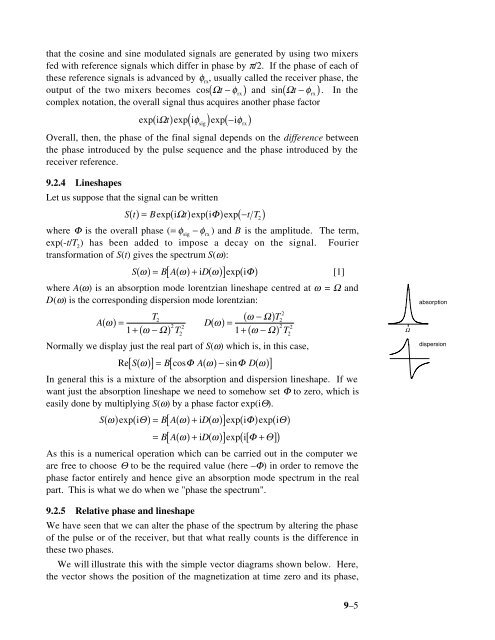
where A(ω) is an absorption mode lorentzian lineshape centred at ω = Ω and
D(ω) is the corresponding dispersion mode lorentzian:
2
T2
ω − Ω T2
A( ω)= D( ω)=
+ ( ω − )
2 2
2 2
1 Ω T2
1+ ( ω −Ω)
T2
Normally we display just the real part of S(ω) which is, in this case,
rx
( )
[ ( )]= ( )− ( )
[ ]
Re S ω B cosΦ
A ω sinΦ
D ω
In general this is a mixture of the absorption and dispersion lineshape. If we
want just the absorption lineshape we need to somehow set Φ to zero, which is
easily done by multiplying S(ω) by a phase factor exp(iΘ).
S( ω) exp( iΘ)= B[ A( ω)+ iD( ω)
] exp( iΦ) exp( iΘ)
= BA( ω)+ iD( ω)
exp i Φ Θ
[ ] ( [ + ])
As this is a numerical operation which can be carried out in the computer we
are free to choose Θ to be the required value (here –Φ) in order to remove the
phase factor entirely and hence give an absorption mode spectrum in the real
part. This is what we do when we "phase the spectrum".
9.2.5 Relative phase and lineshape
We have seen that we can alter the phase of the spectrum by altering the phase
of the pulse or of the receiver, but that what really counts is the difference in
these two phases.
We will illustrate this with the simple vector diagrams shown below. Here,
the vector shows the position of the magnetization at time zero and its phase,
Ω
absorption
dispersion
9–5