Phase Cycling and Gradient Pulses - The James Keeler Group

t 1 = 0
t 1 = ∆
t 1 = 2∆
t 1 = 3∆
x
t 1 = 4∆
–y
–x
y
x
t 2
t 2
t 2
t 2
t 1
t 2
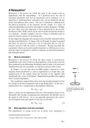
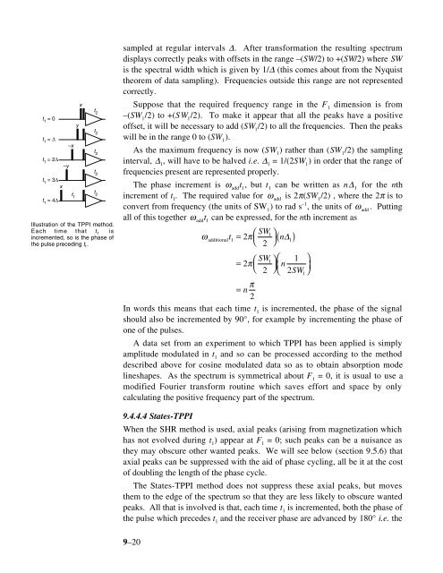
Illustration of the TPPI method.
Each time that t 1 is
incremented, so is the phase of
the pulse preceding t 1 .
sampled at regular intervals ∆. After transformation the resulting spectrum
displays correctly peaks with offsets in the range –(SW/2) to +(SW/2) where SW
is the spectral width which is given by 1/∆ (this comes about from the Nyquist
theorem of data sampling). Frequencies outside this range are not represented
correctly.
Suppose that the required frequency range in the F 1
dimension is from
–(SW 1
/2) to +(SW 1
/2). To make it appear that all the peaks have a positive
offset, it will be necessary to add (SW 1
/2) to all the frequencies. Then the peaks
will be in the range 0 to (SW 1
).
As the maximum frequency is now (SW 1
) rather than (SW 1
/2) the sampling
interval, ∆ 1
, will have to be halved i.e. ∆ 1
= 1/(2SW 1
) in order that the range of
frequencies present are represented properly.
The phase increment is ω add
t 1
, but t 1
can be written as n∆ 1
for the nth
increment of t 1
. The required value for ω add
is 2π(SW 1
/2) , where the 2π is to
convert from frequency (the units of SW 1
) to rad s –1 , the units of ω add
. Putting
all of this together ω add
t 1
can be expressed, for the nth increment as
ω t SW1
additional 1
= 2π
⎛ ⎞ n
1
⎝ 2 ⎠ ( ∆ )
SW1
1
= 2π
⎛ ⎞⎛
⎞ n
⎝ 2 ⎠⎜
⎟
⎝ 2 SW
1 ⎠
π
= n
2
In words this means that each time t 1
is incremented, the phase of the signal
should also be incremented by 90°, for example by incrementing the phase of
one of the pulses.
A data set from an experiment to which TPPI has been applied is simply
amplitude modulated in t 1
and so can be processed according to the method
described above for cosine modulated data so as to obtain absorption mode
lineshapes. As the spectrum is symmetrical about F 1
= 0, it is usual to use a
modified Fourier transform routine which saves effort and space by only
calculating the positive frequency part of the spectrum.
9.4.4.4 States-TPPI
When the SHR method is used, axial peaks (arising from magnetization which
has not evolved during t 1
) appear at F 1
= 0; such peaks can be a nuisance as
they may obscure other wanted peaks. We will see below (section 9.5.6) that
axial peaks can be suppressed with the aid of phase cycling, all be it at the cost
of doubling the length of the phase cycle.
The States-TPPI method does not suppress these axial peaks, but moves
them to the edge of the spectrum so that they are less likely to obscure wanted
peaks. All that is involved is that, each time t 1
is incremented, both the phase of
the pulse which precedes t 1
and the receiver phase are advanced by 180° i.e. the
9–20