Phase Cycling and Gradient Pulses - The James Keeler Group

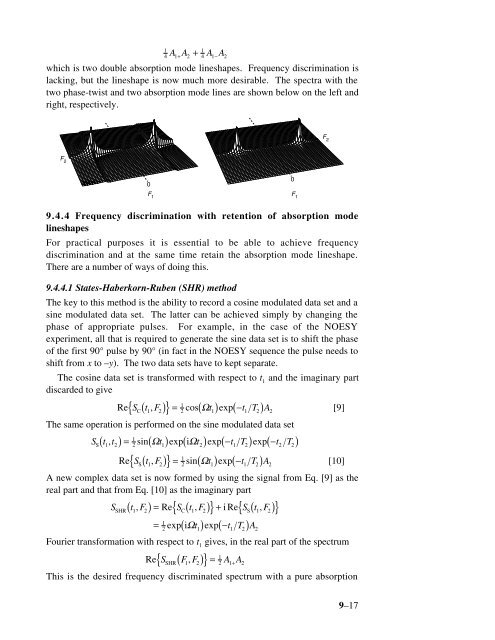
A A
+
A A
1
1
4 1+ 2 4 1−
2
which is two double absorption mode lineshapes. Frequency discrimination is
lacking, but the lineshape is now much more desirable. The spectra with the
two phase-twist and two absorption mode lines are shown below on the left and
right, respectively.
F 2
F 1 F 1
F 2
0
0
9.4.4 Frequency discrimination with retention of absorption mode
lineshapes
For practical purposes it is essential to be able to achieve frequency
discrimination and at the same time retain the absorption mode lineshape.
There are a number of ways of doing this.
9.4.4.1 States-Haberkorn-Ruben (SHR) method
The key to this method is the ability to record a cosine modulated data set and a
sine modulated data set. The latter can be achieved simply by changing the
phase of appropriate pulses. For example, in the case of the NOESY
experiment, all that is required to generate the sine data set is to shift the phase
of the first 90° pulse by 90° (in fact in the NOESY sequence the pulse needs to
shift from x to –y). The two data sets have to kept separate.
The cosine data set is transformed with respect to t 1
and the imaginary part
discarded to give
{ C( 1 2)
}=
2 ( 1) ( −
1 2)
2
1
Re S t , F cos Ω t exp t T A
[9]
The same operation is performed on the sine modulated data set
1
S t , t sin Ωt exp iΩt exp t T exp t T
S
( 1 2)= 2 ( 1) ( 2) ( −
1 2) ( −
2 2)
1
Re { SS( t1, F2)
}=
2
sin( t1) exp( −t1 T2)
A2
Ω [10]
A new complex data set is now formed by using the signal from Eq. [9] as the
real part and that from Eq. [10] as the imaginary part
( )= { ( )}+ ( )
( )
{ }
S t , F Re S t , F i Re S t , F
SHR 1 2 C 1 2 S 1 2
1
=
2
exp( iΩt1) exp −t1 T2 A2
Fourier transformation with respect to t 1
gives, in the real part of the spectrum
1
Re { SSHR( F1 , F2
)}= 2
A1+
A2
This is the desired frequency discriminated spectrum with a pure absorption
9–17