Phase Cycling and Gradient Pulses - The James Keeler Group
Phase Cycling and Gradient Pulses - The James Keeler Group
Phase Cycling and Gradient Pulses - The James Keeler Group

Create successful ePaper yourself
Turn your PDF publications into a flip-book with our unique Google optimized e-Paper software.
<strong>and</strong> then further transformation with respect to t 1<br />
gives<br />
1<br />
SP ( F1,<br />
F2)= 4<br />
A1+ + iD1+<br />
A2 iD2<br />
[ ][ + ]<br />
<strong>The</strong> real part of this spectrum is<br />
1<br />
Re { SP( F1,<br />
F2)<br />
}= A<br />
+<br />
A − D<br />
+<br />
D<br />
[ ]<br />
4 1 2 1 2<br />
<strong>The</strong> quantity in the square brackets on the right represents a phase-twist<br />
lineshape at F 1<br />
= +Ω, F 2<br />
= Ω<br />
Perspective view <strong>and</strong> contour plot of the phase-twist lineshape. Negative contours are shown dashed.<br />
This lineshape is an inextricable mixture of absorption <strong>and</strong> dispersion, <strong>and</strong> it is<br />
very undesirable for high-resolution NMR. So, although a phase modulated<br />
signal gives us frequency discrimination, which is desirable, it also results in a<br />
phase-twist lineshape, which is not.<br />
<strong>The</strong> time domain signal for the amplitude modulated data set can be written<br />
as<br />
1<br />
S t , t cos Ωt exp iΩt exp t T exp t T<br />
C<br />
( )= ( ) ( ) ( − ) ( − )<br />
1 2<br />
2 1 2 1 2 2 2<br />
Fourier transformation with respect to t 2<br />
gives<br />
which can be rewritten as<br />
1<br />
S t , F cos Ωt exp t T A iD<br />
C<br />
( 1 2)= 2 ( 1) ( −<br />
1 2) [ 2<br />
+<br />
2]<br />
[ ] −<br />
( )= ( )+ ( − )<br />
( )[ + ]<br />
1<br />
SC t1, F2<br />
exp iΩt exp iΩt exp t T A iD<br />
4 1 1 1 2 2 2<br />
Fourier transformation with respect to t 1<br />
gives, in the real part of the spectrum<br />
{ ( )}= [ ]+<br />
4 [ 1 2 1 2]<br />
1<br />
1<br />
Re SC F1, F2<br />
4<br />
A1+ A2 – D1+<br />
D2<br />
A<br />
−A – D<br />
–<br />
D<br />
This corresponds to two phase-twist lineshapes, one at F 1<br />
= +Ω, F 2<br />
= Ω <strong>and</strong> the<br />
other at F 1<br />
= –Ω, F 2<br />
= Ω; the lack of frequency discrimination is evident.<br />
Further, the undesirable phase-twist lineshape is again present.<br />
<strong>The</strong> lineshape can be restored to the absorption mode by discarding the<br />
imaginary part of the time domain signal after the transformation with respect<br />
to t 2<br />
, i.e. by taking the real part<br />
{ C( 1 2)<br />
}=<br />
2 ( 1) ( −<br />
1 2)<br />
2<br />
1<br />
Re S t , F cos Ωt exp t T A<br />
Subsequent transformation with respect to t 1<br />
gives, in the real part<br />
9–16