Phase Cycling and Gradient Pulses - The James Keeler Group

More documents

Recommendations

Info

Using this, the effect of the phase shifted pulse on the initial state σ ( p) can be written U σ φ ( p) – 1 Uφ ( ) ( ) ( ) − ( ) ( ) p – 1 = exp −iφFz U0exp iφFz σ exp iφFz U0 exp iφFz The central three terms can be simplified by application of Eq. [2] giving ( ) ( − ) = ( ) p – 1 exp iφF σ exp iφF U exp ipφ σ z ( ) ( p) z 0 ( ) ( ) ( ) ( ) p p Uφσ U – 1 φ = ( pφ) − φFz U σ U – 1 exp i exp i 0 0 exp iφFz The central three terms can, from Eq. [5], be replaced by σ ( p' ) to give ( ) ( ) φ z p p U σ U – 1 = exp( ipφ) exp −iφF σ ' exp iφF φ Finally, Eq. [5] is applied again to give ( ) ( ) ( ) – ( p' ) φ p 1 U σ U exp i pφ exp –ip' φ σ φ = ( ) ( ) Defining ∆p = (p' – p) as the change is coherence order, this simplifies to z [7] p – 1 p' U σ U exp – i∆ pφ σ [8] φ ( ) ( ) φ = ( ) Equation [8] says that if the phase of a pulse which is causing a change in coherence order of ∆p is shifted by φ the coherence will acquire a phase label (–∆p φ). It is this property which enables us to separate different changes in coherence order from one another by altering the phase of the pulse. In the discussion so far it has been assumed that U φ represents a single pulse. However, any sequence of pulses and delays can be represented by a single unitary transformation, so Eq. [8] applies equally well to the effect of phase shifting all of the pulses in such a sequence. We will see that this property is often of use in writing phase cycles. If a series of phase shifted pulses (or pulse sandwiches) are applied a phase (–∆p φ) is acquired from each. The total phase is found by adding up these individual contributions. In an NMR experiment this total phase affects the signal which is recorded at the end of the sequence, even though the phase shift may have been acquired earlier in the pulse sequence. These phase shifts are, so to speak, carried forward. 9.3.4 Coherence transfer pathways diagrams In designing a multiple-pulse NMR experiment the intention is to have specific orders of coherence present at various points in the sequence. One way of indicating this is to use a coherence transfer pathway (CTP) diagram along with the timing diagram for the pulse sequence. An example of shown below, which gives the pulse sequence and CTP for the DQF COSY experiment. 9–12
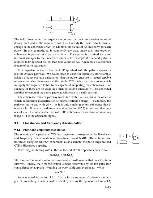
t 1 t 2 p 2 1 0 –1 –2 ∆p=±1 ±1,±3 +1,–3 The solid lines under the sequence represent the coherence orders required during each part of the sequence; note that it is only the pulses which cause a change in the coherence order. In addition, the values of ∆p are shown for each pulse. In this example, as is commonly the case, more than one order of coherence is present at a particular time. Each pulse is required to cause different changes to the coherence order – for example the second pulse is required to bring about no less than four values of ∆p. Again, this is a common feature of pulse sequences. It is important to realise that the CTP specified with the pulse sequence is just the desired pathway. We would need to establish separately (for example using a product operator calculation) that the pulse sequence is indeed capable of generating the coherences specified in the CTP. Also, the spin system which we apply the sequence to has to be capable of supporting the coherences. For example, if there are no couplings, then no double quantum will be generated and thus selection of the above pathway will result in a null spectrum. The coherence transfer pathway must start with p = 0 as this is the order to which equilibrium magnetization (z-magnetization) belongs. In addition, the pathway has to end with |p| = 1 as it is only single quantum coherence that is observable. If we use quadrature detection (section 9.2.2) it turns out that only one of p = ±1 is observable; we will follow the usual convention of assuming that p = –1 is the detectable signal. 9.4 Lineshapes and frequency discrimination 9.4.1 Phase and amplitude modulation –y The selection of a particular CTP has important consequences for lineshapes t 1 τ m t 2 and frequency discrimination in two-dimensional NMR. These topics are 1 illustrated using the NOESY experiment as an example; the pulse sequence and 0 –1 CTP is illustrated opposite. If we imagine starting with I z , then at the end of t 1 the operators present are − cosΩtI 1 y + sinΩtI 1 x The term in I y is rotated onto the z-axis and we will assume that only this term survives. Finally, the z-magnetization is made observable by the last pulse (for convenience set to phase –y) giving the observable term present at t 2 = 0 as cosΩt 1 I x As was noted in section 9.3.1, I x is in fact a mixture of coherence orders p = ±1, something which is made evident by writing the operator in terms of I + 9–13
Page 1 and 2: 9 Coherence Selection: Phase Cyclin
Page 3 and 4: We can go further with this interpr
Page 5 and 6: that the cosine and sine modulated
Page 7 and 8: y -x x -y pulse x y -x -y receiver
Page 9 and 10: phase cycling of many two- and thre
Page 11: ( ) ( )= ( ) exp −iΩtIz I± exp
Page 15 and 16: simply because cos(Ωt 1 ) = cos(-
Page 17 and 18: A A + A A 1 1 4 1+ 2 4 1− 2 which
Page 19 and 20: [ ] 1 S+ ( F1, F2)= 2 A1+ + iD1+ A2
Page 21 and 22: pulse goes x, -x and the receiver g
Page 23 and 24: step pulse phase phase shift experi
Page 25 and 26: As the cycle has four steps, a path
Page 27 and 28: dimensional spectra. This is consid
Page 29 and 30: doubles the length of the phase cyc
Page 31 and 32: t 1 τ mix t 2 1 0 -1 If we group t
Page 33 and 34: magnetic field is made spatially in
Page 35 and 36: 1.0 M x 0.5 0.0 10 20 30 40 50 γGr
Page 37 and 38: ∑ sp i iγ iBg,iτi = 0 . i With
Page 39 and 40: We start out the discussion by cons
Page 41 and 42: The sequence below shows the gradie
Page 43 and 44: stronger the gradient the more rapi
Page 45 and 46: discrimination in the F 1 dimension
Page 47 and 48: I ∆ 2 ∆ 2 ∆ 2 ∆ 2 t 2 S t 1
Page 49: y the gradient at the edges of the

Phase Cycling and Gradient Pulses - The James Keeler Group

Create successful ePaper yourself

Delete template?

Save as template?