Phase Cycling and Gradient Pulses - The James Keeler Group
Phase Cycling and Gradient Pulses - The James Keeler Group
Phase Cycling and Gradient Pulses - The James Keeler Group

Create successful ePaper yourself
Turn your PDF publications into a flip-book with our unique Google optimized e-Paper software.
9 Coherence Selection:<br />
<strong>Phase</strong> <strong>Cycling</strong> <strong>and</strong> <strong>Gradient</strong> <strong>Pulses</strong> †<br />
9.1 Introduction<br />
<strong>The</strong> pulse sequence used in an NMR experiment is carefully designed to<br />
produce a particular outcome. For example, we may wish to pass the spins<br />
through a state of multiple quantum coherence at a particular point, or plan for<br />
the magnetization to be aligned along the z-axis during a mixing period.<br />
However, it is usually the case that the particular series of events we designed<br />
the pulse sequence to cause is only one out of many possibilities. For example,<br />
a pulse whose role is to generate double-quantum coherence from anti-phase<br />
magnetization may also generate zero-quantum coherence or transfer the<br />
magnetization to another spin. Each time a radiofrequency pulse is applied<br />
there is this possibility of branching into many different pathways. If no steps<br />
are taken to suppress these unwanted pathways the resulting spectrum will be<br />
hopelessly confused <strong>and</strong> uninterpretable.<br />
<strong>The</strong>re are two general ways in which one pathway can be isolated from the<br />
many possible. <strong>The</strong> first is phase cycling. In this method the phases of the<br />
pulses <strong>and</strong> the receiver are varied in a systematic way so that the signal from<br />
the desired pathways adds <strong>and</strong> signal from all other pathways cancels. <strong>Phase</strong><br />
cycling requires that the experiment is repeated several times, something which<br />
is probably required in any case in order to achieve the required signal-to-noise<br />
ratio.<br />
<strong>The</strong> second method of selection is to use field gradient pulses. <strong>The</strong>se are<br />
short periods during which the applied magnetic field is made inhomogeneous.<br />
As a result, any coherences present dephase <strong>and</strong> are apparently lost. However,<br />
this dephasing can be undone, <strong>and</strong> the coherence restored, by application of a<br />
subsequent gradient. We shall see that this dephasing <strong>and</strong> rephasing approach<br />
can be used to select particular coherences. Unlike phase cycling, the use of<br />
field gradient pulses does not require repetition of the experiment.<br />
Both of these selection methods can be described in a unified framework<br />
which classifies the coherences present at any particular point according to a<br />
coherence order <strong>and</strong> then uses coherence transfer pathways to specify the<br />
desired outcome of the experiment.<br />
9.2 <strong>Phase</strong> in NMR<br />
In NMR we have control over both the phase of the pulses <strong>and</strong> the receiver<br />
phase. <strong>The</strong> effect of changing the phase of a pulse is easy to visualise in the<br />
usual rotating frame. So, for example, a 90° pulse about the x-axis rotates<br />
†<br />
Chapter 9 "Coherence Selection: <strong>Phase</strong> <strong>Cycling</strong> <strong>and</strong> <strong>Gradient</strong> <strong>Pulses</strong>" © <strong>James</strong> <strong>Keeler</strong> 2001<br />
<strong>and</strong> 2003.<br />
9–1
magnetization from z onto –y, whereas the same pulse applied about the y-axis<br />
rotates the magnetization onto the x-axis. <strong>The</strong> idea of the receiver phase is<br />
slightly more complex <strong>and</strong> will be explored in this section.<br />
<strong>The</strong> NMR signal – that is the free induction decay – which emerges from the<br />
probe is a radiofrequency signal oscillating at close to the Larmor frequency<br />
(usually hundreds of MHz). Within the spectrometer this signal is shifted down<br />
to a much lower frequency in order that it can be digitized <strong>and</strong> then stored in<br />
computer memory. <strong>The</strong> details of this down-shifting process can be quite<br />
complex, but the overall result is simply that a fixed frequency, called the<br />
receiver reference or carrier, is subtracted from the frequency of the incoming<br />
NMR signal. Frequently, this receiver reference frequency is the same as the<br />
transmitter frequency used to generate the pulses applied to the observed<br />
nucleus. We shall assume that this is the case from now on.<br />
<strong>The</strong> rotating frame which we use to visualise the effect of pulses is set at the<br />
transmitter frequency, ω rf<br />
, so that the field due to the radiofrequency pulse is<br />
static. In this frame, a spin whose Larmor frequency is ω 0<br />
precesses at (ω 0<br />
–<br />
ω rf<br />
), called the offset Ω. In the spectrometer the incoming signal at ω 0<br />
is downshifted<br />
by subtracting the receiver reference which, as we have already decided,<br />
will be equal to the frequency of the radiofrequency pulses. So, in effect, the<br />
frequencies of the signals which are digitized in the spectrometer are the offset<br />
frequencies at which the spins evolve in the rotating frame. Often this whole<br />
process is summarised by saying that the "signal is detected in the rotating<br />
frame".<br />
9.2.1 Detector phase<br />
<strong>The</strong> quantity which is actually detected in an NMR experiment is the transverse<br />
magnetization. Ultimately, this appears at the probe as an oscillating voltage,<br />
which we will write as<br />
S = cosω FID 0t<br />
where ω 0<br />
is the Larmor frequency. <strong>The</strong> down-shifting process in the<br />
spectrometer is achieved by an electronic device called a mixer; this effectively<br />
multiplies the incoming signal by a locally generated reference signal, S ref<br />
,<br />
which we will assume is oscillating at ω rf<br />
Sref<br />
= cosω<br />
rft<br />
<strong>The</strong> output of the mixer is the product S FID<br />
S ref<br />
S S = Acosω<br />
tcosω<br />
t<br />
9–2<br />
FID ref rf 0<br />
1<br />
=<br />
2<br />
A[ cos( ωrf<br />
+ ω0) t + cos( ωrf<br />
−ω0)<br />
t]<br />
<strong>The</strong> first term is an oscillation at a high frequency (of the order of twice the<br />
Larmor frequency as ω 0<br />
≈ ω rf<br />
) <strong>and</strong> is easily removed by a low-pass filter. <strong>The</strong><br />
second term is an oscillation at the offset frequency, Ω. This is in line with the<br />
previous comment that this down-shifting process is equivalent to detecting the<br />
precession in the rotating frame.
We can go further with this interpretation <strong>and</strong> say that the second term<br />
represents the component of the magnetization along a particular axis (called<br />
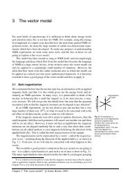
the reference axis) in the rotating frame. Such a component varies as cos Ωt,<br />
assuming that at time zero the magnetization is aligned along the chosen axis;<br />
this is illustrated below<br />
θ<br />
t = 0<br />
time t<br />
At time zero the magnetization is assumed to be aligned along the reference axis. After time t the<br />
magnetization has precessed through an angle θ = Ωt. <strong>The</strong> projection of the magnetization onto the<br />
reference axis is proportional to cos Ωt.<br />
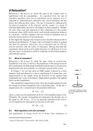
Suppose now that the phase of the reference signal is shifted by φ, something<br />
which is easily achieved in the spectrometer. Effectively, this shifts the<br />
reference axis by φ, as shown below<br />
φ<br />
θ–<br />
φ<br />
t = 0<br />
time t<br />
Shifting the phase of the receiver reference by φ is equivalent to detecting the component along an axis<br />
rotated by φ from its original position (the previous axis is shown in grey). Now the apparent angle of<br />
precession is θ = Ωt – φ. <strong>and</strong> the projection of the magnetization onto the reference axis is proportional to<br />
cos (Ωt – φ).<br />
( )<br />
<strong>The</strong> component along the new reference axis is proportional to cos Ωt − φ .<br />
How this is put to good effect is described in the next section.<br />
9–3
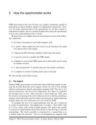
y<br />
<strong>The</strong> x <strong>and</strong> y projections of the<br />
black vector are both positive.<br />
If the vector had precessed in<br />
the opposite direction (shown<br />
shaded), <strong>and</strong> at the same<br />
frequency, the projection along<br />
x would be the same, but along<br />
y it would be minus that of the<br />
black vector.<br />
θ<br />
x<br />
9.2.2 Quadrature detection<br />
We normally want to place the transmitter frequency in the centre of the<br />
resonances of interest so as to minimise off-resonance effects. If the receiver<br />
reference frequency is the same as the transmitter frequency, it immediately<br />
follows that the offset frequencies, Ω, may be both positive <strong>and</strong> negative.<br />
However, as we have seen in the previous section the effect of the downshifting<br />
scheme used is to generate a signal of the form cos Ωt. Since cos(θ) =<br />
cos(–θ) such a signal does not discriminate between positive <strong>and</strong> negative<br />
offset frequencies. <strong>The</strong> resulting spectrum, obtained by Fourier transformation,<br />
would be confusing as each peak would appear at both +Ω <strong>and</strong> –Ω.<br />
<strong>The</strong> way out of this problem is to detect the signal along two perpendicular<br />
axes. As is illustrated opposite, the projection along one axis is proportional to<br />
cos(Ωt) <strong>and</strong> to sin(Ωt) along the other. Knowledge of both of these projections<br />
enables us to work out the sense of rotation of the vector i.e. the sign of the<br />
offset.<br />
<strong>The</strong> sin modulated component is detected by having a second mixer fed with<br />
a reference whose phase is shifted by π/2. Following the above discussion the<br />
output of the mixer is<br />
cos( Ωt−<br />
π 2)= cosΩtcosπ 2+<br />
sinΩtsinπ<br />
2<br />
= sinΩt<br />
<strong>The</strong> output of these two mixers can be regarded as being the components of the<br />
magnetization along perpendicular axes in the rotating frame.<br />
<strong>The</strong> final step in this whole process is regard the outputs of the two mixers as<br />
being the real <strong>and</strong> imaginary parts of a complex number:<br />
cosΩt + isinΩt = exp( iΩt)<br />
<strong>The</strong> overall result is the generation of a complex signal whose phase varies<br />
according to the offset frequency Ω.<br />
9.2.3 Control of phase<br />
In the previous section we supposed that the signal coming from the probe was<br />
of the form cosω 0<br />
t but it is more realistic to write the signal as<br />
cos(ω 0<br />
t + φ sig<br />
) in recognition of the fact that in addition to a frequency the signal<br />
has a phase, φ sig<br />
. This phase is a combination of factors that are not under our<br />
control (such as phase shifts produced in the amplifiers <strong>and</strong> filters through<br />
which the signal passes) <strong>and</strong> a phase due to the pulse sequence, which certainly<br />
is under our control.<br />
<strong>The</strong> overall result of this phase is simply to multiply the final complex signal<br />
by a phase factor, exp(iφ sig<br />
):<br />
( ) ( iφ<br />
sig )<br />
exp iΩt<br />
exp<br />
As we saw in the previous section, we can also introduce another phase shift by<br />
altering the phase of the reference signal fed to the mixer, <strong>and</strong> indeed we saw<br />
9–4
that the cosine <strong>and</strong> sine modulated signals are generated by using two mixers<br />
fed with reference signals which differ in phase by π/2. If the phase of each of<br />
these reference signals is advanced by φ rx<br />
, usually called the receiver phase, the<br />
output of the two mixers becomes cos( Ωt − φ rx ) <strong>and</strong> sin( Ωt − φ rx ). In the<br />
complex notation, the overall signal thus acquires another phase factor<br />
( ) ( ) −<br />
exp iΩt<br />
exp iφ<br />
exp iφ<br />
sig<br />
( )<br />
Overall, then, the phase of the final signal depends on the difference between<br />
the phase introduced by the pulse sequence <strong>and</strong> the phase introduced by the<br />
receiver reference.<br />
9.2.4 Lineshapes<br />
Let us suppose that the signal can be written<br />
St ()= Bexp( iΩt) exp( iΦ) exp( −tT2<br />
)<br />
where Φ is the overall phase (= φsig<br />
−φrx ) <strong>and</strong> B is the amplitude. <strong>The</strong> term,<br />
exp(-t/T 2<br />
) has been added to impose a decay on the signal. Fourier<br />
transformation of S(t) gives the spectrum S(ω):<br />
S( ω)= B[ A( ω)+ iD( ω)<br />
] exp( iΦ )<br />
[1]<br />
where A(ω) is an absorption mode lorentzian lineshape centred at ω = Ω <strong>and</strong><br />
D(ω) is the corresponding dispersion mode lorentzian:<br />
2<br />
T2<br />
ω − Ω T2<br />
A( ω)= D( ω)=<br />
+ ( ω − )<br />
2 2<br />
2 2<br />
1 Ω T2<br />
1+ ( ω −Ω)<br />
T2<br />
Normally we display just the real part of S(ω) which is, in this case,<br />
rx<br />
( )<br />
[ ( )]= ( )− ( )<br />
[ ]<br />
Re S ω B cosΦ<br />
A ω sinΦ<br />
D ω<br />
In general this is a mixture of the absorption <strong>and</strong> dispersion lineshape. If we<br />
want just the absorption lineshape we need to somehow set Φ to zero, which is<br />
easily done by multiplying S(ω) by a phase factor exp(iΘ).<br />
S( ω) exp( iΘ)= B[ A( ω)+ iD( ω)<br />
] exp( iΦ) exp( iΘ)<br />
= BA( ω)+ iD( ω)<br />
exp i Φ Θ<br />
[ ] ( [ + ])<br />
As this is a numerical operation which can be carried out in the computer we<br />
are free to choose Θ to be the required value (here –Φ) in order to remove the<br />
phase factor entirely <strong>and</strong> hence give an absorption mode spectrum in the real<br />
part. This is what we do when we "phase the spectrum".<br />
9.2.5 Relative phase <strong>and</strong> lineshape<br />
We have seen that we can alter the phase of the spectrum by altering the phase<br />
of the pulse or of the receiver, but that what really counts is the difference in<br />
these two phases.<br />
We will illustrate this with the simple vector diagrams shown below. Here,<br />
the vector shows the position of the magnetization at time zero <strong>and</strong> its phase,<br />
Ω<br />
absorption<br />
dispersion<br />
9–5
φ sig<br />
, is measured anti-clockwise from the x-axis. <strong>The</strong> dot shows the axis along<br />
which the receiver is aligned; this phase, φ rx<br />
, is also measured anti-clockwise<br />
from the x-axis.<br />
If the vector <strong>and</strong> receiver are aligned along the same axis, Φ = 0, <strong>and</strong> the real<br />
part of the spectrum shows the absorption mode lineshape. If the receiver<br />
phase is advanced by π/2, Φ = 0 – π/2 <strong>and</strong>, from Eq. [1]<br />
S( ω)= B[ A( ω)+ iD( ω)<br />
] exp( −iπ<br />
2)<br />
= B − iA( ω)+ D( ω)<br />
[ ]<br />
This means that the real part of the spectrum shows a dispersion lineshape. On<br />
the other h<strong>and</strong>, if the magnetization is advanced by π/2, Φ = φ sig<br />
– φ rx<br />
= π/2 – 0 = π/2 <strong>and</strong> it can be shown from Eq. [1] that the real part of the<br />
spectrum shows a negative dispersion lineshape. Finally, if either phase is<br />
advanced by π, the result is a negative absorption lineshape.<br />
y<br />
x<br />
φ rx<br />
φ<br />
9.2.6 CYCLOPS<br />
<strong>The</strong> CYCLOPS phase cycling scheme is commonly used in even the simplest<br />
pulse-acquire experiments. <strong>The</strong> sequence is designed to cancel some<br />
imperfections associated with errors in the two phase detectors mentioned<br />
above; a description of how this is achieved is beyond the scope of this<br />
discussion. However, the cycle itself illustrates very well the points made in<br />
the previous section.<br />
<strong>The</strong>re are four steps in the cycle, the pulse phase goes x, y, –x, –y i.e. it<br />
advances by 90° on each step; likewise the receiver advances by 90° on each<br />
step. <strong>The</strong> figure below shows how the magnetization <strong>and</strong> receiver phases are<br />
related for the four steps of this cycle<br />
9–6
y<br />
–x<br />
x<br />
–y<br />
pulse x y –x –y<br />
receiver x y –x –y<br />
Although both the receiver <strong>and</strong> the magnetization shift phase on each step, the<br />
phase difference between them remains constant. Each step in the cycle thus<br />
gives the same lineshape <strong>and</strong> so the signal adds on all four steps, which is just<br />
what is required.<br />
Suppose that we forget to advance the pulse phase; the outcome is quite<br />
different<br />
pulse x x x x<br />
receiver x y –x –y<br />
y<br />
–x<br />
x<br />
–y<br />
Now the phase difference between the receiver <strong>and</strong> the magnetization is no<br />
longer constant. A different lineshape thus results from each step <strong>and</strong> it is clear<br />
that adding all four together will lead to complete cancellation (steps 2 <strong>and</strong> 4<br />
cancel, as do steps 1 <strong>and</strong> 3). For the signal to add up it is clearly essential for<br />
the receiver to follow the magnetization.<br />
9.2.7 EXORCYLE<br />
EXORCYLE is perhaps the original phase cycle. It is a cycle used for 180°<br />
pulses when they form part of a spin echo sequence. <strong>The</strong> 180° pulse cycles<br />
through the phases x, y, –x, –y <strong>and</strong> the receiver phase goes x, –x, x, –x. <strong>The</strong><br />
diagram below illustrates the outcome of this sequence<br />
9–7
y<br />
y<br />
180°(±x)<br />
τ<br />
90°(x) – τ<br />
–x<br />
x<br />
–y<br />
180°(±y)<br />
τ<br />
If the phase of the 180° pulse is +x or –x the echo forms along the y-axis,<br />
whereas if the phase is ±y the echo forms on the –y axis. <strong>The</strong>refore, as the 180°<br />
pulse is advanced by 90° (e.g. from x to y) the receiver must be advanced by<br />
180° (e.g. from x to –x). Of course, we could just as well cycle the receiver<br />
phases y, –y, y, –y; all that matters is that they advance in steps of 180°. We<br />
will see later on how it is that this phase cycle cancels out the results of<br />
imperfections in the 180° pulse.<br />
–y<br />
I<br />
S<br />
1<br />
2J<br />
y<br />
1<br />
2J<br />
Pulse sequence for INEPT.<br />
Filled rectangles represent 90°<br />
pulses <strong>and</strong> open rectangles<br />
represent 180° pulses. Unless<br />
otherwise indicated, all pulses<br />
are of phase x.<br />
9.2.8 Difference spectroscopy<br />
Often a simple two step sequence suffices to cancel unwanted magnetization;<br />
essentially this is a form of difference spectroscopy. <strong>The</strong> idea is well illustrated<br />
by the INEPT sequence, shown opposite. <strong>The</strong> aim of the sequence is to transfer<br />
magnetization from spin I to a coupled spin S.<br />
With the phases <strong>and</strong> delays shown equilibrium magnetization of spin I, I z<br />
, is<br />
transferred to spin S, appearing as the operator S x<br />
. Equilibrium magnetization<br />
of S, S z<br />
, appears as S y<br />
. We wish to preserve only the signal that has been<br />
transferred from I.<br />
<strong>The</strong> procedure to achieve this is very simple. If we change the phase of the<br />
second I spin 90° pulse from y to –y the magnetization arising from transfer of<br />
the I spin magnetization to S becomes –S x<br />
i.e. it changes sign. In contrast, the<br />
signal arising from equilibrium S spin magnetization is unaffected simply<br />
because the S z<br />
operator is unaffected by the I spin pulses. By repeating the<br />
experiment twice, once with the phase of the second I spin 90° pulse set to y<br />
<strong>and</strong> once with it set to –y, <strong>and</strong> then subtracting the two resulting signals, the<br />
undesired signal is cancelled <strong>and</strong> the desired signal adds. It is easily confirmed<br />
that shifting the phase of the S spin 90° pulse does not achieve the desired<br />
separation of the two signals as both are affected in the same way.<br />
In practice the subtraction would be carried out by shifting the receiver by<br />
180°, so the I spin pulse would go y, –y <strong>and</strong> the receiver phase go x, –x. This is<br />
a two step phase cycle which is probably best viewed as difference<br />
spectroscopy.<br />
This simple two step cycle is the basic element used in constructing the<br />
9–8
phase cycling of many two- <strong>and</strong> three-dimensional heteronuclear experiments.<br />
9.3 Coherence transfer pathways<br />
Although we can make some progress in writing simple phase cycles by<br />
considering the vector picture, a more general framework is needed in order to<br />
cope with experiments which involve multiple-quantum coherence <strong>and</strong> related<br />
phenomena. We also need a theory which enables us to predict the degree to<br />
which a phase cycle can discriminate against different classes of unwanted<br />
signals. A convenient <strong>and</strong> powerful way of doing both these things is to use the<br />
coherence transfer pathway approach.<br />
9.3.1 Coherence order<br />
Coherences, of which transverse magnetization is one example, can be<br />
classified according to a coherence order, p, which is an integer taking values 0,<br />
± 1, ± 2 ... Single quantum coherence has p = ± 1, double has<br />
p = ± 2 <strong>and</strong> so on; z-magnetization, "zz" terms <strong>and</strong> zero-quantum coherence<br />
have p = 0. This classification comes about by considering the phase which<br />
different coherences acquire is response to a rotation about the z-axis.<br />
A coherence of order p, represented by the density operator σ ( p)<br />
, evolves<br />
under a z-rotation of angle φ according to<br />
( ) ( )= ( − )<br />
( ) ( )<br />
p<br />
p<br />
exp −iφFz<br />
σ exp iφFz<br />
exp ipφ σ<br />
[2]<br />
where F z<br />
is the operator for the total z-component of the spin angular<br />
momentum. In words, a coherence of order p experiences a phase shift of –pφ.<br />
Equation [2] is the definition of coherence order.<br />
To see how this definition can be applied, consider the effect of a z-rotation<br />
on transverse magnetization aligned along the x-axis. Such a rotation is<br />
identical in nature to that due to evolution under an offset, <strong>and</strong> using product<br />
operators it can be written<br />
( ) ( )= +<br />
exp −iφI I exp iφI cosφ I sinφ<br />
I<br />
z x z x y [3]<br />
<strong>The</strong> right h<strong>and</strong> sides of Eqs. [2] <strong>and</strong> [3] are not immediately comparable, but by<br />
writing the sine <strong>and</strong> cosine terms as complex exponentials the comparison<br />
becomes clearer. Using<br />
[ ( )] =<br />
2i<br />
( )− ( − )<br />
[ ]<br />
1<br />
1<br />
cosφ = exp( iφ)+ exp −i φ sinφ exp iφ exp iφ<br />
Eq. [3] becomes<br />
2<br />
( z) x ( z)<br />
( )<br />
exp −iφI I exp iφI<br />
[ ] + [ ( )− ( − )]<br />
1<br />
1<br />
=<br />
2<br />
exp( iφ)+ exp −iφ Ix<br />
2i<br />
exp iφ exp iφ<br />
I<br />
1 1 1 1<br />
=<br />
2 [ Ix +<br />
i<br />
Iy] exp( iφ)+ 2 [ Ix −<br />
i<br />
Iy] exp( −iφ)<br />
It is now clear that the first term corresponds to coherence order –1 <strong>and</strong> the<br />
second to +1; in other words, I x<br />
is an equal mixture of coherence orders ±1.<br />
<strong>The</strong> cartesian product operators do not correspond to a single coherence<br />
y<br />
9–9
order so it is more convenient to rewrite them in terms of the raising <strong>and</strong><br />
lowering operators, I +<br />
<strong>and</strong> I –<br />
, defined as<br />
I = I + i x<br />
Iy I =<br />
+<br />
I i<br />
– x<br />
– Iy<br />
from which it follows that<br />
I = 1<br />
I +<br />
1<br />
x 2 [ +<br />
I– ] Iy =<br />
2i [ I+<br />
− I–<br />
]<br />
[4]<br />
Under z-rotations the raising <strong>and</strong> lowering operators transform simply<br />
( ) ( )= ( )<br />
exp −iφIz I± exp iφIz exp miφ<br />
I±<br />
which, by comparison with Eq. [2] shows that I +<br />
corresponds to coherence<br />
order +1 <strong>and</strong> I –<br />
to –1. So, from Eq. [4] we can see that I x<br />
<strong>and</strong> I y<br />
correspond to<br />
mixtures of coherence orders +1 <strong>and</strong> –1.<br />
As a second example consider the pure double quantum operator for two<br />
coupled spins,<br />
2I I + 2I I<br />
1x 2y 1y 2x<br />
Rewriting this in terms of the raising <strong>and</strong> lowering operators gives<br />
1 + + − −<br />
i ( I1 I2 − I1 I2)<br />
+ +<br />
<strong>The</strong> effect of a z-rotation on the term I1 I is found as follows:<br />
2<br />
exp −iφI exp iφI I I exp iφI exp iφI<br />
( 1z) ( −<br />
2z) 1+ 2+<br />
( 2z) ( 1z)<br />
( 1z) ( − ) 1+ 2+<br />
( 1z)<br />
( ) ( − ) = ( − )<br />
= exp −iφI exp iφ I I exp iφI<br />
= exp −iφ exp iφ I1+ I2+ exp 2iφ<br />
I1+ I2+<br />
Thus, as the coherence experiences a phase shift of –2φ the coherence is<br />
classified according to Eq. [2] as having p = 2. It is easy to confirm that the<br />
term I1 I has p = –2. Thus the pure double quantum term,<br />
− 2− 2I1xI2y + 2I1yI<br />
, is<br />
2x<br />
an equal mixture of coherence orders +2 <strong>and</strong> –2.<br />
As this example indicates, it is possible to determine the order or orders of<br />
any state by writing it in terms of raising <strong>and</strong> lowering operators <strong>and</strong> then<br />
simply inspecting the number of such operators in each term. A raising<br />
operator contributes +1 to the coherence order whereas a lowering operator<br />
contributes –1. A z-operator, I iz , has coherence order 0 as it is invariant to z-<br />
rotations.<br />
Coherences involving heteronuclei can be assigned both an overall order <strong>and</strong><br />
an order with respect to each nuclear species. For example the term I1 S has<br />
+ 1– an overall order of 0, is order +1 for the I spins <strong>and</strong> –1 for the S spins. <strong>The</strong> term<br />
I 1+ I 2+ S 1z<br />
is overall of order 2, is order 2 for the I spins <strong>and</strong> is order 0 for the S<br />
spins.<br />
9.3.2 Evolution under offsets<br />
<strong>The</strong> evolution under an offset, Ω, is simply a z-rotation, so the raising <strong>and</strong><br />
lowering operators simply acquire a phase Ωt<br />
9–10
( ) ( )= ( )<br />
exp −iΩtIz I± exp iΩtIz exp miΩt I±<br />
For products of these operators, the overall phase is the sum of the phases<br />
acquired by each term<br />
( j jz ) ( −<br />
i iz ) i− j + ( i iz ) ( j jz )<br />
( i j)<br />
tIi− Ij+<br />
exp −iΩ tI exp iΩtI I I exp iΩtI exp iΩ<br />
tI<br />
( )<br />
= exp i Ω −Ω<br />
It also follows that coherences of opposite sign acquire phases of opposite signs<br />
under free evolution. So the operator I 1+<br />
I 2+<br />
(with p = 2) acquires a phase –(Ω 1<br />
+<br />
Ω 2<br />
)t i.e. it evolves at a frequency –(Ω 1<br />
+ Ω 2<br />
) whereas the operator I 1–<br />
I 2–<br />
(with p<br />
= –2) acquires a phase (Ω 1<br />
+ Ω 2<br />
)t i.e. it evolves at a frequency (Ω 1<br />
+ Ω 2<br />
). We<br />
will see later on that this observation has important consequences for the<br />
lineshapes in two-dimensional NMR.<br />
<strong>The</strong> observation that coherences of different orders respond differently to<br />
evolution under a z-rotation (e.g. an offset) lies at the heart of the way in which<br />
gradient pulses can be used to separate different coherence orders.<br />
9.3.3 <strong>Phase</strong> shifted pulses<br />
In general, a radiofrequency pulse causes coherences to be transferred from one<br />
order to one or more different orders; it is this spreading out of the coherence<br />
which makes it necessary to select one transfer among many possibilities. An<br />
example of this spreading between coherence orders is the effect of a nonselective<br />
pulse on antiphase magnetization, such as 2I 1x<br />
I 2z<br />
, which corresponds to<br />
coherence orders ±1. Some of the coherence may be transferred into double<strong>and</strong><br />
zero-quantum coherence, some may be transferred into two-spin order <strong>and</strong><br />
some will remain unaffected. <strong>The</strong> precise outcome depends on the phase <strong>and</strong><br />
flip angle of the pulse, but in general we can see that there are many<br />
possibilities.<br />
If we consider just one coherence, of order p, being transferred to a<br />
coherence of order p' by a radiofrequency pulse we can derive a very general<br />
result for the way in which the phase of the pulse affects the phase of the<br />
coherence. It is on this relationship that the phase cycling method is based.<br />
We will write the initial state of order p as σ ( p)<br />
, <strong>and</strong> the final state of order p'<br />
as σ ( p' ) . <strong>The</strong> effect of the radiofrequency pulse causing the transfer is<br />
represented by the (unitary) transformation U φ<br />
where φ is the phase of the<br />
pulse. <strong>The</strong> initial <strong>and</strong> final states are related by the usual transformation<br />
( ) ( )<br />
U<br />
p – 1<br />
U<br />
p '<br />
0σ<br />
0<br />
= σ + terms of other orders [5]<br />
which has been written for phase 0; the other terms will be dropped as we are<br />
only interested in the transfer from p to p'. <strong>The</strong> transformation brought about<br />
by a radiofrequency pulse phase shifted by φ, U φ<br />
, is related to that with the<br />
phase set to zero, U 0<br />
, in the following way<br />
( ) ( )<br />
Uφ = exp −iφFz<br />
U0 exp iφFz<br />
[6]<br />
9–11
Using this, the effect of the phase shifted pulse on the initial state σ ( p)<br />
can be<br />
written<br />
U σ<br />
φ<br />
( p)<br />
– 1<br />
Uφ<br />
( ) ( )<br />
( )<br />
−<br />
( ) ( )<br />
p<br />
– 1<br />
= exp −iφFz<br />
U0exp iφFz<br />
σ exp iφFz<br />
U0<br />
exp iφFz<br />
<strong>The</strong> central three terms can be simplified by application of Eq. [2]<br />
giving<br />
( ) ( − ) = ( )<br />
p<br />
– 1<br />
exp iφF σ exp iφF U exp ipφ σ<br />
z<br />
( ) ( p)<br />
z 0<br />
( ) ( )<br />
( ) ( )<br />
p<br />
p<br />
Uφσ U – 1<br />
φ<br />
= ( pφ) − φFz<br />
U σ U – 1<br />
exp i exp i<br />
0 0<br />
exp iφFz<br />
<strong>The</strong> central three terms can, from Eq. [5], be replaced by σ ( p' ) to give<br />
( ) ( )<br />
φ<br />
z<br />
p<br />
p<br />
U σ U – 1<br />
= exp( ipφ) exp −iφF σ '<br />
exp iφF<br />
φ<br />
Finally, Eq. [5] is applied again to give<br />
( ) ( )<br />
( ) – ( p'<br />
)<br />
φ<br />
p 1<br />
U σ U exp i pφ exp –ip'<br />
φ σ<br />
φ<br />
= ( ) ( )<br />
Defining ∆p = (p' – p) as the change is coherence order, this simplifies to<br />
z<br />
[7]<br />
p – 1<br />
p'<br />
U σ U exp – i∆ pφ σ<br />
[8]<br />
φ<br />
( ) ( )<br />
φ<br />
= ( )<br />
Equation [8] says that if the phase of a pulse which is causing a change in<br />
coherence order of ∆p is shifted by φ the coherence will acquire a phase label<br />
(–∆p φ). It is this property which enables us to separate different changes in<br />
coherence order from one another by altering the phase of the pulse.<br />
In the discussion so far it has been assumed that U φ<br />
represents a single pulse.<br />
However, any sequence of pulses <strong>and</strong> delays can be represented by a single<br />
unitary transformation, so Eq. [8] applies equally well to the effect of phase<br />
shifting all of the pulses in such a sequence. We will see that this property is<br />
often of use in writing phase cycles.<br />
If a series of phase shifted pulses (or pulse s<strong>and</strong>wiches) are applied a phase<br />
(–∆p φ) is acquired from each. <strong>The</strong> total phase is found by adding up these<br />
individual contributions. In an NMR experiment this total phase affects the<br />
signal which is recorded at the end of the sequence, even though the phase shift<br />
may have been acquired earlier in the pulse sequence. <strong>The</strong>se phase shifts are,<br />
so to speak, carried forward.<br />
9.3.4 Coherence transfer pathways diagrams<br />
In designing a multiple-pulse NMR experiment the intention is to have specific<br />
orders of coherence present at various points in the sequence. One way of<br />
indicating this is to use a coherence transfer pathway (CTP) diagram along<br />
with the timing diagram for the pulse sequence. An example of shown below,<br />
which gives the pulse sequence <strong>and</strong> CTP for the DQF COSY experiment.<br />
9–12
t 1 t 2<br />
p<br />
2<br />
1<br />
0<br />
–1<br />
–2<br />
∆p=±1 ±1,±3<br />
+1,–3<br />
<strong>The</strong> solid lines under the sequence represent the coherence orders required<br />
during each part of the sequence; note that it is only the pulses which cause a<br />
change in the coherence order. In addition, the values of ∆p are shown for each<br />
pulse. In this example, as is commonly the case, more than one order of<br />
coherence is present at a particular time. Each pulse is required to cause<br />
different changes to the coherence order – for example the second pulse is<br />
required to bring about no less than four values of ∆p. Again, this is a common<br />
feature of pulse sequences.<br />
It is important to realise that the CTP specified with the pulse sequence is<br />
just the desired pathway. We would need to establish separately (for example<br />
using a product operator calculation) that the pulse sequence is indeed capable<br />
of generating the coherences specified in the CTP. Also, the spin system which<br />
we apply the sequence to has to be capable of supporting the coherences. For<br />
example, if there are no couplings, then no double quantum will be generated<br />
<strong>and</strong> thus selection of the above pathway will result in a null spectrum.<br />
<strong>The</strong> coherence transfer pathway must start with p = 0 as this is the order to<br />
which equilibrium magnetization (z-magnetization) belongs. In addition, the<br />
pathway has to end with |p| = 1 as it is only single quantum coherence that is<br />
observable. If we use quadrature detection (section 9.2.2) it turns out that only<br />
one of p = ±1 is observable; we will follow the usual convention of assuming<br />
that p = –1 is the detectable signal.<br />
9.4 Lineshapes <strong>and</strong> frequency discrimination<br />
9.4.1 <strong>Phase</strong> <strong>and</strong> amplitude modulation<br />
–y<br />
<strong>The</strong> selection of a particular CTP has important consequences for lineshapes<br />
t 1 τ m<br />
t 2<br />
<strong>and</strong> frequency discrimination in two-dimensional NMR. <strong>The</strong>se topics are<br />
1<br />
illustrated using the NOESY experiment as an example; the pulse sequence <strong>and</strong> 0<br />
–1<br />
CTP is illustrated opposite.<br />
If we imagine starting with I z<br />
, then at the end of t 1<br />
the operators present are<br />
− cosΩtI<br />
1 y<br />
+ sinΩtI<br />
1 x<br />
<strong>The</strong> term in I y<br />
is rotated onto the z-axis <strong>and</strong> we will assume that only this term<br />
survives. Finally, the z-magnetization is made observable by the last pulse (for<br />
convenience set to phase –y) giving the observable term present at t 2<br />
= 0 as<br />
cosΩt 1<br />
I x<br />
As was noted in section 9.3.1, I x<br />
is in fact a mixture of coherence orders<br />
p = ±1, something which is made evident by writing the operator in terms of I +<br />
9–13
1<br />
0<br />
–1<br />
–y<br />
t 1 τ m<br />
t 2<br />
<strong>and</strong> I –<br />
1<br />
cosΩt ( I + I )<br />
9–14<br />
2 1<br />
+ −<br />
Of these operators, only I –<br />
leads to an observable signal, as this corresponds to<br />
p = –1. Allowing I –<br />
to evolve in t 2<br />
gives<br />
( ) −<br />
cosΩt exp iΩt I<br />
1<br />
2 1 2<br />
<strong>The</strong> final detected signal can be written as<br />
1<br />
S t , t cosΩt exp iΩt<br />
C<br />
( )= ( )<br />
1 2<br />
2 1 2<br />
This signal is said to be amplitude modulated in t 1<br />
; it is so called because the<br />
evolution during t 1<br />
gives rise, via the cosine term, to a modulation of the<br />
amplitude of the observed signal.<br />
<strong>The</strong> situation changes if we select a different pathway, as shown opposite.<br />
Here, only coherence order –1 is preserved during t 1<br />
. At the start of t 1<br />
the<br />
operator present is –I y<br />
which can be written<br />
( )<br />
1<br />
−<br />
2i<br />
I+ − I−<br />
Now, in accordance with the CTP, we select only the I –<br />
term. During t 1<br />
this<br />
evolves to give<br />
( ) −<br />
exp iΩt I<br />
1<br />
2i<br />
1<br />
Following through the rest of the pulse sequence as before gives the following<br />
observable signal<br />
( )= ( ) ( )<br />
1<br />
SP t1, t2<br />
exp iΩt exp iΩt<br />
4 1 2<br />
This signal is said to be phase modulated in t 1<br />
; it is so called because the<br />
evolution during t 1<br />
gives rise, via exponential term, to a modulation of the<br />
phase of the observed signal. If we had chosen to select p = +1 during t 1<br />
the<br />
signal would have been<br />
( )= ( ) ( )<br />
1<br />
SN t1, t2<br />
exp –iΩt exp iΩt<br />
4 1 2<br />
which is also phase modulated, except in the opposite sense. Note that in either<br />
case the phase modulated signal is one half of the size of the amplitude<br />
modulated signal, because only one of the two pathways has been selected.<br />
Although these results have been derived for the NOESY sequence, they are<br />
in fact general for any two-dimensional experiment. Summarising, we find<br />
• If a single coherence order is present during t 1<br />
the result is phase<br />
modulation in t 1<br />
. <strong>The</strong> phase modulation can be of the form exp(iΩt 1<br />
) or<br />
exp(–iΩt 1<br />
) depending on the sign of the coherence order present.<br />
• If both coherence orders ±p are selected during t 1<br />
, the result is amplitude<br />
modulation in t 1<br />
; selecting both orders in this way is called preserving<br />
symmetrical pathways.<br />
9.4.2 Frequency discrimination<br />
<strong>The</strong> amplitude modulated signal contains no information about the sign of Ω,
simply because cos(Ωt 1<br />
) = cos(–Ωt 1<br />
). As a consequence, Fourier<br />
transformation of the time domain signal will result in each peak appearing<br />
twice in the two-dimensional spectrum, once at F 1<br />
= +Ω <strong>and</strong> once at F 1<br />
= –Ω.<br />
As was commented on above, we usually place the transmitter in the middle of<br />
the spectrum so that there are peaks with both positive <strong>and</strong> negative offsets. If,<br />
as a result of recording an amplitude modulated signal, all of these appear<br />
twice, the spectrum will hopelessly confused. A spectrum arising from an<br />
amplitude modulated signal is said to lack frequency discrimination in F 1<br />
.<br />
On the other h<strong>and</strong>, the phase modulated signal is sensitive to the sign of the<br />
offset <strong>and</strong> so information about the sign of Ω in the F 1<br />
dimension is contained<br />
in the signal. Fourier transformation of the signal S P<br />
(t 1<br />
,t 2<br />
) gives a peak at F 1<br />
=<br />
+Ω, F 2<br />
= Ω, whereas Fourier transformation of the signal S N<br />
(t 1<br />
,t 2<br />
) gives a peak<br />
at F 1<br />
= –Ω, F 2<br />
= Ω. Both spectra are said to be frequency discriminated as the<br />
sign of the modulation frequency in t 1<br />
is determined; in contrast to amplitude<br />
modulated spectra, each peak will only appear once.<br />
<strong>The</strong> spectrum from S P<br />
(t 1<br />
,t 2<br />
) is called the P-type (P for positive) or echo<br />
spectrum; a diagonal peak appears with the same sign of offset in each<br />
dimension. <strong>The</strong> spectrum from S N<br />
(t 1<br />
,t 2<br />
) is called the N-type (N for negative) or<br />
anti-echo spectrum; a diagonal peak appears with opposite signs in the two<br />
dimensions.<br />
It might appear that in order to achieve frequency discrimination we should<br />
deliberately select a CTP which leads to a P– or an N-type spectrum. However,<br />
such spectra show a very unfavourable lineshape, as discussed in the next<br />
section.<br />
9.4.3 Lineshapes<br />
In section 9.2.4 we saw that Fourier transformation of the signal<br />
St ()= exp( iΩt) exp( −tT2<br />
)<br />
gave a spectrum whose real part is an absorption lorentzian <strong>and</strong> whose<br />
imaginary part is a dispersion lorentzian:<br />
S( ω)= A( ω)+ iD( ω)<br />
We will use the shorth<strong>and</strong> that A 2<br />
represents an absorption mode lineshape at F 2<br />
= Ω <strong>and</strong> D 2<br />
represents a dispersion mode lineshape at the same frequency.<br />
Likewise, A 1+<br />
represents an absorption mode lineshape at F 1<br />
= +Ω <strong>and</strong> D 1+<br />
represents the corresponding dispersion lineshape. A 1–<br />
<strong>and</strong> D 1–<br />
represent the<br />
corresponding lines at F 1<br />
= –Ω.<br />
<strong>The</strong> time domain signal for the P-type spectrum can be written as<br />
( )= ( ) ( ) ( − ) ( − )<br />
1<br />
SP t1, t2<br />
exp iΩt exp iΩt exp t T exp t T<br />
4 1 2 1 2 2 2<br />
where the damping factors have been included as before. Fourier<br />
transformation with respect to t 2<br />
gives<br />
( )=<br />
4 ( 1) ( −<br />
1 2) [ 2<br />
+<br />
2]<br />
1<br />
SP t1, F2<br />
exp iΩt<br />
exp t T A iD<br />
9–15
<strong>and</strong> then further transformation with respect to t 1<br />
gives<br />
1<br />
SP ( F1,<br />
F2)= 4<br />
A1+ + iD1+<br />
A2 iD2<br />
[ ][ + ]<br />
<strong>The</strong> real part of this spectrum is<br />
1<br />
Re { SP( F1,<br />
F2)<br />
}= A<br />
+<br />
A − D<br />
+<br />
D<br />
[ ]<br />
4 1 2 1 2<br />
<strong>The</strong> quantity in the square brackets on the right represents a phase-twist<br />
lineshape at F 1<br />
= +Ω, F 2<br />
= Ω<br />
Perspective view <strong>and</strong> contour plot of the phase-twist lineshape. Negative contours are shown dashed.<br />
This lineshape is an inextricable mixture of absorption <strong>and</strong> dispersion, <strong>and</strong> it is<br />
very undesirable for high-resolution NMR. So, although a phase modulated<br />
signal gives us frequency discrimination, which is desirable, it also results in a<br />
phase-twist lineshape, which is not.<br />
<strong>The</strong> time domain signal for the amplitude modulated data set can be written<br />
as<br />
1<br />
S t , t cos Ωt exp iΩt exp t T exp t T<br />
C<br />
( )= ( ) ( ) ( − ) ( − )<br />
1 2<br />
2 1 2 1 2 2 2<br />
Fourier transformation with respect to t 2<br />
gives<br />
which can be rewritten as<br />
1<br />
S t , F cos Ωt exp t T A iD<br />
C<br />
( 1 2)= 2 ( 1) ( −<br />
1 2) [ 2<br />
+<br />
2]<br />
[ ] −<br />
( )= ( )+ ( − )<br />
( )[ + ]<br />
1<br />
SC t1, F2<br />
exp iΩt exp iΩt exp t T A iD<br />
4 1 1 1 2 2 2<br />
Fourier transformation with respect to t 1<br />
gives, in the real part of the spectrum<br />
{ ( )}= [ ]+<br />
4 [ 1 2 1 2]<br />
1<br />
1<br />
Re SC F1, F2<br />
4<br />
A1+ A2 – D1+<br />
D2<br />
A<br />
−A – D<br />
–<br />
D<br />
This corresponds to two phase-twist lineshapes, one at F 1<br />
= +Ω, F 2<br />
= Ω <strong>and</strong> the<br />
other at F 1<br />
= –Ω, F 2<br />
= Ω; the lack of frequency discrimination is evident.<br />
Further, the undesirable phase-twist lineshape is again present.<br />
<strong>The</strong> lineshape can be restored to the absorption mode by discarding the<br />
imaginary part of the time domain signal after the transformation with respect<br />
to t 2<br />
, i.e. by taking the real part<br />
{ C( 1 2)<br />
}=<br />
2 ( 1) ( −<br />
1 2)<br />
2<br />
1<br />
Re S t , F cos Ωt exp t T A<br />
Subsequent transformation with respect to t 1<br />
gives, in the real part<br />
9–16
A A<br />
+<br />
A A<br />
1<br />
1<br />
4 1+ 2 4 1−<br />
2<br />
which is two double absorption mode lineshapes. Frequency discrimination is<br />
lacking, but the lineshape is now much more desirable. <strong>The</strong> spectra with the<br />
two phase-twist <strong>and</strong> two absorption mode lines are shown below on the left <strong>and</strong><br />
right, respectively.<br />
F 2<br />
F 1 F 1<br />
F 2<br />
0<br />
0<br />
9.4.4 Frequency discrimination with retention of absorption mode<br />
lineshapes<br />
For practical purposes it is essential to be able to achieve frequency<br />
discrimination <strong>and</strong> at the same time retain the absorption mode lineshape.<br />
<strong>The</strong>re are a number of ways of doing this.<br />
9.4.4.1 States-Haberkorn-Ruben (SHR) method<br />
<strong>The</strong> key to this method is the ability to record a cosine modulated data set <strong>and</strong> a<br />
sine modulated data set. <strong>The</strong> latter can be achieved simply by changing the<br />
phase of appropriate pulses. For example, in the case of the NOESY<br />
experiment, all that is required to generate the sine data set is to shift the phase<br />
of the first 90° pulse by 90° (in fact in the NOESY sequence the pulse needs to<br />
shift from x to –y). <strong>The</strong> two data sets have to kept separate.<br />
<strong>The</strong> cosine data set is transformed with respect to t 1<br />
<strong>and</strong> the imaginary part<br />
discarded to give<br />
{ C( 1 2)<br />
}=<br />
2 ( 1) ( −<br />
1 2)<br />
2<br />
1<br />
Re S t , F cos Ω t exp t T A<br />
[9]<br />
<strong>The</strong> same operation is performed on the sine modulated data set<br />
1<br />
S t , t sin Ωt exp iΩt exp t T exp t T<br />
S<br />
( 1 2)= 2 ( 1) ( 2) ( −<br />
1 2) ( −<br />
2 2)<br />
1<br />
Re { SS( t1, F2)<br />
}=<br />
2<br />
sin( t1) exp( −t1 T2)<br />
A2<br />
Ω [10]<br />
A new complex data set is now formed by using the signal from Eq. [9] as the<br />
real part <strong>and</strong> that from Eq. [10] as the imaginary part<br />
( )= { ( )}+ ( )<br />
( )<br />
{ }<br />
S t , F Re S t , F i Re S t , F<br />
SHR 1 2 C 1 2 S 1 2<br />
1<br />
=<br />
2<br />
exp( iΩt1) exp −t1 T2 A2<br />
Fourier transformation with respect to t 1<br />
gives, in the real part of the spectrum<br />
1<br />
Re { SSHR( F1 , F2<br />
)}= 2<br />
A1+<br />
A2<br />
This is the desired frequency discriminated spectrum with a pure absorption<br />
9–17
lineshape.<br />
As commented on above, in NOESY all that is required to change from<br />
cosine to sine modulation is to shift the phase of the first pulse by 90°. <strong>The</strong><br />
general recipe is to shift the phase of all the pulses that precede t 1<br />
by 90°/|p 1<br />
|,<br />
where p 1<br />
is the coherence order present during t 1<br />
. So, for a double quantum<br />
spectrum, the phase shift needs to be 45°. <strong>The</strong> origin of this rule is that, taken<br />
together, the pulses which precede t 1<br />
give rise to a pathway with ∆p = p 1<br />
.<br />
In heteronuclear experiments it is not usually necessary to shift the phase of<br />
all the pulses which precede t 1<br />
; an analysis of the sequence usually shows that<br />
shifting the phase of the pulse which generates the transverse magnetization<br />
which evolves during t 1<br />
is sufficient.<br />
9.4.4.2 Echo anti-echo method<br />
We will see in later sections that when we use gradient pulses for coherence<br />
selection the natural outcome is P- or N-type data sets. Individually, each of<br />
these gives a frequency discriminated spectrum, but with the phase-twist<br />
lineshape. We will show in this section how an absorption mode lineshape can<br />
be obtained provided both the P- <strong>and</strong> the N-type data sets are available.<br />
As before, we write the two data sets as<br />
( )= ( ) ( ) ( − ) ( − )<br />
( )<br />
1<br />
SP<br />
t1, t2<br />
4<br />
exp iΩt1 exp iΩt2 exp t1 T2 exp t2 T2<br />
1<br />
SN<br />
( t1, t2)= exp( −iΩt ) exp( iΩt ) exp( −t T ) exp −t T<br />
We then form the two combinations<br />
4 1 2 1 2 2 2<br />
( )= ( )+ ( )<br />
( )<br />
( )= [ ( )+ ( )]<br />
= sin( Ωt ) exp( iΩ t ) exp( −t T ) exp( −t T )<br />
S t , t S t , t S t , t<br />
C 1 2 P 1 2 N 1 2<br />
1<br />
=<br />
2<br />
cos( Ωt1) exp( iΩt2) exp( −t1 T2) exp −t2 T2<br />
1<br />
S t , t S t , t S t , t<br />
S 1 2 i P 1 2 N 1 2<br />
1<br />
2 1 2 1 2<br />
<strong>The</strong>se cosine <strong>and</strong> sine modulated data sets can be used as inputs to the SHR<br />
method described in the previous section.<br />
An alternative is to Fourier transform the two data sets with respect to t 2<br />
to<br />
give<br />
1<br />
S t , F exp iΩt exp t T A iD<br />
P<br />
( 1 2)= 4 ( 1) ( −<br />
1 2) [ 2<br />
+<br />
2]<br />
( )= ( ) ( − )[ + ]<br />
2 2<br />
1<br />
SN<br />
t1, F2<br />
4<br />
exp – iΩt1 exp t1 T2 A2 iD2<br />
We then take the complex conjugate of S N<br />
(t 1<br />
,F 2<br />
) <strong>and</strong> add it to S P<br />
(t 1<br />
,F 2<br />
)<br />
1<br />
S t , F * exp iΩt exp t T A iD<br />
N<br />
( 1 2) =<br />
4 ( 1) ( −<br />
1 2) [ 2<br />
−<br />
2]<br />
( )= ( ) + ( )<br />
S t , F S t , F * S t , F<br />
Transformation of this signal gives<br />
+<br />
1 2 N 1 2 P 1 2<br />
1<br />
=<br />
2<br />
exp( iΩt1) exp( −t1 T2)<br />
A2<br />
9–18
[ ]<br />
1<br />
S+ ( F1, F2)= 2<br />
A1+ + iD1+<br />
A2<br />
which is frequency discriminated <strong>and</strong> has, in the real part, the required double<br />
absorption lineshape.<br />
9.4.4.3 Marion-Wüthrich or TPPI method<br />
<strong>The</strong> idea behind the TPPI (time proportional phase incrementation) or<br />
Marion–Wüthrich (MW) method is to arrange things so that all of the peaks<br />
have positive offsets. <strong>The</strong>n, frequency discrimination is not required as there is<br />
no ambiguity.<br />
One simple way to make all offsets positive is to set the receiver carrier<br />
frequency deliberately at the edge of the spectrum. Simple though this is, it is<br />
not really a very practical method as the resulting spectrum would be very<br />
inefficient in its use of data space <strong>and</strong> in addition off-resonance effects<br />
associated with the pulses in the sequence will be accentuated.<br />
In the TPPI method the carrier can still be set in the middle of the spectrum,<br />
but it is made to appear that all the frequencies are positive by phase shifting<br />
some of the pulses in the sequence in concert with the incrementation of t 1<br />
.<br />
It was noted above that shifting the phase of the first pulse in the NOESY<br />
sequence from x to –y caused the modulation to change from cos(Ωt 1<br />
) to<br />
sin(Ωt 1<br />
). One way of expressing this is to say that shifting the pulse causes a<br />
phase shift φ in the signal modulation, which can be written cos(Ωt 1<br />
+ φ).<br />
Using the usual trigonometric expansions this can be written<br />
cos( Ωt1 + φ)= cosΩt1cosφ −sinΩt1sinφ<br />
If the phase shift, φ, is –π/2 radians the result is<br />
cos( Ωt1 + π 2)= cosΩt1cos( −π 2)−sinΩt1sin( −π<br />
2)<br />
= sinΩt<br />
1<br />
This is exactly the result we found before.<br />
In the TPPI procedure, the phase φ is made proportional to t 1<br />
i.e. each time t 1<br />
is incremented, so is the phase. We will suppose that<br />
φ( t1)= ω add<br />
t1<br />
<strong>The</strong> constant of proportion between the time dependent phase, φ(t 1<br />
), <strong>and</strong> t 1<br />
has<br />
been written ω add<br />
; ω add<br />
has the dimensions of rad s –1 i.e. it is a frequency.<br />
Following the same approach as before, the time-domain function with the<br />
inclusion of this incrementing phase is thus<br />
cos( Ωt1 + φ( t1)<br />
)= cos( Ωt1 + ωaddt1)<br />
= cos Ω + ω t<br />
( )<br />
In words, the effect of incrementing the phase in concert with t 1<br />
is to add a<br />
frequency ω add<br />
to all of the offsets in the spectrum. <strong>The</strong> TPPI method utilizes<br />
this in the following way.<br />
In one-dimensional pulse-Fourier transform NMR the free induction signal is<br />
add<br />
1<br />
9–19
t 1 = 0<br />
t 1 = ∆<br />
t 1 = 2∆<br />
t 1 = 3∆<br />
x<br />
t 1 = 4∆<br />
–y<br />
–x<br />
y<br />
x<br />
t 2<br />
t 2<br />
t 2<br />
t 2<br />
t 1<br />
t 2<br />
Illustration of the TPPI method.<br />
Each time that t 1 is<br />
incremented, so is the phase of<br />
the pulse preceding t 1 .<br />
sampled at regular intervals ∆. After transformation the resulting spectrum<br />
displays correctly peaks with offsets in the range –(SW/2) to +(SW/2) where SW<br />
is the spectral width which is given by 1/∆ (this comes about from the Nyquist<br />
theorem of data sampling). Frequencies outside this range are not represented<br />
correctly.<br />
Suppose that the required frequency range in the F 1<br />
dimension is from<br />
–(SW 1<br />
/2) to +(SW 1<br />
/2). To make it appear that all the peaks have a positive<br />
offset, it will be necessary to add (SW 1<br />
/2) to all the frequencies. <strong>The</strong>n the peaks<br />
will be in the range 0 to (SW 1<br />
).<br />
As the maximum frequency is now (SW 1<br />
) rather than (SW 1<br />
/2) the sampling<br />
interval, ∆ 1<br />
, will have to be halved i.e. ∆ 1<br />
= 1/(2SW 1<br />
) in order that the range of<br />
frequencies present are represented properly.<br />
<strong>The</strong> phase increment is ω add<br />
t 1<br />
, but t 1<br />
can be written as n∆ 1<br />
for the nth<br />
increment of t 1<br />
. <strong>The</strong> required value for ω add<br />
is 2π(SW 1<br />
/2) , where the 2π is to<br />
convert from frequency (the units of SW 1<br />
) to rad s –1 , the units of ω add<br />
. Putting<br />
all of this together ω add<br />
t 1<br />
can be expressed, for the nth increment as<br />
ω t SW1<br />
additional 1<br />
= 2π<br />
⎛ ⎞ n<br />
1<br />
⎝ 2 ⎠ ( ∆ )<br />
SW1<br />
1<br />
= 2π<br />
⎛ ⎞⎛<br />
⎞ n<br />
⎝ 2 ⎠⎜<br />
⎟<br />
⎝ 2 SW<br />
1 ⎠<br />
π<br />
= n<br />
2<br />
In words this means that each time t 1<br />
is incremented, the phase of the signal<br />
should also be incremented by 90°, for example by incrementing the phase of<br />
one of the pulses.<br />
A data set from an experiment to which TPPI has been applied is simply<br />
amplitude modulated in t 1<br />
<strong>and</strong> so can be processed according to the method<br />
described above for cosine modulated data so as to obtain absorption mode<br />
lineshapes. As the spectrum is symmetrical about F 1<br />
= 0, it is usual to use a<br />
modified Fourier transform routine which saves effort <strong>and</strong> space by only<br />
calculating the positive frequency part of the spectrum.<br />
9.4.4.4 States-TPPI<br />
When the SHR method is used, axial peaks (arising from magnetization which<br />
has not evolved during t 1<br />
) appear at F 1<br />
= 0; such peaks can be a nuisance as<br />
they may obscure other wanted peaks. We will see below (section 9.5.6) that<br />
axial peaks can be suppressed with the aid of phase cycling, all be it at the cost<br />
of doubling the length of the phase cycle.<br />
<strong>The</strong> States-TPPI method does not suppress these axial peaks, but moves<br />
them to the edge of the spectrum so that they are less likely to obscure wanted<br />
peaks. All that is involved is that, each time t 1<br />
is incremented, both the phase of<br />
the pulse which precedes t 1<br />
<strong>and</strong> the receiver phase are advanced by 180° i.e. the<br />
9–20
pulse goes x, –x <strong>and</strong> the receiver goes x, –x.<br />
For non-axial peaks, the two phase shifts cancel one another out, <strong>and</strong> so have<br />
no effect. However, magnetization which gives rise to axial peaks does not<br />
experience the first phase shift, but does experience the receiver phase shift.<br />
<strong>The</strong> sign alternation in concert with t 1<br />
incrementation adds a frequency of SW 1<br />
/2<br />
to each peak, thus shifting it to the edge of the spectrum. Note that in States-<br />
TPPI the spectral range in the F 1<br />
dimension is –(SW 1<br />
/2) to +(SW 1<br />
/2) <strong>and</strong> the<br />
sampling interval is 1/2SW 1<br />
, just as in the SHR method.<br />
<strong>The</strong> nice feature of States-TPPI is that is moves the axial peaks out of the<br />
way without lengthening the phase cycle. It is therefore convenient to use in<br />
complex three- <strong>and</strong> four-dimensional spectra were phase cycling is at a<br />
premium.<br />
9.5 <strong>Phase</strong> cycling<br />
In this section we will start out by considering in detail how to write a phase<br />
cycle to select a particular value of ∆p <strong>and</strong> then use this discussion to lead on to<br />
the formulation of general principles for constructing phase cycles. <strong>The</strong>se will<br />
then be used to construct appropriate cycles for a number of common<br />
experiments.<br />
9.5.1 Selection of a single pathway<br />
To focus on the issue at h<strong>and</strong> let us consider the case of transferring from<br />
coherence order +2 to order –1. Such a transfer has ∆p = (–1 – (2) ) = –3. Let<br />
us imagine that the pulse causing this transformation is cycled around the four<br />
cardinal phases (x, y, –x, –y, i.e. 0°, 90°, 180°, 270°) <strong>and</strong> draw up a table of the<br />
phase shift that will be experienced by the transferred coherence. This is<br />
simply computed as – ∆p φ, in this case = – (–3)φ = 3φ.<br />
step<br />
pulse phase<br />
phase shift experienced by<br />
transfer with ∆p = –3<br />
equivalent phase<br />
1 0 0 0<br />
2 90 270 270<br />
3 180 540 180<br />
4 270 810 90<br />
<strong>The</strong> fourth column, labelled "equivalent phase", is just the phase shift<br />
experienced by the coherence, column three, reduced to be in the range 0 to<br />
360° by subtracting multiples of 360° (e.g. for step 3 we subtracted 360° <strong>and</strong><br />
for step 4 we subtracted 720°).<br />
If we wished to select ∆p = –3 we would simply shift the phase of the<br />
receiver in order to match the phase that the coherence has acquired; these are<br />
the phases shown in the last column. If we did this, then each step of the cycle<br />
would give an observed signal of the same phase <strong>and</strong> so they four contributions<br />
would all add up. This is precisely the same thing as we did when considering<br />
9–21
the CYCLOPS sequence in section 9.2.6; in both cases the receiver phase<br />
follows the phase of the desired magnetization or coherence.<br />
We now need to see if this four step phase cycle eliminates the signals from<br />
other pathways. As an example, let us consider a pathway with<br />
∆p = 2, which might arise from the transfer from coherence order –1 to +1.<br />
Again we draw up a table to show the phase experienced by a pathway with ∆p<br />
= 2, that is computed as – (2)φ<br />
step<br />
pulse<br />
phase<br />
phase shift experienced by<br />
transfer with ∆p = 2<br />
equivalent<br />
phase<br />
rx. phase to<br />
select ∆p = –3<br />
difference<br />
1 0 0 0 0 0<br />
2 90 –180 180 270 270 – 180 = 90<br />
3 180 –360 0 180 180 – 0 = 180<br />
4 270 –540 180 90 90 – 180 = –90<br />
As before, the equivalent phase is simply the phase in column 3 reduced to the<br />
range 0 to 360°. <strong>The</strong> fifth column shows the receiver (abbreviated to rx.)<br />
phases determined above for selection of the transfer with ∆p = –3. <strong>The</strong><br />
question we have to ask is whether or not these phase shifts will lead to<br />
cancellation of the transfer with ∆p = 2. To do this we compute the difference<br />
between the receiver phase, column 5, <strong>and</strong> the phase shift experienced by the<br />
transfer with ∆p = 2, column 4. <strong>The</strong> results are shown in column 6, labelled<br />
"difference". Looking at this difference column we can see that step 1 will<br />
cancel with step 3 as the 180° phase shift between them means that the two<br />
signals have opposite sign. Likewise step 2 will cancel with step 4 as there is a<br />
180° phase shift between them. We conclude, therefore, that this four step<br />
cycle cancels the signal arising from a pathway with<br />
∆p = 2.<br />
An alternative way of viewing the cancellation is to represent the results of<br />
the "difference" column by vectors pointing at the indicated angles. This is<br />
shown below; it is clear that the opposed vectors cancel one another.<br />
0°<br />
step 1 2 3 4<br />
difference 0°<br />
90° 180° 270°<br />
Next we consider the coherence transfer with ∆p = +1. Again, we draw up<br />
the table <strong>and</strong> calculate the phase shifts experience by this transfer, which are<br />
given by – (+1)φ = –φ.<br />
9–22
step<br />
pulse<br />
phase<br />
phase shift experienced<br />
by transfer with ∆p = +1<br />
equivalent<br />
phase<br />
rx. phase to<br />
select ∆p = –3<br />
difference<br />
1 0 0 0 0 0<br />
2 90 –90 270 270 270 – 270 = 0<br />
3 180 –180 180 180 180 – 180 = 0<br />
4 270 –270 90 90 90 – 90 = 0<br />
Here we see quite different behaviour. <strong>The</strong> equivalent phases, that is the phase<br />
shifts experienced by the transfer with ∆p = 1, match exactly the receiver<br />
phases determined for ∆p = –3, thus the phases in the "difference" column are<br />
all zero. We conclude that the four step cycle selects transfers both with ∆p =<br />
–3 <strong>and</strong> +1.<br />
Some more work with tables such as these will reveal that this four step<br />
cycle suppresses contributions from changes in coherence order of –2, –1 <strong>and</strong> 0.<br />
It selects ∆p = –3 <strong>and</strong> 1. It also selects changes in coherence order of 5, 9, 13<br />
<strong>and</strong> so on. This latter sequence is easy to underst<strong>and</strong>. A pathway with ∆p = 1<br />
experiences a phase shift of –90° when the pulse is shifted in phase by 90°; the<br />
equivalent phase is thus 270°. A pathway with ∆p = 5 would experience a<br />
phase shift of –5 × 90° = –450° which corresponds to an equivalent phase of<br />
270°. Thus the phase shifts experienced for ∆p = 1 <strong>and</strong> 5 are identical <strong>and</strong> it is<br />
clear that a cycle which selects one will select the other. <strong>The</strong> same goes for the<br />
series ∆p = 9, 13 ...<br />
<strong>The</strong> extension to negative values of ∆p is also easy to see. A pathway with<br />
∆p = –3 experiences a phase shift of 270° when the pulse is shifted in phase by<br />
90°. A transfer with ∆p = +1 experiences a phase of –90° which corresponds to<br />
an equivalent phase of 270°. Thus both pathways experience the same phase<br />
shifts <strong>and</strong> a cycle which selects one will select the other. <strong>The</strong> pattern is clear,<br />
this four step cycle will select a pathway with ∆p = –3, as it was designed to,<br />
<strong>and</strong> also it will select any pathway with ∆p = –3 + 4n where n = ±1, ±2, ±3 ...<br />
9.5.2 General Rules<br />
<strong>The</strong> discussion in the previous section can be generalised in the following way.<br />
Consider a phase cycle in which the phase of a pulse takes N evenly spaced<br />
steps covering the range 0 to 2π radians. <strong>The</strong> phases, φ k<br />
, are<br />
φ k<br />
= 2πk/N where k = 0, 1, 2 ... (N – 1).<br />
To select a change in coherence order, ∆p, the receiver phase is set to<br />
–∆p × φ k<br />
for each step <strong>and</strong> the resulting signals are summed. This cycle will, in<br />
addition to selecting the specified change in coherence order, also select<br />
pathways with changes in coherence order (∆ p ± nN) where<br />
n = ±1, ±2 ..<br />
<strong>The</strong> way in which phase cycling selects a series of values of ∆p which are<br />
related by a harmonic condition is closely related to the phenomenon of aliasing<br />
in Fourier transformation. Indeed, the whole process of phase cycling can be<br />
9–23
seen as the computation of a discrete Fourier transformation with respect to the<br />
pulse phase; in this case the Fourier co-domains are phase <strong>and</strong> coherence order.<br />
<strong>The</strong> fact that a phase cycle inevitably selects more than one change in<br />
coherence order is not necessarily a problem. We may actually wish to select<br />
more than one pathway, <strong>and</strong> examples of this will be given below in relation to<br />
specific two-dimensional experiments. Even if we only require one value of ∆p<br />
we may be able to discount the values selected at the same time as being<br />
improbable or insignificant. In a system of m coupled spins one-half, the<br />
maximum order of coherence that can be generated is m, thus in a two spin<br />
system we need not worry about whether or not a phase cycle will discriminate<br />
between double quantum <strong>and</strong> six quantum coherences as the latter simply<br />
cannot be present. Even in more extended spin systems the likelihood of<br />
generating high-order coherences is rather small <strong>and</strong> so we may be able to<br />
discount them for all practical purposes. If a high level of discrimination<br />
between orders is needed, then the solution is simply to use a phase cycle which<br />
has more steps i.e. in which the phases move in smaller increments. For<br />
example a six step cycle will discriminate between ∆p = +2 <strong>and</strong> +6, whereas a<br />
four step cycle will not.<br />
1<br />
0<br />
–1<br />
180°<br />
A 180° pulse simply changes<br />
the sign of the coherence order.<br />
<strong>The</strong> EXORCYLE phase cycling<br />
selects both of the pathways<br />
shown.<br />
9.5.3 Refocusing <strong>Pulses</strong><br />
A 180° pulse simply changes the sign of the coherence order. This is easily<br />
demonstrated by considering the effect of such a pulse on the operators I +<br />
<strong>and</strong><br />
I –<br />
. For example:<br />
I ≡ I +<br />
πI<br />
x<br />
+ ( x<br />
iIy)⎯⎯ →( Ix<br />
– iIy)≡<br />
I–<br />
corresponds to p = +1 → p = –1. In a more complex product of operators, each<br />
raising <strong>and</strong> lowering operator is affected in this way so overall the coherence<br />
order changes sign.<br />
We can now derive the EXORCYLE phase cycle using this property.<br />
Consider a 180° pulse acting on single quantum coherence, for which the CTP<br />
is shown opposite. For the pathway starting with p = 1 the effect of the 180°<br />
pulse is to cause a change with ∆p = –2. <strong>The</strong> table shows a four-step cycle to<br />
select this change<br />
Step<br />
phase of<br />
180° pulse<br />
phase shift experienced by<br />
transfer with ∆p = –2<br />
Equivalent phase<br />
= rx. phase<br />
1 0 0 0<br />
2 90 180 180<br />
3 180 360 0<br />
4 270 540 180<br />
<strong>The</strong> phase cycle is thus 0, 90°, 180°, 270° for the 180° pulse <strong>and</strong><br />
0° 180° 0° 180° for the receiver; this is precisely the set of phases deduced<br />
before for EXORCYCLE in section 9.2.7.<br />
9–24
As the cycle has four steps, a pathway with ∆p = +2 is also selected; this is<br />
the pathway which starts with p = –1 <strong>and</strong> is transferred to p = +1. <strong>The</strong>refore,<br />
the four steps of EXORCYLE select both of the pathways shown in the diagram<br />
above.<br />
A two step cycle, consisting of 0°, 180° for the 180° pulse <strong>and</strong> 0°, 0° for the<br />
receiver, can easily be shown to select all even values of ∆p. This reduced form<br />
of EXORCYCLE is sometimes used when it is necessary to minimise the<br />
number of steps in a phase cycle. An eight step cycle, in which the 180° pulse<br />
is advanced in steps of 45°, can be used to select the refocusing of doublequantum<br />
coherence in which the transfer is from<br />
p = +2 to –2 (i.e. ∆p = –4) or vice versa.<br />
9.5.4 Combining phase cycles<br />
Suppose that we wish to select the pathway shown opposite; for the first pulse<br />
∆p is 1 <strong>and</strong> for the second it is –2. We can construct a four-step cycle for each<br />
pulse, but to select the overall pathway shown these two cycles have to be<br />
completed independently of one another. This means that there will be a total<br />
of sixteen steps. <strong>The</strong> table shows how the appropriate receiver cycling can be<br />
determined<br />
1<br />
0<br />
–1<br />
Step<br />
phase of 1st<br />
pulse<br />
phase for<br />
∆p = 1<br />
phase of 2nd<br />
pulse<br />
phase for<br />
∆p = –2<br />
total<br />
phase<br />
equivalent phase =<br />
rx. phase<br />
1 0 0 0 0 0 0<br />
2 90 –90 0 0 –90 270<br />
3 180 –180 0 0 –180 180<br />
4 270 –270 0 0 –270 90<br />
5 0 0 90 180 180 180<br />
6 90 –90 90 180 90 90<br />
7 180 –180 90 180 0 0<br />
8 270 –270 90 180 –90 270<br />
9 0 0 180 360 360 0<br />
10 90 –90 180 360 270 270<br />
11 180 –180 180 360 180 180<br />
12 270 –270 180 360 90 90<br />
13 0 0 270 540 540 180<br />
14 90 –90 270 540 450 90<br />
15 180 –180 270 540 360 0<br />
16 270 –270 270 540 270 270<br />
In the first four steps the phase of the second pulse is held constant <strong>and</strong> the<br />
phase of the first pulse simply goes through the four steps 0° 90° 180° 270°. As<br />
we are selecting ∆p = 1 for this pulse, the receiver phases are simply 0°, 270°,<br />
180°, 90°.<br />
Steps 5 to 8 are a repeat of steps 1–4 except that the phase of the second<br />
pulse has been moved by 90°. As ∆p for the second pulse is –2, the required<br />
9–25
pathway experiences a phase shift of 180° <strong>and</strong> so the receiver phase must be<br />
advanced by this much. So, the receiver phases for steps 5–8 are just 180°<br />
ahead of those for steps 1–4.<br />
In the same way for steps 9–12 the first pulse again goes through the same<br />
four steps, <strong>and</strong> the phase of the second pulse is advanced to 180°. <strong>The</strong>refore,<br />
compared to steps 1–4 the receiver phases in steps 9–12 need to be advanced by<br />
– (–2) × 180° = 360° = 0°. Likewise, the receiver phases for steps 13–16 are<br />
advanced by – (–2) × 270° = 540° = 180°.<br />
Another way of looking at this is to consider each step individually. For<br />
example, compared to step 1, in step 14 the first pulse has been advanced by<br />
90° so the phase from the first pulse is – (1) × 90° = –90°. <strong>The</strong> second pulse<br />
has been advanced by 270° so the phase from this is – (–2) × 270° = 540°. <strong>The</strong><br />
total phase shift of the required pathway is thus –90 + 540 = 450° which is an<br />
equivalent phase of 90°. This is the receiver phase shown in the final column.<br />
<strong>The</strong> key to devising these sequences is to simply work out the two four-step<br />
cycles independently <strong>and</strong> then merge them together rather than trying to work<br />
on the whole cycle. One writes down the first four steps, <strong>and</strong> then duplicates<br />
this four times as the second pulse is shifted. We would find the same steps, in<br />
a different sequence, if the phase of the second pulse is shifted in the first four<br />
steps.<br />
We can see that the total size of a phase cycle grows at an alarming rate.<br />
With four phases for each pulse the number of steps grows as 4 l where l is the<br />
number of pulses in the sequence. A three-pulse sequence such as NOESY or<br />
DQF COSY would therefore involve a 64 step cycle. Such long cycles put a<br />
lower limit on the total time of an experiment <strong>and</strong> we may end up having to run<br />
an experiment for a long time not to achieve the desired signal-to-noise ratio<br />
but simply to complete the phase cycle.<br />
Fortunately, there are several "tricks" which we can use in order to shorten<br />
the length of a phase cycle. To appreciate whether or not one of these tricks<br />
can be used in a particular sequence we need to underst<strong>and</strong> in some detail what<br />
the sequence is actually doing <strong>and</strong> what the likely problems are going to be.<br />
9.5.5 Tricks<br />
9.5.5.1 <strong>The</strong> first pulse<br />
All pulse sequences start with equilibrium magnetization, which has coherence<br />
order 0. It can easily be shown that when a pulse is applied to equilibrium<br />
magnetization the only coherence orders that can be generated are ±1. If<br />
retaining both of these orders is acceptable (which it often is), it is therefore not<br />
necessary to phase cycle the first pulse in a sequence.<br />
<strong>The</strong>re are two additional points to make here. If the spins have not relaxed<br />
completely by the start of the sequence the initial magnetization will not be at<br />
equilibrium. <strong>The</strong>n, the above simplification does not apply. Secondly, the first<br />
pulse of a sequence is often cycled in order to suppress axial peaks in two-<br />
9–26
dimensional spectra. This is considered in more detail in section 9.5.6.<br />
9.5.5.2 <strong>Group</strong>ing pulses together<br />
<strong>The</strong> sequence shown opposite can be used to generate multiple quantum<br />
coherence from equilibrium magnetization; during the spin echo anti-phase<br />
magnetization develops <strong>and</strong> the final pulse transfers this into multiple quantum<br />
coherence. Let us suppose that we wish to generate double quantum, with p =<br />
±2, as show by the CTP opposite.<br />
As has already been noted, the first pulse can only generate p = ±1 <strong>and</strong> the<br />
180° pulse only causes a change in the sign of the coherence order. <strong>The</strong> only<br />
pulse we need to be concerned with is the final one which we want to generate<br />
only double quantum. We could try to devise a phase cycle for the last pulse<br />
alone or we could simply group all three pulses together <strong>and</strong> imagine that, as a<br />
group, they achieve the transformation p = 0 to p = ±2 i.e. ∆p = ±2. <strong>The</strong> phase<br />
cycle would simply be for the three pulses together to go 0°, 90°, 180°, 270°,<br />
with the receiver going 0°, 180°, 0°, 180°.<br />
It has to be recognised that by cycling a group of pulses together we are only<br />
selecting an overall transformation; the coherence orders present within the<br />
group of pulses are not being selected. It is up to the designer of the experiment<br />
to decide whether or not this degree of selection is sufficient.<br />
<strong>The</strong> four step cycle mentioned above also selects ∆p = ±6; again, we would<br />
have to decide whether or not such high orders of coherence were likely to be<br />
present in the spin system. Finally, we note that the ∆p values for the final<br />
pulse are ±1, ±3; it would not be possible to devise a four step cycle which<br />
selects all of these pathways.<br />
2<br />
1<br />
0<br />
–1<br />
–2<br />
Pulse sequence for generating<br />
double-quantum coherence.<br />
Note that the 180° pulse simply<br />
causes a change in the sign of<br />
the coherence order.<br />
9.5.5.3 <strong>The</strong> last pulse<br />
We noted above that only coherence order –1 is observable. So, although the<br />
final pulse of a sequence may cause transfer to many different orders of<br />
coherence, only transfers to p = –1 will result in observable signals. Thus, if<br />
we have already selected, in an unambiguous way, a particular set of coherence<br />
orders present just before the last pulse, no further cycling of this pulse is<br />
needed.<br />
9.5.5.4 Example – DQF COSY<br />
A good example of the applications of these ideas is in devising a phase cycle<br />
for DQF COSY, whose pulse sequence <strong>and</strong> CTP is shown below.<br />
t 1 t 2<br />
p<br />
2<br />
1<br />
0<br />
–1<br />
–2<br />
∆p=±1 ±1,±3<br />
+1,–3<br />
Note that we have retained symmetrical pathways in t 1<br />
so that absorption mode<br />
9–27
lineshapes can be obtained. Also, both in generating the double quantum<br />
coherence, <strong>and</strong> in reconverting it to observable magnetization, all possible<br />
pathways have been retained. If we do not do this, signal intensity is lost.<br />
One way of viewing this sequence is to group the first two pulses together<br />
<strong>and</strong> view them as achieving the transformation 0 → ±2 i.e.<br />
∆p = ±2. This is exactly the problem considered in section 9.5.5.2, where we<br />
saw that a suitable four step cycle is for the first two pulses to go 0°, 90°, 180°,<br />
270° <strong>and</strong> the receiver to go 0°, 180°, 0°, 180°. This unambiguously selects p =<br />
±2 just before the last pulse, so phase cycling of the last pulse is not required<br />
(see section 9.5.5.3).<br />
An alternative view is to say that as only p = –1 is observable, selecting the<br />
transformation ∆p = +1 <strong>and</strong> –3 on the last pulse will be equivalent to selecting p<br />
= ±2 during the period just before the last pulse. Since the first pulse can only<br />
generate p = ±1 (present during t 1<br />
), the selection of ∆p = +1 <strong>and</strong> –3 on the last<br />
pulse is sufficient to define the CTP completely.<br />
A four step cycle to select ∆p = +1 involves the pulse going 0°, 90°, 180°,<br />
270° <strong>and</strong> the receiver going 0°, 270°, 180°, 90°. As this cycle has four steps is<br />
automatically also selects ∆p = –3, just as required.<br />
<strong>The</strong> first of these cycles also selects ∆p = ±6 for the first two pulses i.e.<br />
filtration through six-quantum coherence; normally, we can safely ignore the<br />
possibility of such high-order coherences. <strong>The</strong> second of the cycles also selects<br />
∆p = +5 <strong>and</strong> ∆p = –7 on the last pulse; again, these transfers involve such high<br />
orders of multiple quantum that they can be ignored.<br />
9.5.6 Axial peak suppression<br />
Peaks are sometimes seen in two-dimensional spectra at co-ordinates F 1<br />
= 0 <strong>and</strong><br />
F 2<br />
= frequencies corresponding to the usual peaks in the spectrum. <strong>The</strong><br />
interpretation of the appearance of these peaks is that they arise from<br />
magnetization which has not evolved during t 1<br />
<strong>and</strong> so has not acquired a<br />
frequency label.<br />
A common source of axial peaks is magnetization which recovers due to<br />
longitudinal relaxation during t 1<br />
. Subsequent pulses make this magnetization<br />
observable, but it has no frequency label <strong>and</strong> so appears at<br />
F 1<br />
= 0. Another source of axial peaks is when, due to pulse imperfections, not<br />
all of the original equilibrium magnetization is moved into the transverse plane<br />
by the first pulse. <strong>The</strong> residual longitudinal magnetization can be made<br />
observable by subsequent pulses <strong>and</strong> hence give rise to axial peaks.<br />
A simple way of suppressing axial peaks is to select the pathway ∆p = ±1 on<br />
the first pulse; this ensures that all signals arise from the first pulse. A two-step<br />
cycle in which the first pulse goes 0°, 180° <strong>and</strong> the receiver goes 0°, 180°<br />
selects ∆p = ±1. It may be that the other phase cycling used in the sequence<br />
will also reject axial peaks so that it is not necessary to add an explicit axial<br />
peak suppression steps. Adding a two-step cycle for axial peak suppression<br />
9–28
doubles the length of the phase cycle.<br />
9.5.7 Shifting the whole sequence – CYCLOPS<br />
If we group all of the pulses in the sequence together <strong>and</strong> regard them as a unit<br />
they simply achieve the transformation from equilibrium magnetization, p = 0,<br />
to observable magnetization, p = –1. <strong>The</strong>y could be cycled as a group to select<br />
this pathway with ∆p = –1, that is the pulses going 0°, 90°, 180°, 270° <strong>and</strong> the<br />
receiver going 0°, 90°, 180°, 270°. This is simple the CYCLOPS phase cycle<br />
described in section 9.2.6.<br />
If time permits we sometimes add CYCLOPS-style cycling to all of the<br />
pulses in the sequence so as to suppress some artefacts associated with<br />
imperfections in the receiver. Adding such cycling does, of course, extend the<br />
phase cycle by a factor of four.<br />
This view of the whole sequence as causing the transformation ∆p = –1 also<br />
enables us to interchange receiver <strong>and</strong> pulse phase shifts. For example, suppose<br />
that a particular step in a phase cycle requires a receiver phase shift θ. <strong>The</strong><br />
same effect can be achieved by shifting all of the pulses by –θ <strong>and</strong> leaving the<br />
receiver phase unaltered. <strong>The</strong> reason this works is that all of the pulses taken<br />
together achieve the transformation ∆p = –1, so shifting their phases by –θ shift<br />
the signal by – (–θ) = θ, which is exactly the effect of shifting the receiver by θ.<br />
This kind of approach is sometimes helpful if hardware limitations mean that<br />
small angle phase-shifts are only available for the pulses.<br />
9.5.8 Equivalent cycles<br />
For even a relatively simple sequence such as DQF COSY there are a number<br />
of different ways of writing the phase cycle. Superficially these can look very<br />
different, but it may be possible to show that they really are the same.<br />
For example, consider the DQF COSY phase cycle proposed in section<br />
9.5.5.4 where we cycle just the last pulse<br />
step 1st pulse 2nd pulse 3rd pulse receiver<br />
1 0 0 0 0<br />
2 0 0 90 270<br />
3 0 0 180 180<br />
4 0 0 270 90<br />
Suppose we decide that we do not want to shift the receiver phase, but want to<br />
keep it fixed at phase zero. As described above, this means that we need to<br />
subtract the receiver phase from all of the pulses. So, for example, in step 2 we<br />
subtract 270° from the pulse phases to give –270°, –270° <strong>and</strong> –180° for the<br />
phases of the first three pulses, respectively; reducing these to the usual range<br />
gives phases 90°, 90° <strong>and</strong> 180°. Doing the same for the other steps gives a<br />
rather strange looking phase cycle, but one which works in just the same way.<br />
step 1st pulse 2nd pulse 3rd pulse receiver<br />
9–29
1 0 0 0 0<br />
2 90 90 180 0<br />
3 180 180 0 0<br />
4 270 270 180 0<br />
We can play one more trick with this phase cycle. As the third pulse is required<br />
to achieve the transformation ∆p = –3 or +1 we can alter its phase by 180° <strong>and</strong><br />
compensate for this by shifting the receiver by 180° also. Doing this for steps 2<br />
<strong>and</strong> 4 only gives<br />
step 1st pulse 2nd pulse 3rd pulse receiver<br />
1 0 0 0 0<br />
2 90 90 0 180<br />
3 180 180 0 0<br />
4 270 270 0 180<br />
This is exactly the cycle proposed in section 9.5.5.4.<br />
9.5.9 Further examples<br />
In this section we will use a shorth<strong>and</strong> to indicate the phases of the pulses <strong>and</strong><br />
the receiver. Rather than specifying the phase in degrees, the phases are<br />
expressed as multiples of 90°. So, EXORCYCLE becomes 0 1 2 3 for the<br />
180° pulse <strong>and</strong> 0 2 0 2 for the receiver.<br />
9.5.9.1 Double quantum spectroscopy<br />
A simple sequence for double quantum spectroscopy is shown below<br />
τ<br />
τ<br />
t 1<br />
t 2<br />
9–30<br />
2<br />
1<br />
0<br />
–1<br />
–2<br />
Note that both pathways with p = ±1 during the spin echo <strong>and</strong> with p = ±2<br />
during t 1<br />
are retained. <strong>The</strong>re are a number of possible phase cycles for this<br />
experiment <strong>and</strong>, not surprisingly, they are essentially the same as those for DQF<br />
COSY. If we regard the first three pulses as a unit, then they are required to<br />
achieve the overall transformation ∆p = ±2, which is the same as that for the<br />
first two pulses in the DQF COSY sequence. Thus the same cycle can be used<br />
with these three pulses going 0 1 2 3 <strong>and</strong> the receiver going 0 2 0 2.<br />
Alternatively the final pulse can be cycled 0 1 2 3 with the receiver going 0 3<br />
2 1, as in section 9.5.5.4.<br />
Both of these phase cycles can be extended by EXORCYCLE phase cycling<br />
of the 180° pulse, resulting in a total of 16 steps.<br />
9.5.9.2 NOESY<br />
<strong>The</strong> pulse sequence for NOESY (with retention of absorption mode lineshapes)<br />
is shown below
t 1<br />
τ mix t 2<br />
1<br />
0<br />
–1<br />
If we group the first two pulses together they are required to achieve the<br />
transformation ∆p = 0 <strong>and</strong> this leads to a four step cycle in which the pulses go<br />
0 1 2 3 <strong>and</strong> the receiver remains fixed as 0 0 0 0. In this experiment axial<br />
peaks arise due to z-magnetization recovering during the mixing time, <strong>and</strong> this<br />
cycle will not suppress these contributions. Thus we need to add axial peak<br />
suppression, which is conveniently done by adding the simple cycle 0 2 on the<br />
first pulse <strong>and</strong> the receiver. <strong>The</strong> final 8 step cycle is 1st pulse: 0 1 2 3 2 3<br />
0 1, 2nd pulse: 0 1 2 3 0 1 2 3, 3rd pulse fixed, receiver: 0 0 0 0 2 2<br />
2 2.<br />
An alternative is to cycle the last pulse to select the pathway ∆p = –1, giving<br />
the cycle 0 1 2 3 for the pulse <strong>and</strong> 0 1 2 3 for the receiver. Once again, this<br />
does not discriminate against z-magnetization which recovers during the mixing<br />
time, so a two step phase cycle to select axial peaks needs to be added.<br />
9.5.9.3 Heteronuclear Experiments<br />
<strong>The</strong> phase cycling for most heteronuclear experiments tends to be rather trivial<br />
in that the usual requirement is simply to select that component which has been<br />
transferred from one nucleus to another. We have already seen in section 9.2.8<br />
that this is achieved by a 0 2 phase cycle on one of the pulses causing the<br />
transfer accompanied by the same on the receiver i.e. a difference experiment.<br />
<strong>The</strong> choice of which pulse to cycle depends more on practical considerations<br />
than with any fundamental theoretical considerations.<br />
<strong>The</strong> pulse sequence for HMQC, along with the CTP, is shown below<br />
I<br />
∆<br />
∆<br />
t 2<br />
S<br />
1<br />
p I 0<br />
–1<br />
1<br />
p S 0<br />
–1<br />
t 1<br />
Note that separate coherence orders are assigned to the I <strong>and</strong> S spins.<br />
Observable signals on the I spin must have p I<br />
= –1 <strong>and</strong> p S<br />
= 0 (any other value<br />
of p S<br />
would correspond to a heteronuclear multiple quantum coherence). Given<br />
this constraint, <strong>and</strong> the fact that the I spin 180° pulse simply inverts the sign of<br />
p I<br />
, the only possible pathway on the I spins is that shown.<br />
<strong>The</strong> S spin coherence order only changes when pulses are applied to those<br />
spins. <strong>The</strong> first 90° S spin pulse generates p S<br />
= ±1, just as before. As by this<br />
point p I<br />
= +1, the resulting coherences have p S<br />
= +1, p I<br />
= –1 (heteronuclear<br />
zero-quantum) <strong>and</strong> p S<br />
= +1, p I<br />
= +1 (heteronuclear double-quantum). <strong>The</strong> I spin<br />
9–31
180° pulse interconverts these midway during t 1<br />
, <strong>and</strong> finally the last S spin<br />
pulse returns both pathways to p S<br />
= 0. A detailed analysis of the sequence<br />
shows that retention of both of these pathways results in amplitude modulation<br />
in t 1<br />
(provided that homonuclear couplings between I spins are not resolved in<br />
the F 1<br />
dimension).<br />
Usually, the I spins are protons <strong>and</strong> the S spins some low-abundance<br />
heteronucleus, such as 13 C. <strong>The</strong> key thing that we need to achieve is to suppress<br />
the signals arising from vast majority of I spins which are not coupled to S<br />
spins. This is achieved by cycling a pulse which affects the phase of the<br />
required coherence but which does not affect that of the unwanted coherence.<br />
<strong>The</strong> obvious targets are the two S spin 90° pulses, each of which is required to<br />
give the transformation ∆p S<br />
= ±1. A two step cycle with either of these pulses<br />
going 0 2 <strong>and</strong> the receiver doing the same will select this pathway <strong>and</strong>, by<br />
difference, suppress any I spin magnetization which has not been passed into<br />
multiple quantum coherence.<br />
It is also common to add EXORCYCLE phase cycling to the I spin 180°<br />
pulse, giving a cycle with eight steps overall.<br />
9.5.10 General points about phase cycling<br />
<strong>Phase</strong> cycling as a method suffers from two major practical problems. <strong>The</strong> first<br />
is that the need to complete the cycle imposes a minimum time on the<br />
experiment. In two- <strong>and</strong> higher-dimensional experiments this minimum time<br />
can become excessively long, far longer than would be needed to achieve the<br />
desired signal-to-noise ratio. In such cases the only way of reducing the<br />
experiment time is to record fewer increments which has the undesirable<br />
consequence of reducing the limiting resolution in the indirect dimensions.<br />
<strong>The</strong> second problem is that phase cycling always relies on recording all<br />
possible contributions <strong>and</strong> then cancelling out the unwanted ones by combining<br />
subsequent signals. If the spectrum has high dynamic range, or if spectrometer<br />
stability is a problem, this cancellation is less than perfect. <strong>The</strong> result is<br />
unwanted peaks <strong>and</strong> t 1<br />
-noise appearing in the spectrum. <strong>The</strong>se problems<br />
become acute when dealing with proton detected heteronuclear experiments on<br />
natural abundance samples, or in trying to record spectra with intense solvent<br />
resonances.<br />
Both of these problems are alleviated to a large extent by moving to an<br />
alternative method of selection, the use of field gradient pulses, which is the<br />
subject of the next section. However, as we shall see, this alternative method is<br />
not without its own difficulties.<br />
9.6 Selection with field gradient pulses<br />
9.6.1 Introduction<br />
Like phase cycling, field gradient pulses can be used to select particular<br />
coherence transfer pathways. During a pulsed field gradient the applied<br />
9–32
magnetic field is made spatially inhomogeneous for a short time. As a result,<br />
transverse magnetization <strong>and</strong> other coherences dephase across the sample <strong>and</strong><br />
are apparently lost. However, this loss can be reversed by the application of a<br />
subsequent gradient which undoes the dephasing process <strong>and</strong> thus restores the<br />
magnetization or coherence. <strong>The</strong> crucial property of the dephasing process is<br />
that it proceeds at a different rate for different coherences. For example,<br />
double-quantum coherence dephases twice as fast as single-quantum coherence.<br />
Thus, by applying gradient pulses of different strengths or durations it is<br />
possible to refocus coherences which have, for example, been changed from<br />
single- to double-quantum by a radiofrequency pulse.<br />
<strong>Gradient</strong> pulses are introduced into the pulse sequence in such a way that<br />
only the wanted signals are observed in each experiment. Thus, in contrast to<br />
phase cycling, there is no reliance on subtraction of unwanted signals, <strong>and</strong> it<br />
can thus be expected that the level of t 1<br />
-noise will be much reduced. Again in<br />
contrast to phase cycling, no repetitions of the experiment are needed, enabling<br />
the overall duration of the experiment to be set strictly in accord with the<br />
required resolution <strong>and</strong> signal-to-noise ratio.<br />
<strong>The</strong> properties of gradient pulses <strong>and</strong> the way in which they can be used to<br />
select coherence transfer pathways have been known since the earliest days of<br />
multiple-pulse NMR. However, in the past their wide application has been<br />
limited by technical problems which made it difficult to use such pulses in<br />
high-resolution NMR. <strong>The</strong> problem is that switching on the gradient pulse<br />
induces currents in any nearby conductors, such as the probe housing <strong>and</strong><br />
magnet bore tube. <strong>The</strong>se induced currents, called eddy currents, themselves<br />
generate magnetic fields which perturb the NMR spectrum. Typically, the eddy<br />
currents are large enough to disrupt severely the spectrum <strong>and</strong> can last many<br />
hundreds of milliseconds. It is thus impossible to observe a high-resolution<br />
spectrum immediately after the application of a gradient pulse. Similar<br />
problems have beset NMR imaging experiments <strong>and</strong> have led to the<br />
development of shielded gradient coils which do not produce significant<br />
magnetic fields outside the sample volume <strong>and</strong> thus minimise the generation of<br />
eddy currents. <strong>The</strong> use of this technology in high-resolution NMR probes has<br />
made it possible to observe spectra within tens of microseconds of applying a<br />
gradient pulse. With such apparatus, the use of field gradient pulses in high<br />
resolution NMR is quite straightforward, a fact first realised <strong>and</strong> demonstrated<br />
by Hurd whose work has pioneered this whole area.<br />
9.6.2 Dephasing caused by gradients<br />
A field gradient pulse is a period during which the B 0<br />
field is made spatially<br />
inhomogeneous; for example an extra coil can be introduced into the sample<br />
probe <strong>and</strong> a current passed through the coil in order to produce a field which<br />
varies linearly in the z-direction. We can imagine the sample being divided into<br />
thin discs which, as a consequence of the gradient, all experience different<br />
magnetic fields <strong>and</strong> thus have different Larmor frequencies. At the beginning<br />
9–33
of the gradient pulse the vectors representing transverse magnetization in all<br />
these discs are aligned, but after some time each vector has precessed through a<br />
different angle because of the variation in Larmor frequency. After sufficient<br />
time the vectors are disposed in such a way that the net magnetization of the<br />
sample (obtained by adding together all the vectors) is zero. <strong>The</strong> gradient pulse<br />
is said to have dephased the magnetization.<br />
It is most convenient to view this dephasing process as being due to the<br />
generation by the gradient pulse of a spatially dependent phase. Suppose that<br />
the magnetic field produced by the gradient pulse, B g<br />
, varies linearly along the<br />
z-axis according to<br />
B Gz<br />
g =<br />
where G is the gradient strength expressed in, for example, T m –1 or G cm –1 ; the<br />
origin of the z-axis is taken to be in the centre of the sample. At any particular<br />
position in the sample the Larmor frequency, ω L<br />
(z), depends on the applied<br />
magnetic field, B 0<br />
, <strong>and</strong> B g<br />
ωL = γ( B0 + Bg)= γ( B0<br />
+ Gz ) ,<br />
where γ is the gyromagnetic ratio. After the gradient has been applied for time<br />
t, the phase at any position in the sample, Φ(z), is given by Φ()= z γ ( B0 + Gz)<br />
t .<br />
<strong>The</strong> first part of this phase is just that due to the usual Larmor precession in the<br />
absence of a field gradient. Since this is constant across the sample it will be<br />
ignored from now on (which is formally the same result as viewing the<br />
magnetization in a frame of reference rotating at γB 0<br />
). <strong>The</strong> remaining term γGzt<br />
is the spatially dependent phase induced by the gradient pulse.<br />
If a gradient pulse is applied to pure x-magnetization, the following<br />
evolution takes place at a particular position in the sample<br />
γGztIz<br />
I ⎯ →cos γGzt I sin γGzt I .<br />
x<br />
⎯⎯ ( ) + ( )<br />
<strong>The</strong> total x-magnetization in the sample, M x<br />
, is found by adding up the<br />
magnetization from each of the thin discs, which is equivalent to the integral<br />
M x ()= t<br />
1<br />
r max<br />
x<br />
1<br />
2 r max<br />
∫<br />
– 1 2 r max<br />
cos( γGzt)dz<br />
where it has been assumed that the sample extends over a region ± 1 2<br />
r max<br />
.<br />
Evaluating the integral gives an expression for the decay of x-magnetization<br />
during a gradient pulse<br />
( )<br />
sin Gr t<br />
Mx( 1 2<br />
γ<br />
max<br />
t)=<br />
1<br />
2<br />
γGrmaxt<br />
<strong>The</strong> plot below shows M x (t) as a function of time<br />
y<br />
[11]<br />
9–34
1.0<br />
M x<br />
0.5<br />
0.0<br />
10 20 30 40 50<br />
γGr max t<br />
-0.5<br />
<strong>The</strong> black line shows the decay of magnetization due to the action of a gradient pulse. <strong>The</strong> grey line is an<br />
approximation, valid at long times, for the envelope of the decay.<br />
Note that the oscillations in the decaying magnetization are imposed on an<br />
overall decay which, for long times, is given by 2/(γGtr max<br />
). Equation [11]<br />
embodies the obvious points that the stronger the gradient (the larger G) the<br />
faster the magnetization decays <strong>and</strong> that magnetization from nuclei with higher<br />
gyromagnetic ratios decays faster. It also allows a quantitative assessment of<br />
the gradient strengths required: the magnetization will have decayed to a<br />
fraction α of its initial value after a time of the order of 2 ( γGαr max ) (the<br />
relation is strictly valid for α
versa, is described by reversing the sign of s. <strong>The</strong> overall amplitude of the<br />
gradient is encoded within B g<br />
.<br />
In the case that the coherence involves more than one nuclear species, Eqn.<br />
[12] is modified to take account of the different gyromagnetic ratio for each<br />
spin, γ i<br />
, <strong>and</strong> the (possibly) different order of coherence with respect to each<br />
nuclear species, p i<br />
:<br />
( )= ()∑<br />
Φ r,τ sBg<br />
r τ p i<br />
γ i<br />
From now on we take the dependence of Φ on r <strong>and</strong> τ, <strong>and</strong> of B g<br />
on r as being<br />
implicit.<br />
i<br />
RF<br />
g<br />
τ1<br />
τ 2<br />
p 1<br />
p 2<br />
Illustration of the use of a pair<br />
of gradients to select a single<br />
pathway. <strong>The</strong> radiofrequency<br />
pulses are on the line marked<br />
"RF" <strong>and</strong> the field gradient<br />
pulses are denoted by shaded<br />
rectangles on the line marked<br />
"g".<br />
RF<br />
g τ 1<br />
τ τ 3<br />
τ<br />
2<br />
4<br />
9.6.3 Selection by refocusing<br />
<strong>The</strong> method by which a particular coherence transfer pathway is selected using<br />
field gradients is illustrated opposite. <strong>The</strong> first gradient pulse encodes a<br />
spatially dependent phase, Φ 1<br />
<strong>and</strong> the second a phase Φ 2<br />
where<br />
Φ1 = sp<br />
1 1γBg,1τ1 <strong>and</strong> Φ2 = sp<br />
2 2γBg,2τ2<br />
.<br />
After the second gradient the net phase is (Φ 1<br />
+ Φ 2<br />
). To select the pathway<br />
involving transfer from coherence order p 1<br />
to coherence order p 2<br />
, this net phase<br />
should be zero; in other words the dephasing induced by the first gradient pulse<br />
is undone by the second. <strong>The</strong> condition (Φ 1<br />
+ Φ 2<br />
) = 0 can be rearranged to<br />
sB<br />
1 g,1τ<br />
1 p2<br />
sB<br />
2 g,2τ = – 2<br />
p1<br />
. [13]<br />
For example, if p 1<br />
= +2 <strong>and</strong> p 2<br />
= –1, refocusing can be achieved by making the<br />
second gradient either twice as long (τ 2<br />
= 2τ 1<br />
), or twice as strong<br />
(B g,2<br />
= 2B g,1<br />
) as the first; this assumes that the two gradients have identical<br />
shape factors. Other pathways remain dephased; for example, assuming that we<br />
have chosen to make the second gradient twice as strong <strong>and</strong> the same duration<br />
as the first, a pathway with p 1<br />
= +3 to p 2<br />
= –1 experiences a net phase<br />
Φ + Φ = 3sB τ – sB τ = sB τ<br />
1 2 g,1 1 g,2 1 g,1 1<br />
Provided that this spatially dependent phase is sufficiently large, according the<br />
criteria set out in the previous section, the coherence arising from this pathway<br />
remains dephased <strong>and</strong> is not observed. To refocus a pathway in which there is<br />
no sign change in the coherence orders, for example, p 1<br />
= –2 to p 2<br />
= –1, the<br />
second gradient needs to be applied in the opposite sense to the first; in terms of<br />
Eqn. [13] this is expressed by having s 2<br />
= –s 1<br />
.<br />
<strong>The</strong> procedure can easily be extended to select a more complex coherence<br />
transfer pathway by applying further gradient pulses as the coherence is<br />
transferred by further pulses, as illustrated opposite. <strong>The</strong> condition for<br />
refocusing is again that the net phase acquired by the required pathway be zero,<br />
which can be written formally as<br />
.<br />
9–36
∑ sp<br />
i iγ<br />
iBg,iτi<br />
= 0 .<br />
i<br />
With more than two gradients in the sequence, there are many ways in which a<br />
given pathway can be selected. For example, the second gradient may be used<br />
to refocus the first part of the required pathway, leaving the third <strong>and</strong> fourth to<br />
refocus another part. Alternatively, the pathway may be consistently dephased<br />
<strong>and</strong> the magnetization only refocused by the final gradient, just before<br />
acquisition.<br />
At this point it is useful to contrast the selection achieved using gradient<br />
pulses with that achieved using phase cycling. From Eqn. [13] it is clear that a<br />
particular pair of gradient pulses selects a particular ratio of coherence orders;<br />
in the above example any two coherence orders in the ratio –2 : 1 or 2 : –1 will<br />
be refocused. This selection according to ratio of coherence orders is in<br />
contrast to the case of phase cycling in which a phase cycle consisting of N<br />
steps of 2π/N radians selects a particular change in coherence order ∆p = p 2<br />
–<br />
p 1<br />
, <strong>and</strong> further pathways which have ∆p = (p 2<br />
– p 1<br />
) ± mN, where m = 0, 1, 2 ...<br />
It is straightforward to devise a series of gradient pulses which will select a<br />
single coherence transfer pathway. It cannot be assumed, however, that such a<br />
sequence of gradient pulses will reject all other pathways i.e. leave coherence<br />
from all other pathways dephased at the end of the sequence. Such assurance<br />
can only be given be analysing the fate of all other possible coherence transfer<br />
pathways under the particular gradient sequence proposed. In complex pulse<br />
sequences there may also be several different ways in which gradient pulses can<br />
be included in order to achieve selection of the desired pathway. Assessing<br />
which of these alternatives is the best, in the light of the requirement of<br />
suppression of unwanted pathways <strong>and</strong> the effects of pulse imperfections may<br />
be a complex task.<br />
9.6.3.1 Selection of multiple pathways<br />
As we have seen earlier, it is not unusual to want to select two or more<br />
pathways simultaneously, for example either to maximise the signal intensity or<br />
to retain absorption-mode lineshapes. A good example of this is the doublequantum<br />
filter pulse sequence element, shown opposite.<br />
9–37
p<br />
p<br />
p<br />
(a)<br />
RF<br />
2<br />
1<br />
0<br />
–1<br />
–2<br />
(b)<br />
RF<br />
g<br />
2<br />
1<br />
0<br />
–1<br />
–2<br />
(c)<br />
RF<br />
g<br />
2<br />
1<br />
0<br />
–1<br />
–2<br />
<strong>The</strong> ideal pathway, shown in (a), preserves coherence orders p = ± 2 during the<br />
inter-pulse delay. <strong>Gradient</strong>s can be used to select the pathway –2 to –1 or +2 to<br />
–1, shown in (b) <strong>and</strong> (c) respectively. However, no combination of gradients<br />
can be found which will select simultaneously both of these pathways. In<br />
contrast, it is easy to devise a phase cycle which selects both of these pathways<br />
(section 9.5.5.4). Thus, selection with gradients will in this case result in a loss<br />
of half of the available signal when compared to an experiment of equal length<br />
which uses selection by phase cycling. Such a loss in signal is, unfortunately, a<br />
very common feature when gradients are used for pathway selection.<br />
9.6.3.2 Selection versus suppression<br />
Coherence order zero, comprising z-magnetization, zz-terms <strong>and</strong> homonuclear<br />
zero-quantum coherence, does not accrue any phase during a gradient pulse.<br />
Thus, it can be separated from all other orders simply by applying a single<br />
gradient. In a sense, however, this is not a gradient selection process; rather it<br />
is a suppression of all other coherences. A gradient used in this way is often<br />
called a purge gradient. In contrast to experiments where selection is achieved,<br />
there is no inherent sensitivity loss when gradients are used for suppression.<br />
We will see examples below of cases where this suppression approach is very<br />
useful.<br />
9.6.3.3 <strong>Gradient</strong>s on other axes<br />
<strong>The</strong> simplest experimental arrangement generates a gradient in which the<br />
magnetic field varies in the z direction, however it is also possible to generate<br />
gradients in which the field varies along x or y. Clearly, the spatially dependent<br />
phase generated by a gradient applied in one direction cannot be refocused by a<br />
gradient applied in a different direction. In sequences where more than one pair<br />
of gradients are used, it may be convenient to apply further gradients in<br />
different directions to the first pair, so as to avoid the possibility of accidentally<br />
refocusing unwanted coherence transfer pathways. Likewise, a gradient which<br />
is used to destroy all coherences can be applied in a different direction to<br />
gradients used for pathway selection.<br />
9.6.4 Refocusing <strong>and</strong> inversion pulses<br />
Refocusing <strong>and</strong> inversion pulses play an important role in multiple-pulse NMR<br />
experiments <strong>and</strong> so the interaction between such pulses <strong>and</strong> field gradient<br />
pulses will be explored in some detail. As has been noted above in section<br />
9.5.3, a perfect refocusing pulse simply changes the sign of the order of any<br />
coherences present, p → –p. If the pulse is imperfect, there will be transfer to<br />
coherence orders other than –p.<br />
A perfect inversion pulse simply inverts z-magnetization or, more generally,<br />
all z-operators: I z<br />
→ –I z<br />
. If the pulse is imperfect, it will generate transverse<br />
magnetization or other coherences. Inversion pulses are used extensively in<br />
heteronuclear experiments to control the evolution of heteronuclear couplings.<br />
9–38
We start out the discussion by considering the refocusing of coherences,<br />
illustrated opposite. <strong>The</strong> net phase, Φ, at the end of such a sequence is<br />
( p) ( p')<br />
Φ = Ω δ + spγBgτ + Ω δ + sp'<br />
γBgτ<br />
where Ω ( p)<br />
is the frequency with which coherence of order p evolves in the<br />
( − p) ( )<br />
absence of a gradient; note that Ω =−Ω<br />
p . <strong>The</strong> net phase is zero if, <strong>and</strong><br />
only if, p' = –p. With sufficiently strong gradients all other pathways remain<br />
dephased <strong>and</strong> the gradient sequence thus selects the refocused component. As<br />
is expected for a spin echo, the underlying evolution of the coherence (as would<br />
occur in the absence of a gradient) is also refocused by the selection of the<br />
pathway shown. Any transverse magnetization which an imperfect refocusing<br />
pulse might create is also dephased.<br />
Placing equal gradients either side of a refocusing pulse therefore selects the<br />
coherence transfer pathway associated with a perfect refocusing pulse. This<br />
selection works for all coherence orders so, in contrast to the discussion in<br />
section 9.6.3.1, there is no loss of signal. Such a pair of gradients are often<br />
described as being used to "clean up" a refocusing pulse, referring to their role<br />
in eliminating unwanted pathways.<br />
We cannot use gradients to select the pathway associated with an inversion<br />
pulse as p = 0 both before <strong>and</strong> after the pulse. However, we can apply a<br />
gradient after the pulse to dephase any magnetization which might be created<br />
by an imperfect pulse. Taking the process a step further, we can apply a<br />
gradient both before <strong>and</strong> after the pulse, with the two gradients in opposite<br />
directions. <strong>The</strong> argument here is that this results in the maximum dephasing of<br />
unwanted coherences – both those present before the pulse <strong>and</strong> those that might<br />
be generated by the pulse. Again, this sequence is often described as being<br />
used to "clean up" an inversion pulse.<br />
In heteronuclear experiments an inversion pulse applied to one nucleus is<br />
used to refocus the evolution of a coupling to another nucleus. For example, in<br />
the sequence shown opposite the centrally placed S spin 180° pulse refocuses<br />
the IS coupling over the period 2δ. <strong>The</strong> pair of gradients shown have no net<br />
effect on I spin coherences as the dephasing due to the first gradient is exactly<br />
reversed by the second. <strong>The</strong> gradient sequence can be thought of as "cleaning<br />
up" the S spin inversion pulse.<br />
9.6.4.1 <strong>Phase</strong> errors due to gradient pulses<br />
For the desired pathway, the spatially dependent phase created by a gradient<br />
pulse is refocused by a subsequent gradient pulse. However, the underlying<br />
evolution of offsets (chemical shifts) <strong>and</strong> couplings is not refocused, <strong>and</strong> phase<br />
errors will accumulate due to the evolution of these terms. Since gradient<br />
pulses are typically of a few milliseconds duration, these phase errors are<br />
substantial.<br />
RF<br />
δ<br />
180°<br />
g τ τ<br />
p<br />
p'<br />
<strong>Gradient</strong> sequence used to<br />
"clean up" a refocusing pulse.<br />
Note that the two gradients are<br />
of equal area. <strong>The</strong> refocused<br />
pathway has p' = –p.<br />
RF<br />
g<br />
τ<br />
180°<br />
<strong>Gradient</strong> sequence used to<br />
"clean up" an inversion pulse.<br />
I<br />
S<br />
g<br />
δ<br />
τ<br />
τ<br />
180°<br />
In a heteronuclear experiment<br />
(separate pulses shown on the<br />
I <strong>and</strong> S spins) a 180° pulse on<br />
the S spin refocuses the IS<br />
coupling over the period 2δ.<br />
<strong>The</strong> gradient pulses shown are<br />
used to "clean up" the inversion<br />
pulse.<br />
τ<br />
δ<br />
δ<br />
9–39
RF<br />
g<br />
2<br />
1<br />
0<br />
–1<br />
–2<br />
t 1<br />
t 2<br />
τ1<br />
τ 2<br />
Simple pulse sequence for<br />
DQF COSY with gradient<br />
selection <strong>and</strong> retention of<br />
symmetrical pathways in t 1 .<br />
<strong>The</strong> second gradient is twice<br />
the area of the first.<br />
(a)<br />
RF<br />
g<br />
(b)<br />
RF<br />
g<br />
τ<br />
τ<br />
τ<br />
180°<br />
τ<br />
τ<br />
180°<br />
τ<br />
τ<br />
In multi-dimensional NMR the uncompensated evolution of offsets during<br />
gradient pulses has disastrous effects on the spectra. This is illustrated here for<br />
the DQF COSY experiment, for which a pulse sequence using the gradient<br />
pulses is shown opposite. <strong>The</strong> problem with this sequence is that the double<br />
quantum coherence will evolve during delay τ 1<br />
. Normally, the delay between<br />
the last two pulses would be a few microseconds at most, during which the<br />
evolution is negligible. However, once we need to apply a gradient the delay<br />
will need to be of the order of milliseconds <strong>and</strong> significant evolution takes<br />
place. <strong>The</strong> same considerations apply to the second gradient.<br />
We can investigate the effect of this evolution by analysing the result for a<br />
two-spin system. In the calculation, it will be assumed that only the indicated<br />
pathway survives <strong>and</strong> that the spatially dependent part of the evolution due to<br />
the gradients can be ignored as ultimately it is refocused. <strong>The</strong> coherence with<br />
order of + 2 present during τ 1<br />
evolves according to<br />
( ( ) )<br />
Ω1τ1I1z<br />
+ Ω2τ1I2z<br />
I I ⎯⎯⎯⎯ ⎯ →I I exp – i Ω + Ω τ ,<br />
1+ 2+<br />
1+ 2+<br />
1 2 1<br />
where Ω 1<br />
<strong>and</strong> Ω 2<br />
are the offsets of spins 1 <strong>and</strong> 2, respectively. After the final<br />
90° pulse <strong>and</strong> the second gradient the observable terms on spin 1 are<br />
[ ]<br />
( ( ) ) +<br />
exp – i Ω + Ω τ cosΩτ 2I I sinΩτ 2I I [14]<br />
i<br />
2 1 2 1 1 2 1x 2z 1 2 1y 2z<br />
where it has been assumed that τ 2<br />
is sufficiently short that evolution of the<br />
coupling can be ignored. It is clearly seen from Eqn. [14] that, due to the<br />
evolution during τ 2<br />
, the multiplet observed in the F 2<br />
dimension will be a<br />
mixture of dispersion <strong>and</strong> absorption anti-phase contributions. In addition,<br />
there is an overall phase shift due to the evolution during τ 1<br />
. <strong>The</strong> phase<br />
correction needed to restore this multiplet to absorption depends on both the<br />
frequency in F 2<br />
<strong>and</strong> the double-quantum frequency during the first gradient.<br />
Thus, no single linear frequency dependent phase correction could phase<br />
correct a spectrum containing many multiplets. <strong>The</strong> need to control these phase<br />
errors is plain.<br />
<strong>The</strong> general way to minimise these problems is to associate each gradient<br />
with a refocusing pulse, as shown opposite. In sequence (a) the gradient is<br />
placed in one of the delays of a spin echo; the evolution of the offset during the<br />
first delay τ is refocused during the second delay τ. So, overall there are no<br />
phase errors due to the evolution of the offset.<br />
An alternative is the sequence (b). Here, as in (a), the offset is refocused<br />
over the whole sequence. <strong>The</strong> first gradient results in the usually spatially<br />
dependent phase <strong>and</strong> then the 180° pulse changes the sign of the coherence<br />
order. As the second gradient is opposite to the first, it causes further<br />
dephasing; effectively, it is as if a gradient of length 2τ is applied. Sequence<br />
(b) will give the same dephasing effect as (a) if each gradient in (b) is of<br />
duration τ/2; the overall sequence will then be of duration τ. If losses due to<br />
relaxation are a problem, then clearly sequence (b) is to be preferred as it takes<br />
less time than (a).<br />
9–40
<strong>The</strong> sequence below shows the gradient-selected DQF COSY pulse sequence<br />
modified by the inclusion of extra 180° pulses to remove phase errors. Note<br />
that although the extra 180° pulses are effective at refocusing offsets, they do<br />
not refocus the evolution of homonuclear couplings. It is essential, therefore, to<br />
keep the gradient pulses as short as is feasible.<br />
t 1<br />
1<br />
RF<br />
τ1<br />
1<br />
τ2<br />
τ 2<br />
τ 2<br />
g<br />
τ<br />
τ<br />
In many pulse sequences there are already periods during which the<br />
evolution of offsets is refocused. <strong>The</strong> evolution of offsets during a gradient<br />
pulse placed within such a period will therefore also be refocused, making it<br />
unnecessary to include extra refocusing pulses. Likewise, a gradient may be<br />
placed during a "constant time" evolution period of a multi-dimensional pulse<br />
sequence without introducing phase errors in the corresponding dimension; the<br />
gradient simply becomes part of the constant time period. This approach is<br />
especially useful in three- <strong>and</strong> four-dimensional experiments used to record<br />
spectra of 15 N, 13 C labelled proteins.<br />
9.6.5 Sensitivity<br />
<strong>The</strong> use of gradients for coherence selection has consequences for the signal-tonoise<br />
ratio of the spectrum when it is compared to a similar spectrum recorded<br />
using phase cycling. If a gradient is used to suppress all coherences other than<br />
p = 0, i.e. it is used simply to remove all coherences, leaving just z-<br />
magnetization or zz terms, there is no inherent loss of sensitivity when<br />
compared to a corresponding phase cycled experiment. If, however, the<br />
gradient is used to select a particular order of coherence the signal which is<br />
subsequently refocused will almost always be half the intensity of that which<br />
can be observed in a phase cycled experiment. This factor comes about simply<br />
because it is likely that the phase cycled experiment will be able to retain two<br />
symmetrical pathways, whereas the gradient selection method will only be able<br />
to refocus one of these.<br />
<strong>The</strong> foregoing discussion applies to the case of a selection gradient placed in<br />
a fixed delay of a pulse sequence. <strong>The</strong> matter is different if the gradient is<br />
placed within the incrementable time of a multi-dimensional experiment, e.g. in<br />
t 1<br />
of a two-dimensional experiment. To underst<strong>and</strong> the effect that such a<br />
gradient has on the sensitivity of the experiment it is necessary to be rather<br />
careful in making the comparison between the gradient selected <strong>and</strong> phase<br />
cycled experiments. In the case of the latter experiments we need to include the<br />
SHR or TPPI method in order to achieve frequency discrimination with<br />
absorption mode lineshapes. If a gradient is used in t 1<br />
we will need to record<br />
separate P- <strong>and</strong> N-type spectra so that they can be recombined to give an<br />
9–41
absorption mode spectrum. We must also ensure that the two spectra we are<br />
comparing have the same limiting resolution in the t 1<br />
dimension, that is they<br />
achieve the same maximum value of t 1<br />
<strong>and</strong>, of course, the total experiment time<br />
must be the same.<br />
<strong>The</strong> detailed argument which is needed to analyse this problem is beyond the<br />
scope of this lecture; it is given in detail in J. Magn. Reson Ser. A, 111, 70-76<br />
(1994) † . <strong>The</strong> conclusion is that the signal-to-noise ratio of an absorption mode<br />
spectrum generated by recombining P- <strong>and</strong> N-type gradient selected spectra is<br />
lower, by a factor 1 2 , than the corresponding phase cycled spectrum with<br />
SHR or TPPI data processing.<br />
<strong>The</strong> potential reduction in sensitivity which results from selection with<br />
gradients may be more than compensated for by an improvement in the quality<br />
of the spectra obtained in this way. Often, the factor which limits whether or<br />
not a cross peak can be seen is not the thermal noise level by the presence of<br />
other kinds of "noise" associated with imperfect cancellation etc.<br />
180°<br />
δ δ<br />
RF<br />
∆<br />
g τ τ<br />
9.6.6 Diffusion<br />
<strong>The</strong> process of refocusing a coherence which has been dephased by a gradient<br />
pulse is inhibited if the spins move either during or between the defocusing <strong>and</strong><br />
refocusing gradients. Such movement alters the magnetic field experienced by<br />
the spins so that the phase acquired during the refocusing gradient is not exactly<br />
opposite to that acquired during the defocusing gradient.<br />
In liquids there is a translational diffusion of both solute <strong>and</strong> solvent which<br />
causes such movement at a rate which is fast enough to cause significant effects<br />
on NMR experiments using gradient pulses. As diffusion is a r<strong>and</strong>om process<br />
we expect to see a smooth attenuation of the intensity of the refocused signal as<br />
the diffusion contribution increases. <strong>The</strong>se effects have been known <strong>and</strong><br />
exploited to measure diffusion constants since the very earliest days of NMR.<br />
<strong>The</strong> effect of diffusion on the signal intensity from the simple echo sequence<br />
shown opposite is relatively simple to analyse <strong>and</strong> captures all of the essential<br />
points. Note that the two gradient pulses can be placed anywhere in the<br />
intervals δ either side of the 180° pulse. For a single uncoupled resonance, the<br />
intensity of the observed signal, S, expressed as a fraction of the signal intensity<br />
in the absence of a gradient, S 0<br />
is given by<br />
S ⎛ 2 2 2<br />
= − G<br />
⎛ τ<br />
−<br />
⎞ ⎞<br />
exp⎜<br />
γ τ ∆ D<br />
S ⎝ ⎝<br />
0<br />
3⎠<br />
⎟<br />
[15]<br />
⎠<br />
where D is the diffusion constant, ∆ is the time between the start of the two<br />
gradient pulses <strong>and</strong> τ is the duration of the gradient pulses; relaxation has been<br />
ignored. For a given pair of gradient pulses it is diffusion during the interval<br />
between the two pulses, ∆, which determines the attenuation of the echo. <strong>The</strong><br />
†<br />
<strong>The</strong>re is an error in this paper: in Fig. 1(b) the penultimate S spin 90° pulse should be phase y<br />
<strong>and</strong> the final S spin 90° pulse is not required.<br />
9–42
stronger the gradient the more rapidly the phase varies across the sample <strong>and</strong><br />
thus the more rapidly the echo will be attenuated. This is the physical<br />
2 2 2<br />
interpretation of the term γ G τ in Eqn. [15].<br />
Diffusion constants generally decrease as the molecular mass increases. A<br />
small molecule, such as water, will diffuse up to twenty times faster than a<br />
protein with molecular weight 20,000. <strong>The</strong> table shows the loss in intensity due<br />
to diffusion for typical gradient pulse pair of 2 ms duration <strong>and</strong> of strength 10 G<br />
cm –1 for a small, medium <strong>and</strong> large sized molecule; data is given for ∆ = 2 ms<br />
<strong>and</strong> ∆ = 100 ms. It is seen that even for the most rapidly diffusing molecules<br />
the loss of intensity is rather small for ∆ = 2 ms, but becomes significant for<br />
longer delays. For large molecules, the effect is small in all cases.<br />
Fraction of transverse magnetization refocused after a spin echo with gradient refocusing a<br />
∆/ms small molecule b medium sized molecule c macro molecule d<br />
2 0.99 1.00 1.00<br />
100 0.55 0.88 0.97<br />
a<br />
Calculated for the pulse sequence shown above for two gradients of strength 10 G cm –1 <strong>and</strong><br />
duration, τ, 2 ms; relaxation is ignored. b Diffusion constant, D, taken as that for water, which<br />
is 2.1 × 10 –9 m 2 s –1 at ambient temperatures. c Diffusion constant taken as 0.46 × 10 –9 m 2 s –1 .<br />
d<br />
Diffusion constant taken as 0.12 × 10 –9 m 2 s –1 .<br />
9.6.6.1 Minimisation of Diffusion Losses<br />
<strong>The</strong> foregoing discussion makes it clear that in order to minimise intensity<br />
losses due to diffusion the product of the strength <strong>and</strong> durations of the gradient<br />
pulses, G 2 τ 2 , should be kept as small as is consistent with achieving the<br />
required level of suppression. In addition, a gradient pulse pair should be<br />
separated by the shortest time, ∆, within the limits imposed by the pulse<br />
sequence. This condition applies to gradient pairs the first of which is<br />
responsible for dephasing, <strong>and</strong> the second for rephasing. Once the coherence is<br />
rephased the time that elapses before further gradient pairs is irrelevant from<br />
the point of view of diffusion losses.<br />
In two-dimensional NMR, diffusion can lead to line broadening in the F 1<br />
dimension if t 1<br />
intervenes between a gradient pair. Consider the two alternative<br />
pulse sequences for recording a simple COSY spectrum shown opposite. In (a)<br />
the gradient pair are separated by the very short time of the final pulse, thus<br />
keeping the diffusion induced losses to an absolute minimum. In (b) the two<br />
gradients are separated by the incrementable time t 1<br />
; as this increases the losses<br />
due to diffusion will also increase, resulting in an extra decay of the signal in t 1<br />
.<br />
<strong>The</strong> extra line broadening due to this decay can be estimated from Eqn. [15],<br />
2 2 2<br />
with ∆ = t 1<br />
, as γ G τ D π Hz. For a pair of 2 ms gradients of strength 10 G<br />
cm –1 this amounts ≈ 2 Hz in the case of a small molecule.<br />
This effect by which diffusion causes an extra line broadening in the F 1<br />
dimension is usually described as diffusion weighting. Generally it is possible<br />
to avoid it by careful placing of the gradients. For example, the sequences (a)<br />
9–43<br />
(a)<br />
RF<br />
g<br />
(b)<br />
RF<br />
g<br />
t 1<br />
t 2<br />
t 1<br />
t 2
<strong>and</strong> (b) are in every other respect equivalent, thus there is no reason not to<br />
chose (a). It should be emphasised that diffusion weighting occurs only when t 1<br />
intervenes between the dephasing <strong>and</strong> refocusing gradients.<br />
9.6.7 Some examples of gradient selection<br />
9.6.7.1 Introduction<br />
Reference has already been made to the two general advantages of using<br />
gradient pulses for coherence selection, namely the possibility of a general<br />
improvement in the quality of spectra <strong>and</strong> the removal of the requirement of<br />
completing a phase cycle for each increment of a multi-dimensional<br />
experiment. This latter point is particularly significant when dealing with<br />
three- <strong>and</strong> four-dimensional experiments.<br />
<strong>The</strong> use of gradients results in very significant improvement in the quality of<br />
proton-detected heteronuclear experiments, especially when unlabelled samples<br />
are used. In such experiments, gradient selection results in much lower<br />
dynamic range in the free induction decay as compared to phase cycled<br />
experiments.<br />
As has been discussed above, special care needs to be taken in experiments<br />
which use gradient selection in order to retain absorption mode lineshapes.<br />
In the following sections the use of gradient selection in several different<br />
experiments will be described. <strong>The</strong> gradient pulses used in these sequences will<br />
be denoted G 1<br />
, G 2<br />
etc. where G i<br />
implies a gradient of duration τ i<br />
, strength B g,i<br />
<strong>and</strong> shape factor s i<br />
. <strong>The</strong>re is always the choice of altering the duration, strength<br />
or, conceivably, shape factor in order to establish refocusing. Thus, for brevity<br />
we shall from now on write the spatially dependent phase produced by gradient<br />
G i<br />
acting on coherence of order p as γpG i<br />
in the homonuclear case or<br />
∑<br />
γ j<br />
pG j i<br />
j<br />
in the heteronuclear case; the sum is over all types of nucleus.<br />
9.6.7.2 Double-quantum Filtered COSY<br />
(a)<br />
(b)<br />
RF<br />
t 1<br />
G 1 G 2<br />
τ1<br />
τ 2<br />
RF<br />
t 1<br />
τ 1<br />
G 1 G 2<br />
g<br />
g<br />
2<br />
1<br />
0<br />
–1<br />
–2<br />
2<br />
1<br />
0<br />
–1<br />
–2<br />
This experiment has already been discussed in detail in previous sections;<br />
sequence (a) is essentially that described already <strong>and</strong> is suitable for recording<br />
absorption mode spectra. <strong>The</strong> refocusing condition is G 2<br />
= 2G 1<br />
; frequency<br />
9–44
discrimination in the F 1<br />
dimension is achieved by the SHR or TPPI procedures.<br />
Multiple quantum filters through higher orders can be implemented in the same<br />
manner.<br />
In sequence (b) the final spin echo is not required as data acquisition is<br />
started immediately after the final radiofrequency pulse; phase errors which<br />
would accumulate during the second gradient pulse are thus avoided. Of<br />
course, the signal only rephases towards the end of the final gradient, so there is<br />
little signal to be observed. However, the crucial point is that, as the<br />
magnetization is all in antiphase at the start of t 2<br />
, the signal grows from zero at<br />
a rate determined by the size the couplings on the spectrum. Provided that the<br />
gradient pulse is much shorter that 1/J, where J is a typical proton-proton<br />
coupling constant, the part of the signal missed during the gradient pulse is not<br />
significant <strong>and</strong> the spectrum is not perturbed greatly. An alternative procedure<br />
is to start to acquire the data after the final gradient, <strong>and</strong> then to right shift the<br />
free induction decay, bringing in zeroes from the left, by a time equal to the<br />
duration of the gradient.<br />
9.6.7.3 HMQC<br />
I<br />
∆<br />
∆<br />
t 2<br />
S<br />
τ 1<br />
t 1<br />
τ 1<br />
g<br />
1<br />
p I 0<br />
–1<br />
1<br />
p S 0<br />
–1<br />
G 1 G 1 G 2<br />
<strong>The</strong>re are several ways of implementing gradient selection into the HMQC<br />
experiment, one of which, which leads to absorption mode spectra, is shown<br />
above. <strong>The</strong> centrally placed I spin 180° pulse results in no net dephasing of the<br />
I spin part of the heteronuclear multiple quantum coherence by the two<br />
gradients G 1<br />
i.e. the dephasing of the I spin coherence caused by the first is<br />
undone by the second. However, the S spin coherence experiences a net<br />
dephasing due to these two gradients <strong>and</strong> this coherence is subsequently<br />
refocused by G 2<br />
. Two 180° S spin pulses together with the delays τ 1 refocus<br />
shift evolution during the two gradients G 1<br />
. <strong>The</strong> centrally placed 180° I spin<br />
pulse refocuses chemical shift evolution of the I spins during the delays ∆ <strong>and</strong><br />
all of the gradient pulses (the last gradient is contained within the final delay,<br />
∆). <strong>The</strong> refocusing condition is<br />
m2γ<br />
G − γ G = 0<br />
s<br />
1 I 2<br />
where the + <strong>and</strong> – signs refer to the P- <strong>and</strong> N-type spectra respectively. <strong>The</strong><br />
switch between recording these two types of spectra is made simply by<br />
reversing the sense of G 2<br />
. <strong>The</strong> P- <strong>and</strong> N-type spectra are recorded separately<br />
9–45
<strong>and</strong> then combined in the manner described in section 9.4.4.2 to give a<br />
frequency discriminated absorption mode spectrum.<br />
In the case that I <strong>and</strong> S are proton <strong>and</strong> carbon-13 respectively, the gradients<br />
G 1<br />
<strong>and</strong> G 2<br />
are in the ratio 2:±1. Proton magnetization not involved in<br />
heteronuclear multiple quantum coherence, i.e. magnetization from protons not<br />
coupled to carbon-13, is refocused after the second gradient G 1<br />
but is then<br />
dephased by the final gradient G 2<br />
. Provided that the gradient is strong enough<br />
these unwanted signals, <strong>and</strong> the t 1<br />
-noise associated with them, will be<br />
suppressed.<br />
9.6.7.4 HSQC<br />
I<br />
∆<br />
2<br />
∆<br />
2<br />
y<br />
a<br />
∆<br />
2<br />
∆<br />
2<br />
t 2<br />
S<br />
t 1<br />
b<br />
g<br />
1<br />
p I 0<br />
–1<br />
1<br />
p S 0<br />
–1<br />
G<br />
<strong>The</strong> sequence above shows the simplest way of implementing gradients into the<br />
HSQC experiment. An analysis using product operators shows that at point a<br />
the required signal is present as the operator 2I z<br />
S z<br />
whereas the undesired signal<br />
(from I spins not coupled to S spins) is present as I y<br />
. Thus, a field gradient<br />
applied at point a will dephase the unwanted magnetization <strong>and</strong> leave the<br />
wanted term unaffected. This is an example of using gradients not for<br />
selection, but for suppression of unwanted magnetization (see section 9.6.3.2).<br />
<strong>The</strong> main practical difficulty with this approach is that the unwanted<br />
magnetization is only along y at point a provided all of the pulses are perfect; if<br />
the pulses are imperfect there will be some z-magnetization present which will<br />
not be eliminated by the gradient. In the case of observing proton- 13 C or<br />
proton- 15 N HSQC spectra from natural abundance samples, the magnetization<br />
from uncoupled protons is very much larger than the wanted magnetization, so<br />
even very small imperfections in the pulses can give rise to unacceptably large<br />
residual signals. However, for globally labelled samples the degree of<br />
suppression is often sufficient <strong>and</strong> such an approach is used successfully in<br />
many three- <strong>and</strong> four-dimensional experiments applied to globally 13 C <strong>and</strong> 15 N<br />
labelled proteins.<br />
<strong>The</strong> key to obtaining the best suppression of the uncoupled magnetization is<br />
to apply a gradient when transverse magnetization is present on the S spin. An<br />
example of the HSQC experiment utilising such a principle is shown below<br />
9–46
I<br />
∆<br />
2<br />
∆<br />
2<br />
∆<br />
2<br />
∆<br />
2<br />
t 2<br />
S<br />
t 1<br />
τ 1<br />
g<br />
1<br />
p I 0<br />
–1<br />
1<br />
p S 0<br />
–1<br />
G 1 G 2<br />
HSQC pulse sequence with gradient selection. <strong>The</strong> CTP for an N-type spectrum is shown by the full line<br />
<strong>and</strong> for the P-type spectrum by the dashed line.<br />
Here, G 1<br />
dephases the S spin magnetization present at the end of t 1<br />
<strong>and</strong>, after<br />
transfer to the I spins, G 2<br />
refocuses the signal. An extra 180° pulse to S in<br />
conjunction with the extra delay τ 1<br />
ensures that phase errors which accumulate<br />
during G 1<br />
are refocused; G 2<br />
is contained within the final spin echo which is part<br />
of the usual HSQC sequence. <strong>The</strong> refocusing condition is<br />
mγ<br />
SG1 − γ<br />
IG2 = 0<br />
where the – <strong>and</strong> + signs refer to the N- <strong>and</strong> P-type spectra respectively. As<br />
before, an absorption mode spectrum is obtained by combining the N- <strong>and</strong> P-<br />
type spectra, which can be selected simply by reversing the sense of G 2<br />
.<br />
9.7 Zero-quantum dephasing <strong>and</strong> purge pulses<br />
Both z-magnetization <strong>and</strong> homonuclear zero-quantum coherence have<br />
coherence order 0, <strong>and</strong> thus neither are dephased by the application of a<br />
gradient pulse. Selection of coherence order zero is achieved simply by<br />
applying a gradient pulse which is long enough to dephase all other coherences;<br />
no refocusing is used. In the vast majority of experiments it is the z-<br />
magnetization which is required <strong>and</strong> the zero-quantum coherence that is<br />
selected at the same time is something of a nuisance.<br />
A number of methods have been developed to suppress contributions to the<br />
spectrum from zero-quantum coherence. Most of these utilise the property that<br />
zero-quantum coherence evolves in time, whereas z-magnetization does not.<br />
Thus, if several experiments in which the zero-quantum has been allowed to<br />
evolve for different times are co-added, cancellation of zero-quantum<br />
contributions to the spectrum will occur. Like phase cycling, such a method is<br />
time consuming <strong>and</strong> relies on a difference procedure. However, it has been<br />
shown that if a field gradient is combined with a period of spin-locking the<br />
coherences which give rise to these zero-quantum coherences can be dephased.<br />
Such a process is conveniently considered as a modified purging pulse.<br />
9.7.1 Purging pulses<br />
A purging pulse consists of a relatively long period of spin-locking, taken here<br />
to be applied along the x-axis. Magnetization not aligned along x will precess<br />
9–47
about the spin-locking field <strong>and</strong>, because this field is inevitably<br />
inhomogeneous, such magnetization will dephase. <strong>The</strong> effect is thus to purge<br />
all magnetization except that aligned along x. However, in a coupled spin<br />
system certain anti-phase states aligned perpendicular to the spin-lock axis are<br />
also preserved. For a two spin system (with spins k <strong>and</strong> l), the operators<br />
preserved under spin-locking are I kx<br />
, I lx<br />
<strong>and</strong> the anti-phase state 2IkyIlz<br />
− 2IkzIly.<br />
Thus, in a coupled spin system, the purging effect of the spin-locking pulse is<br />
less than perfect.<br />
<strong>The</strong> reason why these anti-phase terms are preserved can best be seen by<br />
transforming to a tilted co-ordinate system whose z-axis is aligned with the<br />
effective field seen by each spin. For the case of a strong B 1<br />
field placed close<br />
to resonance the effective field seen by each spin is along x, <strong>and</strong> so the<br />
operators are transformed to the tilted frame simply by rotating them by –90°<br />
about y<br />
9–48<br />
−π<br />
2I<br />
−π<br />
2I<br />
ky T<br />
ly T<br />
Ikx<br />
⎯⎯⎯→Ikz<br />
Ilx<br />
⎯⎯⎯→<br />
Ilz<br />
− π 2( Iky<br />
+ Ily<br />
)<br />
2I I −2I I ⎯⎯⎯⎯⎯→2I I −2I I<br />
ky lz<br />
kz ly<br />
T T T T<br />
ky lx kx ly<br />
Operators in the tilted frame are denoted with a superscript T. In this frame the<br />
x-magnetization has become z, <strong>and</strong> as this is parallel with the effective field, it<br />
clearly does not dephase. <strong>The</strong> anti-phase magnetization along y has become<br />
2I I − 2I I<br />
T T T T<br />
ky lx kx ly<br />
which is recognised as zero-quantum coherence in the tilted frame. Like zeroquantum<br />
coherence in the normal frame, this coherence does not dephase in a<br />
strong spin-locking field. <strong>The</strong>re is thus a connection between the inability of a<br />
field gradient to dephase zero-quantum coherence <strong>and</strong> the preservation of<br />
certain anti-phase terms during a purging pulse.<br />
Zero-quantum coherence in the tilted frame evolves with time at a frequency,<br />
T , given by<br />
Ω ZQ<br />
Ω T 2 2 2<br />
= Ω + ω Ω<br />
ZQ<br />
( k 1 ) − ( l<br />
+ ω<br />
2<br />
1 )<br />
where Ω i<br />
is the offset from the transmitter of spin i <strong>and</strong> ω 1<br />
is the B 1<br />
field<br />
strength. If a field gradient is applied during the spin-locking period the zero<br />
quantum frequency is modified to<br />
T<br />
Ω ()= r Ω + γ B () r ω 2<br />
Ω γ B r ω 2<br />
ZQ<br />
2<br />
({ k g } + ) − + ()<br />
1<br />
l g<br />
2<br />
({ } +<br />
1 )<br />
This frequency can, under certain circumstances, become spatially dependent<br />
<strong>and</strong> thus the zero-quantum coherence in the tilted frame will dephase. This is in<br />
contrast to the case of zero-quantum coherence in the laboratory frame which is<br />
not dephased by a gradient pulse.<br />
<strong>The</strong> principles of this dephasing procedure are discussed in detail elsewhere<br />
(J. Magn. Reson. Ser. A 105, 167-183 (1993) ). Here, we note the following<br />
features. (a) <strong>The</strong> optimum dephasing is obtained when the extra offset induced
y the gradient at the edges of the sample, γB g<br />
(r max<br />
), is of the order of ω 1<br />
. (b)<br />
<strong>The</strong> rate of dephasing is proportional to the zero-quantum frequency in the<br />
absence of a gradient, (Ω k<br />
– Ω l<br />
). (c) <strong>The</strong> gradient must be switched on <strong>and</strong> off<br />
adiabatically. (d) <strong>The</strong> zero-quantum coherences may also be dephased using<br />
the inherent inhomogeneity of the radio-frequency field produced by typical<br />
NMR probes, but in such a case the optimum dephasing rate is obtained by spin<br />
locking off-resonance so that<br />
tan – 1( ω1 Ω kl , )≈ 54°.<br />
(e) Dephasing in an inhomogeneous B 1<br />
field can be accelerated by the use of<br />
special composite pulse sequences.<br />
<strong>The</strong> combination of spin-locking with a gradient pulse allows the<br />
implementation of essentially perfect purging pulses. Such a pulse could be<br />
used in a two-dimensional TOCSY experiment whose pulse sequence is shown<br />
below as (a).<br />
(a)<br />
(b)<br />
y<br />
DIPSI<br />
t t 1 2<br />
t 1<br />
τ m<br />
t 2<br />
g<br />
G A G A G A G 2<br />
Pulse sequences using purging pulses which comprise a period of spin locking with a magnetic field<br />
gradient. <strong>The</strong> field gradient must be switched on <strong>and</strong> off in an adiabatic manner.<br />
In this experiment, the period of isotropic mixing transfers in-phase<br />
magnetization (say along x) between coupled spins, giving rise to cross-peaks<br />
which are absorptive <strong>and</strong> in-phase in both dimensions. However, the mixing<br />
sequence also both transfers <strong>and</strong> generates anti-phase magnetization along y,<br />
which gives rise to undesirable dispersive anti-phase contributions in the<br />
spectrum. In sequence (a) these anti-phase contributions are eliminated by the<br />
use of a purging pulse as described here. Of course, at the same time all<br />
magnetization other than x is also eliminated, giving a near perfect TOCSY<br />
spectrum without the need for phase cycling or other difference measures.<br />
<strong>The</strong>se purging pulses can be used to generate pure z-magnetization without<br />
contamination from zero-quantum coherence by following them with a 90°(y)<br />
pulse, as is shown in the NOESY sequence (b). Zero-quantum coherences<br />
present during the mixing time of a NOESY experiment give rise to<br />
troublesome dispersive contributions in the spectra, which can be eliminated by<br />
the use of this sequence.<br />
9–49